Parameters estimation for reactive transport: A way to test the validity of a reactive model

www.elsevier.com/locate/pce

Physics and Chemistry of the Earth 32 (2007) 518–529

Parameters estimation for reactive transport: A way to testthe validity of a reactive model

Mohit Aggarwal a,b, Mame Cheikh Anta Ndiaye a, Jerome Carrayrou a,*

a Institut de Mecanique des Fluides et des Solides de l’Universite Louis Pasteur, UMR 7507, Universite Louis Pasteur-CNRS,

2 rue Boussingault, 67000 Strasbourg, Franceb Indian Institute of Technology, Department of Chemical Engineering, New Delhi, India

Received 19 April 2005; received in revised form 12 December 2005; accepted 19 December 2005Available online 6 October 2006

Abstract

The chemical parameters used in reactive transport models are not known accurately due to the complexity and the heterogeneousconditions of a real domain. We will present an efficient algorithm in order to estimate the chemical parameters using Monte-Carlomethod. Monte-Carlo methods are very robust for the optimisation of the highly non-linear mathematical model describing reactivetransport. Reactive transport of tributyltin (TBT) through natural quartz sand at seven different pHs is taken as the test case. Our algo-rithm will be used to estimate the chemical parameters of the sorption of TBT onto the natural quartz sand. By testing and comparingthree models of surface complexation, we show that the proposed adsorption model cannot explain the experimental data.� 2006 Elsevier Ltd. All rights reserved.

Keywords: Reactive transport; Numerical modelling; Monte-Carlo simulation; Surface complexation; Parameter estimation

1. Introduction

Numerical modelling can be a useful tool to determinethe efficiency of natural or engineered barriers for radioac-tive waste confinement, assuming that the behaviour of thebarrier is accurately described by the model. In the case ofreactive transport, providing accurate previsions throughnumerical modelling needs: (i) an accurate numerical codefor solving the advection–dispersion-reaction (ADR) equa-tion; (ii) the right description of the (major) phenomena;and (iii) the good set of parameters describing them. Wewill focus here on the chemical part of the problem. Todescribe a reactive transport model, a set of chemical reac-tions is first chosen and, after that, the correspondingparameters are obtained, whatever the way. Nevertheless,the required chemical parameters are not known exactlyand, for complex cases, the proposed set of reactions isan hypothesis. Because the described phenomena are

1474-7065/$ - see front matter � 2006 Elsevier Ltd. All rights reserved.

doi:10.1016/j.pce.2005.12.003

* Corresponding author. Tel.: +33 390 242 916; fax: +33 388 614 300.E-mail address: [email protected] (J. Carrayrou).

non-linear, low precision on the determination of theparameters can lead to rejection of an accurate set of reac-tions. Moreover it is not possible to determine if the diver-gence between the experimental results and the calculatedone is due to a false set of reactions or to a insufficientlyprecise determination of the parameters. Today, parameterestimation is mainly done using batch experiments withunique experimental conditions with tools like FITEQL(Westall, 1982). Estimated parameters are then accuratefor batch reactor and for a given experimental state suchas imposed pH or fixed ionic force. Extrapolating theseparameters to natural uncontrolled systems is then veryhazardous. Indeed, it is well known that reactive transport,by continuously describing the sorption isotherm makesvisible some phenomena which are masked by the discretedescription of the isotherm done during batch experiments.Moreover, changing the pH or the ionic strength willchange the sorption isotherm. The aim of this work is topresent a way to estimate parameters for most realisticcases by a Monte-Carlo procedure. The reactive transportparameters will be estimated from column experiments.

mailto:[email protected]

M. Aggarwal et al. / Physics and Chemistry of the Earth 32 (2007) 518–529 519

Calculated elution curves of an injection-leaching experi-ment will be fitted to experimental elution curves. In orderto lead to parameters that will not (or less) depend on theexperimental conditions; many elution curves obtained atdifferent pH will be simultaneously fitted.

Because of the high non-linearity of the mathematicalmodel describing reactive transport under instantaneousequilibrium assumption, we prefer a Monte-Carlo methodinstead of a gradient-like one. Indeed, it is well known thatgradient-like methods are very efficient if there is a linearrelation between the parameters and the objective function.Non-linear equations are then always associated to difficul-ties on performing inverse modelling as explain by Zhangand Guay (2002). For non-linear relations such as equilib-rium chemical equations, their efficiency decreases strongly.It has been well established (Brassard and Bodurtha, 2000;Carrayrou et al., 2002) that gradient methods are some-times unable to solve some batch equilibrium problems.For batch equilibrium, non-convergence of gradientmethod is due to local minima, flat zone of the error func-tion or infinite loop phenomena (Carrayrou et al., 2002).Extrapolation of these conclusions to inverse modellingof reactive transport lets expect many convergence prob-lems for gradient-like methods as assumed by Marshall(2003). Even if the Monte-Carlo methods are more timeconsuming, they are indeed more robust than the gradi-ent-like methods because they do not use the slope of theobjective function. A Monte-Carlo method has been suc-cessfully used for sensitivity analysis of coagulation pro-cesses (Vikhansky and Kraft, 2004).

We first present the numerical model: the advection–dis-persion-reaction (ADR) equation is detailed and we pres-ent the methods used to solve it as fast as possible. Afterthat, we explain the methods used for parameter estima-tions: the Monte-Carlo procedure, the error function andthe optimisation procedure.

A results section is devoted to the study of the developedalgorithm. A column experiment on sorption of tributyltin(TBT) onto a natural quartz sand (Bueno, 1999; Buenoet al., 2001) at seven different pH is used as test case. Weshow the efficiency of the algorithm developed. We thendiscuss the results obtained through our optimisation pro-cedure. In this part, three complexation surface models arecompared: diffuse layer model (DLM), constant capacitymodel (CCM) and triple layer model (TLM). Our resultsare finally compared to results obtained from batch calcu-lation at one pH and a conclusion about the validity of theproposed set of reactions is given.

2. Numerical model

2.1. Reactive transport equation

Under the assumptions of instantaneous equilibriumand identical dispersion of solutes, the ADR equationcan be written like (1) for the Nx component j of the system

xoð½Tdj� þ ½Tf j�Þ

ot¼ r � ðD � r½Tdj�Þ � U � r½Tdj�

for j ¼ 1 to Nx; ð1Þ

where x is the active porosity, D (m2/s) the dispersion ten-sor, U (m/s) the Dacry velocity, [Tdj] (mol/dm3) the totalmobile concentration of component j and [Tfj] (mol/dm3)the total non-mobile concentration of component j.

The chemical system is described by mass action andconservation laws. The mass action laws (2) are writtenfor the formation of the Nc species Ci by the selected com-ponent set Xj

½Ci� ¼ Ki

YNx

j¼1

½X j�ai;j for i ¼ 1 to N c; ð2Þ

where the concentration of species and component is noted[–], Ki is the equilibrium constant, Nx the number of com-ponents used to describe the system and ai,j the stoichiom-etric coefficient. We assume that activity coefficients equal1. The conservation law (3) is written to conserve the totalquantity [Tj] (mol/dm3) of each component

½T j� ¼XN c

i¼1

ai;j½Ci� for j ¼ 1 to N x; ð3Þ

where the concentrations (mol/dm3) are noted [–], Nc is thenumber of species in the system. Sorption phenomena canbe described easily by ion exchange or by surface complex-ation. For ion exchange, the mass action law describing theformation of a species is given in Eq. (2). For surface com-plexation phenomenon, the sorption site should be definedas a component XS. Then the potential of the surface W isadded to the mass action law describing the sorption of aspecies Csi

½Csi� ¼ Ki exp � zifRs

W

� �YNx

j¼1

½X j�ai ;j; ð4Þ

where zi is the charge of the species Csi, R is the gas con-stant, f is the Faraday constant and s is the temperature.

Different models can be used to obtain the potential Wfrom the electrostatic charge fixed at the surface. Major ideaof these models is that the sorption of an electricallycharged species onto a surface will modify the electricalcharge of this surface. A potential is then created who helpsthe sorption of species of opposite charge or is unfair to thesorption of species of the same charge. Various models havebeen developed to describe the relation between the chargeof the surface and the potential. Extended details can befound in Westall and Hohl (1980), Dzombak and Morel(1990), Stumm (1992), Lutzenkirchen (1999) or Sigg et al.(2000). In this work, we will compare three different models:

• The diffuse layer model (DLM). The potential decreasesexponentially with the distance to the surface

Xsorbed

zi½Csi� ¼SMfð8Rsee0IÞ1=2 sinh

Zelf W2Rs

� �; ð5Þ

520 M. Aggarwal et al. / Physics and Chemistry of the Earth 32 (2007) 518–529

where e0 is the permittivity of vacuum, e the permittivityof water, Zel the electrical charge of counter-ion, S thespecific area of the solid and M the mass concentrationof the solid.

• The constant capacity model (CCM). The potentialdecreases linearly with the distance to the surface asfor a plan condensatorXsorbed

zi½Csi� ¼SMf

capW; ð6Þ

where cap is the capacitance of the surface.• The triple layer model (TLM). It is the combination of

two constant capacity and a diffuse layers. In this model,the sorption of a species can lead to an inner sphere oran outer sphere complex. Relation between potentialand charge is given for each layer, for the inner spherelayerXInner

zi½Csi� ¼SMf

capInnerðWInner �WOuterÞ ð7Þ

for the outer sphere layerXOuter

zi½Csi� ¼SMf

capInnerðWOuter �WInnerÞ

þ SMf

capOuterðWOuter �WDiffuseÞ; ð8Þ

and for the diffuse layer

capOuterðWDiffuse �WOuterÞ ¼ ð8Rsee0IÞ1=2

� sinhZelf WDiffuse

2Rs

� �; ð9Þ

capInner and capOuter are the capacitance of the inner andouter sphere constant capacity layers.

2.2. Reactive transport model

In order to reduce to minimum the computation time,efficient numerical methods are used. The computer codeSPECY solves the advection–dispersion-reaction (1) byan operator-splitting (OS) scheme. As shown by severalauthors (Carrayrou, 2001; Steefel and McQuarrie, 1996;Yeh and Tripathi, 1989) the best way to solve ADR equa-tion under instantaneous equilibrium assumption by OS isto use a Standard Iterative Scheme. The advective part ofthe equation is solved by the discontinuous finite elementmethod and the dispersive part by the mixed hybrid finiteelement method. The combination of this resolutionmethod and a Standard Iterative OS scheme leads to a veryaccurate solution even if the mesh size is large (Carrayrouet al., 2003).

It is well known that the maximum computing time isspent for the geochemical computation and not for thetransport one. To reduce geochemical computation,SPECY solves the non-linear algebraic system given by

equations (2) to (9) with an efficient algorithm (Carrayrouet al., 2002). The positive continuous fraction method isused as a pre-conditioner to obtain an intermediate solu-tion, close to the exact one. Then the Newton–Raphsonmethod is used to obtain the final solution. To increasethe efficiency of the Newton–Raphson method, SPECYlimits the research procedure to the Chemically AllowedInterval. This specific algorithm reduces the computingtime of geochemical computation.

All these implementations lead to faster computing ofreactive transport phenomena. These implementations areuseful because the number of realisations needed by aMonte-Carlo approach is very high.

2.3. Monte-Carlo procedure

In order to reduce the computing time, the number ofparameters P which will be estimated is reduced to a min-imum. Hydrodynamic parameters such as porosity, veloc-ity or dispersivity are estimated from tracer experimentand are assumed to be well known. By the same way, chem-ical parameters for aqueous reactions such as equilibriumconstants and concentrations are obtained from thermody-namic data-bases and are assumed to be well known. Onlychemical parameters related to the solid–water interfacephenomena are estimated, that is: equilibrium constantfor sorption reactions Ki, total concentration for sorptioncomponents Tsj and surface complexation parameters suchas specific area S or capacitance cap, capInner and capOuter.

Parameters P which have to be estimated are randomlygenerated. The distribution of each parameter Pi describesa Gaussian distribution. Each Gaussian distribution is setby its mean P i and its standard deviation ri. We use LatinHyper Cube, (LHC, Hardyanto, 2003) for sampling ran-dom numbers from a given set of probability distribution.In LHC we divide the given range of parameter values intoregions of equal probability. A random value of parameteris then generated in each interval. This method ensures thatwe cover the whole range of parameter values and it givesdistribution close to the desired one even if the number ofgenerated random values is limited.

2.4. Objective function

In order to compare the generated set of parameter P

and to find the best one, the following objective functionF is used:

F ðPÞ ¼ 1

NExp

XExperiment

� hExp

N Mes

XMesure

hMes

ffiffiffiffiffiffiffiffiffiffiffiffiffiffiffiffiffiffiffiffiffiffiffiffiffiffiffiffiffiffiffiffiffiffiffiffiffiffiffiCMes � CCalcðPÞ

CMes þ e

� �2s0

@1A; ð10Þ

where NExp is the number of different experiments to fit,hExp is the weight of each experiment. NMes is the numberof experimental points for each experiment, hMes is the


weight of each experimental point, CMes is the measuredconcentration and CCalc is the calculated concentration.The weights of each experiment hExp and of each experi-mental point hMes are defined by the modeller in order togive more or less importance to an experiment or to apoint. These values are generally defined depending onthe measure error. The limiting parameter e is used to re-duce the influence of very small concentration in the con-struction of the objective function. Practically, we set eequal to the detection limit of measurement procedure usedduring the experiments. We use CMes�CCalc

CMesþe in the objectivefunction in order to give the same importance to small con-centrations than to higher one.

2.5. Optimisation procedure

The objective of the optimisation procedure is to findthe best set of parameters, i.e. the set of parameters P lead-ing to the minimal value of the objective function F. It iswell known that Monte-Carlo procedures are time consum-ing. In order to reduce CPU time, we will change the meanP and the standard deviation r of the Gaussian curves usedto generate the parameters P during the optimisationprocedure.

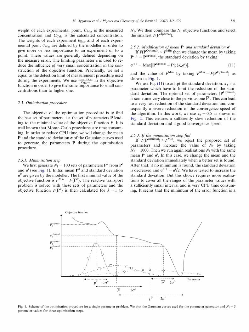
2.5.1. Minimisation step

We first generate NI = 100 sets of parameters Pk from Pi

and ri (see Fig. 1). Initial mean P0 and standard deviationr0 are given by the modeller. The first minimal value of theobjective function is F Min ¼ F ðP0Þ. The reactive transportproblem is solved with these sets of parameters and theobjective function F(Pk) is then calculated for k = 1 to

0OptimalF

02σ0P

1OptimalF

1P

2OptimalF

3OptimalF

Objective function

Fig. 1. Scheme of the optimisation procedure for a single parameter problem.parameter values for three optimisation steps.

NI. We then compare the NI objective functions and selectthe smallest F(POptimal).

2.5.2. Modification of mean Pi and standard deviation ri

If F(POptimal) < FMin then we change the mean by takingPiþ1 ¼ POptimal, the standard deviation by taking

riþ1 ¼Max½jPOptimal � Pj; ðarriÞ�; ð11Þ

and the value of FMin by taking FMin = F(POptimal) asshown in Fig. 1.

We use Eq. (11) to adapt the standard deviation. ar is aparameter which have to limit the reduction of the stan-dard deviation. The optimal set of parameters (POptimal)is sometime very close to the pervious one Pi. This can leadto a very fast reduction of the standard deviation and con-sequently a severe reduction of the convergence speed ofthe algorithm. In this work, we use ar = 0.5 as shown inFig. 2. This ensures a sufficiently slow reduction of thestandard deviation and a good convergence speed.

2.5.3. If the minimisation step fail

If F(POptimal) > FMin, we reject the proposed set ofparameters and increase the value of NI by takingNI = 1000. Then we run again realisations NI with the samemean Pi and ri. In this case, we change the mean and thestandard deviation immediately when a better set is found.After that, if no minimum is found, the standard deviationis decreased and ri+1 = ri/2. We have tested to increase thestandard deviation. But this choice requires more realisa-tions to cover all the ranges of the parameter values witha sufficiently small interval and is very CPU time consum-ing. It seems that the minimum of the error function is a

12σ

2P

22σ

3P

32σParameter

We plot the Gaussian curves used for the parameter generator and NI = 5

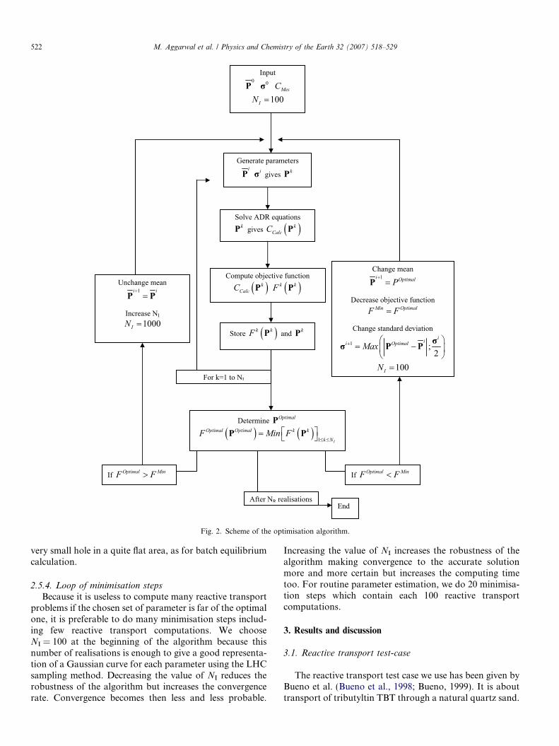
Fig. 2. Scheme of the optimisation algorithm.


very small hole in a quite flat area, as for batch equilibriumcalculation.

2.5.4. Loop of minimisation stepsBecause it is useless to compute many reactive transport

problems if the chosen set of parameter is far of the optimalone, it is preferable to do many minimisation steps includ-ing few reactive transport computations. We chooseNI = 100 at the beginning of the algorithm because thisnumber of realisations is enough to give a good representa-tion of a Gaussian curve for each parameter using the LHCsampling method. Decreasing the value of NI reduces therobustness of the algorithm but increases the convergencerate. Convergence becomes then less and less probable.

Increasing the value of NI increases the robustness of thealgorithm making convergence to the accurate solutionmore and more certain but increases the computing timetoo. For routine parameter estimation, we do 20 minimisa-tion steps which contain each 100 reactive transportcomputations.

3. Results and discussion

3.1. Reactive transport test-case

The reactive transport test case we use has been given byBueno et al. (Bueno et al., 1998; Bueno, 1999). It is abouttransport of tributyltin TBT through a natural quartz sand.


In their work, Bueno et al. (1998) provide breakthroughcurves of TBT at seven different pH. This lead to sevendifferent sets of Langmuir parameters. From Langmuirparameters obtained by these authors at pH = 6.1, equilib-rium constants and site concentration for the sorption ofTBT onto the natural quartz sand can be calculated. Thisis done in Bueno (1999) under the assumption of a DLMsurface complexation. Specific area of this sand is given byBueno et al. (1998). All these parameters and the chemicalreactions assumed in the system are summarised in Table1. The experimental column is 20 cm long, discretized in20 cells.

In the case of the sorption of TBT on a natural quartzsand, acidity equilibrium constants of BS–OHþ2 and „S–O� (Table 1) are correlated through the PZC (point zerocharge) of the sand which is PZC ’ 6 (Bueno, 1999)

PZC ¼ 1

2logðKBS–OHþ

2Þ � logðKBS–O�Þ

h i¼ 6� 1: ð12Þ

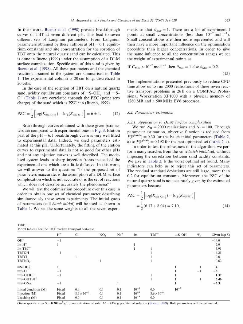
Breakthrough curves obtained with these given parame-ters are compared with experimental ones in Fig. 3. Elutionpart of the pH = 6.1 breakthrough curve is very well fittedto experimental data. Indeed, we used parameters esti-mated at this pH. Unfortunately, the fitting of the elutioncurves to experimental data is not so good for other pHsand not any injection curves is well described. The mode-lised system leads to sharp injection fronts instead of theexperimental one which are a little diffusive. In this work,we will answer to the question: ‘‘Is the proposed set ofparameters inaccurate, is the assumption of a DLM surfacecomplexation which is not accurate or is the set of reactionswhich does not describe accurately the phenomena?’’

We will test the optimisation procedure over this case inorder to obtain one set of chemical parameter describingsimultaneously these seven experiments. The initial guessof parameters (call batch initial) will be used as shown inTable 1. We set the same weights to all the seven experi-

Table 1Morel tableau for the TBT reactive transport test-case

H+ Cl� NO�3 Na+

OH� �1Im H+ 1Im TBT+

TBTOH �1TBTCl 1TBTNO3 1

BS–OHþ2 1„S–O� �1„S–OTBT+ �1„S–OHTBT+

„S–ONa �1 1

Initial condition (M) Fixed 0.0 0.1 0.1Injection (M) Fixed 8.6 · 10�6 0.1 0.1Leaching (M) Fixed 0.0 0.1 0.1

Given specific area S = 0.200 m2 g�1, concentration of solid M = 4358 g per li

ments so that hExp = 1. There are a lot of experimentalpoints at small concentrations (less than 10�7 mol l�1).Small concentrations are then more represented and willthen have a more important influence on the optimisationprocedure than higher concentrations. In order to givethe same influence to all the concentration ranges we setthe weight of experimental points as

If CMes > 10�7 mol l�1 then hMes ¼ 1 else hMes ¼ 0:2:

ð13Þ

The implementations presented previously to reduce CPUtime allow us to run 2000 realisations of these seven reac-tive transport problems in 26 h on a COMPAQ Profes-sional Workstation XP1000 with a physical memory of1280 MB and a 500 MHz EV6 processor.

3.2. Parameters estimation

3.2.1. Application to DLM surface complexation

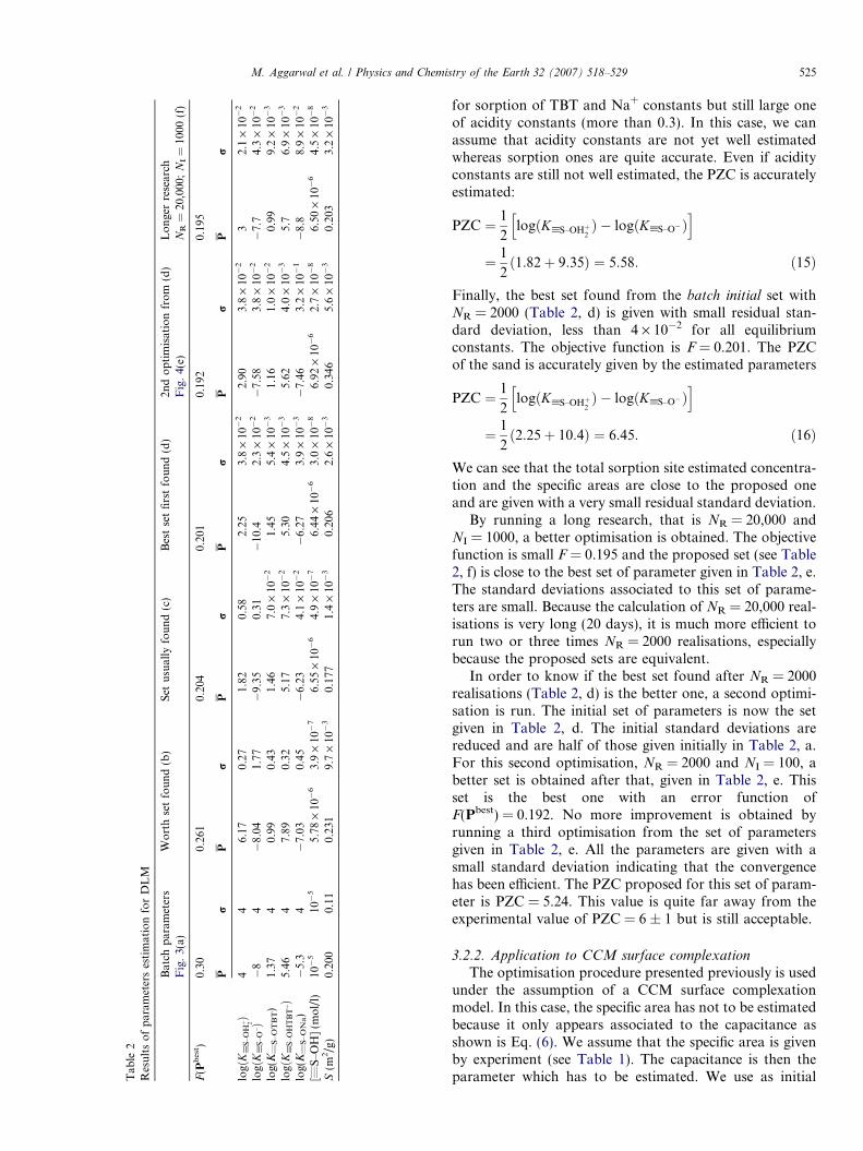
We run NR = 2000 realisations and NI = 100. Throughparameter estimation, objective function is reduced fromF(Pbatch) = 0.30 for the batch initial parameters (Table 2,a) to F(Pbest) = 0.192 for the best optimised set (Table 2, e).

In order to test the robustness of the algorithm, we per-form many searches from the same batch initial set, withoutimposing the correlation between sand acidity constants.We give in Table 2, b the worst optimal set found. Manyindicators can help us to reject this set of parameters.The residual standard deviations are still large, more than0.2 for equilibrium constants. Moreover, the PZC of thenatural quartz sand is not accurately given by the estimatedparameters because

PZC ¼ 1

2logðKBS–OHþ


h i¼ 1

2ð6:17þ 8:04Þ ¼ 7:10; ð14Þ

Im TBT+ „S–OH Ws Given log(K)

�14.01 7.01 1 3.91

1 �6.251 0.61 0.62

1 1 4

1 �1 �8

1 1 1.37

1 1 1 5.46

1 �5.3

10�3 0.0 10�5

10�3 8.6 · 10�6

10�3 0.0

ter of solution (Bueno, 1999). Bolt parameters will be estimated.

0 40 600.0

0 2

2.0x10-7

4.0x10-7

6.0x10-7

8.0x10-7

TB

T (

mol

/l)

V/Vp

Experimental Modelling

pH = 2.5

0 20 40 600.0

2.0x10-7

4.0x10-7

6.0x10-7

8.0x10-7

TB

T (

mol

/l)

V/Vp


pH = 4.1

0 20 40 60 800.0

2.0x10-7

4.0x10-7

6.0x10-7

8.0x10-7

TB

T (

mo

l/l)

V/Vp


pH = 5.2

0 20 40 60 80 1000.0

2.0x10-7

4.0x10-7

6.0x10-7

8.0x10-7

TB

T (

mol

/l)

V/Vp


pH = 6.1

0 20 40 60 80 1000.0

2.0x10-7

4.0x10-7

6.0x10-7

8.0x10-7

TB

T (

mol

/l)

V/Vp


pH = 7.1

0 20 40 60 80 1000.0

2.0x10-7

4.0x10-7

6.0x10-7

8.0x10-7

TB

T (

mol

/l)

V/Vp


pH = 7.9

0 20 40 60 800.0

2.0x10-7

4.0x10-7

6.0x10-7

8.0x10-7

TB

T (

mol

/l)

V/Vp


pH = 9.7

Fig. 3. Elution curves obtained with batch initial parameters from Bueno et al. (1998). Error function F = 0.3 and parameters values are given inTable 2, a.


instead of having PZC = 6 ± 1 (12) from experimentaldata.

On the other hand, another set found (Table 2, c) isgiven with small residual standard deviation, less than 0.1

Tab

le2

Res

ult

so

fp

aram

eter

ses

tim

atio

nfo

rD

LM

Bat

chp

aram

eter

sF

ig.

3(a)

Wo

rth

set

fou

nd

(b)

Set

usu

ally

fou

nd

(c)

Bes

tse

tfi

rst

fou

nd

(d)

2nd

op

tim

isat

ion

fro

m(d

)F

ig.

4(e)

Lo

nge

rre

sear

chN

R=

20,0

00;

NI

=10

00(f

)

F(P

bes

t )0.

300.

261

0.20

40.

201

0.19

20.

195

Pr

Pr

Pr

Pr

Pr

Pr

logð

KB

S–O

Hþ 2Þ

44

6.17

0.27

1.82

0.58

2.25

3.8

·10�

22.

903.

8·

10�

23

2.1

·10�

2

logð

KB

S–O� Þ

�8

4�

8.04

1.77

�9.

350.

31�

10.4

2.3

·10�

2�

7.58

3.8

·10�

2�

7.7

4.3

·10�

2

log(

K„

S–O

TB

T)

1.37

40.

990.

431.

467.

0·

10�

21.

455.

4·

10�

31.

161.

0·

10�

20.

999.

2·

10�

3

logð

KB

S–O

HT

BTþ Þ

5.46

47.

890.

325.

177.

3·

10�

25.

304.

5·

10�

35.

624.

0·

10�

35.

76.

9·

10�

3

log(

K„

S–O

Na)

�5.

34

�7.

030.

45�

6.23

4.1

·10�

2�

6.27

3.9

·10�

3�

7.46

3.2

·10�

1�

8.8

8.9

·10�

2

[„S

–OH

](m

ol/

l)10�

510�

55.

78·

10�

63.

9·

10�

76.

55·

10�

64.

9·

10�

76.

44·

10�

63.

0·

10�

86.

92·

10�

62.

7·

10�

86.

50·

10�

64.

5·

10�

8

S(m

2/g

)0.

200

0.11

0.23

19.

7·

10�

30.

177

1.4

·10�

30.

206

2.6

·10�

30.

346

5.6

·10�

30.

203

3.2

·10�

3


for sorption of TBT and Na+ constants but still large oneof acidity constants (more than 0.3). In this case, we canassume that acidity constants are not yet well estimatedwhereas sorption ones are quite accurate. Even if acidityconstants are still not well estimated, the PZC is accuratelyestimated:

PZC ¼ 1

2logðKBS–OHþ


h i¼ 1

2ð1:82þ 9:35Þ ¼ 5:58: ð15Þ

Finally, the best set found from the batch initial set withNR = 2000 (Table 2, d) is given with small residual stan-dard deviation, less than 4 · 10�2 for all equilibriumconstants. The objective function is F = 0.201. The PZCof the sand is accurately given by the estimated parameters

PZC ¼ 1

2logðKBS–OHþ


h i¼ 1

2ð2:25þ 10:4Þ ¼ 6:45: ð16Þ

We can see that the total sorption site estimated concentra-tion and the specific areas are close to the proposed oneand are given with a very small residual standard deviation.

By running a long research, that is NR = 20,000 andNI = 1000, a better optimisation is obtained. The objectivefunction is small F = 0.195 and the proposed set (see Table2, f) is close to the best set of parameter given in Table 2, e.The standard deviations associated to this set of parame-ters are small. Because the calculation of NR = 20,000 real-isations is very long (20 days), it is much more efficient torun two or three times NR = 2000 realisations, especiallybecause the proposed sets are equivalent.

In order to know if the best set found after NR = 2000realisations (Table 2, d) is the better one, a second optimi-sation is run. The initial set of parameters is now the setgiven in Table 2, d. The initial standard deviations arereduced and are half of those given initially in Table 2, a.For this second optimisation, NR = 2000 and NI = 100, abetter set is obtained after that, given in Table 2, e. Thisset is the best one with an error function ofF(Pbest) = 0.192. No more improvement is obtained byrunning a third optimisation from the set of parametersgiven in Table 2, e. All the parameters are given with asmall standard deviation indicating that the convergencehas been efficient. The PZC proposed for this set of param-eter is PZC = 5.24. This value is quite far away from theexperimental value of PZC = 6 ± 1 but is still acceptable.

3.2.2. Application to CCM surface complexation

The optimisation procedure presented previously is usedunder the assumption of a CCM surface complexationmodel. In this case, the specific area has not to be estimatedbecause it only appears associated to the capacitance asshown is Eq. (6). We assume that the specific area is givenby experiment (see Table 1). The capacitance is then theparameter which has to be estimated. We use as initial

Tab

le3

Co

mp

aris

on

of

surf

ace

com

ple

xati

on

mo

del

s

DL

M(a

)C

CM

(b)

TL

Mo

ut–

ou

t(c

)T

LM

in–i

n(d

)T

LM

in–o

ut

(e)

TL

Mo

ut–

in(f

)

F(P

bes

t )0.

192

0.19

20.

193

0.20

80.

189

0.19

1

Pr

Pr

Pr

Pr

Pr

Pr

logð

KB

S–O

Hþ 2Þ

2.90

3.8

·10�

22.

872.

6·

10�

22.

874.

2·

10�

42.

841.

6·

10�

32.

788.

8·

10�

32.

811.

2·

10�

1

logð

KB

S–O� Þ

�7.

583.

8·

10�

2�

8.11

4.4

·10�

2�

7.53

4.8

·10�

�7.

593.

5·

10�

3�

7.78

3.5

·10�

3�

7.56

1.2

·10�

1

log(

K„

S�

OT

BT

)1.

161.

0·

10�

21.

043.

7·

10�

21.

10o

ut

7.9

·10�

51.

09in

4.4

·10�

41.

11in

6.5

·10�

41.

10o

ut

1.2

·10�

1

logð

KB

S–O

HT

BTþ Þ

5.62

4.0

·10�

35.

622.

3·

10�

25.

60o

ut

3.9

·10�

45.

58in

2.1

·10�

35.

60o

ut

5.5

·10�

45.

66in

1.2

·10�

1

log(

K„

S�

ON

a)

�7.

463.

2·

10�

1�

6.85

1.4

·10�

2�

10.1

3.7

·10�

2�

7.49

7.5

·10�

3�

8.96

2.2

·10�

2�

7.14

1.2

·10�

1

[„S

–OH

](m

ol/

l)6.

92·

10�

62.

7·

10�

86.

76·

10�

63.

7·

10�

97.

17·

10�

67.

2·

10�

11

7.19

·10�

61.

4·

10�

10

7.17

·10�

63.

4·

10�

96.

55·

10�

61.

6·

10�

8

S(m

2/g

)0.

346

5.6

·10�

30

.20

0.19

93.

5·

10�

30.

231

7.0

·10�

50.

231

2.4

·10�

50.

196

3.7

·10�

4

cap

/cap

inn

er(F

m)�

21.

309.

6·

10�

53.

731.

3·

10�

23.

506.

6·

10�

24.

085.

7·

10�

25.

532.

5·

10�

1

cap

Ou

ter

(Fm�

2)

0.46

27.

7·

10�

30.

265

3.2

·10�

20.

265

1.4

·10�

20.

399

2.5

·10�

1

Sp

ecifi

car

eaS

for

CC

Msu

rfac

eco

mp

lexa

tio

n(b

olt

)is

give

nb

yex

per

imen

tal

mea

sure

men

t(B

uen

o,

1999

)an

dis

no

tes

tim

ated

.


value for this parameter a medium value found in the liter-ature (Lutzenkirchen, 1999) for other oxides, TiO2 andRuO2. We take cap = 1.2 ± 0.1. After running 10 cyclesof 20 minimisation loops (100 reactive transport computa-tion), we select the better set of parameters. This set is usedas initial guess for a new cycle of 20 minimisation loops.Through this way, it is possible to determine if the pro-posed set is a real minimum or not. In the case of theCCM parameter estimation, we get a definitive minimumat the third stage of the procedure.

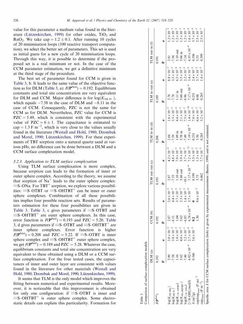
The best set of parameter found for CCM is given inTable 3, b. It leads to the same value of the objective func-tion as for DLM (Table 3, a): F(Pbest) = 0.192. Equilibriumconstants and total site concentration are very equivalentfor DLM and CCM. Major difference is for logðKBS–O�Þ,which equals �7.58 in the case of DLM and �8.11 in thecase of CCM. Consequently, PZC is not the same forCCM as for DLM. Nevertheless, PZC value for CCM isPZC = 5.49, which is consistent with the experimentalvalue of PZC = 6 ± 1. The capacitance is estimated tocap = 1.3 F m�2, which is very close to the values usuallyfound in the literature (Westall and Hohl, 1980; Dzombakand Morel, 1990; Lutzenkirchen, 1999). For these experi-ments of TBT sorption onto a natural quartz sand at var-ious pHs, no difference can be done between a DLM and aCCM surface complexation model.

3.2.3. Application to TLM surface complexation

Using TLM surface complexation is more complex,because sorption can leads to the formation of inner orouter sphere complex. According to the theory, we assumethat sorption of Na+ leads to the outer sphere complex:„S–ONa. For TBT+ sorption, we explore various possibil-ities: „S–OTBT or „S–OHTBT+ can be inner or outersphere complexes. Combination of all these possibili-ties implies four possible reaction sets. Results of parame-ters estimation for these four possibilities are given inTable 3. Table 3, c gives parameters if „S–OTBT and„S–OHTBT+ are outer sphere complexes. In this case,error function is F(Pbest) = 0.193 and PZC = 5.20. Table3, d gives parameters if „S–OTBT and „S–OHTBT+ areinner sphere complexes. Error function is higherF(Pbest) = 0.208 and PZC = 5.22. If „S–OTBT is innersphere complex and „S–OHTBT+ outer sphere complex,we get F(Pbest) = 0.189 and PZC = 5.28. Whatever the case,equilibrium constants and total site concentration are veryequivalent to these obtained using a DLM or a CCM sur-face complexation. For the four tested cases, the capaci-tances of inner and outer layer are consistent with valuesfound in the literature for other materials (Westall andHohl, 1980; Dzombak and Morel, 1990; Lutzenkirchen, 1999).

It seems that TLM is the only model which improves thefitting between numerical and experimental results. More-over, it is noticeable that this improvement is obtainedfor only one configuration: if „S–OTBT is inner and„S–OHTBT+ is outer sphere complex. Some electro-static details can explain this particularity. Formation for


„S–OTBT needs the interaction between a negativelycharged species, „S–O� and a positively charged one,TBT+. This interaction authorises a contact between thetwo reactants and allows then the existence of an innersphere complex. On the other hand, the formation of„S–OHTBT+ involves the interaction between a positivelycharged species TBT+ and neutral one „S–OH. Moreover,the electro negativity difference between O and H impliesthat O is negative and H positive. One can write: „S–Od–H+d. The electrical potential of the inner layer is thennecessary to explain the stability of „S–OHTBT+: TBT+

is located in the outer layer and is attached to „S–Od–H+d through the potential of the inner layer, if it is nega-tive. Without any preliminary indication, results providesby our parameters estimation are consistent with the elec-trostatic interaction theory.

Nevertheless, TLM surface complexation involves theuse two additional parameters, but does not induces a sig-nificant increase of the fitting between numerical andexperimental results. It seems that all the studded surfacecomplexation models leads to equivalent results.

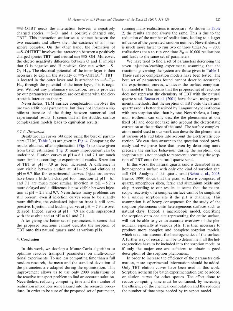
3.2.4. DiscussionBreakthrough curves obtained using the best of param-

eters (TLM, Table 3, e) are given in Fig. 4. Comparing theresults obtained after optimisation (Fig. 4) to these givenfrom batch estimation (Fig. 3) many improvement can beunderlined. Elution curves at pH = 6.1 and 7.1 are muchmore similar according to experimental results. Retentionof TBT at pH = 7.9 as been increased. A difference isnow visible between elution at pH = 2.5 and elution atpH = 9.7 like for experimental curves. Injections curveshave been a little bit changed too. Injection at pH = 6.1and 7.1 are much more similar, injection at pH = 5.2 ismore delayed and a difference is now visible between injec-tion at pH = 2.5 and 9.7. Nevertheless many problems arestill present: even if injection curves seem to be slightlymore diffusive, the calculated injection front is still com-pressive. Injection and leaching curves at pH = 7.9 are overdelayed. Indeed, curves at pH = 7.9 are quite superposedwith these obtained at pH = 6.1 and 7.1.

After giving the better set of parameters, it seems thatthe proposed reactions cannot describe the sorption ofTBT onto this natural quartz sand at various pHs.

4. Conclusion

In this work, we develop a Monte-Carlo algorithm tooptimise reactive transport parameters on multi-condi-tional experiments. To use less computing time than a fullrandom research, the mean and the standard deviation ofthe parameters are adapted during the optimisation. Thisimprovement allows us to use only 2000 realisations ofthe reactive transport problem to find an accurate solution.Nevertheless, reducing computing time and the number ofrealisation introduces some hazard into the research proce-dure. In order to be sure of the proposed set of parameter,

running many realisations is necessary. As shown in Table2, the results are not always the same. This is due to thereduction of the number of realisations, leading to a largerinfluence of the generated random number. Nevertheless, itis much more faster to run two or three times NR = 2000realisations than to run one time NR = 10,000 realisationsand leads to the same set of parameters.

We have tried to find a set of parameters describing theseven injection-leaching experiments assuming that thereactions governing the system are those given in Table 1.Three surface complexation models have been tested. Thebest set of parameters found cannot describe accuratelythe experimental curves, whatever the surface complexa-tion model is. This means that the proposed set of reactionsdoes not represent the chemistry of TBT with the naturalquartz sand. Bueno et al. (2001) have shown, using exper-imental methods, that the sorption of TBT onto the naturalquartz sand is better described by Langmuir-type isothermswith two sorption sites than by one. Nevertheless, a Lang-muir isotherm can only describe the phenomena at onefixed pH and does not take into account the electrostaticcorrection at the surface of the sand. The surface complex-ation model used in our work can describe the phenomenaat various pHs and takes into account the electrostatic cor-rection. We can then answer to the question posed previ-ously and we prove here that, even by describing moreprecisely the surface behaviour during the sorption, onesorption site is not enough to represent accurately the sorp-tion of TBT onto the natural quartz sand.

In this work, the natural quartz sand is described as anhomogeneous surface with only one kind of sorption site:„S–OH. Analysis of this quartz sand (Behra et al., 2003;Bueno, 1999) shows that the grain surface is composed ofquartz, amorphous silica, ferric and aluminium oxide andclay. According to our results, it seems that the macro-scopic reactivity of a complex surface cannot be simplifiedto a unique sorption site if the pH is changing. Thisassumption is of heavy consequence for the study of thesorption phenomena onto heterogeneous surfaces such asnatural clays. Indeed, a macroscopic model, describingthe sorption onto one site representing the entire surface,will not be able to give an accurate overview of the phe-nomena, especially at various pHs. It is then necessary toproduce more complex and complete sorption models,which take into account the heterogeneities of the surface.A further way of research will be to determine if all the het-erogeneities have to be included into the sorption model orif only the major one are sufficient to obtain a gooddescription of the sorption phenomena.

In order to increase the efficiency of the parameter esti-mation, more experimental information should be added.Only TBT elution curves have been used in this work.Sorption isotherm for batch experimentation can be added,or elution curves for other species. The effort done toreduce computing time must be continued, by increasingthe efficiency of the chemical computation and the reducingthe number of time steps needed by transport model.

0 20 40 600.0

2.0x10-7

4.0x10-7

6.0x10-7

8.0x10-7

TB

T(m

ol/l)

V/Vp


pH= 2.5

0 20 40 600.0

2.0x10-7

4.0x10-7

6.0x10-7

8.0x10-7

TB

T m

ol/l)

V/Vp


pH= 4.1

0 20 40 60 800.0

2.0x10-7

4.0x10-7

6.0x10-7

8.0x10-7

TB

T(m

ol/l)

V/Vp


pH= 5.2

0 20 40 60 80 1000.0

2.0x10-7

4.0x10-7

6.0x10-7

8.0x10-7

TB

T(m

ol/l)

V/Vp

ExperimentalModelling

pH= 6.1

0 20 40 60 80 1000.0

2.0x10-7

4.0x10-7

6.0x10-7

8.0x10-7

TB

T(m

ol/l)

V/Vp


pH= 7.1

0 20 40 60 80 1000.0

2.0x10-7

4.0x10-7

6.0x10-7

8.0x10-7

TB

T(m

ol/l)

V/Vp


pH=7.9

0 20 40 600.0

2.0x10-7

4.0x10-7

6.0x10-7

8.0x10-7

TB

T(m

ol/l)

V/Vp


pH= 9.7

Fig. 4. Elution curves after optimisation with our algorithm. Estimated parameters obtained for a Triple Layer Model where „S–OTBT is inner spherecomplex and „S–OHTBT+ is outer sphere complex. F = 0.189 and P are given in Table 3, e.


The algorithm presented here is a useful tool to validateor invalidate different sorption models but it still needsvery long computing times. It must then be improved

before to be tested over the more complicated chemical sys-tem describing the sorption of radionuclides onto naturalclays.


Acknowledgements

We thank Delphine Tovo (Ecole Nationale des Ingeni-eurs en Art Chimique et Technologique de Toulouse) forpreliminary work during her engineer internship and AmiMarxer for helpful comments. We thank Maıte Buenofor providing experimental data. M. Aggarwal has beensupported by a grant from EGIDE. This work is supportedby GdR MoMaS.

References

Behra, Ph., Lecarme-Theobald, E., Bueno, M., Ehrhardt, J.J., 2003.Sorption of tributyltin onto a natural quartz sand. J. Colloid Interf.Sci. 263, 4–12.

Brassard, P., Bodurtha, P., 2000. A feasible set for chemical speciationproblems. Comput. Geosci. 26, 277–291.

Bueno, M., 1999. Etude dynamique des processus de sorption–desorptiondu tributyletain sur un milieu poreux d’origine naturelle. Ph. D. Thesis,Universite de Pau et des Pays de l’Adour.

Bueno, M., Astruc, A., Astruc, M., Behra, Ph., 1998. Dynamic sorptivebehavior of tributyltin on quartz sand at low concentration levels:effect of pH, flow rate, and monovalent cations. Environ. Sci. Technol.32, 3919–3925.

Bueno, M., Astruc, A., Lambert, J., Astruc, M., Behra, Ph., 2001. Effect ofsolid surface composition on the migration of tributyltin in ground-water. Environ. Sci. Technol. 35, 1411–1419.

Carrayrou, J., 2001. Modelisation du transport de solutes reactifs en milieuporeux sature. Ph. D. Thesis, Universite Louis Pasteur Strasbourg I.

Carrayrou, J., Mose, R., Behra, Ph., 2002. New efficient algorithm forsolving thermodynamic chemistry. AIChE J. 48, 894–904.

Carrayrou, J., Mose, R., Behra, Ph., 2003. Modelling reactive transport inporous media: iterative scheme and combination of discontinuous andmixed-hybrid finite elements. CR Acad. Sci., Ser. II Univers. 331, 211–216.

Dzombak, D.A., Morel, F.M.M., 1990. Surface Complexation Modelling:Hydrous Ferric Oxide. Wiley-Intersciences, New York.

Hardyanto, W., 2003. Groundwater modelling taking into accountprobabilistic uncertainties. 10 Freiberg on-line Geosciences.

Lutzenkirchen, J., 1999. The constant capacitance model and variableionic strength: an evaluation of possible applications and applicability.J. Colloid Interf. Sci. 217, 8–18.

Marshall, S.L., 2003. Generalized least-squares parameter estimation frommultiequation implicit models. AIChE J. 49, 2577–2594.

Sigg, L., Behra, Ph., Stumm, W., 2000. Chimie des milieux aquatiques.Dunod, Paris.

Steefel, C.I., McQuarrie, K.T.B., 1996. Approaches to modelling ofreactive transport in porous media. In: Lichtner, P.C., Steefel, C.I.,Oelkers, E.H. (Eds.), Reactive Transport in Porous Media. Mineral-ogical Society of America, Washington, pp. 82–129.

Stumm, W., 1992. Chemistry of the Solid–water Interface. Wiley-Interscience, New York.

Vikhansky, A., Kraft, M., 2004. A Monte Carlo methods for identificationand sensitivity analysis of coagulation processes. J. Comput. Phys. 200,50–59.

Westall, J.C., 1982. FITEQL ver. 2.1. Department of Chemistry, OregonState University, Corvallis.

Westall, J.C., Hohl, H., 1980. A comparison of electrostatic models for theoxide/solution interface. Adv. Colloid Interf. Sci. 12, 265–294.

Yeh, G.T., Tripathi, V.S., 1989. A critical evaluation of recent develop-ments in hydrogeochemical transport models of reactive multichemicalcomponents. Water Resour. Res. 25, 93–108.

Zhang, T., Guay, M., 2002. Adaptive parameter estimation for microbialgrowth kinetics. AIChE J. 48, 607–616.

Documents

Parameters estimation for reactive transport: A way to test the validity of a reactive model