1

Parametric Critical Path Analysis for EventNetworks with Minimal and Maximal Time Lags

Joost van Pinxten∗, Marc Geilen∗, Martijn Hendriks‡, Twan Basten∗‡∗Department of Electrical Engineering, Eindhoven University of Technology, Eindhoven, The Netherlands‡Embedded Systems Innovation, Netherlands Organisation for Applied Scientific Research, Eindhoven, The

Netherlands

Abstract—High-end manufacturing systems are cyber-physicalsystems where productivity depends on the close cooperation ofmechanical (physical) and scheduling (cyber) aspects. Mechanicaland control constraints impose minimal and maximal time dif-ferences between events in the product flow. Sequence-dependentconstraints are used by a scheduler to optimize system produc-tivity while satisfying operational requirements. The numerousconstraints in a schedule are typically related to a relatively smallset of parameters, such as speeds, lengths, or settling times. Wecontribute a parametric critical path algorithm that identifiesbottlenecks in terms of the feasible parameter combinations. Thisalgorithm allows analysis of schedules to identify bottlenecks interms of the underlying cause of constraints. We also contributea way to find Pareto-optimal cost-performance trade-offs andtheir associated parameter combinations. These results are usedto quantify the impact of relaxing constraints that hinder systemproductivity.

I. INTRODUCTION

High-end manufacturing systems are cyber-physical systems(CPSs) composed of several cooperating machines, whichhave strict timing requirements between their operations.These requirements can be modelled as minimal and maximaltiming constraints between events. Such constraints oftenoccur due to some physical or computational process, andinfluence the productivity of the system. Groups of constraintstypically share an underlying cause, such as a motor thatactuates multiple components simultaneously. The interrela-tionship of the parameters influencing the constraints areexplored during the design phase and one or several trade-offs are selected. It is of interest to quantify the relationshipof (component) parameters to the system performance.

Scheduling activities according to a set of constraints iscommon in engineering [1], research and design [2] projects,and project management [3]. Identifying and alleviating per-formance bottlenecks is a core activity for improving theperformance of schedules. The identified bottlenecks, whichare critical paths in the event network, are important hintsfor reducing the earliest completion time of the schedules.We show that such bottleneck analysis techniques can also beextended to manufacturing CPSs.

This article was presented in the International Conference on Hard-ware/Software Codesign and System Synthesis 2018 and appears as part ofthe ESWEEK-TCAD special issue. This is the Author-version of the acceptedpaper. DOI: 10.1109/TCAD.2018.2857360

c©2018 IEEE. Personal use of this material is permitted. Permission fromIEEE must be obtained for all other uses, in any current or future media,including reprinting/republishing this material for advertising or promotionalpurposes, creating new collective works, for resale or redistribution to serversor lists, or reuse of any copyrighted component of this work in other works.

In this paper, we show that it is possible and useful toextend the critical path analysis [3] technique with parametricanalysis, so that the interdependence between parameters istaken into account. In parametric analysis, the problem isto find solutions, e.g. critical paths, for all possible valuesof the parameters. Our approach first finds constraints thatcharacterize all feasible combinations of parameters and then,for all feasible combinations of parameters, a symbolic criticalpath in the form of an expression in terms of the parameters ofthe event network. We show the effectiveness of our approachand observe that the scalability is primarily determined bythe time to find the extremes of a polyhedron. Our methodprovides system designers with a quantitative approach toevaluate interaction between design parameters. We also showa method to efficiently determine the parameter combinationsthat yield Pareto-optimal performance-cost trade-offs. Systemdesigners can then take informed decisions selecting trade-offsbetween parameters.

Section II positions our work in the body of existingwork. Section III introduces terminology and notation of eventnetworks. Section IV first shows how to find critical pathsand extends the terminology with parameters that can describephysical relations; it then shows how to find expressions forcritical paths in parametrized event networks. In Section Vwe show the applicability of the method on two differentmanufacturing systems: the Twilight system [4], and a LargeScale Printer [5], [6]. These two examples show that we canquantitatively relate relaxation of parameters to productivitygains of the machine. Section VI concludes the paper.

II. RELATED WORK

Event and activity networks have been used in projectmodelling and other kinds of scheduling problems to modelminimal and maximal time lags between events or activities.We use the project modelling approach started by Roy [7],and Kerbosch and Schell [8], and further developed by El-maghraby [9]. The time lags make it possible to describeconstraints on the feasible time ranges between events in aCPS. In this paper, we use minimal and maximal time lags toexpress constraints between events in terms of parameters.

The Critical Path Method (CPM) [3] and generalizedprecedence relations (GPRs) [9] are used to model eventnetworks, and also to find critical paths in such networks.The CPM and GPRs use the difference between the occur-rence of an event in an as-soon-as-possible (ASAP) and as-late-as-possible (ALAP) schedule to determine the slack of

2

events/activities. Those with zero slack are critical, and anydelay in any of these critical events leads to an according delayin the completion of the network. It does not, however, givethe designer any insight into how much system productivityis gained when critical constraints are relaxed.

Some critical path methods assume stochastic time lags andare applied to observations of systems, such as the shiftingbottleneck detection [10]. In this method, the machines that aremost often active are regarded as the bottleneck. This methodgives an indication of the bottlenecks over time. However,this approach does not show the impact of deadlines, asimposed by maximal time lags, and can therefore hide thetrue interaction of different machines, especially when deeppipelining behaviour occurs. Stochastic time lags have alsoled to investigations of the stochastic criticality index, suchas shown in [11]. In this paper, we assume that time lags aredeterministic, and focus on the interaction between parameters.

As described in [12], when cost slopes are known forshortening activities (also known as crashing), CPM can beused with Linear Programming to give the efficient trade-offsbetween project duration and project (direct) cost. There areseveral methods available that can be applied to networks thatdo not have maximal time lags (Fondahl’s method, Siemensmethod) [12]. The work of [9] generalizes these crashingmethods such that maximal time lags can be taken intoaccount. These works, however, do not take into account thatthe underlying cause for each constraint can be shared. Thatis, each constraint is independently relaxed, and it is assumedthat other relationships remain the same. Ignoring interde-pendencies between parameters in CPSs leads to incorrectconclusions from a system perspective.

Approaches using parametric analysis for single or multipleparameters have been developed for many kinds of problems.The modified Bellman-Ford-Moore (BFM) algorithm of [13]efficiently finds all critical paths for the feasible values of asingle parameter when edge weights are integer. Our approachallows an arbitrary number of parameters, with rational num-bers as values and weights. Graphs with rational values can beused in the approach of [13] after multiplying all expressionswith an integer factor such that all rational numbers becomeinteger values.

Most methods for multiple parameters are based on theobservation that parameter combinations occur in convexregions [14], [15], [16]. Parametric analysis of synchronousdata-flow graphs has been used to determine, for example, theparameter combinations for which the same maximum cyclemean expression holds [16], [17]. The divide-and-conquerapproach from [16] shows that performance expressions can befound even when the parameters do not necessarily take integervalues. In this paper we prove that this parametric analysis canbe applied to event networks with maximal time lags.

Some work has been carried out to identify for whichparameter combinations parametrized models have feasiblesolutions. The work of Elmaghraby [9] introduces flexibilityof an activity/constraint in an activity network as the amountof time it can be increased/decreased such that all constraintscan still be met in a schedule; i.e. it indicates when networksbecome infeasible. The convexity of parameter regions has

also been used by [18] to determine for which parametercombinations a periodic fixed priority system is schedulable.The interaction between tasks and their relation to systemutilization are modelled with fixed priority scheduling rules,and precedence relations between tasks are explicitly notallowed in their work.

Several parametric methods have also been developed fortimed automata [15], [19]. In [15] a subclass of parametrictimed automata has been identified for which it can decide onthe emptiness problem when automaton variables are upperand lower bounded by parameters. A parameter may eitheroccur in some lower bounds, or in some upper bounds, butnever in both. The approach of [15] can detect parametercombinations for which the system does not have conflictingrequirements, i.e., is feasible. Our extension of the parametricmethod allows parameters both in lower and upper bounds(minimum and maximum time lags). In [19], the feasibility ofactivating a set of real time tasks is checked through parametrictimed automata. Similar to the work of [18] the approachdoes not allow precedence constraints, as it models interactionbetween tasks through periodic activation patterns.

We extend this existing body of work by finding all feasi-ble parameter combinations and their associated performancecharacterization through parametric temporal analysis of eventnetworks with minimal and maximal time lags. The quantita-tive analysis allows finding the Pareto-optimal performance-cost trade-offs.

III. EVENT NETWORKS

We adopt the following notation from the work of El-maghraby and Kamburowski [9]: an event is identified byk ∈ E = {0, . . . , N + 1} ⊂ N, and is represented by a nodein a network graph. The source node 0 represents the startevent and the sink node N + 1 represents the finish event. Anexample network is shown in Fig. 1. The realization time ofevent k is denoted tk. The realization time of the source isfixed to 0.

A minimal time lag relation from event i to event j iscaptured in the standard form: tj ≥ ti + D(i, j). Such arelation is represented by an edge (i, j) ∈ E2 from event ito event j with weight D(i, j) ∈ R. The interpretation ofthe minimal time lag D(i, j) depends on its sign. I.e., weallow maximal time lags L(i, j) from event i to event j, bytransforming them into standard form [8]:

tj ≤ ti + L(i, j) ⇐⇒ ti ≥ tj − L(i, j)

⇐⇒ ti ≥ tj +D(j, i)

That is, a positive maximal time lag L(i, j) from i to j isequal to a negative minimal time lag D(j, i) = −L(i, j) fromj to i. Task graphs with minimal and maximal time lags mayintroduce cyclic time constraints. To ensure that all events arerelated to the source, we assume that the source has minimaltime relations with zero lag to all other events. Each event,analogously, must be related to the sink, and has a minimaltime relation with zero lag to the sink node.

A network graph is equivalent to a system of inequalities.A graph is feasible if and only if there exists a solution

3

src

A B C D

sink

1

8

1

7

3

-13

-6

Fig. 1: Example event graph with given time lags betweenevents. Positive minimal time lags are shown with black edges.Negative minimal time lags are shown in dashed red edgesand represent maximal time lags or, in other words, relativedeadlines. The gray edges have zero time lag. The only criticalpath src-ACD-sink is shown with thick edges.

to its corresponding system of inequalities. Equivalently, anetwork is infeasible if and only if it has a cycle with positivecumulative weight. The earliest feasible realization time

¯tk of

an event k is the smallest number for which the system ofinequalities is feasible.

¯tk is equal to the weight of the longest

path from the source node to node k in network G:

¯tk = max

a∈paths(0→k)

∑(i,j)∈a

D(i, j)

Definition 1 (makespan). The makespan M of a graph is theearliest possible realization time of the sink node, M =

¯tN+1.

tk is the latest possible realization time of node k. The latestpossible realization tk of event k is found by subtracting thelongest path from k to the sink from the makespan:

tk = M − maxa∈paths(k→N+1)

∑(i,j)∈a

D(i, j)

For any graph, the latest possible realization time of thesink node is equal to the makespan: tN+1 = M . The possiblerealization intervals [

¯ti, ti] of the example in Fig. 1 are shown

in Fig. 2. Notably, the realization of event B can start at earliest2 time units after A, even though the relation AB allows B tostart one time unit after A. Path AB has length 1, while pathACB has length 8 − 6 = 2, i.e. the earliest realization of Bis bounded by the maximal time difference between B and C.The makespan of the graph in Fig. 1 is 11, corresponding tothe longest path src-ACD-sink. The latest realization of B is4; the longest path from B to the sink is 7, and it can thereforeoccur in the range [2, 4] without affecting the makespan.

A relation from i to j has slack S(i, j) = tj−(¯ti+D(i, j)):

the difference between the latest realization of the targetevent j and the earliest realization of the originating eventi, taking into account the minimal time between i and j. Therelation slack determines how much a relation can be increasedwithout affecting the realization time of the sink node. In theexample network, AB has a slack of 3. The relation D(A,B)is allowed to increase by 3 time units before it starts affectingthe makespan of the network. AC has slack 0, and it cannot

TABLE I: Path lengths of the example network in Fig. 3.

Path length critical if and only if

ABCD 2q + p p ≥ q + 5 ∧ 2q ≥ p+ 5ABD 3q + 5 p ≤ q + 5 ∧ p+ q ≥ 5 ∧ 3q ≥ 2pACD 2p+ 5 2q ≤ p+ 5 ∧ 3q ≤ 2p ∧ 3p ≥ 2q + 5ACBD −p+ 2q + 10 p+ q ≤ 5 ∧ 3p ≤ 2q + 5

be increased by any amount without affecting the realizationtime of the sink node.

Definition 2 (critical relation). A relation between i and j iscritical if and only if there is no relation slack: S(i, j) = 0,or equivalently:

¯ti +D(i, j) = tj .

Definition 3 (critical path). A critical path is a simple se-quence of connected critical relations (i.e. no event is traversedmore than once), originating from the source and leading tothe sink of the network.

A longest path in a network defines the makespan of thenetwork, and as such is equal to a critical path in the network.At least one critical path exists in the network as the latestallowed realization of the sink node is equal to its earliestpossible realization. The makespan of the example network is11 time units, and the critical path in the example networkis src-ACD-sink. In this example, this is the only path whichoriginates in the source, ends in the sink, and has zero slackfor each edge in the path.

IV. PARAMETRIC CRITICAL PATH ANALYSIS

In this section, we generalize the event model such thatthe time lags can be linear functions of parameters, and thenshow how to perform critical path analysis on such models.Parameters can correspond to the speed of operations, recon-figuration times, transport times, etc. An example parametrizedevent network is shown in Fig. 3, where relations betweenevents are denoted as functions of parameters p and q, suchas D(A,C) = 2p + 5. The example in Fig. 1 is an instanceof Fig. 3 with (p, q) = (3, 1). There are four simple paths inFig. 3 from the source to the sink for non-negative values ofp and q. The path lengths are listed in Table I, where the lastcolumn indicates for which part of the parameter space thepath length is maximal. The expression in the last column isconstructed as follows. Let P = {e1, e2, e3, e4} be the pathexpressions. Then ei ∈ P is critical at point p = (p, q) if andonly if ei(p) = maxe∈P(e(p)).

A. Overview of the approach

Our approach finds the critical paths for all feasible pa-rameter combinations after it finds which combinations ofparameter values have feasible results. The results of ourapproach for the example event network are illustrated inFig. 4. Fig. 4 shows four regions in the 2-d parameter space.In one region (blue), the network is infeasible. In each ofthe three other regions, different paths in the event networkare critical. Each path, and hence each region, is associatedwith its own critical path expression. The makespan of theexample in Fig. 1 is 11 time units, which corresponds to the

4

−2 −1 0 1 2 3 4 5 6 7 8 9 10 11

Time

AB BC

AC CD

BD

CB

DA

A B C D

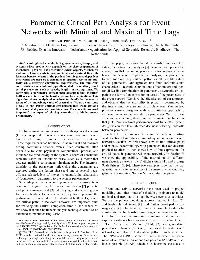
Fig. 2: Possible realization intervals for event graph shown in Fig. 1, shown in the top lane. The constraints are shown in thebottom five lanes as arrows, originating from the earliest realization time of its source event having length D(i, j). Criticaland non-critical constraints are represented with solid and dashed lines respectively.

A B C Dq

5 + p

q

5+2q

p

-13

-2p

Fig. 3: Example parametrized event network with minimal andmaximal time lags. Fig. 1 is an instance of this parametrizednetwork with (p, q) = (3, 1). The source, sink, and theirrelations have been omitted.

expression 2p+5 at (p, q) = (3, 1), which is part of the yellowregion in the figure. Parameters often relate to costs, e.g., fastertransport is more expensive. Thus the identified regions enabletrading off cost and performance. We provide further insightinto cost/performance trade-offs in Section IV-F. The rest ofthis section shows how such expressions can automatically befound for all parameter combinations in a specified range.

We start from an existing algorithm that can be appliedto non-parametrized event networks with maximal time lags(Section IV-B). As a first contribution, we use a symbolicversion of this method to find a critical path expression forone combination of the parameters (Section IV-C). We provethat such critical path expressions, as well as the conditionsfor which the network is feasible, are convex. Our secondcontribution is explained in detail in Section IV-D, where weintroduce an algorithm that removes all infeasible parametercombinations from a parameter space for a given event net-work. This algorithm provides the conditions under which fea-sible solutions exist. Our third contribution is that we introduceparametric analysis for event networks to find critical pathexpressions for each of the feasible parameter combinations(Section IV-E). We show that the divide-and-conquer methodof [16] can be extended to find all such expressions relativelyefficiently. Finally, as a fourth contribution, we show that wecan find the Pareto-optimal trade-offs for linear cost functions,and provide some interpretation of the expressions found as abasis for optimization in Section IV-F.

Infeasible 2 p+5 3 q+5 -p+2 q+10

Z

Y

X

W

V

U

T

0 1 2 3 4 5

0

1

2

3

p

q

Fig. 4: Critical path expressions and infeasible parametercombinations for the example in Fig. 3. The gray contour linesinside a polyhedron are iso-makespan lines. The extremes ofthe polyhedra are labelled with a letter.

B. Critical Path Analysis for event networks with minimal andmaximal time lags

We first show how to calculate earliest and latest realizationsfor networks with fixed minimal and maximal time lagsfor a particular parameter point. Event realization times arecalculated efficiently using a longest-path algorithm such asthe Bellman-Ford-Moore (BFM) algorithm [20], [21]. BFMhas been used in the (E)MPM algorithm [7], [8], as well asactivity networks with GPRs [9]. These algorithms also detectinfeasibility in event networks.

The BFM algorithm can provide both critical paths andinfeasible cycles. A network is infeasible when a cycle withpositive weight exists in the network. Kerbosch and Schell [8]and Sedgewick and Wayne [22] showed that it is possible tofind an arbitrary critical path by doing an ASAP analysisand keeping track of the relaxations per node. In case thenetwork is feasible, the BFM algorithm keeps track of a parent

5

tree [22] that defines which of the incoming nodes was lastused to relax a node. This data structure can be efficientlyupdated while finding the ASAP times of the events in thenetwork. A critical path can be found by following the parentrelationships from the sink node up the parent tree until thesource node has been reached. Or, in case the network isinfeasible, a positive cycle is found by tracking back the parentgraph from the sink node until a node is encountered that hasbeen visited already.

C. Parametrized event networks

In networks resulting from CPSs, the relations betweenevents are typically derived from physical or control con-straints that the CPS needs to adhere to [4], [5], [23]. It isoften possible to parametrize the relations in the event networksuch that they are linear combinations of some (physical)parameters. The travelling time t of a product at a velocityv, for example, can be modelled as the linear combination ofthe required displacement x and displacement rate δx = 1

v ,resulting in the linear relation t = x

v = x · δx. In theexample parametrized network (Fig. 3) p and q are two suchdisplacement rates, for example of two robotic arms movingat different speeds.

We first show how to assess the feasibility and the makespanof an event network for a particular parameter through thecritical path analysis detailed in Section IV-C1. We thenprove that such critical path and infeasibility expressionsrelate to geometrical half-spaces and form convex polyhedrain Section IV-C2. We use the half-space representation ina feasibility detection algorithm (Section IV-D), after whichwe apply a divide-and-conquer to find all expressions in thefeasible space (Section IV-E).

1) Relating critical paths and positive cycles to parameters:The parametric weight D(i, j)(p) of a relation r = (i, j) is aparametric affine expression e(p) = br · p+ cr, where p is avector of parameters, br is a vector of weights, cr is a constantand · denotes a vector inner product. For d parameters, theaffine function e can be represented by a vector consisting ofcoefficients br and the constant cr in the Rd+1 space, andthe function evaluation at a parameter point p ∈ Rd of ebecomes e(p) = [br cr] · [p 1]. Consequently, the makespanfor a parameter point p becomes:

M(p) = maxa∈paths(0→N+1)

∑(i,j)∈a

D(i, j)(p)

A path in the parameter space is critical if the path has

the maximal weight of all paths for some combination ofparameters. The makespan M can be expressed as a linearcombination b · p + c of the occurrences of parameters insome critical path P for all p for which the expression of Pis critical:

M(p) =∑

(i,j)∈P

D(i, j)(p) =∑

r=(i,j)∈P

br · p+ cr = b ·p+ c,

where b =∑

r∈P br and c =∑

r∈P cr.A critical path expression can only be found in case the

network has feasible solutions. Otherwise, instead of a critical

path expression, we extract a positive cycle C causing infea-sibility at a parameter point p by retrieving the expression Vof that cycle C:

V (p) =∑r∈C

br · p+ cr = b · p+ c > 0,

where b =∑

r∈C br and c =∑

r∈C cr.Any point p for which a positive cycle exists (i.e. V (p) > 0)

is infeasible. This inequality therefore defines a half-space forwhich no feasible solutions exist for the network. When thecycle BCB in Fig. 3 of length q− 2p is greater than zero, thenetwork is infeasible; we therefore recognize that all points(p, q) from the parameter space for which q − 2p > 0 areinfeasible.

2) Convex polyhedra of critical path expressions: We adaptProposition 5 from [16] to show that the critical path expres-sions form convex polyhedra in the parameter space. The proofof that proposition also applies to Proposition 1.

Proposition 1.{p ∈ Rd |M(p) = e(p)

}is a convex polyhe-

dron for any critical path expression e.

Any half-space s can be described by an affine expression esuch that s(e) = {p ∈ Rd | e(p) ≥ 0}. A convex polyhedroncan be represented as the intersection of a finite set of half-spaces, each of which is represented by an expression orvector, i.e. a polygon can be represented by a subset h ⊂ Rd+1.We lift the function s to sets of half-spaces: s(h) =

⋂e∈h s(e).

A convex polyhedron can therefore be described by a set ofexpressions that correspond to half-spaces. Proposition 2 helpsto determine the feasible parameter combinations.

Proposition 2. If all corners of a convex polyhedron with half-space representation h are feasible, then all points in s(h) arefeasible.

Proof. If there would be a parameter point p in the polyhedron(with half-space representation h) that is infeasible, then atthat point a positive cycle with cumulative weight V (x) =b ·x+c must exist such that V (p) > 0. The inequality b ·x+ccorresponds to a half-space that contains p. The half-spacecontaining p includes at least one corner point of h. Therefore,that corner point must be infeasible too. This is a contradictionand therefore proves the proposition.

D. Determining feasible parameter combinations

Consider a situation where a convex polyhedron (possiblythe entire parameter space) is explored for infeasible points,with the goal to prune these points. Algorithm 1 removesinfeasible half-spaces using the information in a positive cyclefound in the graph. If BFM (in EVALUATE) finds an infeasiblecorner point of the polyhedron, it removes the half-spacedescribed by the positive cycle expression V (p) > 0, asdefined in Section IV-C1. It does so by adding the restriction−V (p) ≥ 0 to the polyhedron. The algorithm continues in arecursive fashion with the remaining space until all cornerpoints are feasible. This process is illustrated in Fig. 5a-5d. The result is returned through the recursive calls. FromProposition 2 it follows that all parameter combinations inthat (possibly empty) polyhedron are feasible.

6

-1 1 2 3 4 5 6

-1

1

2

3

4

5

6

2 p-8 ≤ 0

(a) Alg. 1: remove infeasible re-gion (ACDA) 2p− 8 > 0

-1 1 2 3 4 5 6

-1

1

2

3

4

5

6

q-2 p ≤ 0

(b) Alg. 1: remove infeasible re-gion (BCB) q − 2p > 0

-1 1 2 3 4 5 6

-1

1

2

3

4

5

6

3 q-8 ≤ 0

(c) Alg. 1: remove infeasible re-gion (ABDA) 3q − 8 > 0

-1 1 2 3 4 5 6

-1

1

2

3

4

5

6

-p+ 2 q- 3 ≤ 0

(d) Alg. 1: remove infeasible re-gion (ACBDA) 2q − p− 3 > 0

-1 1 2 3 4 5 6

-1

1

2

3

4

5

6

2 p+5

-p+ 2 q+ 10

3 p-2 q- 5 0

(e) Alg. 2: expression −p+ 2q + 10 6=2p+5 at (3, 3/5), split by 3p−2q−5 =0

-1 1 2 3 4 5 6

-1

1

2

3

4

5

6

-p+ 2 q+ 10

3 q+5

2 p-3 q 0

(f) Alg. 2: expression −p+ 2q + 10 6=3q+5 at (16/11, 24/25), split by −p−q + 5 = 0

-1 1 2 3 4 5 6

-1

1

2

3

4

5

6

2 p+5

3 q+5

2 p-3 q 0

(g) Alg. 2: expression 2p+ 5 6= 3q + 5at (36/10, 2), split by 2p− 3q = 0

Fig. 5: Illustration of our method for the example in Figure 3. p and q both range from 0 to 5.

Algorithm 1 Determine feasible parameter combinations

1: function DETERMINEFEASIBLEPOINTS(event networkG, convex polyhedron CP )

2: for each corner ci of s(CP ) do3: feasible, cycle expression = EVALUATE(G, ci)4: if ¬ feasible then5: CP ′ = CP ∪ {−cycle expression}6: return DETERMINEFEASIBLEPOINTS(G, CP ′)7: return CP // All points in CP are feasible

E. Divide-and-conquer

The polyhedron obtained from Algorithm 1 contains onlyfeasible points, and allows the use of the divide-and-conquerapproach presented in [16] (Algorithm 2). That approach findsall critical path expressions for all parameter combinationsby partitioning the parameter space into smaller and smallerpieces until an expression is found that holds for all cornerpoints of the polyhedron. When an expression ei found in theinterior of a polyhedron does not hold for one of its cornerpoints c with expression ec, the polyhedron is split acrossthe hyperplane ei = ec; i.e., to one polyhedron the equationei − ec ≥ 0 is added and to the other ei − ec ≤ 0. Forthe example in Fig. 3, the algorithm starts from the feasibleparameter combinations found in Fig. 5d. It finds expressionM(p, q) = 2p + 5 for the point (p, q) = (3, 3/5), whichdoes not hold at corner (0, 0) as M(0, 0) = 10 (Fig. 5e).

The expression M(p, q) = −p + 2q + 10 is found at (0, 0),and we therefore split the polyhedron into two pieces, by theequation −p+ 2q+ 10 = 2p+ 5. This process is repeated twomore times as illustrated in Fig. 5f and 5g.

Once an expression is found that holds for all corner pointsof a polyhedron, the algorithm stops exploring that part ofthe parameter space and continues with another polyhedron.For the two polyhedra found in Fig. 5f the algorithm findstwo expressions that hold in these polyhedra respectively. Itcontinues with a polyhedron for which no expression has beenfound yet in 5g. The results of Algorithm 1 and 2 are combinedin Fig. 4.

The divide-and-conquer approach of [16] is reproduced inAlgorithm 2. This algorithm requires a feasible solution to befound for an arbitrary point inside the polyhedron, along withan expression that holds for that point.

Unfortunately, no efficient algorithm is possible for gener-ating the extreme points (i.e. the corners) of a convex poly-hedron [24]. When all parameter combinations are feasible,Algorithm 2 initially needs to transform a non-degenerate setof half-spaces in d dimensions into 2d corner points. Enumer-ating an exponential number of corner points is expensive,but it turns out to be feasible for a moderate number ofparameters (e.g. ¡ 15). Furthermore, the number of calls toDIVIDECONQUER is at least the number of expressions tobe identified, and possibly more. The polyhedron for 3q + 5for the example of Fig. 3 is found by combining the resultsof two different sub-problems (Fig. 5f, 5g). Each call to

7

Algorithm 2 Divide-and-conquer

1: function DIVIDECONQUER(event network G, convexpolyhedron CP )

2: p = random point in s(CP )3: ec =FIND EXPRESSION(G, p)4: for each corner ci of s(CP ) do5: ei = FIND EXPRESSION(G, ci)6: if ec(ci) 6= ei(ci) then7: // Divide CP into two disjoint polyhedra8: CP1 = CP ∪ {ei − ec}9: CP2 = CP ∪ {ec − ei}

10: S1 = DIVIDECONQUER(G,CP1)11: S2 = DIVIDECONQUER(G,CP2)12: // Return all expressions found in polyhedra13: return S1 ∪ S2

14: return {ec} // Expression holds for each corner

FIND EXPRESSION costs at most O(|E||R|) where |E| is thenumber of events (nodes), and |R| the number of relations(edges).

In comparison with the modified BFM algorithm of Levneret al. [13], we see that their approach is more efficient fora single parameter, but it cannot take into account multipleparameters simultaneously. Their modified algorithm findsthe critical paths in O(|R|2 · |E|) time when the parametercoefficient on the relations is chosen from {−1, 0, 1}. Forarbitrary integer values, the approach takes O((b · |R|)2 · |E|),where b is the largest parameter coefficient occurring onany edge. Our method solves a generalized version of theproblem of [13], where parameters can be rational numbers,and multiple parameters are taken into account. For a givennumber of parameters, the running time of our approachdepends on the number of regions to be found, the time toevaluate a particular parameter point, and the time to convertthe half-space representation into corner points. The numberof regions that will be found depends on the parameter range,which is selected by the designer.

F. Assessing the parameter regions

The results of our approach can be used to determinethe quantitative impact of decreasing/increasing parameters.The rate of change per unit of reduction is found in thegradient ∇ of the expression in the region around the currentset-point or working point. The gradient component for asingle parameter i at a point with expression e is equal tothe aggregate contribution bi of parameter i to the criticalpath, i.e., ∇ie = bi. In Fig. 4, ∇M(3, 1) = (2, 0) and∇M(1, 1) = (−1, 2). Changing the parameter by ∆i willimpact the makespan by bi · ∆i, as long as the critical pathexpression still holds for the new parameter point, i.e., it liesin the same region.

We assume that the makespan and a cost function, sayC(p, q) = p − 2q in the example of Fig 4, are both tobe minimized. Typically, the optimal cost is found at adifferent parameter combination than the optimal makespan,and therefore trade-offs exist between makespan and cost. For

2 p + 5

3 q + 5

Z

Y,X

W

V

U

T

8 9 10 11 12 13Makespan

-2

2

4

cost

Fig. 6: Cost-makespan trade-off space for c(p, q) = p−2q forFig. 3. The labelled extremes correspond to those in Fig. 4.

example, starting from point X = (7/3, 8/3), any point onthe line segment XW in Fig. 4 closer to W has shortermakespan M = −p+2q+10 and higher cost C = p−2q. Onthe other hand, the cost-makespan trade-off at X is preferredover any of the cost-makespan points found on the line XU .The parameter selection can be improved by following thegradient such that the cost decreases or stays the same, and themakespan decreases, or vice versa. A parameter combinationis called dominated iff it is worse in at least one of the twoaspects and not better in the other than some other parametercombination.

In general, we want to find all Pareto-optimal cost-performance trade-offs in the parameter space. The Pareto-optimal parameter combinations are those for which no otherparameter combinations exist that dominate it. For an arbitrarylinear cost function C(x) = α · x, the cost and makespancan be computed for each point in the space. All Pareto-optimal parameter combinations can be found by projectingthe parameter-space to the cost-performance trade-off space,finding the trade-offs in that space and translating them backto the parameter combinations. Transforming a polyhedronfrom the parameter space to the cost-makespan space, whereM(x) = b · x+ c is the associated expression, is defined by:

T (x) =

[M(x)C(x)

]=

[b cα 0

] [x1

]=

[bα

]x+

[c0

]= P1x+p2

Applying the affine transformation T to all points of aconvex polyhedron in the parameter space yields a new convexpolyhedron in the cost-makespan space. It is sufficient totransform the extreme points of the polyhedron to obtain thepolyhedron in the cost-makespan space. An example of sucha projection is shown in Figure 6. The Pareto-optimal cornerpoints are efficiently identified in the cost-makespan space byapplying algorithms such as Simple Cull [25] to the finite setof corner points. Each point in a convex polyhedron that lieson a line between two adjacent Pareto-optimal corner points,is Pareto-optimal as well.

Transformation T is not necessarily bijective, i.e., multipleparameter combinations x may map to the same makespan-cost trade-off (M,C). Each Pareto-optimal point (M,C) ina convex region in the trade-off space can be translated back

8

to the parameter space through the (pseudo-)inverse of thetransformation associated with that convex region:

x = T †(M,C) = P1†([MC

]− p2

)Each Pareto-optimal point (M,C) on the Pareto-optimal linesegments maps to the space (T †(M,C)⊕K(P1))∩E whereE is the polyhedron corresponding to the transformation T ,and K(P1) is the kernel of P1. For two subspaces A and B,⊕ is their extension: A⊕B = {a+ b | a ∈ A, b ∈ B}. Eachextension of a kernel and a point in the parameter space is asubspace of the parameter space.

In the example of Fig. 6, the line segment XW of region3q + 5 has a transformation T with full rank P1, and eachpoint on the line segment therefore corresponds uniquely toa point on the line segment XW in the parameter space ofFig. 4. Similarly, the line segment VW for region 2p + 5maps uniquely to the line segment VW in the parameter space.However, all points of the 2-D polyhedron for the expression−p+2q+10 in Fig. 4 have been mapped to points on the lineV X in the trade-off space. Its corresponding P1 has less thanfull rank. The kernel of transformation P1 is the same for allof the Pareto-optimal line-segments, and these line segmentsmap to the intersection of two half-spaces. Each point in theregion −p + 2q + 10 is therefore a Pareto-optimal parametercombination: for example, the point Y in the cost-makespanspace maps to a line 2p+ q+ d = 0 such that the line passesthrough Z = T †(13,−3) = (8/5, 4/5) in the parameter space,i.e. d = −4. On this line, the combinations of p and q are suchthat the makespan remains the same, i.e. they coincide with aniso-makespan line, and also such that the cost does not change.As one point on the line has been shown to be Pareto-optimal,each point in the region that falls onto that line is also Pareto-optimal. The resulting Pareto-optimal parameter combinationsare thus the polyhedron for −p+ 2q + 10.

V. CASE STUDIES

We describe two case studies and perform parametrictemporal critical path analysis on them. We investigate therelative speeds of two robot arms for the Twilight system [4],and a specific reconfiguration aspect of the print head of alarge-scale printer (LSP) [6]. Algorithms 1 and 2 have beenimplemented in C++ and run on a 64-bit Ubuntu machine. Wehave used the C-library of the Double Description method [24]in combination with the GMP library [26].

A. Twilight System

The Twilight System [4] (see Fig. 7) is an example createdfor the study of controller synthesis and performance analysisof manufacturing systems. The manufacturing system pro-cesses balls that need to be drilled. Before drilling is allowed,the ball needs to be conditioned to the right temperature. First,a ball is picked up at the input buffer by the load robot (LR).Once it is brought to the conditioner (COND) it is processedimmediately. Once the conditioning of the ball has finished,it immediately needs to be transported by either one of therobots to the drill (DRILL), where it is drilled before the

LR

IN OUTCOND DRILL

UR

Fig. 7: Twilight manufacturing system, from [4].

conditioning of the ball expires. Finally, the drilled ball istransported to the output by the unload robot (UR). Figure 8depicts a simple schedule where the unload robot moves theproduct from COND to DRILL. Consider that the time it takesfor these robots to travel one unit of distance at movementspeeds vLR and vUR is LR = 1/vLR and UR = 1/vUR

respectively. Increasing LR and UR corresponds to reducingthe movement speeds.

The robots can travel either horizontally or vertically, butnot diagonally, and always need to move to the highestvertical position before moving horizontally. The horizontaldistance between input and conditioning is 10 units, fromconditioning to drilling and drilling to output is 5 distanceunits each. The vertical distance to the input box is 3 units,to the conditioning and drilling platforms 1 unit, and theball is allowed to be released at any height above the outputbuffer. Handing over a ball is synchronized and immediate.Conditioning takes exactly 9 time units and expires 8 timeunits after conditioning has finished. Drilling takes exactly 3time units. The processing rate of the conditioning, C, and thedrilling D are fixed to 1. UR and LR range between 0 and1.5. Even though they are fixed, C and D are still annotatedas parameters in the model to distinguish their contribution tothe critical paths.

Figure 9 shows the critical path expressions as function ofUR, LR, C, and D. For the given ranges, two positive cyclesare detected (blue region). UR and LR become too largeto meet the required maximum time between conditioningand finishing the drilling, leading to a positive cycle. Inthe other cycle, the time it takes for one robot to moveaway and the other to pick the ball from the conditioner istoo large, and the conditioning deadline is violated. Threecritical path regions denote the behaviour of the schedulefor particular combinations of the robot travelling rates. AsLR and UR tend towards zero, the movement speed of therobots becomes infinitely fast, and the makespan becomesM(0, 0) = 90C+3D+26LR+70UR = 90C+3D. This is alower bound on the performance imposed by the time neededfor the drilling and conditioning process.

In the green region, changes in UR have the highest impacton performance. The unload robot performs some movementsin parallel with the drilling process. Before the unload robotbecomes too slow to pick up the ball immediately after drillingends, there is another cycle that becomes positive. When theunload robot is faster than drilling, the drilling time is always

9

Load new product

Move above COND

Move away from COND

reset

wait CONDITION

reset

handover

wait

Move to COND

Move to DRILL

Move above DRILL

release collision area

Move to DRILL

reset

release collision area

handover

wait

DRILL

reset

handover

handoverMAX COND TIME

Fig. 8: Example life-cycles and scheduling dependencies for the Twilight System (Figure 7); the Load Robot (orange) loads aproduct and delivers it to the conditioning stage (purple). The Unload Robot (green) picks it up and needs to deliver it to theDrill (cyan) before the conditioning expires. Dotted edges are dependencies from the current product to the next product. Thetwo positive cycles are shown with green and blue highlighted edges.

Infeasible

9C+3D+314 LR+7UR

9C+30D+17 LR+169UR

90C+3D+26 LR+70UR

O

NM

L K

0.0 0.2 0.4 0.6 0.8 1.0 1.2 1.40.0

0.2

0.4

0.6

0.8

LR

UR

Fig. 9: Expressions for the Twilight system.

in the critical path, as shown by component 30D. In the yellowregion, the load robot is most often in the critical path. Eventhough the unload robot performs most actions, our resultshows that improving the load robot’s speed will give thehighest gain. The load robot’s speed is in the critical path moreoften due to the scheduled dependencies. In the red region, theconditioning process becomes the most important bottleneck,especially when LR and UR tend towards zero; the smallestpossible makespan for 10 products is M(0, 0) = 93 time units.This is significantly less than the largest discovered makespanM(1.5, 0) = 483 time units.

These results show that optimization efforts can be basedon the relative and absolute travelling rates of the system.This makes it possible to investigate the interaction of systemparameters and performance. Discussing such relations canbe valuable when deciding with different stake-holders aboutthe performance of the systems components, such as the

Fig. 10: LSP schematic overview, from [6].

robot travelling speeds, conditioning times and interdepen-dencies. Also cost-performance trade-offs are possible. Fig. 9shows the Pareto-optimal combinations for a cost functionC(LR,UR) = −LR− 3UR with a thick black line.

B. Large-Scale Printer

The paper path of a LSP [6] is defined as a path thatsheets follow in the printer. The paper path consists of severalmotors, switches, and functions that perform actions on thesheets. The sheets are guided on a metal track and their speedand acceleration are controlled by pinches. Figure 10 showsthe topology of a paper path. The sheets need to move twicethrough the image transfer station (ITS) before going to theoutput. Duplex sheets enter the duplex loop (DL), and a turntrack (TT) reverses the sheet’s direction, for printing on theopposite side. The sheets return from the duplex loop to themerge point (MP) within a pre-defined interval from their firstprint. The sheets are not allowed to overlap or collide with thesheets coming from the paper input module (PIM). When thesheet has been processed fully, it leaves the printer throughthe finisher (FIN).

The acceleration profiles of sheets are determined almostcompletely beforehand; a pre-determined buffer region used

10

TABLE II: Sheet specifications.

(a) Sheet details

L H

A: A4 210 0.25B: A3 420 0.1C: A3+ 483 0.3

(b) ITS reconfiguration times

CurrentA4 A3 A3+

A4 0.26 4.51 2.01A3 4.78 0.53 6.03

Prev

.

A3+ 2.35 6.10 0.60

to somewhat slow down the sheets. The range of this buffer isencoded as a minimum and maximum travelling time by thevertical edges in the example event network (Fig. 11). Eventhough the relation between acceleration profiles and minimumand maximum loop times is non-linear, separating these twovariables still allows them to be modelled as linear constraints.The horizontal and diagonal edges in the example encode thenon-overlapping constraints.

The sheets can have highly varying specifications, and themodules therefore may need to reconfigure themselves toanother operating point to achieve the required quality. Onesuch reconfiguration occurs at the ITS; the print head may needto be raised or lowered between sheets to achieve the properprint gap distance for image quality. The print head height H ,for example, can be modelled as a linear movement, whichcan be started after the previous sheet has been fully printed(i.e. has left the ITS). The ITS is ready for the next sheet whenit has moved for its full length L, and the print head movedand has stabilized:

tITS,cur = tITS,prev + ∆t

= tITS,prev +Lprev

vITS+|Hprev −Hcur|

vvert+ γ

= tITS,prev + αLprev + β|Hprev −Hcur|+ γ (1)

As the speeds vITS and vvert are constant, we can useparameters α = 1/vITS , β = 1/vvert. The equation thenbecomes a linear expression, as Hprev, Hcur, Lprev are allsheet-dependent and assumed constant. The constraint simpli-fies to the following expression when no head movement isneeded tITS,cur = tITS,prev+αLprev . Decreasing the value ofα means increasing the speed at the ITS. Decreasing β meansincreasing the speed of the vertical movement. Decreasing γmeans that oscillations dissipate faster, perhaps due to higherdamping in the system.

A repeated pattern of duplex sheets is fed into the printer,i.e. (ABC)60. The symbols A, B, C refer to one of the typesof sheets denoted in Table IIa and move at the ITS at vITS =800mm/s. The nominal speed of the head movement is 0.04units per second.

Let’s assume that the ITS is the bottleneck; the PIM andFIN are always ready to provide/receive a sheet. In the eventnetwork for the schedule for this print job (Fig. 11), each sheetreturns to the merge point in the interval tr ∈ (10, 15) fromthe first time at the merge point. The sequence of first printsand second prints that the scheduler has chosen leads to arequirement on the reconfiguration times between passes inthe sequence (diagonal edges).

J1O, 1

J1O, 2

J1O, 3

J1O, 4

J2O, 1

J2O, 2

J2O, 3

J2O, 4

J3O, 1

J3O, 2

J3O, 3

J3O, 4

J4O, 1

J4O, 2

J4O, 3

J4O, 4

J5O, 1

J5O, 2

J5O, 3

J5O, 4

J6O, 1

J6O, 2

J6O, 3

J6O, 4

J7O, 1

J7O, 2

J7O, 3

J7O, 4

J8O, 1

J8O, 2

J8O, 3

J8O, 4

J9O, 1

J9O, 2

J9O, 3

J9O, 4

J10O, 1

J10O, 2

J10O, 3

J10O, 4

645718

314106

13701975

2227579

10210379

2227579

387000

645718

314106

13701975

2227579

10210379

2227579

149999

387000

645718

314106

13701975

2227579

10210379

2227579

149999

387000

645718

314106

13701975

2227579

10210379

2227579

149999

387000

645718

314106

13701975

2227579

10210379

2227579

387000

645718

314106

13701975

2227579

10210379

2227579

387000

645718

314106

149999 13701975

2227579

10210379

2227579

387000

645718

314106

2227579 13701975

2227579

10210379

2227579

387000

645718

314106

2227579 13701975

2227579

10210379

2227579

387000

645718

2227579 13701975

10210379

645718

15638119

10210379

645718

15638119

10210379

645718

15638119

10210379

645718

15638119

10210379

645718

15638119

10210379

645718

15638119

10210379

645718

15638119

10210379

645718

15638119

10210379

645718

15638119

10210379

645718

15638119

10210379

Fig. 11: Example event network and critical path for a LSPflow-shop instance with 10 products. Each column describes aproduct travelling through the flow-shop, and each row showsthe operations on each product. The second and third operation(rows) are mapped onto the same machine. Sequencing edges(diagonal) ensure that at most one product occupies themachine at any time.

Infeasible

0.01134α+90. β+6. γ+26. lmin

0.013566α+185. β+13. γ+25. lmin

0.014049α+180. β+12. γ+25. lmin

0.014238α+26. lmin

0.020244α+350. β+34. γ+22. lmin

0.02247α+402. β+41. γ+21. lmin

0.022953α+400. β+40. γ+21. lmin

0.064764α+1276. β+174. γ+2. lmin

0.067473α+1320. β+180. γ+ lmin

0.069216α+1372. β+185. γ

0.089103α+1120. β+112. γ+3. lmin

0.092295α+1162. β+117. γ+2. lmin

0.092715α+1160. β+116. γ+2. lmin

0.095004α+1206. β+123. γ+ lmin

0.00 0.05 0.10 0.15 0.200.40

0.42

0.44

0.46

0.48

0.50

β

γ

Fig. 12: Example critical path expressions for an LSP.

The critical path expressions associated with different com-binations of β and γ are shown in Fig. 12. Depending on βand γ, the majority of the time in the critical path is spenton either: (α) moving the sheet under the ITS, (β) headmovements, (γ) oscillations, (lmin) travelling through the loop.As β and γ decrease, they also occur less often in the criticalpath. The performance of the system is lower bounded by theloop time lmin, which occurs 26 times in the region with thelowest makespan. The bottleneck changes from the loop timeto the head movement parameters as β and γ increase. Theexpressions show that α becomes relevant for performance,even though only β and γ are varied in the experiment.

11

Eventually, β and γ become so large that lmax is violated.For β ≥ 0.9, the iso-makespan lines are much closer

together, showing that from this point onward, the influenceof β and γ are much higher. In these parameter ranges, themakespan is more sensitive to the head movement rate β thanto the settling time γ, as can be seen from the contributionof these components in the critical path expressions. One canconclude from this analysis that it is more meaningful to spenddevelopment effort on increasing the head movement speed,rather than reducing the settling time.

C. Evaluation

We have evaluated the DETERMINEFEASIBLEPOINTS andDIVIDECONQUER algorithms on several event networks usingdifferent parameter ranges. The examples that have beenpresented so far are summarized in Table III. The illustratedexamples have been extended by including more parameters.All experiments are run on an Intel Core i7 950 at 3GHz.

The Packing instances are variations on the Twilight ex-ample which only contain minimal time lags. Each productis modelled with 30 events, and dynamic relations existbetween events of subsequent products. The time constraints ofthe relations have been determined stochastically by drawingfrom several PERT distributions, and are associated withtheir respective machines, UR or LR. The resulting networkis a rather large directed acyclic network without negativeconstraints, and as such the topological sorting as used inCPM [3] has been used in our experiment, instead of theslower, but more generic BFM.

We observe that the number of critical paths found inthe packing cases grows with O(|E|) when only the UR isparametrized, and with O(|E|2) when both the LR and URare parametrized. We conjecture that the number of criticalpaths grows in general with O(|E|d) where d is the numberof parameters.

Due to the growing number of critical paths and cornerpoints of regions for problems with multiple parameters, boththe number of splits and the number of evaluations go up. Thetime taken for each evaluated point remains roughly the samefor each network instance, and does not depend on the numberof parameters.

VI. CONCLUSIONS

We have shown that it is possible and useful to identifyquantitative relationships between system parameters and sys-tem performance when the timing constraints in schedules areannotated in linear combinations of design parameters. Ifthe parameters have non-linear relationships, the non-linearmodel can be split into several models, for which linearisedexpressions hold around a working point.

We prove that parametric analysis can be applied to theclassical Critical Path Method such that regions of criticalpath expressions and infeasibility expressions are found. Theseregions and expressions are used to quantify the impact of aparameter change, such as a settling time or a robot travellingrate, on the makespan of the generated schedules. The results

of our approach give insight into the interrelationships betweendesign parameters.

We use a divide-and-conquer approach to find the criticalpath expressions in the parameter space. This paper showsfor two manufacturing CPSs how to interpret such relationsby combining this information with the original parametrizedgraph. We also show that Pareto-optimal parameter combina-tions can be found by transforming the found polyhedra tothe cost-makespan space, finding the Pareto-optimal points inthat space, and translating the results back to the parameterspace. These results can form a sound basis for discussing thetrade-offs between cost and performance.

ACKNOWLEDGEMENTS

This work is part of the research programme Robust CPSwith project number 12693 which is (partly) financed by theNetherlands Organisation for Scientific Research (NWO). Wethank the anonymous reviewers for their helpful comments.

REFERENCES

[1] K. Neumann and C. Schwindt, “Activity-on-node networks with minimaland maximal time lags and their application to make-to-order produc-tion,” Operations-Research-Spektrum, vol. 19, no. 3, pp. 205–217, Sep1997.

[2] D. G. Malcolm, J. H. Roseboom, C. E. Clark, and W. Fazar, “Applicationof a technique for research and development program evaluation,”Operations research, vol. 7, no. 5, pp. 646–669, 1959.

[3] J. E. Kelley, Jr and M. R. Walker, “Critical-path planning and schedul-ing,” in Eastern Joint IRE-AIEE-ACM ’59. New York, NY, USA: ACM,1959, pp. 160–173.

[4] B. van der Sanden, J. a. Bastos, J. Voeten, M. Geilen, M. Reniers,T. Basten, J. Jacobs, and R. Schiffelers, “Compositional specificationof functionality and timing of manufacturing systems,” in 2016 Forumon Specification and Design Languages, Bremen, Germany, Sep. 2016.

[5] U. Waqas, M. Geilen, J. Kandelaars, L. Somers, T. Basten, S. Stuijk,P. Vestjens, and H. Corporaal, “A re-entrant flowshop heuristic foronline scheduling of the paper path in a large scale printer,” in Design,Automation & Test in Europe Conference & Exhibition (DATE), 2015,2015, pp. 573–578.

[6] L. Swartjes, L. Etman, J. van de Mortel-Fronczak, J. Rooda, andL. Somers, “Simultaneous analysis and design based optimization forpaper path and timing design of a high-volume printer,” Mechatronics,vol. 41, pp. 82 – 89, 2017.

[7] B. Roy, “Graphes et ordonnancement,” Revue Francaise de RechercheOperationnelle, pp. 323–333, 1962.

[8] J. A. Kerbosch and H. J. Schell, “Network planning by the extendedmetra potential method (EMPM),” 1975.

[9] S. E. Elmaghraby and J. Kamburowski, “The analysis of activitynetworks under generalized precedence relations (GPRs),” Managementscience, vol. 38, no. 9, pp. 1245–1263, 1992.

[10] C. Roser, M. Nakano, and M. Tanaka, “Shifting bottleneck detection,”in Proceedings of the Winter Simulation Conference, vol. 2, Dec 2002,pp. 1079–1086 vol.2.

[11] J. Bastos, B. van der Sanden, O. Donkx, J. Voeten, S. Stuijk, R. Schiffel-ers, and H. Corporaal, “Identifying bottlenecks in manufacturing systemsusing stochastic criticality analysis,” in 2017 Forum on Specification andDesign Languages, Sept 2017, pp. 1–8.

[12] M. Hajdu, Network scheduling techniques for construction projectmanagement. Springer Science & Business Media, 2013, vol. 16.

[13] E. Levner and V. Kats, “A parametric critical path problem and an ap-plication for cyclic scheduling,” Discrete Applied Mathematics, vol. 87,no. 1, pp. 149 – 158, 1998.

[14] K. R. Heloue, S. Onaissi, and F. N. Najm, “Efficient block-basedparameterized timing analysis covering all potentially critical paths,”IEEE Transactions on Computer-Aided Design of Integrated Circuitsand Systems, vol. 31, no. 4, pp. 472–484, April 2012.

[15] T. Hune, J. Romijn, M. Stoelinga, and F. Vaandrager, “Linear parametricmodel checking of timed automata,” in Tools and Algorithms for theConstruction and Analysis of Systems. Berlin, Heidelberg: Springer,2001, pp. 189–203.

12

TABLE III: Experimental results of parametric critical path analysis

Event network Parametric Critical Path Analysis

Instance |E| |R| Parameter ranges t (s) crit. paths eval. splits

Example (Fig. 3) 6 15 p ∈ (0, 1), q ∈ (0, 1) 0.03 3 19 3Twilight (Fig. 9) 162 605 UR ∈ (0, 100), LR ∈ (0, 100) 0.355 3 32 7

UR ∈ (0, 100), LR ∈ (0, 100), C ∈ (0, 1) 0.631 3 61 12UR ∈ (0, 100), LR ∈ (0, 100), C ∈ (0, 1), D ∈ (0, 1) 1.502 3 167 27

LSP 180 sheets 362 1785 β ∈ (0, 0.4), γ ∈ (0, 1) 9.315 17 210 60α ∈ (0, 1.25), β ∈ (0, 0.4), γ ∈ (0, 1) 26.7 23 574 152α ∈ (0, 1.25), β ∈ (0, 0.4), γ ∈ (0, 1), lmin ∈ (0, 10) 71.9 40 1709 430

Packing 200 products 6614 21265 UR ∈ (0, 1) 59 55 279 92UR ∈ (0.9, 1), LR ∈ (0.9, 1) 231 99 1078 99

Packing 500 products 16514 53114 UR ∈ (0, 1) 373 136 714 237UR ∈ (0.9, 1), LR ∈ (0.9, 1) 5484 665 9387 2988

Packing 1000 products 33014 106243 UR ∈ (0, 1) 1492 262 1404 467UR ∈ (0.9, 1), LR ∈ (0.9, 1) 49236 2639 39378 12634

Packing 2000 products 66014 212430 UR ∈ (0, 1) 6484 551 2976 991Packing 3000 products 99014 318561 UR ∈ (0, 1) 14995 852 4569 1522

[16] A. H. Ghamarian, M. C. W. Geilen, T. Basten, and S. Stuijk, “Parametricthroughput analysis of synchronous data flow graphs,” in DATE 2008,March 2008, pp. 116–121.

[17] M. Damavandpeyma, S. Stuijk, M. Geilen, T. Basten, and H. Corporaal,“Parametric throughput analysis of scenario-aware dataflow graphs,” in2012 IEEE ICCD, Sept 2012, pp. 219–226.

[18] E. Bini and G. C. Buttazzo, “Schedulability analysis of periodic fixedpriority systems,” IEEE Transactions on Computers, vol. 53, no. 11, pp.1462–1473, Nov 2004.

[19] A. Cimatti, L. Palopoli, and Y. Ramadian, “Symbolic computation ofschedulability regions using parametric timed automata,” in 2008 Real-Time Systems Symposium, Nov 2008, pp. 80–89.

[20] R. Bellman, “On a routing problem,” Quarterly of applied mathematics,vol. 16, no. 1, pp. 87–90, 1958.

[21] L. R. Ford Jr, Network Flow Theory. Rand Corp, 1956.[22] R. Sedgewick and K. Wayne, Algorithms, 4th Edition. Addison-Wesley,

2011.[23] G. Behrmann, E. Brinksma, M. Hendriks, and A. Mader, “Production

scheduling by reachability analysis: a case study,” in Parallel andDistributed Processing Symposium, 2005. Proceedings. 19th IEEE In-ternational. Los Alamitos, CA, USA: IEEE, 2005, pp. 140–142.

[24] K. Fukuda and A. Prodon, “Double description method revisited,”Combinatorics and Computer Science, pp. 91–111, 1996.

[25] M. A. Yukish, “Algorithms to identify pareto points in multi-dimensionaldata sets,” Ph.D. dissertation, The Pennsylvania State University, 2004.

[26] T. Granlund and the GMP development team, GNU MP: TheGNU Multiple Precision Arithmetic Library, 6th ed., 2016. [Online].Available: http://gmplib.org/

Joost van Pinxten (S’16) holds a B.Sc. and M.Sc.in Electrical Engineering from Eindhoven Universityof Technology. He is currently a Ph.D. candidateat Eindhoven University of Technology in the Ro-bust Cyber-Physical Systems project. His researchinterests include multi-objective combinatorial opti-mization and scheduling, inter-disciplinary design ofcyber-physical manufacturing systems, and model-driven design tools.

Marc Geilen is an assistant professor in the De-partment of Electrical Engineering at EindhovenUniversity of Technology. He holds an M.Sc. anda Ph.D. from Eindhoven University of Technology.In 2010, he was a McKay Visiting Professor atthe University of California, Berkeley. His researchinterests include modeling, simulation and program-ming of multimedia systems, formal models-of-computation, model-based design processes, mul-tiprocessor systems-on-chip, networked embeddedsystems and cyber-physical systems, and multi-

objective optimization and trade-off analysis. He is a member of IEEE. Hehas been involved with several national and international research projectsand programs on the above topics with strong industrial connections. He hasserved on various TPCs and on organizing committees for several conferencesincluding DATE as a topic chair and member of the executive committee.

Martijn Hendriks photograph and biography not available at time ofpublication

Twan Basten (M’98-SM’06) received the M.Sc. andPh.D. degrees in computing science from EindhovenUniversity of Technology (TU/e), Eindhoven, theNetherlands. He is currently a Professor with theDepartment of Electrical Engineering, TU/e, wherehe chairs the Electronic Systems group. He is also aSenior Research Fellow with ESI, TNO, Eindhoven.His current research interests include the design ofembedded and cyber-physical systems, dependablecomputing, and computational models.