Embed Size (px)
Citation preview
University of Texas at Austin CS384G - Computer Graphics Fall 2010 Don Fussell
Parametric Curves
University of Texas at Austin CS384G - Computer Graphics Fall 2010 Don Fussell 2
Parametric Representations3 basic representation strategies:
Explicit: y = mx + bImplicit: ax + by + c = 0Parametric: P = P0 + t (P1 - P0)
Advantages of parametric formsMore degrees of freedomDirectly transformableDimension independentNo infinite slope problemsSeparates dependent and independent variablesInherently boundedEasy to express in vector and matrix formCommon form for many curves and surfaces
University of Texas at Austin CS384G - Computer Graphics Fall 2010 Don Fussell 3
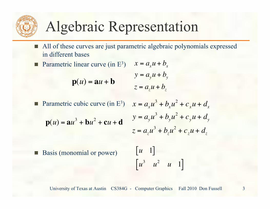
Algebraic RepresentationAll of these curves are just parametric algebraic polynomials expressedin different basesParametric linear curve (in E3)
Parametric cubic curve (in E3)
Basis (monomial or power)
!
x = axu3
+ bxu2
+ cxu + dx
y = ayu3
+ byu2
+ cyu + dy
z = azu3
+ bzu2
+ czu + dz
!
x = axu + bx
y = ayu + by
z = azu + bz
!
p(u) = au + b
!
p(u) = au3
+ bu2
+ cu + d
!
u 1[ ]
u3
u2
u 1[ ]
University of Texas at Austin CS384G - Computer Graphics Fall 2010 Don Fussell 4
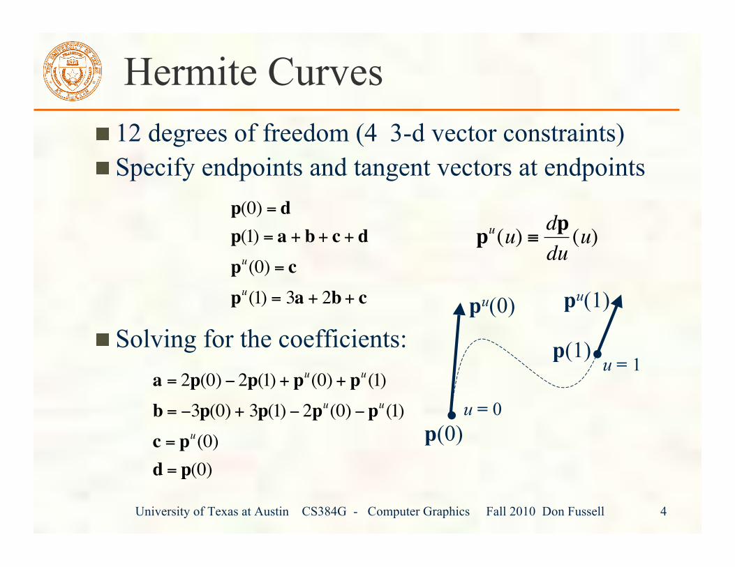
Hermite Curves12 degrees of freedom (4 3-d vector constraints)Specify endpoints and tangent vectors at endpoints
Solving for the coefficients:!
p(0) = d
p(1) = a + b+ c + d
pu(0) = c
pu(1) = 3a + 2b+ c
!
a = 2p(0) " 2p(1) + pu(0) + p
u(1)
b = "3p(0) + 3p(1) " 2pu(0) "p
u(1)
c = pu(0)
d = p(0)
!
pu(u) "
dp
du(u)
•
•pu(0)
u = 0
u = 1
p(0)
p(1)
pu(1)
University of Texas at Austin CS384G - Computer Graphics Fall 2010 Don Fussell 5
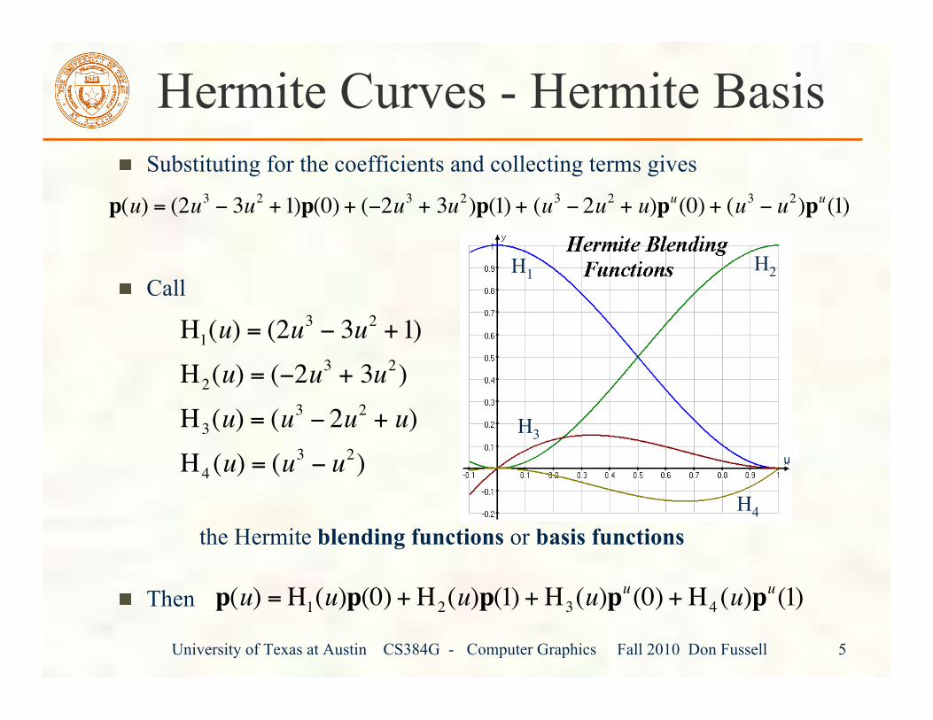
Hermite Curves - Hermite BasisSubstituting for the coefficients and collecting terms gives
Call
the Hermite blending functions or basis functions
Then
!
p(u) = (2u3" 3u
2+1)p(0) + ("2u
3+ 3u
2)p(1) + (u
3" 2u
2+ u)p
u(0) + (u
3" u
2)p
u(1)
!
H1(u) = (2u
3" 3u
2+1)
H2(u) = ("2u
3+ 3u
2)
H3(u) = (u
3" 2u
2+ u)
H4(u) = (u
3" u
2)
!
p(u) =H1(u)p(0) +H
2(u)p(1) +H
3(u)p
u(0) +H
4(u)p
u(1)
H1 H2
H3
H4
n
University of Texas at Austin CS384G - Computer Graphics Fall 2010 Don Fussell 6
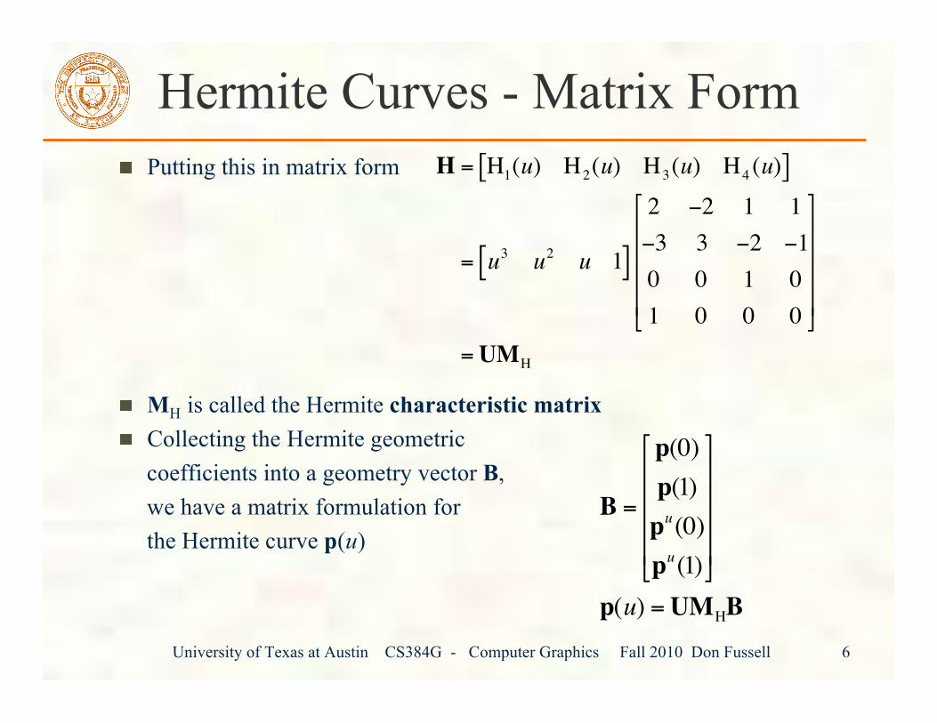
Hermite Curves - Matrix FormPutting this in matrix form
MH is called the Hermite characteristic matrixCollecting the Hermite geometriccoefficients into a geometry vector B,we have a matrix formulation forthe Hermite curve p(u)
!
H = H1(u) H
2(u) H
3(u) H
4(u)[ ]
= u3
u2
u 1[ ]
2 "2 1 1
"3 3 "2 "1
0 0 1 0
1 0 0 0
#
$
% % % %
&
'
( ( ( (
=UMH
!
B =
p(0)
p(1)
pu(0)
pu(1)
"
#
$ $ $ $
%
&
' ' ' '
p(u) =UMHB
University of Texas at Austin CS384G - Computer Graphics Fall 2010 Don Fussell 7
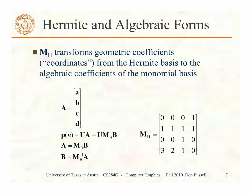
Hermite and Algebraic Forms
MH transforms geometric coefficients(“coordinates”) from the Hermite basis to thealgebraic coefficients of the monomial basis
!
A =
a
b
c
d
"
#
$ $ $ $
%
&
' ' ' '
p(u) =UA =UMHB
A =MHB
B =MH
(1A
!
MH
"1=
0 0 0 1
1 1 1 1
0 0 1 0
3 2 1 0
#
$
% % % %
&
'
( ( ( (
University of Texas at Austin CS384G - Computer Graphics Fall 2010 Don Fussell 8
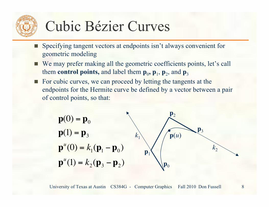
Cubic Bézier CurvesSpecifying tangent vectors at endpoints isn’t always convenient forgeometric modelingWe may prefer making all the geometric coefficients points, let’s callthem control points, and label them p0, p1, p2, and p3
For cubic curves, we can proceed by letting the tangents at theendpoints for the Hermite curve be defined by a vector between a pairof control points, so that:
!
p(0) = p0
p(1) = p3
pu(0) = k
1(p1"p
0)
pu(1) = k
2(p
3"p
2) p0
p1
p2
• p3p(u)
k2
k1
University of Texas at Austin CS384G - Computer Graphics Fall 2010 Don Fussell 9
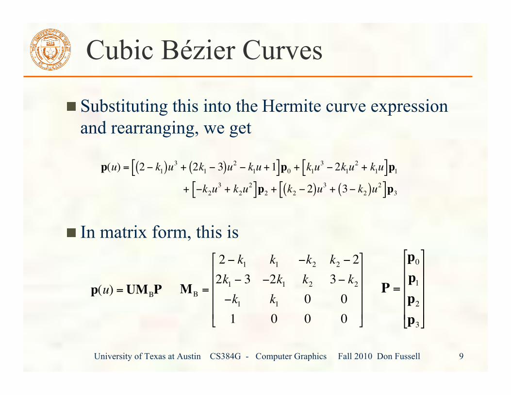
Cubic Bézier Curves
Substituting this into the Hermite curve expressionand rearranging, we get
In matrix form, this is!
p(u) = 2 " k1( )u3 + 2k
1" 3( )u2 " k1u +1[ ]p0 + k
1u3" 2k
1u2 + k
1u[ ]p1
+ "k2u3 + k
2u2[ ]p2 + k
2" 2( )u3 + 3" k
2( )u2[ ]p3
!
p(u) =UMBP
!
MB
=
2 " k1
k1
"k2
k2" 2
2k1" 3 "2k
1k2
3" k2
"k1
k1
0 0
1 0 0 0
#
$
% % % %
&
'
( ( ( (
!
P =
p0
p1
p2
p3
"
#
$ $ $ $
%
&
' ' ' '
University of Texas at Austin CS384G - Computer Graphics Fall 2010 Don Fussell 10
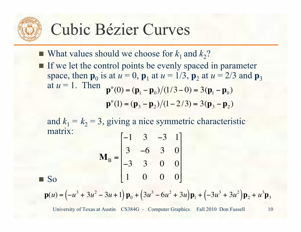
Cubic Bézier CurvesWhat values should we choose for k1 and k2?If we let the control points be evenly spaced in parameterspace, then p0 is at u = 0, p1 at u = 1/3, p2 at u = 2/3 and p3at u = 1. Then
and k1 = k2 = 3, giving a nice symmetric characteristicmatrix:
So
!
MB
=
"1 3 "3 1
3 "6 3 0
"3 3 0 0
1 0 0 0
#
$
% % % %
&
'
( ( ( (
!
p(u) = "u3 + 3u2 " 3u +1( ) p0 + 3u
3" 6u
2 + 3u( )p1 + "3u3 + 3u2( )p2 + u3p3
!
pu(0) = (p
1"p
0) (1/3" 0) = 3(p
1"p
0)
pu(1) = (p
3"p
2) (1" 2 /3) = 3(p
3"p
2)
University of Texas at Austin CS384G - Computer Graphics Fall 2010 Don Fussell 11
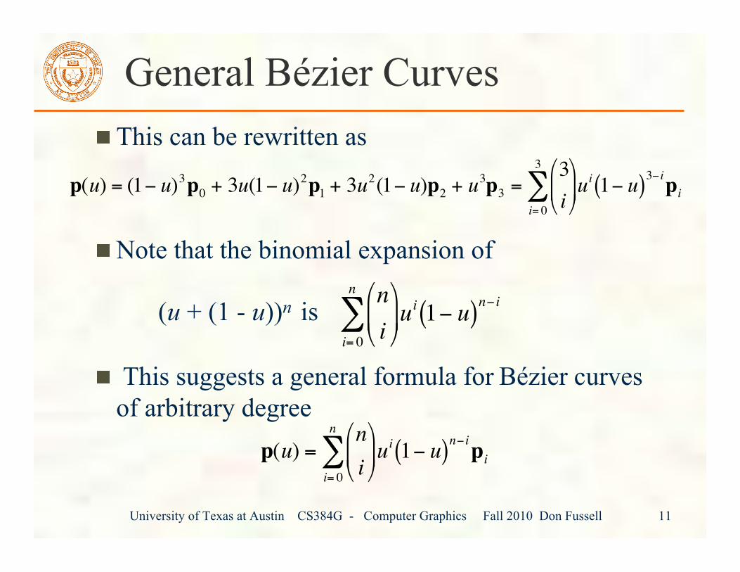
General Bézier CurvesThis can be rewritten as
Note that the binomial expansion of
(u + (1 - u))n is
This suggests a general formula for Bézier curvesof arbitrary degree
!
p(u) = (1" u)3p0
+ 3u(1" u)2p1
+ 3u2(1" u)p2
+ u3p3
=3
i
#
$ % &
' ( u
i1" u( )
3" ipi
i= 0
3
)
!
n
i
"
# $ %
& ' u
i1( u( )
n( i
i= 0
n
)
!
p(u) =n
i
"
# $ %
& ' u
i1( u( )
n( ipi
i= 0
n
)
University of Texas at Austin CS384G - Computer Graphics Fall 2010 Don Fussell 12
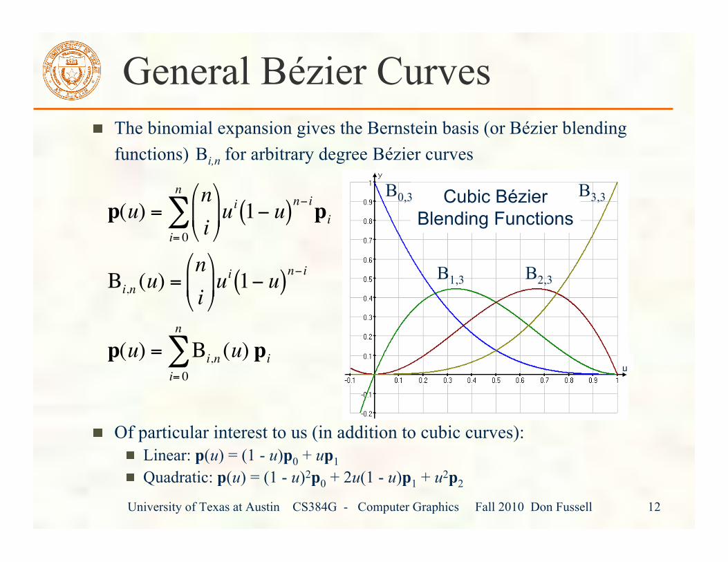
General Bézier CurvesThe binomial expansion gives the Bernstein basis (or Bézier blendingfunctions) Bi,n for arbitrary degree Bézier curves
Of particular interest to us (in addition to cubic curves):Linear: p(u) = (1 - u)p0 + up1Quadratic: p(u) = (1 - u)2p0 + 2u(1 - u)p1 + u2p2
!
p(u) =n
i
"
# $ %
& ' u
i1( u( )
n( ipi
i= 0
n
)
Bi,n(u) =
n
i
"
# $ %
& ' u
i1( u( )
n( i
p(u) = Bi,n(u) p
i
i= 0
n
)
Cubic BézierBlending Functions
B0,3
B1,3 B2,3
B3,3n
University of Texas at Austin CS384G - Computer Graphics Fall 2010 Don Fussell 13
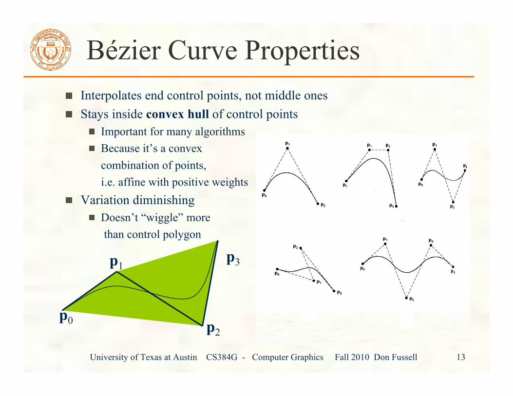
Bézier Curve PropertiesInterpolates end control points, not middle onesStays inside convex hull of control points
Important for many algorithmsBecause it’s a convexcombination of points,i.e. affine with positive weights
Variation diminishingDoesn’t “wiggle” more than control polygon
p0
p1
p2
p3
University of Texas at Austin CS384G - Computer Graphics Fall 2010 Don Fussell 14
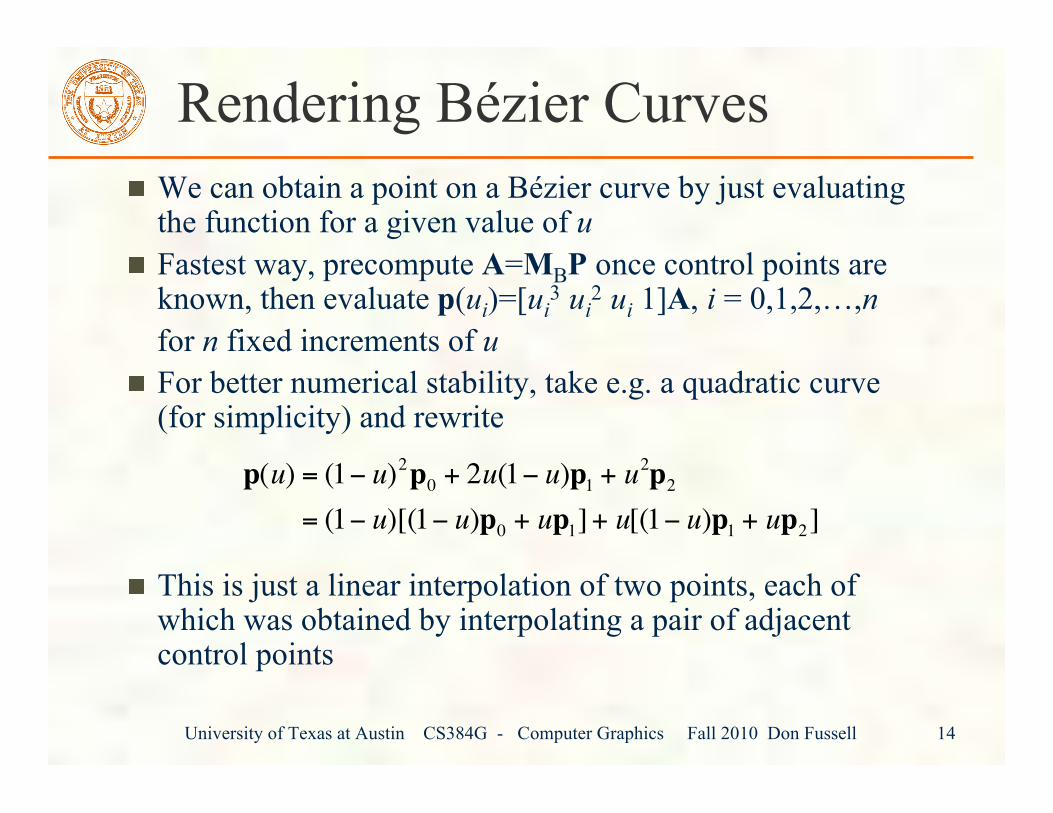
Rendering Bézier CurvesWe can obtain a point on a Bézier curve by just evaluatingthe function for a given value of uFastest way, precompute A=MBP once control points areknown, then evaluate p(ui)=[ui
3 ui2 ui 1]A, i = 0,1,2,…,n
for n fixed increments of uFor better numerical stability, take e.g. a quadratic curve(for simplicity) and rewrite
This is just a linear interpolation of two points, each ofwhich was obtained by interpolating a pair of adjacentcontrol points!
p(u) = (1" u)2p0
+ 2u(1" u)p1+ u
2p2
= (1" u)[(1" u)p0
+ up1]+ u[(1" u)p
1+ up
2]
University of Texas at Austin CS384G - Computer Graphics Fall 2010 Don Fussell 15
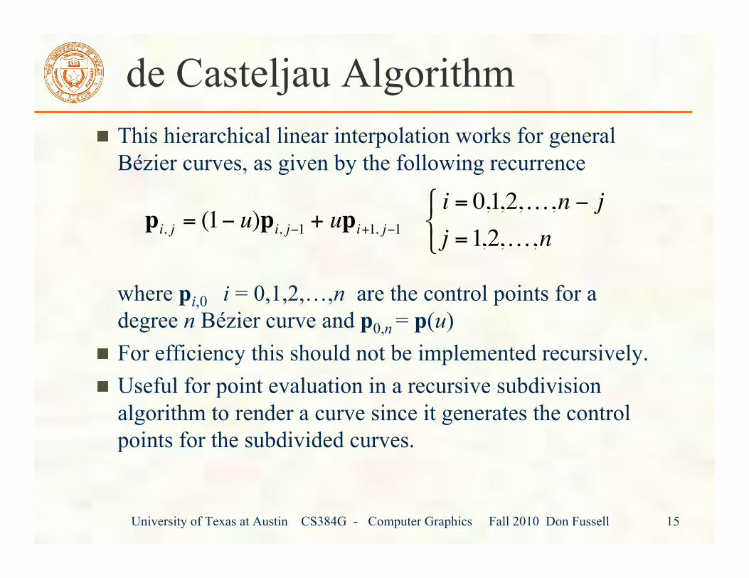
de Casteljau AlgorithmThis hierarchical linear interpolation works for generalBézier curves, as given by the following recurrence
where pi,0 i = 0,1,2,…,n are the control points for adegree n Bézier curve and p0,n = p(u)For efficiency this should not be implemented recursively.Useful for point evaluation in a recursive subdivisionalgorithm to render a curve since it generates the controlpoints for the subdivided curves.
!
pi, j = (1" u)pi, j"1 + upi+1, j"1i = 0,1,2,K,n " j
j =1,2,K,n
# $ %
University of Texas at Austin CS384G - Computer Graphics Fall 2010 Don Fussell 16
de Casteljau Algorithm
p0
p1
p2
p3
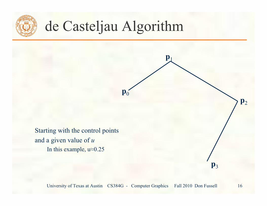
Starting with the control pointsand a given value of u
In this example, u≈0.25
University of Texas at Austin CS384G - Computer Graphics Fall 2010 Don Fussell 17
de Casteljau Algorithm
p0
q0
p1
p2
p3
q2
q1
!
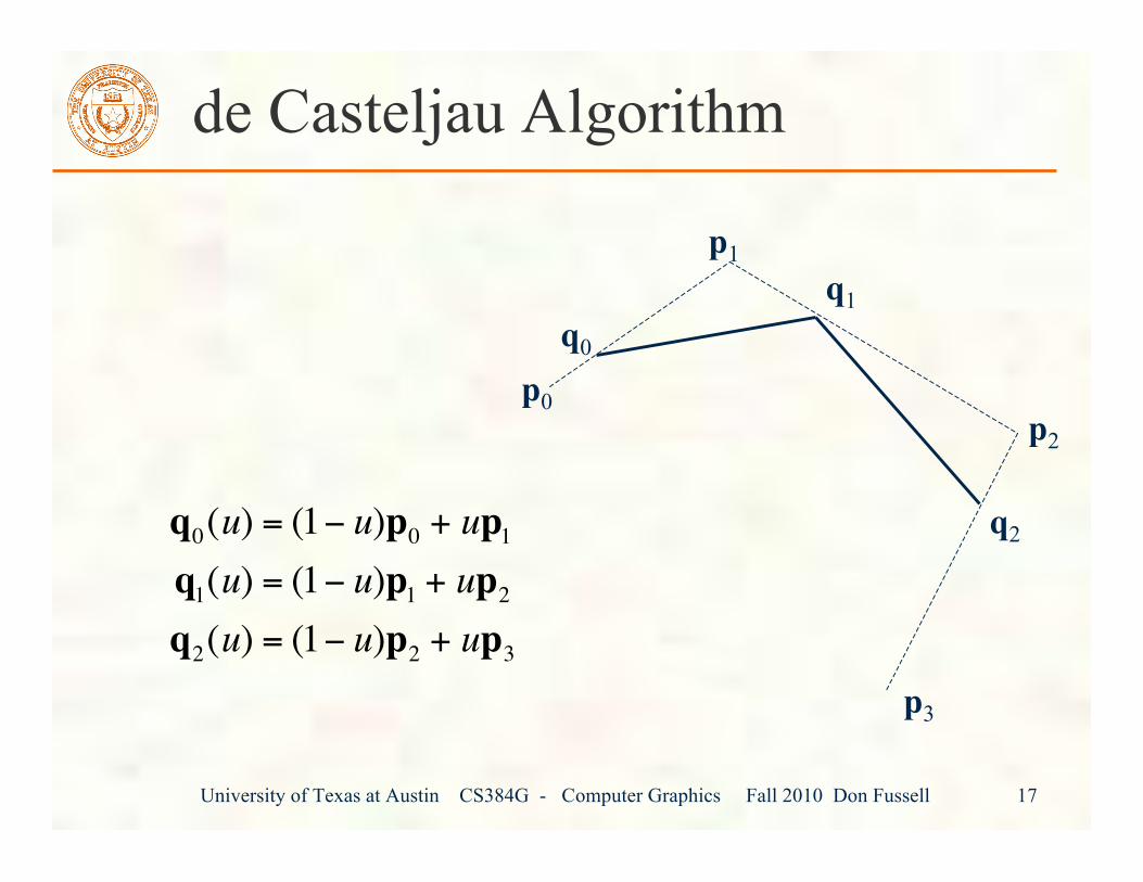
q0(u) = (1" u)p
0+ up
1
q1(u) = (1" u)p
1+ up
2
q2(u) = (1" u)p
2+ up
3
University of Texas at Austin CS384G - Computer Graphics Fall 2010 Don Fussell 18
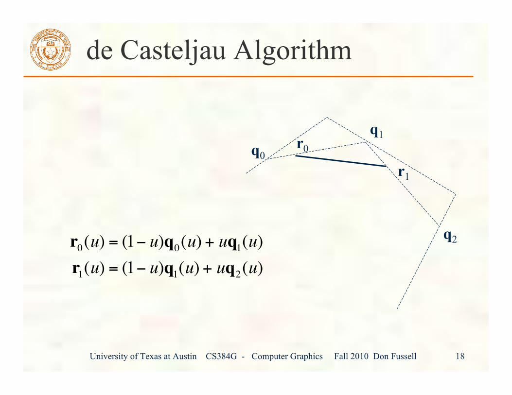
de Casteljau Algorithm
q0
q2
q1
r1
r0
!
r0(u) = (1" u)q
0(u) + uq
1(u)
r1(u) = (1" u)q
1(u) + uq
2(u)
University of Texas at Austin CS384G - Computer Graphics Fall 2010 Don Fussell 19
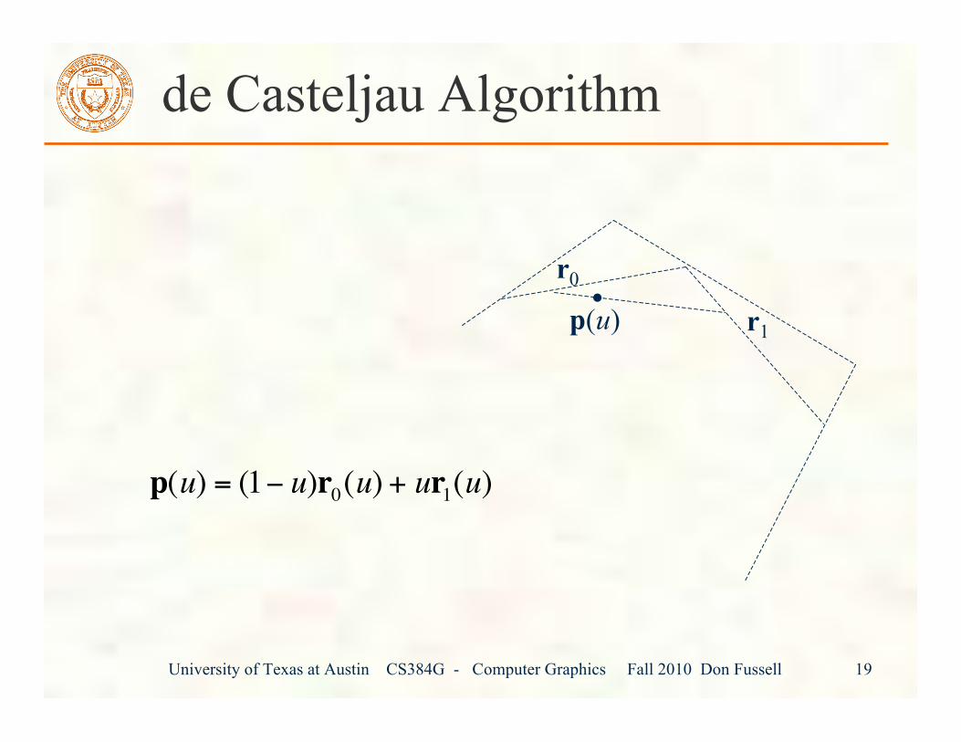
de Casteljau Algorithm
r1p(u)
r0•
!
p(u) = (1" u)r0(u) + ur
1(u)
University of Texas at Austin CS384G - Computer Graphics Fall 2010 Don Fussell 20
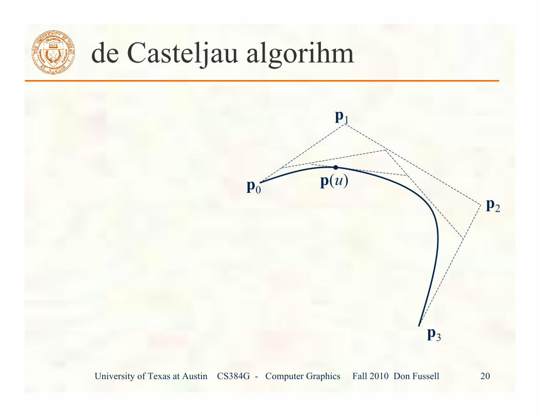
de Casteljau algorihm
•p0
p1
p2
p3
p(u)
University of Texas at Austin CS384G - Computer Graphics Fall 2010 Don Fussell 21
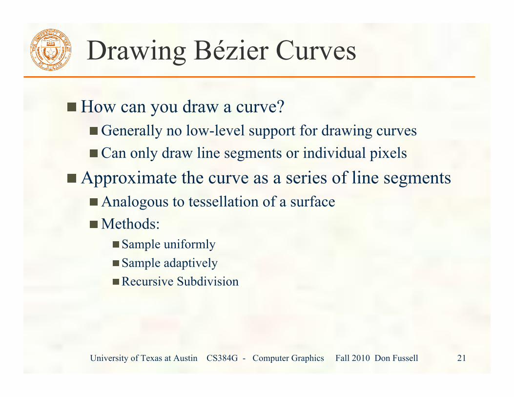
Drawing Bézier Curves
How can you draw a curve?Generally no low-level support for drawing curvesCan only draw line segments or individual pixels
Approximate the curve as a series of line segmentsAnalogous to tessellation of a surfaceMethods:
Sample uniformlySample adaptivelyRecursive Subdivision
University of Texas at Austin CS384G - Computer Graphics Fall 2010 Don Fussell 22
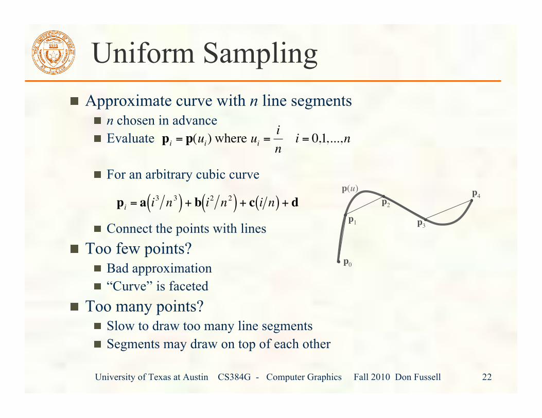
Uniform SamplingApproximate curve with n line segments
n chosen in advanceEvaluate
For an arbitrary cubic curve
Connect the points with linesToo few points?
Bad approximation“Curve” is faceted
Too many points?Slow to draw too many line segmentsSegments may draw on top of each other
p4
p0
p1
p2
p3
p(u)
!
pi= p(u
i) where u
i=i
ni = 0,1,...,n
!
pi= a i3 n3( ) + b i2 n2( ) + c i n( ) + d
University of Texas at Austin CS384G - Computer Graphics Fall 2010 Don Fussell 23
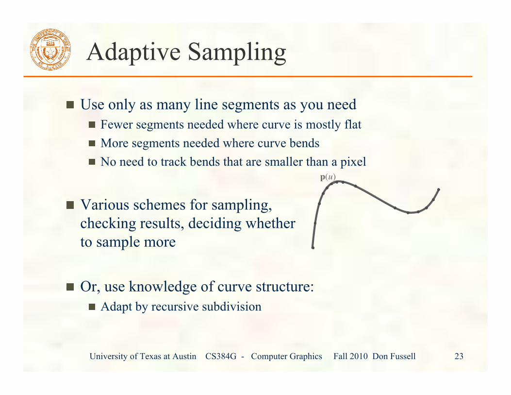
Adaptive Sampling
Use only as many line segments as you needFewer segments needed where curve is mostly flatMore segments needed where curve bendsNo need to track bends that are smaller than a pixel
Various schemes for sampling,checking results, deciding whetherto sample more
Or, use knowledge of curve structure:Adapt by recursive subdivision
p(u)

University of Texas at Austin CS384G - Computer Graphics Fall 2010 Don Fussell 24
Recursive Subdivision
Any cubic curve segment can be expressed as aBézier curveAny piece of a cubic curve is itself a cubic curveTherefore:
Any Bézier curve can be broken up into smaller BéziercurvesBut how…?
University of Texas at Austin CS384G - Computer Graphics Fall 2010 Don Fussell 25
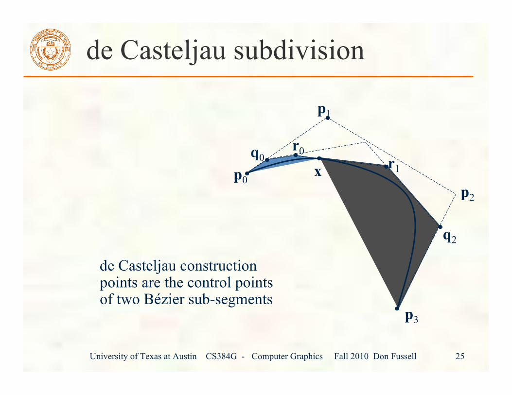
de Casteljau constructionpoints are the control pointsof two Bézier sub-segments
xp0
p1
p2
p3
de Casteljau subdivision
q0r0
r1
q2
University of Texas at Austin CS384G - Computer Graphics Fall 2010 Don Fussell 26
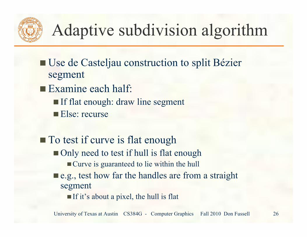
Adaptive subdivision algorithm
Use de Casteljau construction to split BéziersegmentExamine each half:
If flat enough: draw line segmentElse: recurse
To test if curve is flat enoughOnly need to test if hull is flat enough
Curve is guaranteed to lie within the hulle.g., test how far the handles are from a straightsegment
If it’s about a pixel, the hull is flat
University of Texas at Austin CS384G - Computer Graphics Fall 2010 Don Fussell 27
Composite CurvesHermite and Bézier curves generalize line segments to higher degreepolynomials. But what if we want more complicated curves than wecan get with a single one of these? Then we need to build compositecurves, like polylines but curved.Continuity conditions for composite curves
C0 - The curve is continuous, i.e. the endpoints of consecutive curvesegments coincideC1 - The tangent (derivative with respect to the parameter) is continuous,i.e. the tangents match at the common endpoint of consecutive curvesegmentsC2 - The second parametric derivative is continuous, i.e. matches atcommon endpointsG0 - Same as C0
G1 - Derivatives wrt the coordinates are continuous. Weaker than C1, thetangents should point in the same direction, but lengths can differ.G2 - Second derivatives wrt the coordinates are continuous…
University of Texas at Austin CS384G - Computer Graphics Fall 2010 Don Fussell 28
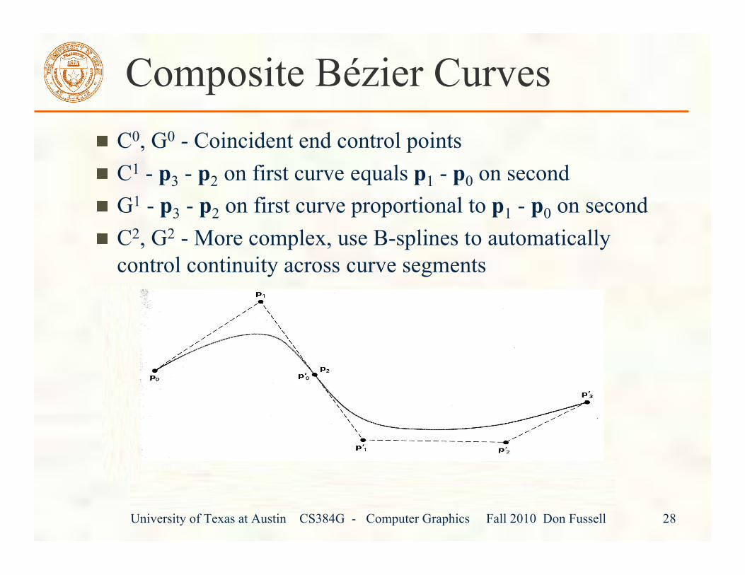
Composite Bézier CurvesC0, G0 - Coincident end control pointsC1 - p3 - p2 on first curve equals p1 - p0 on secondG1 - p3 - p2 on first curve proportional to p1 - p0 on secondC2, G2 - More complex, use B-splines to automaticallycontrol continuity across curve segments
University of Texas at Austin CS384G - Computer Graphics Fall 2010 Don Fussell 29
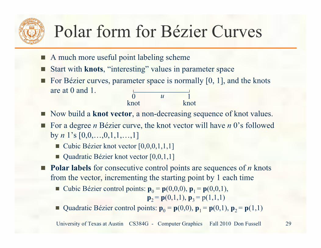
Polar form for Bézier CurvesA much more useful point labeling schemeStart with knots, “interesting” values in parameter spaceFor Bézier curves, parameter space is normally [0, 1], and the knotsare at 0 and 1.
Now build a knot vector, a non-decreasing sequence of knot values.For a degree n Bézier curve, the knot vector will have n 0’s followedby n 1’s [0,0,…,0,1,1,…,1]
Cubic Bézier knot vector [0,0,0,1,1,1]Quadratic Bézier knot vector [0,0,1,1]
Polar labels for consecutive control points are sequences of n knotsfrom the vector, incrementing the starting point by 1 each time
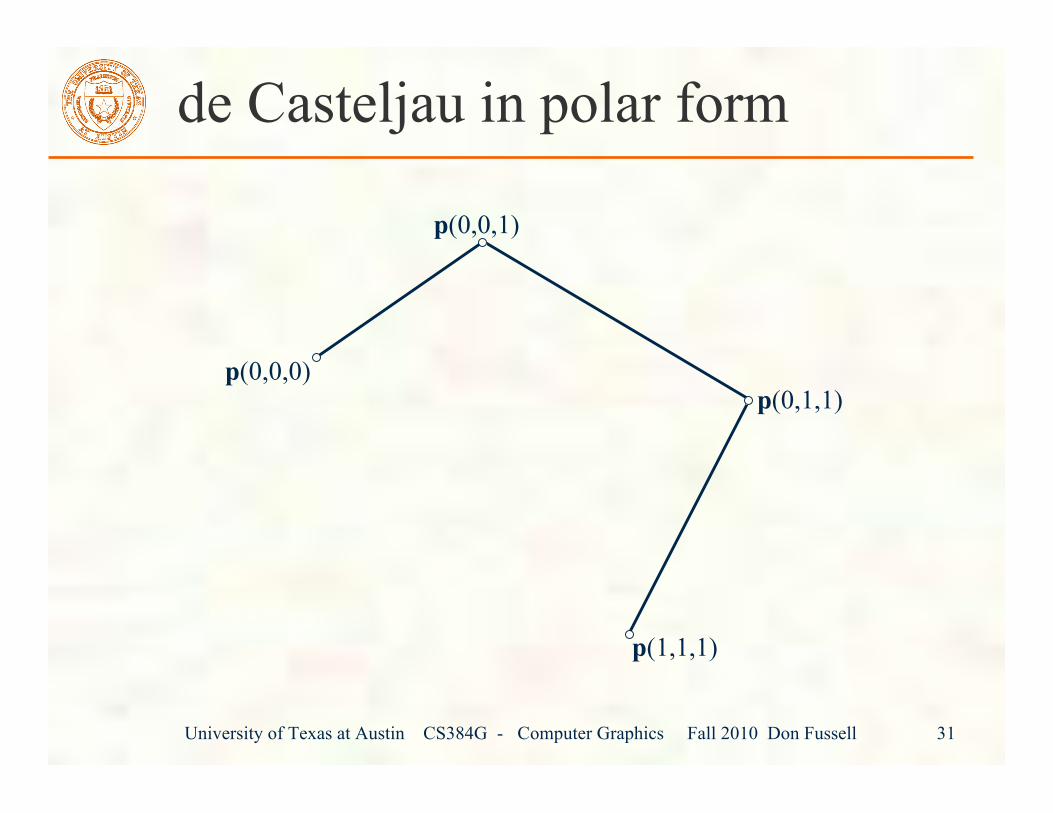
Cubic Bézier control points: p0 = p(0,0,0), p1 = p(0,0,1), p2 = p(0,1,1), p3 = p(1,1,1)
Quadratic Bézier control points: p0 = p(0,0), p1 = p(0,1), p2 = p(1,1)
u0 1knot knot
University of Texas at Austin CS384G - Computer Graphics Fall 2010 Don Fussell 30
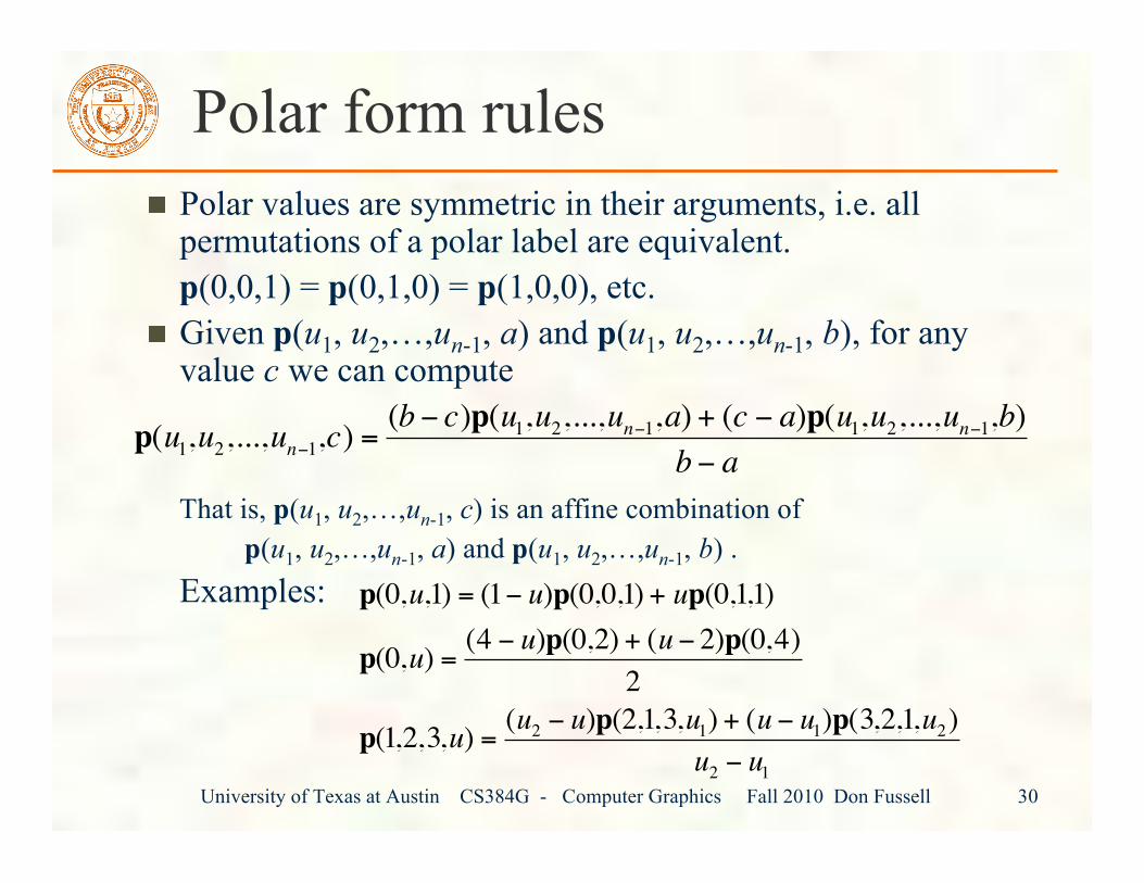
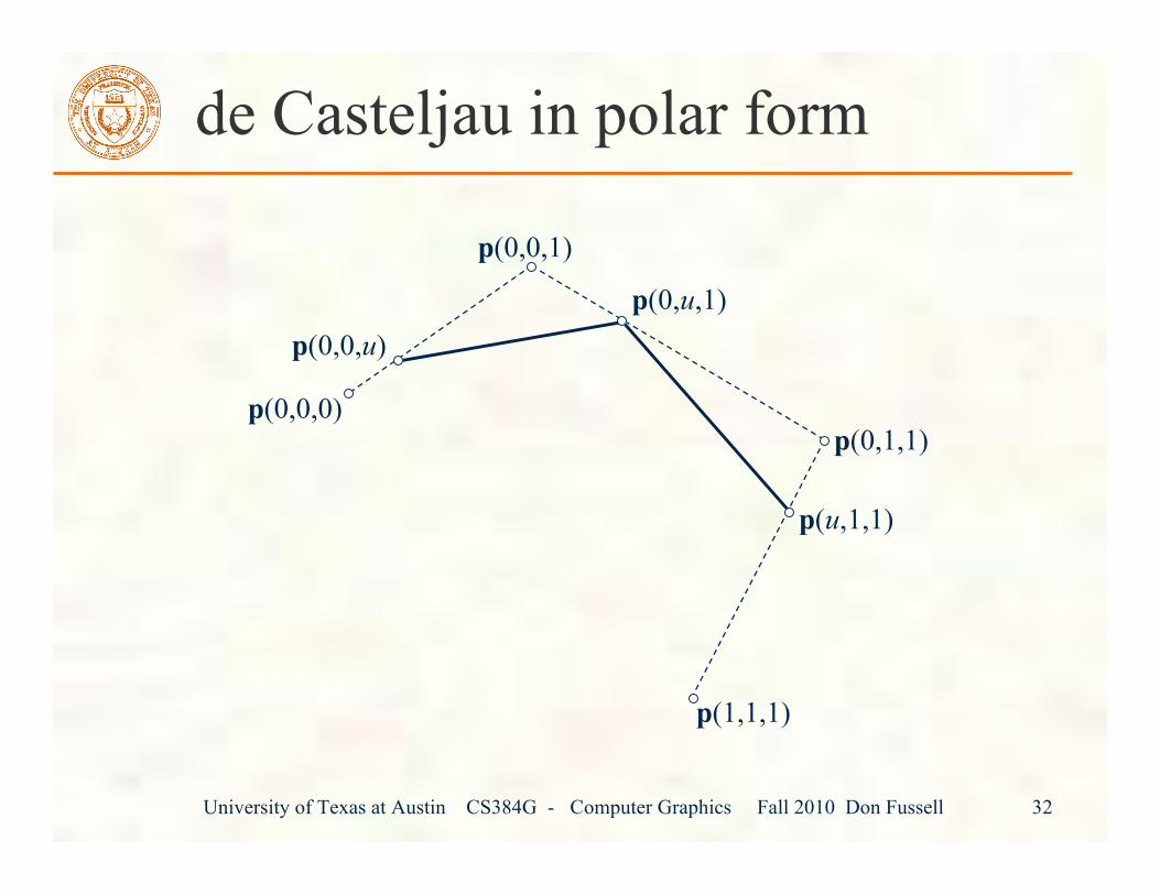
Polar form rulesPolar values are symmetric in their arguments, i.e. allpermutations of a polar label are equivalent.p(0,0,1) = p(0,1,0) = p(1,0,0), etc.Given p(u1, u2,…,un-1, a) and p(u1, u2,…,un-1, b), for anyvalue c we can compute
That is, p(u1, u2,…,un-1, c) is an affine combination ofp(u1, u2,…,un-1, a) and p(u1, u2,…,un-1, b) .
Examples:!
p(u1,u2,...,u
n"1,c) =(b " c)p(u
1,u2,...,u
n"1,a) + (c " a)p(u1,u2,...,u
n"1,b)
b " a
!
p(0,u,1) = (1" u)p(0,0,1) + up(0,1,1)
p(0,u) =(4 " u)p(0,2) + (u " 2)p(0,4)
2
p(1,2,3,u) =(u
2" u)p(2,1,3,u
1) + (u " u
1)p(3,2,1,u
2)
u2" u
1
University of Texas at Austin CS384G - Computer Graphics Fall 2010 Don Fussell 31
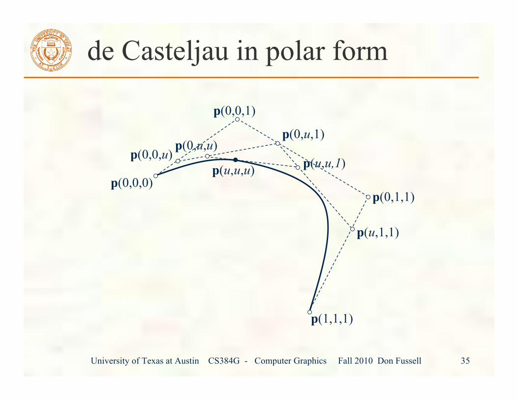
de Casteljau in polar form
p(0,0,0)
p(1,1,1)
p(0,1,1)
p(0,0,1)
University of Texas at Austin CS384G - Computer Graphics Fall 2010 Don Fussell 32
de Casteljau in polar form
p(0,0,0)
p(1,1,1)
p(0,1,1)
p(0,0,1)
p(0,0,u)p(0,u,1)
p(u,1,1)
University of Texas at Austin CS384G - Computer Graphics Fall 2010 Don Fussell 33
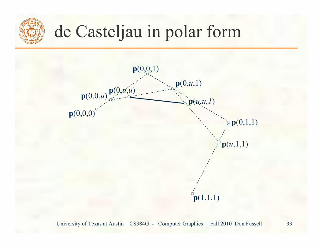
de Casteljau in polar form
p(0,0,0)
p(1,1,1)
p(0,1,1)
p(0,0,1)
p(0,0,u)p(0,u,1)
p(u,1,1)
p(0,u,u)p(u,u,1)
University of Texas at Austin CS384G - Computer Graphics Fall 2010 Don Fussell 34
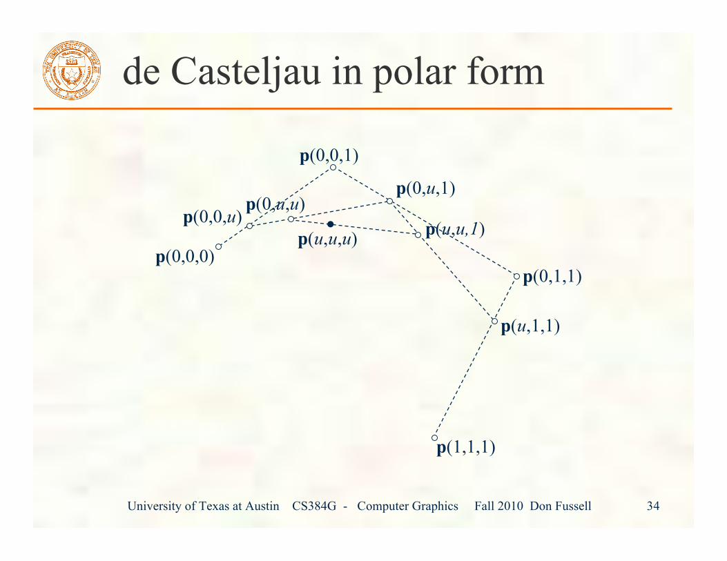
de Casteljau in polar form
p(0,0,0)
p(1,1,1)
p(0,1,1)
p(0,0,1)
p(0,0,u)p(0,u,1)
p(u,1,1)
p(0,u,u)p(u,u,1)•p(u,u,u)
University of Texas at Austin CS384G - Computer Graphics Fall 2010 Don Fussell 35
de Casteljau in polar form
p(0,0,0)
p(1,1,1)
p(0,1,1)
p(0,0,1)
p(0,0,u)p(0,u,1)
p(u,1,1)
p(0,u,u)p(u,u,1)•p(u,u,u)
University of Texas at Austin CS384G - Computer Graphics Fall 2010 Don Fussell 36
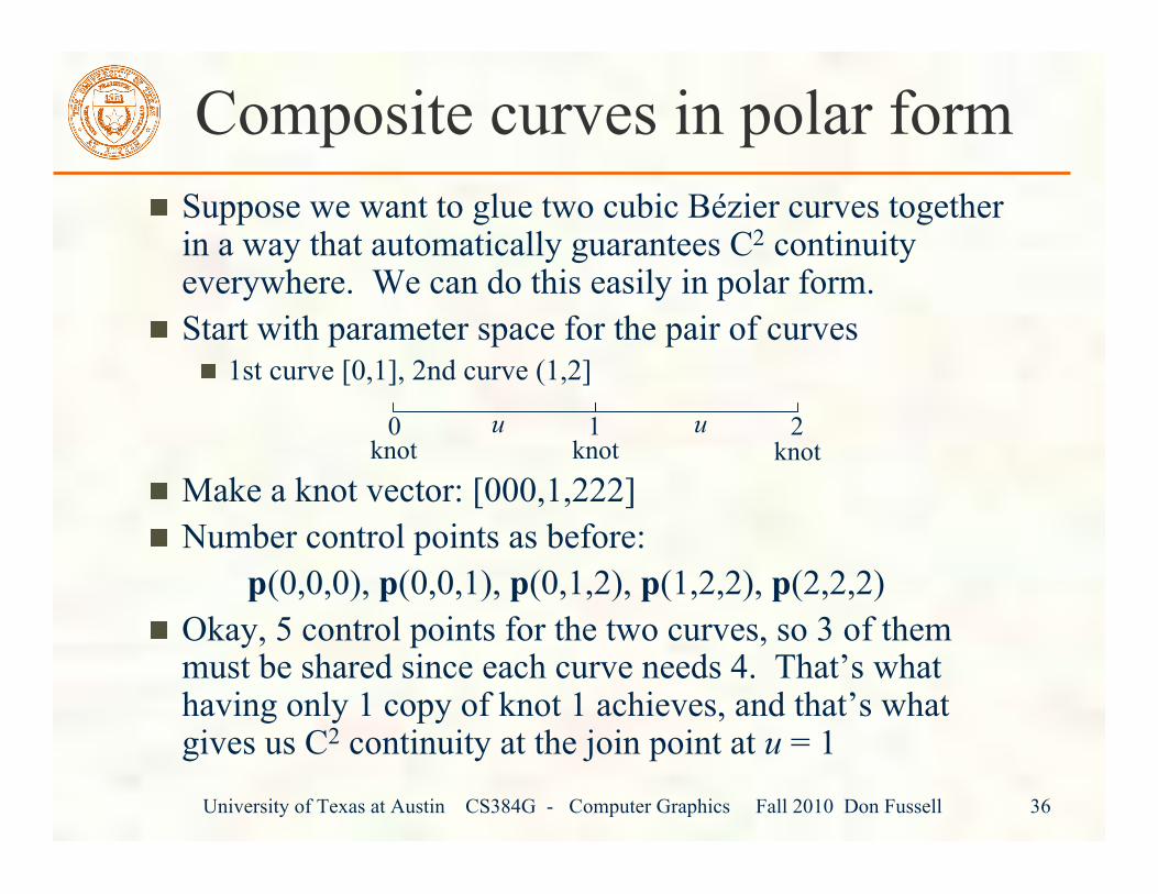
Composite curves in polar formSuppose we want to glue two cubic Bézier curves togetherin a way that automatically guarantees C2 continuityeverywhere. We can do this easily in polar form.Start with parameter space for the pair of curves
1st curve [0,1], 2nd curve (1,2]
Make a knot vector: [000,1,222]Number control points as before:
p(0,0,0), p(0,0,1), p(0,1,2), p(1,2,2), p(2,2,2)Okay, 5 control points for the two curves, so 3 of themmust be shared since each curve needs 4. That’s whathaving only 1 copy of knot 1 achieves, and that’s whatgives us C2 continuity at the join point at u = 1
u0 1knot knot
u 2knot
University of Texas at Austin CS384G - Computer Graphics Fall 2010 Don Fussell 37
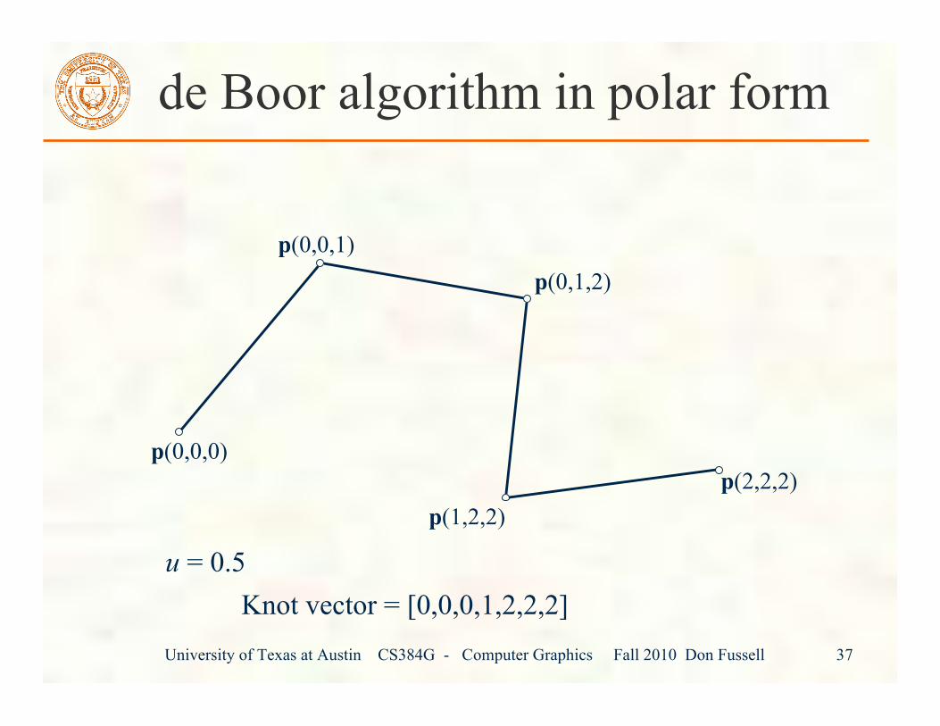
de Boor algorithm in polar form
p(0,0,0)
p(0,0,1)p(0,1,2)
p(1,2,2)p(2,2,2)
u = 0.5Knot vector = [0,0,0,1,2,2,2]
University of Texas at Austin CS384G - Computer Graphics Fall 2010 Don Fussell 38
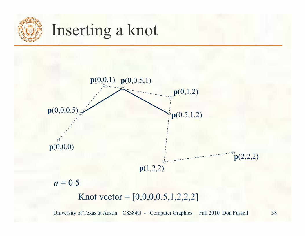
Inserting a knot
p(0,0,0)
p(0,0,1)p(0,1,2)
p(1,2,2)p(2,2,2)
u = 0.5
p(0,0,0.5)
p(0,0.5,1)
p(0.5,1,2)
Knot vector = [0,0,0,0.5,1,2,2,2]
University of Texas at Austin CS384G - Computer Graphics Fall 2010 Don Fussell 39
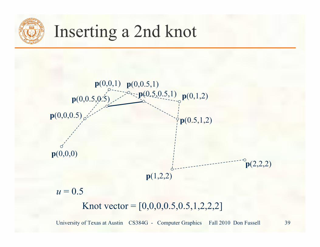
Inserting a 2nd knot
p(0,0,0)
p(0,0,1)p(0,1,2)
p(1,2,2)p(2,2,2)
u = 0.5
p(0,0,0.5)
p(0,0.5,1)
p(0.5,1,2)
p(0,0.5,0.5) p(0.5,0.5,1)
Knot vector = [0,0,0,0.5,0.5,1,2,2,2]
University of Texas at Austin CS384G - Computer Graphics Fall 2010 Don Fussell 40
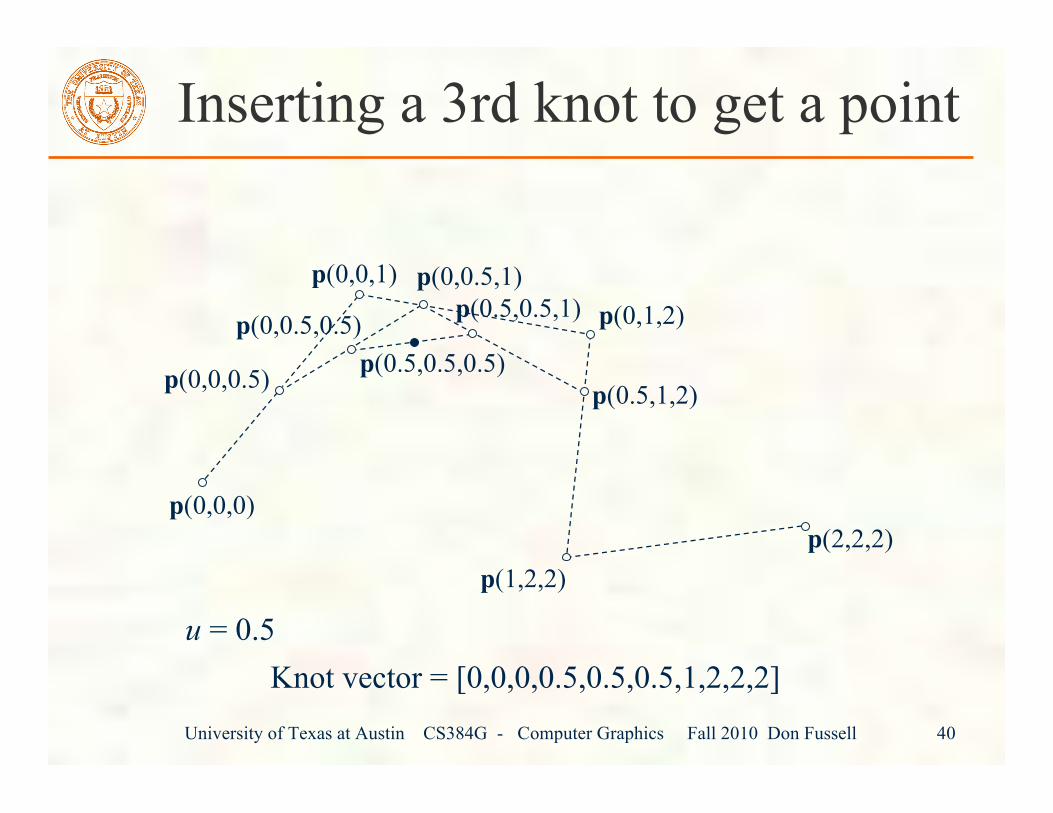
Inserting a 3rd knot to get a point
p(0,0,0)
p(0,0,1)p(0,1,2)
p(1,2,2)p(2,2,2)
u = 0.5
p(0,0,0.5)
p(0,0.5,1)
p(0.5,1,2)
p(0,0.5,0.5) p(0.5,0.5,1)
p(0.5,0.5,0.5)
Knot vector = [0,0,0,0.5,0.5,0.5,1,2,2,2]
University of Texas at Austin CS384G - Computer Graphics Fall 2010 Don Fussell 41
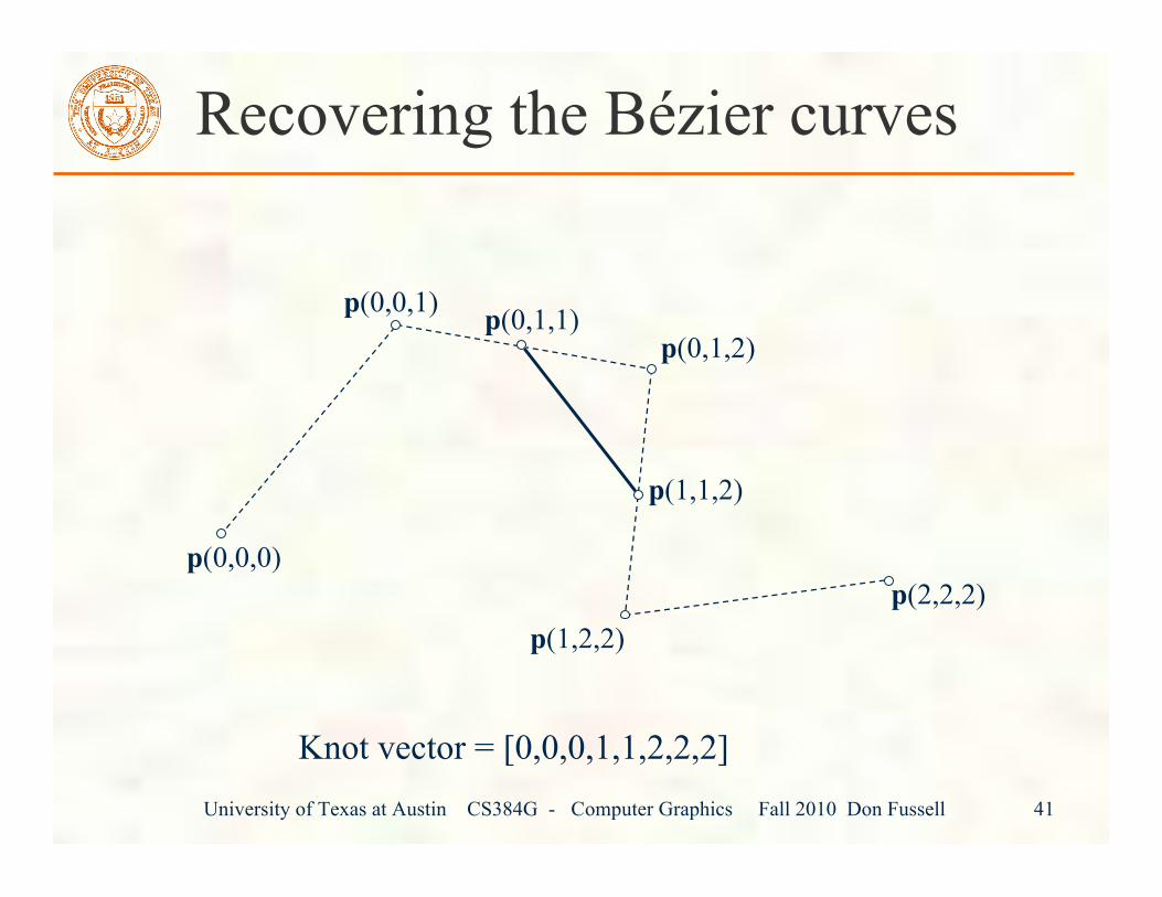
Recovering the Bézier curves
p(0,0,0)
p(0,0,1)p(0,1,2)
p(1,2,2)p(2,2,2)
Knot vector = [0,0,0,1,1,2,2,2]
p(0,1,1)
p(1,1,2)
University of Texas at Austin CS384G - Computer Graphics Fall 2010 Don Fussell 42
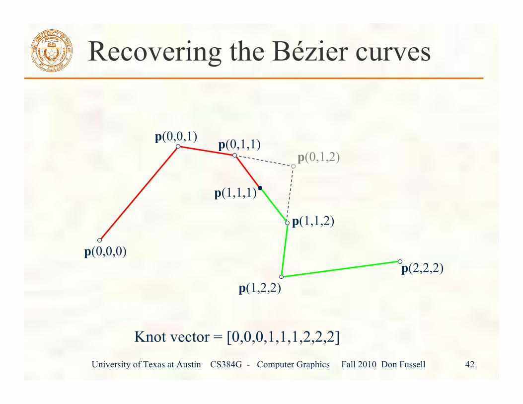
Recovering the Bézier curves
p(0,0,0)
p(0,0,1)p(0,1,2)
p(1,2,2)p(2,2,2)
Knot vector = [0,0,0,1,1,1,2,2,2]
p(0,1,1)
p(1,1,2)
p(1,1,1)
University of Texas at Austin CS384G - Computer Graphics Fall 2010 Don Fussell 43
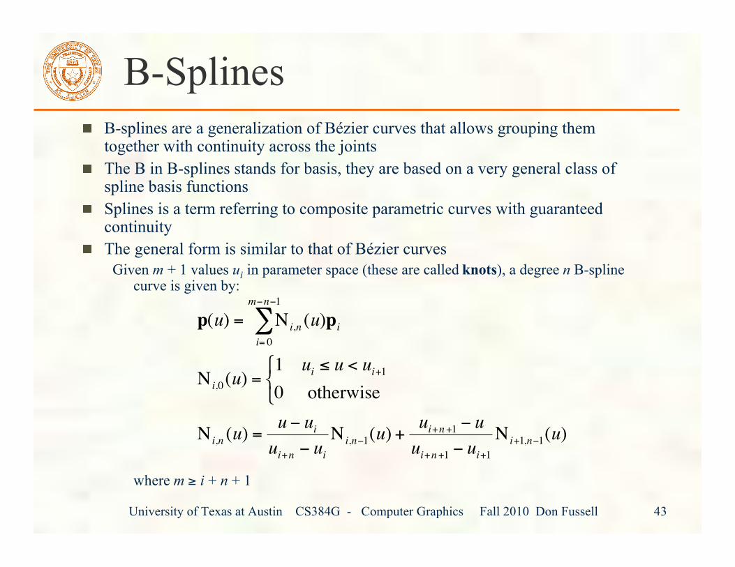
B-SplinesB-splines are a generalization of Bézier curves that allows grouping themtogether with continuity across the jointsThe B in B-splines stands for basis, they are based on a very general class ofspline basis functionsSplines is a term referring to composite parametric curves with guaranteedcontinuityThe general form is similar to that of Bézier curves
Given m + 1 values ui in parameter space (these are called knots), a degree n B-splinecurve is given by:
where m ≥ i + n + 1
!
p(u) = Ni,n (u)pi
i= 0
m"n"1
#
Ni,0 (u) =
1 ui$ u < u
i+1
0 otherwise
% & '
Ni,n (u) =
u " ui
ui+n " ui
Ni,n"1(u) +
ui+n+1 " u
ui+n+1 " ui+1
Ni+1,n"1(u)
University of Texas at Austin CS384G - Computer Graphics Fall 2010 Don Fussell 44
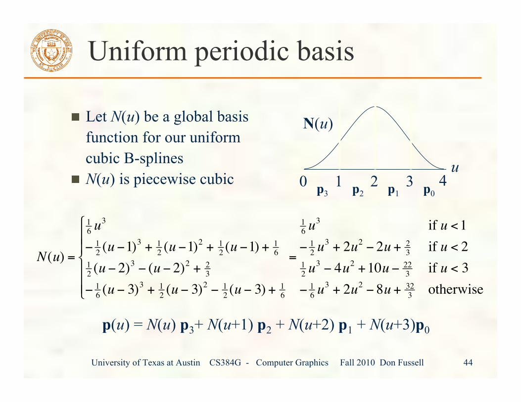
Uniform periodic basis
Let N(u) be a global basisfunction for our uniformcubic B-splinesN(u) is piecewise cubic
p(u) = N(u) p3+ N(u+1) p2 + N(u+2) p1 + N(u+3)p0
0 4u
N(u)
!
N(u) =
1
6u
3
" 1
2(u "1)
3+ 1
2(u "1)
2+ 1
2(u "1) + 1
6
1
2(u " 2)
3 " (u " 2)2
+ 2
3
" 1
6(u " 3)
3+ 1
2(u " 3)
2 " 1
2(u " 3) + 1
6
=
1
6u
3if u <1
" 1
2u
3+ 2u
2 " 2u + 2
3if u < 2
1
2u
3 " 4u2
+10u " 22
3if u < 3
" 1
6u
3+ 2u
2 " 8u + 32
3otherwise
#
$
% %
&
% %
1 2 3 p0p1p2p3
University of Texas at Austin CS384G - Computer Graphics Fall 2010 Don Fussell 45
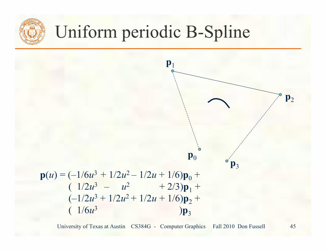
Uniform periodic B-Spline
p0
p1
p2
p3p(u) = (–1/6u3 + 1/2u2 – 1/2u + 1/6)p0 +
( 1/2u3 – u2 + 2/3)p1 +
(–1/2u3 + 1/2u2 + 1/2u + 1/6)p2 +
( 1/6u3 )p3