Parametric Empirical Bayes Inference: Theory and ... & Francis, Ltd. and American Statistical Association are collaborating with JSTOR to digitize, preserve and extend access to Journal

Taylor & Francis, Ltd. and American Statistical Association are collaborating with JSTOR to digitize, preserve and extend access to Journal of the American Statistical Association.

http://www.jstor.org

Parametric Empirical Bayes Inference: Theory and Applications Author(s): Carl N. Morris Source: Journal of the American Statistical Association, Vol. 78, No. 381 (Mar., 1983), pp. 47-55Published by: on behalf of the Taylor & Francis, Ltd. American Statistical AssociationStable URL: http://www.jstor.org/stable/2287098Accessed: 04-11-2015 01:57 UTC

Your use of the JSTOR archive indicates your acceptance of the Terms & Conditions of Use, available at http://www.jstor.org/page/ info/about/policies/terms.jsp

JSTOR is a not-for-profit service that helps scholars, researchers, and students discover, use, and build upon a wide range of content in a trusted digital archive. We use information technology and tools to increase productivity and facilitate new forms of scholarship. For more information about JSTOR, please contact [email protected].

This content downloaded from 128.173.127.127 on Wed, 04 Nov 2015 01:57:53 UTCAll use subject to JSTOR Terms and Conditions

http://www.jstor.org

http://www.jstor.org/action/showPublisher?publisherCode=taylorfrancis

http://www.jstor.org/action/showPublisher?publisherCode=astata

http://www.jstor.org/stable/2287098

http://www.jstor.org/page/info/about/policies/terms.jsp



Parametric Empirical Bayes Inference: Theory and Applications

CARL N. MORRIS*

This article reviews the state of multiparameter shrinkage estimators with emphasis on the empirical Bayes viewpoint, particularly in the case of parametric prior distributions. Some successful applications of major impor- tance are considered. Recent results concerning estimates of error and confidence intervals are described and illustrated with data.

KEY WORDS: Empirical Bayes; Parametric empirical Bayes; Empirical Bayes confidence intervals; Stein's estimator.

1. MULTIPARAMETER ESTIMATION: -BORROWING STRENGTH FROM THE ENSEMBLE

Statisticians often must make many estimates of similar quantities, for example, estimates of annual income must be made for many areas, the quality of a process must be re-evaluated every month, an actuary must estimate the risks of many different groups of drivers, and so on. Thus, the situation of Table 1 often arises.

We assume that k parameters 01, . . . , ok must be estimated starting with independent unbiased estimates Y1, .. ., Yk, EYi = Oi. In cases where Yi is normal we can write

Yi I Oi-N(%i, Vi), i = 1, . . ,k independently (1.1)

with Vi = var( Yi). The estimate Yi often would be a re- duction of the original data, perhaps a sample mean or some other statistic, each computed from an independent set of data. We will take the variances Vi to be known here, in order to concentrate on the main issues. Usually, however, they would have to be estimated, perhaps by the within-groups sums of squares.

If the Vi are suitably small, the statistician may be content to use the estimates Yi, but otherwise he may seek alternative estimates 0i of Oi. Examples include i =Y, the grand mean, or more generally,

6i= z1tb, (1.2)

* Carl N. Morris is Professor, Department of Mathematics, Univer- sity of Texas, Austin, TX 78712. This paper was presented at the August 16-19, 1982 meeting of the American Statistical Association, Cincinnati, Ohio, as a General Methodology Lecture. The author wishes to acknowledge interdependence between the ideas expressed here and those of his longstanding empirical Bayes collaborator, Bradley Efron, but without implying Dr. Efron's acceptance of all the paper's declarations. Research supported by the National Science Foundation under Grant MCS-8104-250.

with zi an r-dimensional column vector of regression variables, and b a vector of estimated regression coefficients. We assume 0 < r - k - 3 throughout (this is required, for example, so that the expectations in (1.4), (1.17) exist and so that (1.19) be positive). The estimates (1.2) would be ideal if one knew that for every i

Oi= z/13. (1.3)

In that case b is computed as the least squares estimator

b = (Z'DZ)'-Z'DY (1.4)

with Z the k x r matrix having rows zi', D- = Diagonal (VI, . . ., Vk), Y = (Y1,. . . , Yk)'. Then 0i is unbiased, and dominates Yi as an estimator of Oi for sum of squared error loss function.

Which estimate of Oi should be preferred if (1.3) is not known to hold? In the most interesting cases a compromise estimator

0i = (1 - Bi)Yi + Bi 6i (1.5)

will outperform either extreme choice. Here Bi is a shrinking coefficient, 0 c Bi ' 1, Bi = 0 resulting in no shrinkage of 0i from Yi towards 0i.

How do we choose the Bi? That depends on the variance A of the errors Oi - zi',. If A = 0 then (1.3) holds and Bi = 1 is best, but Bi should decrease to 0 as A -> oo. Although A is unknown, the Yi values contain information about A that can be used profitably.

This issue can be incorporated formally by making the assumption that

indep

oi I I, Ai - N(zi'I, Ai) i = 1, . . . k (1.6)

to complement the model (1.1). Here, we allow Oi to have a different variance Ai for each i. Many other assumptions might be appropriate for (1.6), that the Oi be dependent, that the Oi be nonnormal, and so on. The complexity of such assumptions must be restricted, however, so the data Y can be used to investigate the model (1.6) and any unknown parameters.

The choice between Yi and 0i as an estimator of Oi is, in terms of (1.6), a choice between Ai = co and Ai = 0, respectively. The model (1.1), (1.6) will lead to better results because it is richer, also allowing values 0 < A < oo. Thus, the superiority of shrinkage estimators like

? Journal of the American Statistical Association March 1983, Volume 78, Number 381

Applications Section

47



48 Journal of the American Statistical Association, March 1983

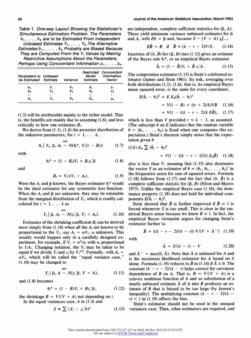
Table 1. One-way Layout Showing the Statistician's Simultaneous Estimation Problem. The Parameters 01, * * *, ok are to be Estimated From Independent Unbiased Estimates Y1, . . ., Yk. The Alternative

Estimates 01, .. ,ok Probably are Biased Because They are Computed From the Y1 Values by Making Restrictive Assumptions About the Parameters,

Perhaps Using Concomitant Information z1, . . ., IZk

Restricted Concomitant Parameters to Unbiased Model Information be Estimated Estimate Variance Estimate Vector

Oi Y, V1 O1 Z1 02 Y2 V2 02 z2

Ok Yk Vk Ok Zk

(1.5) will be attributable mainly to the richer model. That is, the benefits are mainly due to assuming (1.6), and less critically to how one estimates Bi.

We derive from (1. 1), (1.6) the posterior distribution of the unknown parameters, for i = 1, .. .k,

ind

Oi I Yi, , Ai - N(0i*, Vi(I - Bi)) (1.7)

with

Oi*= (1 - Bi)Yi + Bizi' (1.8)

and

Bi = ViI(Vi + Ai) (1.9)

Were the Ai and ,B known, the Bayes estimator Oi* would be the ideal estimator for any symmetric loss function. When the Ai and ,B are unknown, they may be estimable from the marginal distribution of Yi, which is readily cal- culated for i = 1,... k as

ind

Yi I , Ai - N(zi'p, Vi + Ai). (1.10)

Estimates of the shrinking coefficient Bi can be derived most simply from (1.10) when all the Ai are known to be proportional to the Vi, say Ai = aoVi, ao unknown. This usually would happen only in a carefully designed ex- periment, for example, if Vi = u21ni with ni proportional to I/Ai. Changing notation, the Vi may be taken to be equal if we divide Yi and zi by Vi12. Formally, with Ai = aoVi, which will be called the "equal variance case," (1.10) may be changed to

ind

Yi I , A - N(zi', V + A), (1.11)

and (1.8) becomes

0j* = (1 - B)Yi + Bzi', (1.12)

the shrinkage B = V/(V + A) not depending on i. In the equal variances case, b in (1.4) and

S- , (Y1 - zi'b)2 (1.13)

are independent, complete sufficient statistics for (,B, A). These yield minimum variance unbiased estimates for ,B and A, with Eb = ,B and, because S - (V + A) Xk-r

EB = B if B (k-r-2)VIS. (1.14)

Insertion of (b, B) for (,B, B) into (1.12) gives an estimate of the Bayes rule 0j*, or an empirical Bayes estimator

Oi = (1 - B) Yi + B zi' b. (1.15)

The compromise estimator (1.15) is Stein's celebrated estimator (James and Stein 1961). Its risk, averaging over both distributions (1.1), (1.6), that is, its empirical Bayes mean squared error, is the same for every coordinate,

E(0 - O)2 = EEO (Oi -_)2

= V(1 - B) + ((r + 2)/k) VB (1.16)

= V(1 - ((k - r - 2)/k EB), (1.17)

which is less than V provided r c k - 3, as assumed. (The subscript 0 on E indicates that the random variable 0 = (01, * * *, ok) is fixed when one computes this ex- pectation.) Stein's theorem simply notes that the expec- tation given 0

(1/k) Eo , (, -o 0)2

- V(1 - ((k - r - 2)1k) E0B) (1.18)

also is less than V, meaning that (1.15) also dominates the vector Y as an estimator of 0 = (OI, 02, . *, ok) in the frequentist sense for sum of squared errors. Formula (1.18) follows from (1.17) and the fact that (b, B) is a complete sufficient statistic for (,B, B) (Efron and Morris 1973). Unlike the empirical Bayes case (1.16), the dom- inance property (1.18) does not hold for individual components E(01 - 0,)2.

Stein showed that B is further improved if A ' 1 is forced whenever S is too small. This is clear in the empirical Bayes sense because we know B c 1. In fact, the empirical Bayes viewpoint argues for changing Stein's estimator further to

B = ((k - r - 2)1(k - r))V(V+A) (1.19)

with

A = Sl(k- r) - V (1.20)

and A + = max(O, A). Note that A is unbiased for A and is the maximum likelihood estimator for A based on S alone. Formula (1.19) reduces to B in (1.14) if A ? 0. The constant (k - r - 2)I(k - r) helps correct for curvature dependence of B on A. That is, B = V/(V + A) is a convex nonlinear function of A and so substitution of a nearly unbiased estimate A of A into B produces an estimate of B that is biased to be too large (by Jensen's inequality). The multiplying constant (k - r - 2)I(k - r) < 1 in (1.19) offsets the bias.

Stein's estimator should not be used in the unequal variances case. Then, other estimators are required, and



Morris: Parametric Empirical Bayes Inference 49

they turn out to be more difficult to evaluate mathemat- ically. But almost all applications involve unequal variances, so that case cannot be ignored. We discuss it in Section 5.

2. SOME SIGNIFICANT APPLICATIONS OF EMPIRICAL BAYES AND RELATED METHODOLOGIES

Statisticians and other scientists have applied shrinkage techniques similar to those of the previous section to many important problems. Some well-documented successful applications are described in Table 2, and there have been many others. In each case the investigator was aware of some deficiency in classical methods, usually that the estimates were unstable, calling for shrinkage toward some ensemble estimate (0i).

For example, the per capita incomes Yi of small (less than 500 persons) geographical areas (there are 15,000 such areas in the United States) could not be estimated well from the 20 percent income sample collected in the 1970 census. Even so, accurate income estimates of 0i, the true per capita income, are required each year for General Revenue Sharing Program purposes. Also available were two concomitant variables: housing values for owner-occupied homes and IRS income per deduction. These produced regression estimates 0i of income Oi via (1.4). The 0i are much less variable than Yi, but are biased. Fay and Herriot (1979) developed an empirical Bayes procedure for compromising between each small area sample estimate Yi annd the regression estimate 0i. As Table 2 indicates, doing this required estimating Bi when all Ai = A, but with differing Vi. A similar procedure is described in Section 5.

The other investigators in Table 2 also dealt with important real problems representing a wide range of applications.

Hoadley (1981) showed that Bell Telephone quality assurance decisions can be made more accurately if they use empirical Bayes procedures.

Actuaries have used credibility methods (credibility 1 - Bj) to do insurance ratemaking since Whitney (1918).

Rubin (1981) showed that data on all law schools can be used to improve admission policies of each law school by providing remarkably better weights for estimating first-year grade point average from the LSAT (Law School Aptitude Test) scores and undergraduate averages.

Carter and Rolph (1974) showed that the New York City Fire Department could respond to alarms more ap- propriately if the false alarm rates at fire alarm boxes were estimated by empirical Bayes techniques using neigh- borhood alarm rates too.

Efron and Morris (1975) used empirical Bayes methods to estimate toxoplasmosis rates in El Salvador cities. The modified estimators there ranked the bad cases differently than did the maximum likelihood estimator.

These investigators had to deal with the unequal variances problem not covered by Stein's method. One, Hoadley, had to develop interval estimates to determine the probability of being out of control. In most cases, normal distribution requirements were not considered too restrictive, either because a nonlinear transformation to normality could be made, or because the empirical Bayes model in Section 1 concentrates on estimating the first two moments of the prior distributions, and does not use its form. But several investigators did address the Poisson problem directly.

The most persuasive arguments for the effectiveness of the procedures actually were made via cross-validatory methods. The shrinkage techniques predicted new data in each application more accurately than did the tradi- tional methods, and the investigators showed that better

Table 2. Some Documented Applications of Empirical Bayes and Related Methodology

Application Author i Yi, O, Technical Features

Revenue Sharing- Fay and Herriot (1979) Small areas Per capita census a, b(REG: Housing value, Census Bureau income IRS Income per

exemption).

Quality Assurance-Bell Hoadley (1981) Time periods # failures, a, b(GM), c(Poisson), d (to Labs. determine probability

system is out-of-control.)

Insurance Rate-making Many, eg. Buhimann Group of insureds or Insurer's risk per unit a, b(GM) Credibility (1970), Morris and territory exposure 1 - B, VanSlyke (1978)

Law School Rubin (1981) Law school Weight for LSAT score a, b(GM) Admissions-Educ. relative to GPA. Test. Serv.

Fire Alarms-New York Carter and Rolph (1974) Alarm box locations False alarm rate a, b(GM), c(Poisson). City

Epidemiology-El Efron and Morris (1975) City Toxoplasomosis a Salvador prevalence rate

Note: Key to "Technical Features": Letters indicate presence of the following concerns. a: Unequal variances (V1 $ V,). b: Shrinking to estimated points (GM = grand mean, REG = regression surface). c: Nonnormal sampling distribution (mentioned only if alternative distribution explicitly acknowledged). d: Interval estimates.



50 Joural of the American Statistical Association, March 1983

decisions would have been made had empirical Bayes procedures been used in the past. This is not surprising because Stone (1973,1974) and Geisser (1975), have shown that Stein's estimator is nearly the best sample predictive re-use estimator for the one-way layout situation with equal numbers of observations per group.

3. EMPIRICAL BAYES STATISTICAL INFERENCE

Empirical Bayes inference concerns two stochastic processes, one for the data and one for the parameters. The data Y are assumed distributed according to a parametric family of distributions f(y I 0). The parameters o E 0 are assumed to have some distribution nr belonging to a known class H of distributions on 0. Inferences are to be made about the realized value of 0.

The inference procedure will depend on knowledge of H, but may not depend upon any (unknown) w E H, and the procedure's performance will be judged by its be- havior for all -n E H. The inference procedure t(y) is evaluated with respect to both sources of variability, f and nw. The procedure t(y) may be a Bayes rule with respect to a second stage prior distribution on H, but that is not required for it to be an empirical Bayes rule. The empirical Bayes emphasis is on consideration of a wider range of models, and not on the mode of inference within richer models. The Bayes-frequency controversy thereby remains unresolved-presumably some may argue for "Bayesian empirical Bayes," and others may not.

Thus we observe

YIO f (yI0) and 0-w7r,rEH. (3.1)

If there is a loss function L(0, a) for taking action a when o is true, then the empirical Bayes risk function is

r(wr, t) = Es Eo L(O, t(y)), wr EI H (3.2)

for evaluating inference procedure t. All Section 1 examples fall into this framework with Y

the vector of k sample means, f(y I 0) the k-dimensional density of independent normal distributions, and Hl the class of independent normal priors with mean zip and variances Ai, or A(=AI = A2 = ). Actually HI is a parametric family of priors with parameters ,B, A. For- mula (1.16) provides an example of r(rr, t) when t(y) is Stein's estimator, as a function of ,, A.

The empirical Bayes model described in (3.1) contains both the frequentist and the Bayesian models as extreme cases. Bayesian inference, at least its textbook version, corresponds to cases in which H has but one member. Then one should use the Bayes rule for that unique, known, wr E Hl. Frequentist theory corresponds to letting HI contain all point priors im, 0 E 0. Then r(wo, t) sim- plifies to the ordinary risk as a function of 0. Empirical Bayes modeling is most interesting when Hl is properly included between these two extremes.

Robbins (1951,1955,1964) recognized the promise of modeling these situations, first used the term "empirical Bayes," and is responsible for the early development of

the subject, principally of the asymptotic theory as k -* oo. Gini (1911), whose work also is discussed by Forcina (1982), earlier provided empirical Bayes solutions for estimating a binomial parameter. Most of Robbins's work considers all (Yi, Oi) to be independent identically distributed i = 1, . . . , k with an unrestricted prior for 01 (though he occasionally has considered parametric priors (e.g., Robbins 1980)). Then in a variety of situations, Rob- bins showed that decision procedures tk can be found so that

lim r(rr, tk) = r(rr, t,), 7T E fl (3.3) k->oo

when t, is the Bayes rule. Thus one can do as well asymptotically as the Bayes rule, knowing nothing of the marginal distribution of Oi.

It sometimes helps to distinguish Robbins's cases from the parametric choices for HI and then we will call them "nonparametric empirical Bayes" (NPEB). Parametric empirical Bayes (PEB) is needed to deal effectively with those cases in which k is too small for Bayes's theory to approximate well. One then cannot do as well as the Bayes rule (e.g., (3.3)), but one hopes to make substantial improvements on standard methods, as Stein's estimator does, for example.

Nonparametric empirical Bayes is asymptotically similar to Bayesian theory, but apparently not too much, for D. V. Lindley notes in Copas (1969) that "there is no one less Bayesian than an empirical Bayesian." But that earlier criticism of NPEB may apply less to parametric empirical Bayes methods, which tend to be more similar to fully Bayesian methods. And although Bayesians still abhor integrating over the distribution of Y in applications, many recognize that the marginal distribution, or predictive distribution

g(y I a f f(y I 0) r(O)dO (3.4)

of y can be used to assess the prior ir (see, e.g., Box 1980). Many put "second stage" priors on H (Good 1965, Lindley and Smith 1972) to acknowledge uncertainty in ir. Berger (1982) uses the term "robust Bayes" to refer to this problem and investigation of r(Qr, t) as X varies over a restricted family HI or all priors. Others have defined "gamma minimax" for r(rr, t) (see, e.g., Jackson et al. 1970).

The pair of models for Y and 0 is also represented in frequentist methodology, via random effects and variance components models and in mixing distributions. The emphasis there, however, has been on estimating the distribution -r, not the 0 values (there are exceptions, e.g., Harville 1980).

The empirical Bayes approach to applications seems congenial to statisticians, because formulating a second model for the parameters requires the same activity as modeling the data, to which statisticians are accustomed, and the marginal density g(y I -zr) can help guide this process. Of course the distributions permitted for -z can




be much broader than indicated above. For example, the restrictive independence and exchangeability assumptions can be replaced by more complicated correlated or autoregressive structures for the parameters, provided k is large enough.

The applications of Section 2 involve moderate values of k, so the statisticians have used parametric empirical Bayes methods. Large values of k would allow use of nonparametric empirical Bayes theories, but it may be difficult to find so many problems, each with the same distribution for the parameters. While not asymptotically optimal against all priors, parametric empirical Bayes estimators still can be asymptotically optimal against the class of "conjugate" priors. Conjugate priors enjoy an important robustness property, as follows.

Theorem 1. Suppose Y has a univariate natural exponential family with quadratic variance function (Morris 1982), and the mean 0 of Y is to be estimated with quadratic loss (0 _ 0)2. In the class of all priors HI having mean ,u and variance A, the conjugate prior 7ro is "empirical Bayes minimax." That is, if t,(Y) = E=O I Yis the Bayes rule for wEr fI and rO r(rro, t,o) then for all wEr HI

r(IT, tlT) < r(IT, tro) = rO r(rro, two) < r(wo, tw). (3.5)

This result is proved in Morris (1983). The normal, Poisson, gamma, binomial, and negative

binomial distributions are covered by Theorem 1, to- gether with their normal, gamma, reciprocal gamma, beta, and F conjugate priors. Thus Theorem 1 suggests that statisticians who choose the conjugate prior will not incur larger risks than they expect. This too should hold approximately in empirical Bayes situations when (,, A) are unknown, but are estimated with reasonable accuracy.

We now turn to the question of empirical Bayes confidence intervals, whose definition is indicated by the general theory.

Definition. An empirical Bayes confidence region with respect to H, having confidence coefficient 1 - ac, is a set C(Y) C 0 satisfying

Ih(OEC(Y))-1 - a all 7rEfi. (3.6) Formula (3.6) requires computing the probability with respect to the joint distribution on ( Y, 0). If HI is the class of point priors on 0, no, then (3.6) is the frequentist confidence region.

Section 4 will present empirical Bayes confidence intervals for the equal variances normal case that are shorter than the standard intervals for every Oi, i = 1, 2, ... , k. No such statement is possible for frequentist intervals; that is, if one does not average over 01, . Ok, it is impossible to dominate the mean squared error for every component, as (1.16) shows Stein's rule does in the empirical Bayes sense. Thus, new results are possible by taking HI to be a restrictive class of priors. Of course, if HI does not include distributions that adequately

represent the actual parameters, the operating charac- teristics claimed will be invalid.

4. EMPIRICAL BAYES CONFIDENCE INTERVALS-THE EQUAL VARIANCE CASE

That Stein's estimator has no accepted measure of its error or associated confidence interval surely must de- tract from its practicality. Of course as k -* oo with r fixed it is nearly a Bayes estimator and so the variance of each Oi is approximately V(1 - B), the Bayes posterior variance, and the Bayes credibility interval becomes an approximate empirical Bayes confidence interval. These asymptotic results have been relied upon in most attempts to assign interval estimates, but their validity must be questioned for small k.

Two other sources of variation must be accounted for when k is small or moderate: there is an increase in posterior variance due to estimating 3; and a term is needed to acknowledge the fact that A is estimated with error. In the equal variances situation with V1 = ... = Vk = V andA1 = A.. = A (1.1), (1.6) we propose the following procedure, a slight generalization of Morris (1977,1981). Use

Si2 = V(1 - ((k - r)Ik)B) + v(Yi- zi'b)2 (4.1)

for the variance of Stein's estimator (1.15). Here we take B according to (1.19) and let v represent the variance of B, defined by

v = (21(k - r - 2)) B2. (4.2)

Then the empirical Bayes confidence intervals proposed for Stein's estimator, modified for PEB as in (1.15), (1.19), are

A

Oi + zsi (4.3)

with z determined by the N(O, 1) distribution; for example, z = 1.96 if 1 - a = .95. That is, we claim that for all A 2 0, I ,

P(0j - zsi ' Ei ' 0i + zsi) 2 24)(z) - 1, (4.4)

with 4)(z) the N(O,1) distribution function. Actually, (4.1) and (4.2) are approximations to the pos-

terior variances of Oi and B given the data Y. Although Stein's rule is not a Bayes rule, a Bayesian alternative, with slightly different formulas, may be derived (Morris 1977,1981). However, such a rule is much harder to extend to the unequal variances case, as we shall need to do in Section 5 and for most applications.

The variances (4.1) satisfy

R-(lk) I si21 V C< I - ((k - r - 2)1k) B (4.5) and so the root mean squared interval width from (4.3) is less than the corresponding frequentist interval with V1I2 for every data set Y. Thus the intervals (4.3) generally will be shorter. In (4.5), A also arises as an estimate of the risk E6> (0, - 0i)2IkV.

Does (4.3) have confidence coefficient at least 1 - a




for every k , r + 3 and all E Rr, A z 0? There is mathematical and numerical evidence (Morris 1981, and unpublished) that this is so for the usual levels of 1 - a. No formal proof has yet been given, but if the coverage probability of (4.3) ever is less than 1 - a, it could be only by a negligible amount. The only flaw with (4.3) is that these confidence intervals are too wide, not too nar- row, when S (1.13) is small, and so the coverage probability substantially exceeds 1 - a when A is small.

The intervals (4.3) are not frequentist confidence intervals because for fixed 8 they have very low probability of covering Oi when k is large if, for example 02 = 03 = ... = Ok and 01 = 02 + Vk-V. Of course such an arrange- ment is unlikely to occur if the Oi are independent, identically distributed as N(p, A).

The EB confidence intervals (4.1) through (4.4) have dependent coverage probabilities because all k intervals are based on the same estimates (b, B). The Bayesian theory used to suggest these intervals also easily yields confidence ellipsoids for the entire 0-vector (see, e.g., Berger 1980). Although ellipsoids could be useful, we have ignored this here because the data analyst, in choosing between empirical Bayes and frequentist methods, mainly will want EB interval estimates for each individual 0i to replace the familiar t-intervals.

One also might suspect some skewness in the EB intervals for extreme Yi and wish to make refinements, as in van der Merwe et al. (1981) by further relying on the underlying Bayesian theory. This is not done here for simplicity in applications and also in theoretical work when showing (4.4) holds.

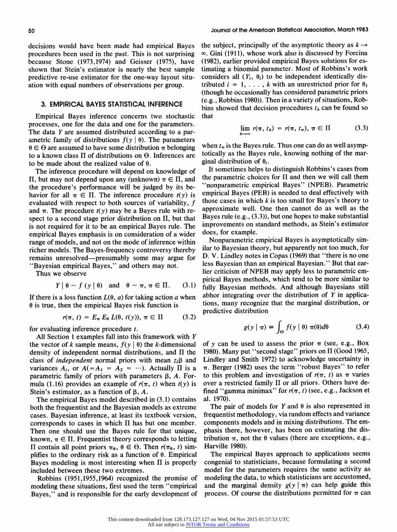
We illustrate in Figure 1 the use of empirical Bayes confidence intervals to predict the season batting averages 0i of 18 baseball players on the basis of their batting averages Yi after the first 45 at bats, that is, in the equal variance case (Efron and Morris 1975). The 45 degree line in Figure 1 is the classical estimate Yi marked "CLAS- SICAL." The shrinking rule, a modification described in Morris (1977) of Stein's estimator, has B = .675. That estimation line has a much gentler slope of 18 degrees, crossing the CLASSICAL line at Y = .266, the average of all 18 players. In this case the true averages 0i were obtained and are plotted in Figure 1. The empirical Bayes line EBE lies much nearer to the least squares regression line of 0i and Yi, because the 0i are much less variable than the Yi, and so it predicts much more accurately.

The CLASSICAL confidence bands, Yi + z VI2, also are plotted for z = 1.00 (68 percent confidence) and for z = 1.96 (95 percent confidence). They cover the right fraction of points (17 of 18 in the 95 percent case) but are quite wide because of the steep slope. The gentler slope for EBE permits shorter confidence bands, which are curved to allow for greater uncertainty at the extremes. The 95 percent empirical Bayes intervals cover all 18 points while being 37 percent shorter.

The ensemble information in this problem is strong. Thus, Y1 = .400 suggests 01 = .400 in frequentist terms, because frequency methods do not account for the fact

.500 -

c .400 - .\0/

> EBE, 975th percentile / V

:3.300//

o: EBE, 84th percentile 1 /

a) ~~~~EBE . .200 -/ /

EB E, 16th percentiler /

0/ EBE, 2.5th percentile va l

.100

CLASSICAL, Y, .000

.000 .100 .200 .300 .400

Figure 1. EIGHTEEN POINTS PLOTTED AT (Y,, 0,). CLASSICAL Yi, Y, ? Vo12, and Yt ? 1.96 V112 (dashed lines. EBE = 0i EBE

?s,, and EBE + 1.96s, (solid curves)

that all 17 other players had Y1 < .400. The PEB interval for 01, which uses this information, puts .400 at the 98th percentile, an unlikely value.

On the other hand the true value 017 = .318 is contained in the 95 percent EB interval, which is [.152, .320], but not in the frequentist confidence interval [.046, .304] for player 17. Thus the EB intervals are smaller, but are not necessarily contained in the usual intervals. In this case .318 was the true average of player 17 so only the shorter EB interval correctly covers the true value. (Player 17 was Thurman Munson, who was to become a perennial all-star.)

We could say, when reporting these intervals, "As- suming the 18 players are a random sample from a population with normally distributed batting abilities, we are 95 percent EB confident that .152 s 017 < .320." Random sampling assures the exchangeability needed for the Oi. The "EB" is included to warn the reader that this is not an ordinary confidence statement, although it might be left unmentioned because the "normally distributed batting abilities" phrase already indicates that the Oi are random. Similar statements could be made for the other 17 players.

5. EMPIRICAL BAYES CONFIDENCE INTERVALS-THE UNEQUAL VARIANCE CASE

Now consider the more general case (1.1), (1.6) when the Vi may be unequal, and all A, = A are the same. The




cases Ai = aiA with ai known, seemingly more general, can be made equivalent to the case Ai = A via transformation and relabeling.

Based on the model (1.7), (1.10), a reasonable estimate of Oi or of the posterior mean Oj* is

Oi = (1 - Bj)Yi + Bi (zi'). (5.1)

Here, with A an approximately unbiased estimate of A, i is the weighted least squares estimate

i-(Z'DZ)1-Z'DY (5.2) with D = Diag (W1, .. ., Wk), the diagonal matrix of weights

Wi -1/(Vi + A)i(53 IV,+A). (5.3) The variance A is estimated by

A E Wi{(kI(k - r)) (Yi - zi P)2 - Vi}

but we force A 2 0 if (5.4) is negative. Actually A, , must be determined by guessing atA, and then computing (5.3), (5.2), and (5.4) to improve the guess. These steps may be iterated until A converges, usually taking about four to eight cycles. Any set of weights Wi in (5.4) will make A nearly biased. The estimate (5.4) of A is not the maximum likelihood estimate of A, but is related to ones used by Fay and Herriot (1979), Carter and Rolph (1974), and "RIDGM" in Dempster, Schatzoff, and Wermuth (1977). When r = 0, the maximum likelihood estimate of A (Efron and Morris 1973) is obtained by replacing Wi with W,2 in (5.4). When r > 0 it is better to use a restricted maximum likelihood estimator (REML) of A than the MLE. The REML is given approximately by (5.4) provided Wi is replaced with W12.

Now let

Bi = ((k - r - 2)1(k - r)) Vi/(Vi + A) (5.5)

and

Si2 = Vi [1 - ((k- ri)lk) B1] + vi(Yi - zif)2. (5.6)

In (5.6) we have

ri= kWi[Z(Z'DZ) 1Z']ii (5.7)

(ri estimates the effective value of r for component i),

vi = (21(k - r - 2)) Bi2(V + A)/(Vi + A) (5.8)

(vi approximates the variance of B,), and

V = E WiVi/E Wi (5.9)

is the average variance. The interval

Oi-+ Z Si (5.10)

is proposed as an approximate empirical Bayes confidence interval containing A. with probability 1 - a = 24?(z) - 1. Evidence for this claim is incomplete, but is based on three observations.

A Y" +.420 1

t.400 / \\ 1 + 400

380

+.360

4.340 1

+ .280

+.260

I I + Year index, t

1 3 5 7 9 11 13 15 17 19 21 23

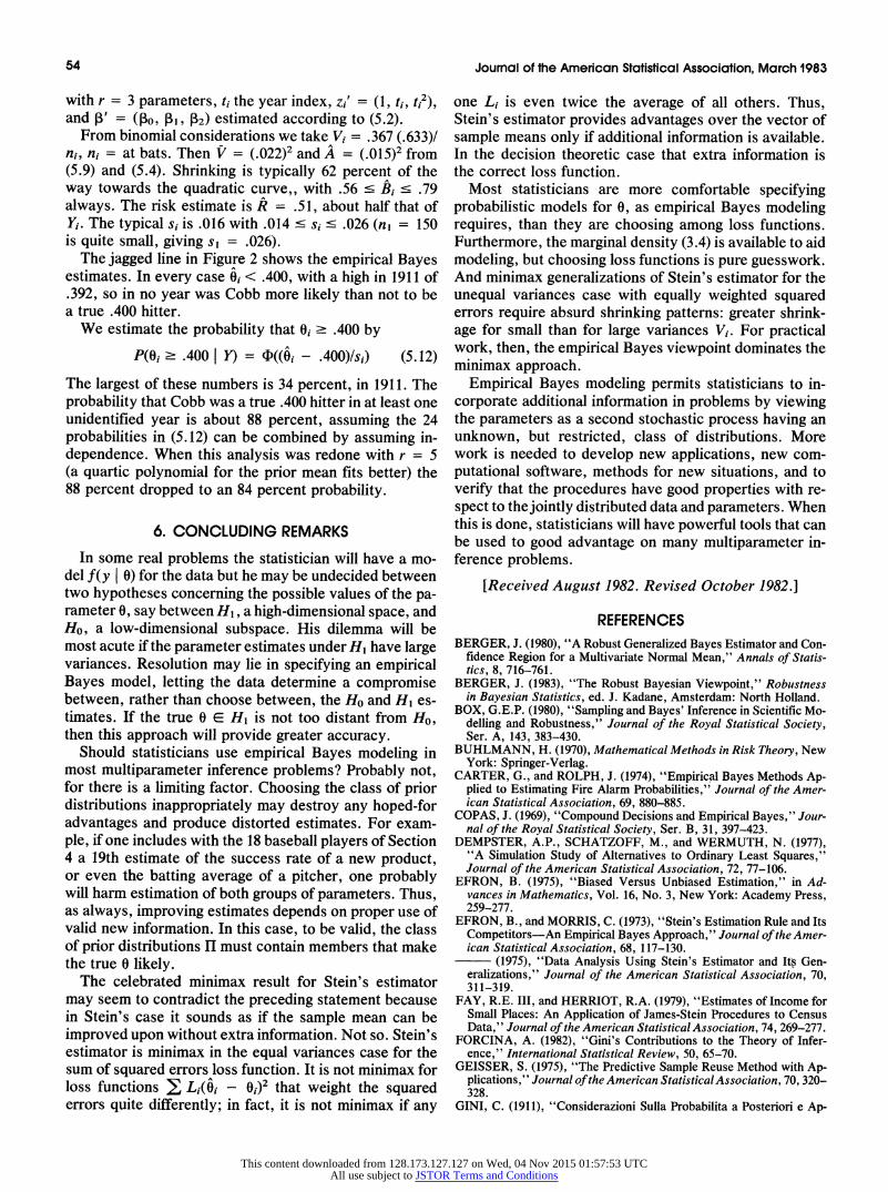
Figure 2. TY COBB'S BATTING AVERAGES, 1905-1928. 1 = ob- served average; 3 (Dark line) = regression estimator (r = 3 quadratic); 2 = empiricial Bayes estimate, shrinkages B, range from 56 to 79 percent

1. The intervals (5.10) reduce in the equal variances case to those of Section 4, which have the claimed coverage probability.

2. The proposed rule has been derived by following Bayes's theory. As k increases, A coverages to A in probability, and so Bayes's theory guarantees the correct coverage probability.

3. The coverage probabilities have held up in various computer simulations.

The unequal variance estimates and intervals just proposed will be illustrated next by a second baseball example. We ask whether Ty Cobb was ever a "true" .400 hitter for one season. Cobb had the highest lifetime batting average of all time (.367) and in 1911, 1912, and 1922 he batted over .400. Only a handful of other players ever have exceeded .400 for an entire season, no one since 1941. If there ever was a true .400 hitter, it probably was Ty Cobb. (Hornsby is the only other serious candidate.)

Figure 2 shows Cobb's batting averages Yi for the k = 24 years of his career. He batted .420 in his best year, 1911, but that is only 1.04 standard deviations above .399 for his 591 at bats. Thus we ask whether Cobb was lucky that year with Y7 > .400 but 07 < .400.

A quadratic curve fits Cobb's career performance pretty well and we take that as the prior mean

E0Z = Zi' 3o + PIt, + 32ti2 (5.11)




with r = 3 parameters, ti the year index, zi' = (1, tj, ti2), and ,B' = (Po, ,,, 12) estimated according to (5.2).

From binomial considerations we take Vi = .367 (.633)/ ni, ni = at bats. Then V = (.022)2 and A = (.015)2 from (5.9) and (5.4). Shrinking is typically 62 percent of the way towards the quadratic curve,, with .56 c Bi ' .79 always. The risk estimate is R = .51, about half that of Yi. The typical si is .016 with .014 c sic .026 (ni = 150 is quite small, giving si = .026).

The jagged line in Figure 2 shows the empirical Bayes estimates. In every case Oi < .400, with a high in 1911 of .392, so in no year was Cobb more likely than not to be a true .400 hitter.

We estimate the probability that Oi ' .400 by

P(Oi - .400 1 Y) = 1?((0i - .400)Isi) (5.12)

The largest of these numbers is 34 percent, in 1911. The probability that Cobb was a true .400 hitter in at least one unidentified year is about 88 percent, assuming the 24 probabilities in (5.12) can be combined by assuming independence. When this analysis was redone with r = 5 (a quartic polynomial for the prior mean fits better) the 88 percent dropped to an 84 percent probability.

6. CONCLUDING REMARKS In some real problems the statistician will have a mo-

del f(y 1 0) for the data but he may be undecided between two hypotheses concerning the possible values of the parameter 0, say between HI, a high-dimensional space, and Ho, a low-dimensional subspace. His dilemma will be most acute if the parameter estimates under HI have large variances. Resolution may lie in specifying an empirical Bayes model, letting the data determine a compromise between, rather than choose between, the Ho and HI estimates. If the true 8 E Hi is not too distant from Ho, then this approach will provide greater accuracy.

Should statisticians use empirical Bayes modeling in most multiparameter inference problems? Probably not, for there is a limiting factor. Choosing the class of prior distributions inappropriately may destroy any hoped-for advantages and produce distorted estimates. For example, if one includes with the 18 baseball players of Section 4 a 19th estimate of the success rate of a new product, or even the batting average of a pitcher, one probably will harm estimation of both groups of parameters. Thus, as always, improving estimates depends on proper use of valid new information. In this case, to be valid, the class of prior distributions II must contain members that make the true 0 likely.

The celebrated minimax result for Stein's estimator may seem to contradict the preceding statement because in Stein's case it sounds as if the sample mean can be improved upon without extra information. Not so. Stein's estimator is minimax in the equal variances case for the sum of squared errors loss function. It is not minimax for loss functions 2 L1(0, - 0i)2 that weight the squared errors quite differently; in fact, it is not minimax if any

one Li is even twice the average of all others. Thus, Stein's estimator provides advantages over the vector of sample means only if additional information is available. In the decision theoretic case that extra information is the correct loss function.

Most statisticians are more comfortable specifying probabilistic models for 0, as empirical Bayes modeling requires, than they are choosing among loss functions. Furthermore, the marginal density (3.4) is available to aid modeling, but choosing loss functions is pure guesswork. And minimax generalizations of Stein's estimator for the unequal variances case with equally weighted squared errors require absurd shrinking patterns: greater shrinkage for small than for large variances Vi. For practical work, then, the empirical Bayes viewpoint dominates the minimax approach.

Empirical Bayes modeling permits statisticians to in- corporate additional information in problems by viewing the parameters as a second stochastic process having an unknown, but restricted, class of distributions. More work is needed to develop new applications, new com- putational software, methods for new situations, and to verify that the procedures have good properties with respect to the jointly distributed data and parameters. When this is done, statisticians will have powerful tools that can be used to good advantage on many multiparameter inference problems.

[Received August 1982. Revised October 1982.]

REFERENCES BERGER, J. (1980), "A Robust Generalized Bayes Estimator and Con-

fidence Region for a Multivariate Normal Mean," Annals of Statis- tics, 8, 716-761.

BERGER, J. (1983), "The Robust Bayesian Viewpoint," Robustness in Bayesian Statistics, ed. J. Kadane, Amsterdam: North Holland.

BOX, G.E.P. (1980), "Sampling and Bayes' Inference in Scientific Mo- delling and Robustness," Journal of the Royal Statistical Society, Ser. A, 143, 383-430.

BUHLMANN, H. (1970), Mathematical Methods in Risk Theory, New York: Springer-Verlag.

CARTER, G., and ROLPH, J. (1974), '"Empirical Bayes Methods Ap- plied to Estimating Fire Alarm Probabilities," Journal of the Amer- ican Statistical Association, 69, 880-885.

COPAS, J. (1969), "Compound Decisions and Empirical Bayes," Jour- nal of the Royal Statistical Society, Ser. B, 31, 397-423.

DEMPSTER, A.P., SCHATZOFF, M., and WERMUTH, N. (1977), "A Simulation Study of Alternatives to Ordinary Least Squares," Journal of the American Statistical Association, 72, 77-106.

EFRON, B. (1975), "Biased Versus Unbiased Estimation," in Ad- vances in Mathematics, Vol. 16, No. 3, New York: Academy Press, 259-277.

EFRON, B., and MORRIS, C. (1973), "Stein's Estimation Rule and Its Competitors-An Empirical Bayes Approach," Journal of the Amer- ican Statistical Association, 68, 117-130.

(1975), "Data Analysis Using Stein's Estimator and Its Gen- eralizations," Journal of the American Statistical Association, 70, 311-319.

FAY, R.E. III, and HERRIOT, R.A. (1979), "Estimates of Income for Small Places: An Application of James-Stein Procedures to Census Data," Journal of the American Statistical Association, 74, 269-277.

FORCINA, A. (1982), "Gini's Contributions to the Theory of Infer- ence," International Statistical Review, 50, 65-70.

GEISSER, S. (1975), "The Predictive Sample Reuse Method with Ap- plications, " Journal of the American Statistical Association, 70, 320- 328.

GINI, C. (1911), "Considerazioni Sulla Probabilita a Posteriori e Ap-



Berger: Comment on Parametric Empirical Bayes Inference 55

plicazioni al Rapporto dei Sessi Nelle Nascite Umane," Metron, 15, 133-172.

GOOD, I.J. (1965), The Estimation of Probabilities: An Essay on Mod- ern Bayesian Methods, Cambridge: Massachusetts Institute of Tech- nology Press.

HARVILLE, D. (1980), "Predictions for National Football League Games via Linear-Model Methodology," Journal of the American Statistical Association, 75, 516-524.

HOADLEY, B. (1981), "Quality Management Plan (QMP)," Bell Sys- tem Technical Journal, 60, 215-273.

JACKSON, D.A., DONOVAN, T.M., ZIMMER, W.J., and DEELEY, J.J. (1970), "r2-Minimax Estimators in the Exponential Family," Biometrika, 57, 439-443.

JAMES, W., and STEIN, C. (1961), "Estimation with Quadratic Loss," Proceedings of the Fourth Berkeley Sumposium on Mathematical Statistics and Probability (Vol. 1), University of California Press, Berkeley, 361-379.

LINDLEY, D.V., and SMITH, A.F.M. (1972), "Bayes Estimates for the Linear Model," Journal of the Royal Statistical Society, Ser. B, 34, 1-41.

MORRIS, C. (1977), "Interval Estimation for Empirical Bayes Gen- eralizations of Stein's Estimator," Proceedings of the Twenty-Second Conference on the Design of Experiments in Army Research Devel- opment and Testing, ARO Report 77-2.

(1981), "Parametric Empirical Bayes Confidence Intervals," to appear in the Proceedings of the Conference on Scientific Inference, Data Analysis and Robustness, University of Wisconsin.

(1982), "Natural Exponential Families With Quadratic Variance Functions," The Annals of Statistics, 10, 65-80.

(1983), "Natural Exponential Families With Quadratic Variance Functions: Statistical Theory," The Annals of Statistics, 11.

MORRIS, C., and VAN SLYKE, L. (1978), "Empirical Bayes Methods for Pricing Insurance Classes," Proceedings of the Business and Eco- nomics Statistics Section, American Statistical Association, 579-582.

ROBBINS, H. (1951), "Asymptotically Subminimax Solutions of Com- pound Statistical Decision Problems," Proceedings of the Second Berkeley Symposium on Mathematics, Statistics and Probability, University of California Press, 131-148.

(1955), "An Empirical Bayes Approach to Statistics," Pro- ceedings of the ThirdBerkeley Symposium on Mathematics, Statistics and Probability, Vol. 1, 157-164.

(1964), "The Empirical Bayes Approach to Statistical Decision Problems," The Annals of Mathematical Statistics, 35, 1-20.

(1980), "An Empirical Bayes Estimation Problem," Proceedings of the National Academy of Sciences USA, 77, 12, 6988-6989.

RUBIN, D. (1981), "Using Empirical Bayes Techniques in the Law School Validity Studies," Journal of the American Statistical As- sociation, 75, 801-827, with discussion.

STONE, M. (1973), "Discussion of the Paper by Professor Efron and Dr. Morris," Journal of the Royal Statistical Society, Ser. B, 35, 408- 409.

(1974), "Cross-validatory Choice and Assessment of Statistical Predictions" (with discussion), Journal of the Royal Statistical Soci- ety, Ser. B, 36, 111-147.

VAN DER MERWE, A.J., GROENEWALD, P.C.N., NEL, D.G., and VAN DER MERWE, C.A. (1981), "Confidence Intervals for a Multi- variate Normal Mean in the Case of Empirical Bayes Estimation Using Pearson Curves and Normal Approximations," Tech. Rept. No. 70, Department of Mathematics and Statistics, University of The Orange Free State, Bloemfontein, South Africa, November.

WHITNEY, A.W. (1918), "The Theory of Experience Rating," Pro- ceedings of the Casualty Actuarial Society, Vol. IV, 274-292.

omment JAMES BERGER*

Morris has provided us with an excellent description of parametric empirical Bayes inference as it applies to estimation of normal means. The techniques he reviews (many developed by himself) seem eminently sound and useful for the types of problems he considers. My com- ments will address (a) applicability, (b) Bayesian aspects, (c) minimax aspects, and (d) robustness of the theory.

1. APPLICABILITY OF PARAMETRIC EMPIRICAL BAYES THEORY

For the small to moderately large dimensional problems most frequently encountered, I agree with Morris that it is necessary to postulate a model for the unknown means Oi and estimate the parameters for this model, rather than try nonparametric estimation of the (assumed) common prior. There are rarely enough data for the nonparametric approach to prove successful, and a rather large degree of robustness with respect to the postulated model is present, as will be mentioned later.

* James Berger is Professor of Statistics, Department of Statistics, Purdue University, West Lafayette, IN 47907. Research was supported by the National Science Foundation, Grant MCS 81-01670A1.

It is also worth emphasizing Morris's comment that the parametric empirical Bayes approach is generally very worthwhile when one is trying to decide between a higher or lower dimensional model for the parameters of inter- est. A relatively common instance of this is when one is trying to decide whether to use a pooled estimate of variance or individual estimates. It can rarely be correct, when doubt exists, to use one extreme or the other; an empirical Bayes compromise is typically much better.

The development of empirical Bayes confidence sets is very important, not just as a necessary adjunct to estimation but also since tests can be done using the confidence sets. A related important aspect of the theory is its effect on "ranking problems." In the unequal variance case the empirical Bayes estimates will often be ordered differently from the original estimates Yi, essentially because an "extreme" Yi with large variance will be shrunk a substantial amount towards the estimated prior mean, perhaps leapfrogging a Yi with a smaller variance. The resulting ordering of the population means is usually much more accurate and can allow substantially better selection of "extreme" Oi.

It should be mentioned that the theory does not demand that simultaneous estimation of all Oi be applicable. For



Documents

Parametric Empirical Bayes Inference: Theory and ... & Francis, Ltd. and American Statistical Association are collaborating with JSTOR to digitize, preserve and extend access to Journal