PARAMETRIC EQUATIONS AND POLAR COORDINATES · 2017-11-17 · CURVES DEFINED BY PARAMETRIC EQUATIONS Imagine that a particle moves along the curve shown in Figure 1. It is impossible

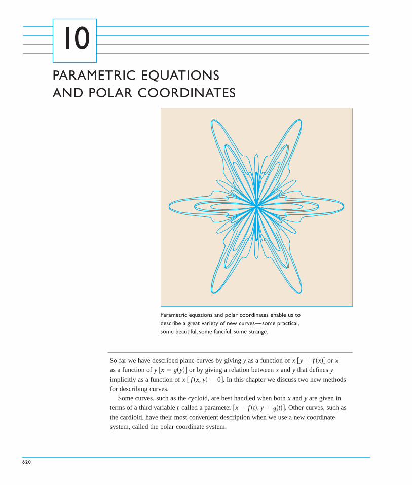
620

So far we have described plane curves by giving as a function of or

as a function of or by giving a relation between and that defines

implicitly as a function of . In this chapter we discuss two new methods

for describing curves.

Some curves, such as the cycloid, are best handled when both and are given in

terms of a third variable called a parameter . Other curves, such as

the cardioid, have their most convenient description when we use a new coordinate

system, called the polar coordinate system.

�x � f �t�, y � t�t��t

yx

� f �x, y� � 0�x

yyx�x � t�y��y

x�y � f �x��xy

Parametric equations and polar coordinates enable us todescribe a great variety of new curves—some practical,some beautiful, some fanciful, some strange.

PARAMETRIC EQUATIONS AND POLAR COORDINATES

10

CURVES DEFINED BY PARAMETRIC EQUATIONS

Imagine that a particle moves along the curve C shown in Figure 1. It is impossible todescribe C by an equation of the form because C fails the Vertical Line Test. Butthe x- and y-coordinates of the particle are functions of time and so we can write and . Such a pair of equations is often a convenient way of describing a curve andgives rise to the following definition.

Suppose that and are both given as functions of a third variable (called a param-eter) by the equations

(called parametric equations). Each value of determines a point , which we canplot in a coordinate plane. As varies, the point varies and traces outa curve , which we call a parametric curve. The parameter t does not necessarily repre-sent time and, in fact, we could use a letter other than t for the parameter. But in manyapplications of parametric curves, t does denote time and therefore we can interpret

as the position of a particle at time t.

EXAMPLE 1 Sketch and identify the curve defined by the parametric equations

SOLUTION Each value of gives a point on the curve, as shown in the table. For instance, if, then , and so the corresponding point is . In Figure 2 we plot the

points determined by several values of the parameter and we join them to producea curve.

A particle whose position is given by the parametric equations moves along the curvein the direction of the arrows as increases. Notice that the consecutive points marked onthe curve appear at equal time intervals but not at equal distances. That is because theparticle slows down and then speeds up as increases.

It appears from Figure 2 that the curve traced out by the particle may be a parabola.This can be confirmed by eliminating the parameter as follows. We obtain from the second equation and substitute into the first equation. This gives

and so the curve represented by the given parametric equations is the parabola. Mx � y 2 � 4y � 3

x � t 2 � 2t � �y � 1�2 � 2�y � 1� � y 2 � 4y � 3

t � y � 1t

t

t

FIGURE 2

0

t=0

t=1

t=2

t=3

t=4

t=_1

t=_2

(0, 1)

y

x

8

�x, y��0, 1�y � 1x � 0t � 0

t

y � t � 1x � t2 � 2t

�x, y� � � f �t�, t�t��

C�x, y� � � f �t�, t�t��t

�x, y�t

y � t�t�x � f �t�

tyx

y � t�t�x � f �t�

y � f �x�

10.1

t x y

�2 8 �1�1 3 0

0 0 11 �1 22 0 33 3 44 8 5

N This equation in and describes where theparticle has been, but it doesn’t tell us when theparticle was at a particular point. The parametricequations have an advantage––they tell uswhen the particle was at a point. They also indi-cate the direction of the motion.

yx

C

0

(x, y)={f(t), g(t)}

FIGURE 1

y

x

621

No restriction was placed on the parameter in Example 1, so we assumed that t couldbe any real number. But sometimes we restrict t to lie in a finite interval. For instance, theparametric curve

shown in Figure 3 is the part of the parabola in Example 1 that starts at the point andends at the point . The arrowhead indicates the direction in which the curve is tracedas increases from 0 to 4.

In general, the curve with parametric equations

has initial point and terminal point .

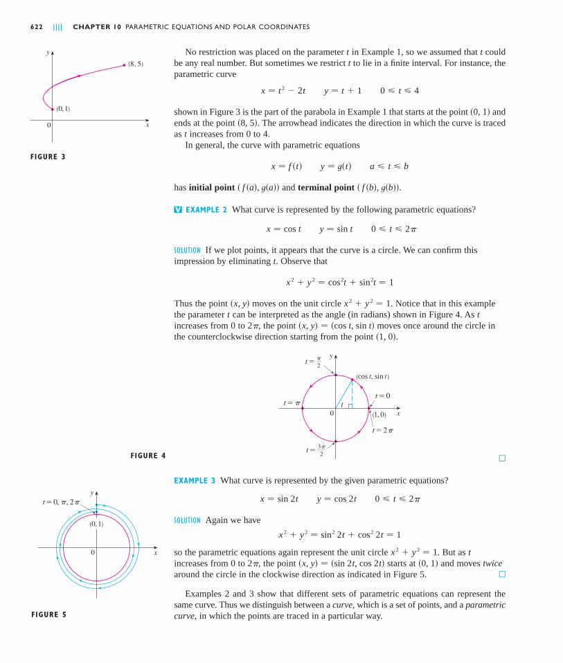
EXAMPLE 2 What curve is represented by the following parametric equations?

SOLUTION If we plot points, it appears that the curve is a circle. We can confirm thisimpression by eliminating Observe that

Thus the point moves on the unit circle . Notice that in this examplethe parameter can be interpreted as the angle (in radians) shown in Figure 4. As increases from 0 to , the point moves once around the circle inthe counterclockwise direction starting from the point .

M

EXAMPLE 3 What curve is represented by the given parametric equations?

SOLUTION Again we have

so the parametric equations again represent the unit circle . But as increases from 0 to , the point starts at and moves twicearound the circle in the clockwise direction as indicated in Figure 5. M

Examples 2 and 3 show that different sets of parametric equations can represent thesame curve. Thus we distinguish between a curve, which is a set of points, and a parametriccurve, in which the points are traced in a particular way.

�0, 1��x, y� � �sin 2t, cos 2t�2�tx 2 � y 2 � 1

x 2 � y 2 � sin2 2t � cos2 2t � 1

0 � t � 2�y � cos 2tx � sin 2t

FIGURE 4 3π

2t=

π

2t=

0

tt=0

(1, 0)

(cos t, sin t )

t=2π

t=π

x

y

�1, 0��x, y� � �cos t, sin t�2�

ttx 2 � y 2 � 1�x, y�

x 2 � y 2 � cos2t � sin2t � 1

t.

0 � t � 2�y � sin tx � cos t

V

� f �b�, t�b�� f �a�, t�a��

a � t � by � t�t�x � f �t�

t�8, 5�

�0, 1�

0 � t � 4y � t � 1x � t 2 � 2t

t

622 | | | | CHAPTER 10 PARAMETRIC EQUATIONS AND POLAR COORDINATES

FIGURE 3

0

(8, 5)

(0, 1)

y

x

0

t=0, π, 2π

FIGURE 5

x

y

(0, 1)

EXAMPLE 4 Find parametric equations for the circle with center and radius .

SOLUTION If we take the equations of the unit circle in Example 2 and multiply the expres-sions for and by , we get , . You can verify that these equationsrepresent a circle with radius and center the origin traced counterclockwise. We nowshift units in the -direction and units in the -direction and obtain parametric equa-tions of the circle (Figure 6) with center and radius :

M

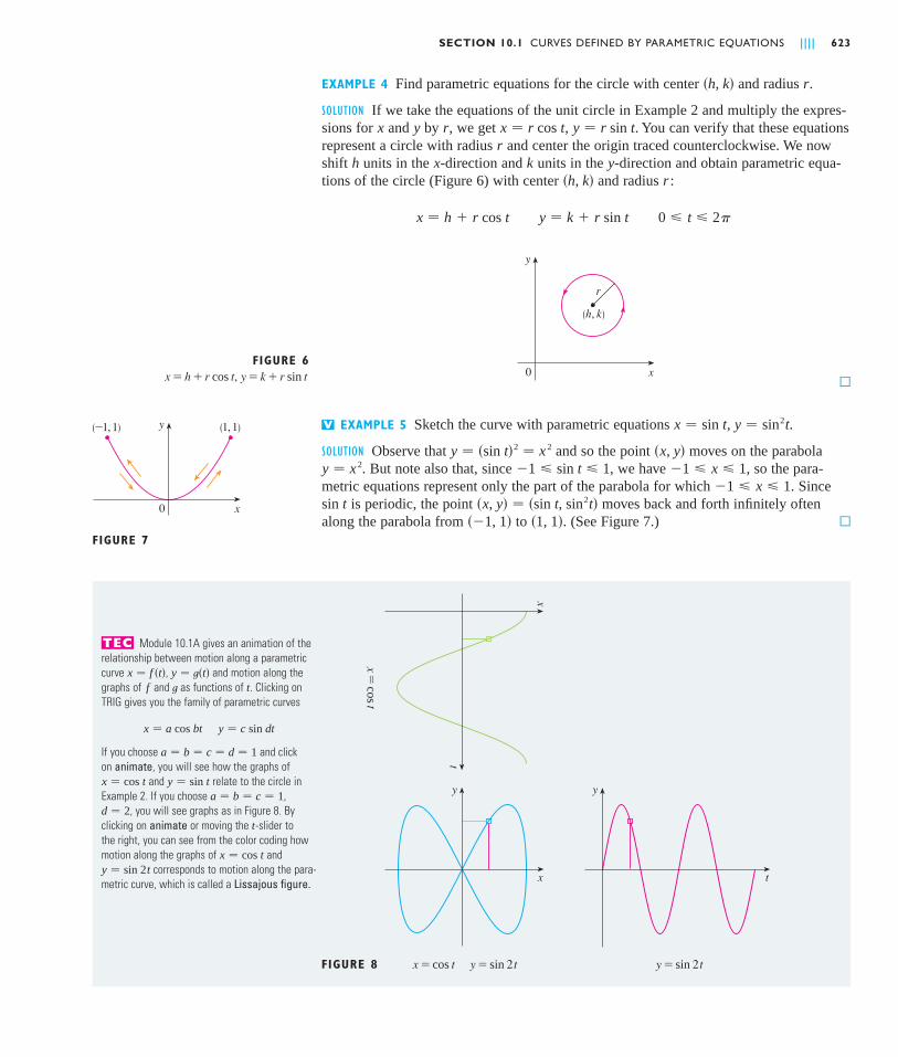
EXAMPLE 5 Sketch the curve with parametric equations , .

SOLUTION Observe that and so the point moves on the parabola. But note also that, since , we have , so the para-

metric equations represent only the part of the parabola for which . Sinceis periodic, the point moves back and forth infinitely often

along the parabola from to . (See Figure 7.) M

y=sin 2tx=cos t y=sin 2t

x=

cos t

FIGURE 8

t

x

y

t

y

x

�1, 1��1, 1��x, y� � �sin t, sin2t�sin t

�1 � x � 1�1 � x � 1�1 � sin t � 1y � x 2

�x, y�y � �sin t�2 � x 2

y � sin2tx � sin tV

FIGURE 6x=h+r cos t, y=k+r sin t 0

(h, k)

r

x

y

0 � t � 2�y � k � r sin tx � h � r cos t

r�h, k�ykxh

ry � r sin tx � r cos tryx

r�h, k�

SECTION 10.1 CURVES DEFINED BY PARAMETRIC EQUATIONS | | | | 623

Module 10.1A gives an animation of therelationship between motion along a parametriccurve , and motion along thegraphs of and as functions of . Clicking onTRIG gives you the family of parametric curves

If you choose and click on animate, you will see how the graphs of

and relate to the circle inExample 2. If you choose ,

, you will see graphs as in Figure 8. Byclicking on animate or moving the -slider to the right, you can see from the color coding howmotion along the graphs of and

corresponds to motion along the para-metric curve, which is called a Lissajous figure.y � sin 2t

x � cos t

td � 2

a � b � c � 1y � sin tx � cos t

a � b � c � d � 1

y � c sin dtx � a cos bt

ttfy � t�t�x � f �t�

TEC

FIGURE 7

0

(1, 1)(_1, 1)

x

y

GRAPHING DEVICES

Most graphing calculators and computer graphing programs can be used to graph curvesdefined by parametric equations. In fact, it’s instructive to watch a parametric curve beingdrawn by a graphing calculator because the points are plotted in order as the correspon-ding parameter values increase.

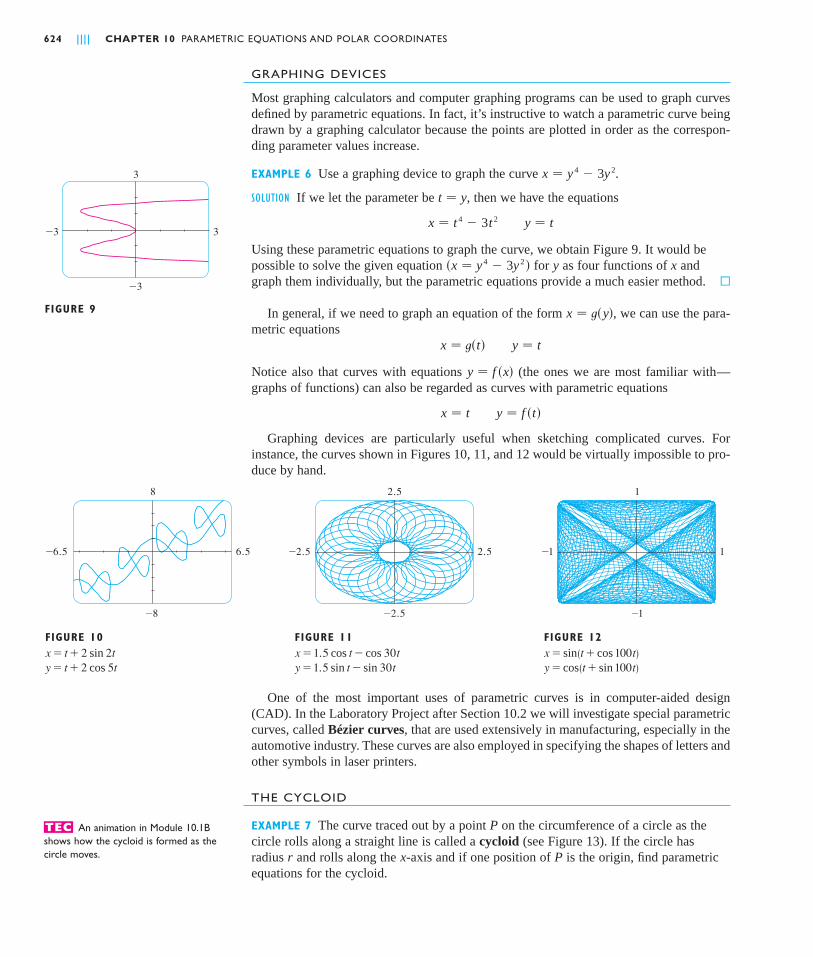
EXAMPLE 6 Use a graphing device to graph the curve .

SOLUTION If we let the parameter be , then we have the equations

Using these parametric equations to graph the curve, we obtain Figure 9. It would bepossible to solve the given equation for y as four functions of x andgraph them individually, but the parametric equations provide a much easier method. M

In general, if we need to graph an equation of the form , we can use the para-metric equations

Notice also that curves with equations (the ones we are most familiar with—graphs of functions) can also be regarded as curves with parametric equations

Graphing devices are particularly useful when sketching complicated curves. For instance, the curves shown in Figures 10, 11, and 12 would be virtually impossible to pro-duce by hand.

One of the most important uses of parametric curves is in computer-aided design(CAD). In the Laboratory Project after Section 10.2 we will investigate special parametriccurves, called Bézier curves, that are used extensively in manufacturing, especially in theautomotive industry. These curves are also employed in specifying the shapes of letters andother symbols in laser printers.

THE CYCLOID

EXAMPLE 7 The curve traced out by a point on the circumference of a circle as thecircle rolls along a straight line is called a cycloid (see Figure 13). If the circle hasradius and rolls along the -axis and if one position of is the origin, find parametricequations for the cycloid.

Pxr

P

8

_8

_6.5 6.5

FIGURE 10x=t+2 sin 2t

y=t+2 cos 5t

2.5

_2.5

2.5

FIGURE 11x=1.5 cos t-cos 30t

y=1.5 sin t-sin 30t

_2.5

1

_1

1

FIGURE 12x=sin(t+cos 100t)

y=cos(t+sin 100t)

_1

y � f �t�x � t

y � f �x�

y � tx � t�t�

x � t�y�

�x � y 4 � 3y 2 �

y � tx � t 4 � 3t 2

t � y

x � y 4 � 3y 2


An animation in Module 10.1Bshows how the cycloid is formed as thecircle moves.

TEC

3

_3

_3 3

FIGURE 9

SOLUTION We choose as parameter the angle of rotation of the circle when is atthe origin). Suppose the circle has rotated through radians. Because the circle has beenin contact with the line, we see from Figure 14 that the distance it has rolled from theorigin is

Therefore the center of the circle is . Let the coordinates of be . Thenfrom Figure 14 we see that

Therefore parametric equations of the cycloid are

One arch of the cycloid comes from one rotation of the circle and so is described by. Although Equations 1 were derived from Figure 14, which illustrates the

case where , it can be seen that these equations are still valid for othervalues of (see Exercise 39).

Although it is possible to eliminate the parameter from Equations 1, the resultingCartesian equation in and is very complicated and not as convenient to work with asthe parametric equations. M

One of the first people to study the cycloid was Galileo, who proposed that bridges bebuilt in the shape of cycloids and who tried to find the area under one arch of a cycloid.Later this curve arose in connection with the brachistochrone problem: Find the curvealong which a particle will slide in the shortest time (under the influence of gravity) froma point to a lower point not directly beneath . The Swiss mathematician JohnBernoulli, who posed this problem in 1696, showed that among all possible curves thatjoin to , as in Figure 15, the particle will take the least time sliding from to if thecurve is part of an inverted arch of a cycloid.

The Dutch physicist Huygens had already shown that the cycloid is also the solution tothe tautochrone problem; that is, no matter where a particle is placed on an invertedcycloid, it takes the same time to slide to the bottom (see Figure 16). Huygens proposedthat pendulum clocks (which he invented) swing in cycloidal arcs because then the pendu-lum takes the same time to make a complete oscillation whether it swings through a wideor a small arc.

FAMILIES OF PARAMETRIC CURVES

EXAMPLE 8 Investigate the family of curves with parametric equations

What do these curves have in common? How does the shape change as increases?a

y � a tan t � sin tx � a � cos t

V

P

BABA

ABA

yx�

�0 � � � ��2

0 � � � 2�

� � �y � r �1 � cos ��x � r �� sin ��1

y � � TC � � � QC � � r � r cos � � r �1 � cos ��

x � � OT � � � PQ � � r� � r sin � � r�� sin ��

�x, y�PC�r�, r�

� OT � � arc PT � r�

�P�� 0�

FIGURE 13 P

P

P


FIGURE 15

A

B

cycloid

FIGURE 14

xO

y

T

C(r¨, r )r ¨

xy

r¨

P Q

P

PP

P

P

FIGURE 16

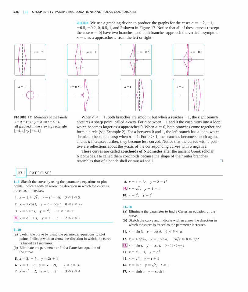
SOLUTION We use a graphing device to produce the graphs for the cases , ,, , , , , and shown in Figure 17. Notice that all of these curves (except

the case ) have two branches, and both branches approach the vertical asymptoteas approaches from the left or right.

When , both branches are smooth; but when reaches , the right branchacquires a sharp point, called a cusp. For between and 0 the cusp turns into a loop,which becomes larger as approaches 0. When , both branches come together andform a circle (see Example 2). For between 0 and 1, the left branch has a loop, whichshrinks to become a cusp when . For , the branches become smooth again,and as increases further, they become less curved. Notice that the curves with posi-tive are reflections about the -axis of the corresponding curves with negative.

These curves are called conchoids of Nicomedes after the ancient Greek scholarNicomedes. He called them conchoids because the shape of their outer branches resembles that of a conch shell or mussel shell. M

ayaa

a � 1a � 1a

a � 0a�1a

�1aa � �1

a=_2 a=_1 a=_0.5 a=_0.2

a=2a=1a=0.5a=0

axx � aa � 0

210.50�0.2�0.5�1a � �2

8. ,

,

10. ,

11–18(a) Eliminate the parameter to find a Cartesian equation of the

curve.(b) Sketch the curve and indicate with an arrow the direction in

which the curve is traced as the parameter increases.

11. , ,

12. , ,

, ,

14. ,

15. ,

16. , ,

17. , y � cosh tx � sinh t

t 1y � st x � ln t

y � t � 1x � e 2t

y � e 2tx � et � 1

0 � t � ��2y � csc tx � sin t13.

��2 � � � ��2y � 5 sin �x � 4 cos �

0 � � � �y � cos �x � sin �

y � t 3x � t 2

y � 1 � tx � st 9.

y � 2 � t 2x � 1 � 3t1–4 Sketch the curve by using the parametric equations to plotpoints. Indicate with an arrow the direction in which the curve istraced as increases.

1. , ,

2. , ,

3. , ,

, ,

5–10(a) Sketch the curve by using the parametric equations to plot

points. Indicate with an arrow the direction in which the curveis traced as t increases.

(b) Eliminate the parameter to find a Cartesian equation of the curve.

5. ,

6. , ,

7. , , �3 � t � 4y � 5 � 2tx � t 2 � 2

�2 � t � 3y � 5 � 2tx � 1 � t

y � 2t � 1x � 3t � 5

�2 � t � 2y � e t � tx � e�t � t4.

�� t � �y � t 2x � 5 sin t

0 � t � 2�y � t � cos tx � 2 cos t

0 � t � 5y � t 2 � 4 tx � 1 � st

t

EXERCISES10.1


FIGURE 17 Members of the familyx=a+cos t, y=a tan t+sin t,

all graphed in the viewing rectangle�_4, 4� by �_4, 4�

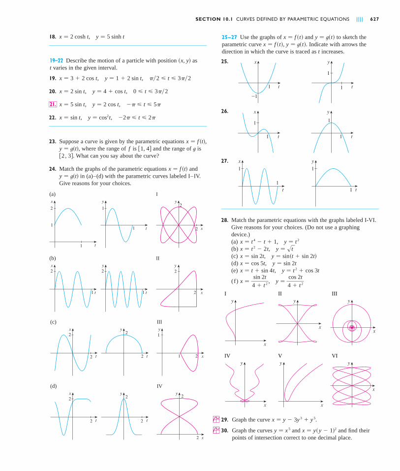
25–27 Use the graphs of and to sketch theparametric curve , . Indicate with arrows thedirection in which the curve is traced as increases.

25.

26.

27.

28. Match the parametric equations with the graphs labeled I-VI.Give reasons for your choices. (Do not use a graphingdevice.)(a) ,(b) ,(c) ,(d) ,(e) ,

(f) ,

; 29. Graph the curve .

; 30. Graph the curves and and find theirpoints of intersection correct to one decimal place.

x � y�y � 1�2y � x 5

x � y � 3y 3 � y 5

x

y

x

y

x

y

x

y

x

y

x

y

I II III

IV V VI

y �cos 2t

4 � t 2x �sin 2t

4 � t 2

y � t 2 � cos 3tx � t � sin 4ty � sin 2tx � cos 5ty � sin�t � sin 2t�x � sin 2t

y � st x � t 2 � 2ty � t 2x � t 4 � t � 1

t

y

1

1t

x

1

1

t

x

1

1 t

y

1

1

t

x

_1

1 t

y

1

1

ty � t�t�x � f �t�

y � t�t�x � f �t�18. ,

19–22 Describe the motion of a particle with position as varies in the given interval.

19. , ,

20. , ,

, ,

22. , ,

23. Suppose a curve is given by the parametric equations ,, where the range of is and the range of is

. What can you say about the curve?

24. Match the graphs of the parametric equations andin (a)–(d) with the parametric curves labeled I–IV.

Give reasons for your choices.

(c) III

t

2

2

yx

t

2

2

(d) IV

t

2

2

yx

t

2

2

y

x

2

2

1

y

x

1

2

t

x

2

1

1

t

y

1

1

y

x

2

2

(a) I

(b) IIx

t

2

1 t

2

1

y y

x

2

2

y � t�t�x � f �t�

�2, 3�t�1, 4�fy � t�t�

x � f �t�

�2� � t � 2�y � cos2tx � sin t

�� t � 5�y � 2 cos tx � 5 sin t21.

0 � t � 3��2y � 4 � cos tx � 2 sin t

��2 � t � 3��2y � 1 � 2 sin tx � 3 � 2 cos t

t�x, y�

y � 5 sinh tx � 2 cosh t


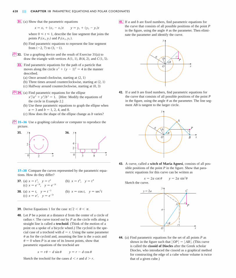
If and are fixed numbers, find parametric equations forthe curve that consists of all possible positions of the point in the figure, using the angle as the parameter. Then elimi-nate the parameter and identify the curve.

42. If and are fixed numbers, find parametric equations forthe curve that consists of all possible positions of the point in the figure, using the angle as the parameter. The line seg-ment is tangent to the larger circle.

43. A curve, called a witch of Maria Agnesi, consists of all pos-sible positions of the point in the figure. Show that para-metric equations for this curve can be written as

Sketch the curve.

44. (a) Find parametric equations for the set of all points asshown in the figure such that . (This curveis called the cissoid of Diocles after the Greek scholarDiocles, who introduced the cissoid as a graphical methodfor constructing the edge of a cube whose volume is twicethat of a given cube.)

� OP � � � AB �P

O x

a

A P

y=2a

¨

yC

y � 2a sin2�x � 2a cot �

P

O x

y

¨

ab

A

B

P

AB�

Pba

O

y

x

¨

ab P

�P

ba41.(a) Show that the parametric equations

where , describe the line segment that joins thepoints and .

(b) Find parametric equations to represent the line segmentfrom to .

; 32. Use a graphing device and the result of Exercise 31(a) todraw the triangle with vertices , , and .

Find parametric equations for the path of a particle thatmoves along the circle in the mannerdescribed.(a) Once around clockwise, starting at (b) Three times around counterclockwise, starting at (c) Halfway around counterclockwise, starting at

; (a) Find parametric equations for the ellipse. [Hint: Modify the equations of

the circle in Example 2.](b) Use these parametric equations to graph the ellipse when

and b � 1, 2, 4, and 8.(c) How does the shape of the ellipse change as b varies?

; 35–36 Use a graphing calculator or computer to reproduce thepicture.

35. 36.

37–38 Compare the curves represented by the parametric equa-tions. How do they differ?

37. (a) , (b) ,(c) ,

38. (a) , (b) ,(c) ,

39. Derive Equations 1 for the case .

40. Let be a point at a distance from the center of a circle ofradius . The curve traced out by as the circle rolls along astraight line is called a trochoid. (Think of the motion of apoint on a spoke of a bicycle wheel.) The cycloid is the spe-cial case of a trochoid with . Using the same parameter

as for the cycloid and, assuming the line is the -axis andwhen is at one of its lowest points, show that

parametric equations of the trochoid are

Sketch the trochoid for the cases and .d � rd � r

y � r � d cos � x � r� � d sin �

P� � 0x�

d � r

PrdP

��2 � � � �

y � e�2tx � e ty � sec2tx � cos ty � t �2x � t

y � e�2tx � e�3ty � t 4x � t 6y � t 2x � t 3

0

y

x

2

3 8

4

0

2

y

x2

a � 3

x 2�a 2 � y 2�b 2 � 134.

�0, 3��2, 1�

�2, 1�

x 2 � �y � 1�2 � 433.

C �1, 5�B �4, 2�A �1, 1�

�3, �1��2, 7�

P2�x 2, y2 �P1�x1, y1�0 � t � 1

y � y1 � �y2 � y1�tx � x1 � �x 2 � x1�t

31.


LABORATORY PROJECT RUNNING CIRCLES AROUND CIRCLES | | | | 629

given by the parametric equations

where is the acceleration due to gravity ( m�s ).(a) If a gun is fired with and m�s, when

will the bullet hit the ground? How far from the gun willit hit the ground? What is the maximum height reached by the bullet?

; (b) Use a graphing device to check your answers to part (a).Then graph the path of the projectile for several other values of the angle to see where it hits the ground.Summarize your findings.

(c) Show that the path is parabolic by eliminating the parameter.

; Investigate the family of curves defined by the parametricequations , . How does the shape change as increases? Illustrate by graphing several members of thefamily.

; 48. The swallowtail catastrophe curves are defined by the para-metric equations , . Graph several of these curves. What features do the curves have in common? How do they change when increases?

; The curves with equations , arecalled Lissajous figures. Investigate how these curves varywhen , , and vary. (Take to be a positive integer.)

; 50. Investigate the family of curves defined by the parametricequations , , where . Start by letting be a positive integer and see what happens to theshape as increases. Then explore some of the possibilitiesthat occur when is a fraction.c

cc

c � 0y � sin t � sin ctx � cos t

nnba

y � b cos tx � a sin nt49.

c

y � �ct 2 � 3t 4x � 2ct � 4t 3

cy � t 3 � ctx � t 2

47.

v0 � 500 � 30�

29.8t

y � �v0 sin �t �12 tt 2x � �v0 cos �t

(b) Use the geometric description of the curve to draw arough sketch of the curve by hand. Check your work byusing the parametric equations to graph the curve.

; 45. Suppose that the position of one particle at time is given by

and the position of a second particle is given by

(a) Graph the paths of both particles. How many points ofintersection are there?

(b) Are any of these points of intersection collision points? In other words, are the particles ever at the same place atthe same time? If so, find the collision points.

(c) Describe what happens if the path of the second particleis given by

46. If a projectile is fired with an initial velocity of meters persecond at an angle above the horizontal and air resistanceis assumed to be negligible, then its position after seconds is t

v0

x 2 � 3 � cos t y2 � 1 � sin t 0 � t � 2�

0 � t � 2�y2 � 1 � sin tx 2 � �3 � cos t

0 � t � 2�y1 � 2 cos tx1 � 3 sin t

t

xO

y

A

Px=2a

B

a

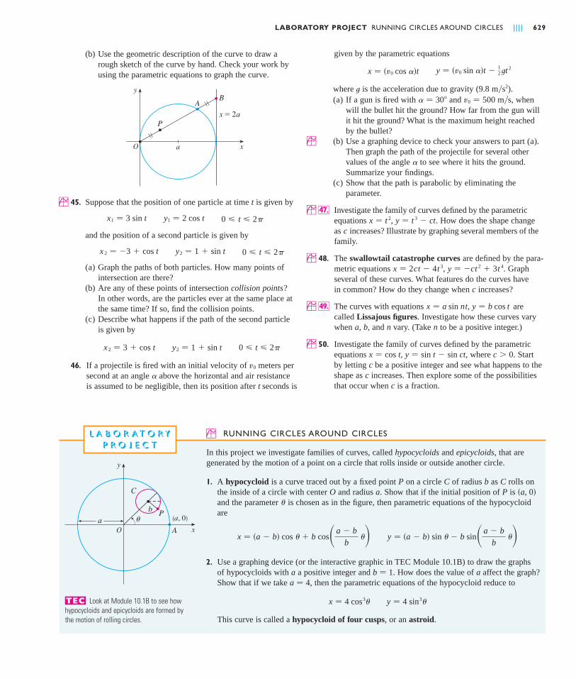
In this project we investigate families of curves, called hypocycloids and epicycloids, that aregenerated by the motion of a point on a circle that rolls inside or outside another circle.

1. A hypocycloid is a curve traced out by a fixed point P on a circle C of radius b as C rolls onthe inside of a circle with center O and radius a. Show that if the initial position of P is and the parameter is chosen as in the figure, then parametric equations of the hypocycloidare

2. Use a graphing device (or the interactive graphic in TEC Module 10.1B) to draw the graphsof hypocycloids with a a positive integer and b � 1. How does the value of a affect the graph?Show that if we take a � 4, then the parametric equations of the hypocycloid reduce to

This curve is called a hypocycloid of four cusps, or an astroid.

y � 4 sin3�x � 4 cos3�

y � �a � b� sin � � b sin�a � b

b �x � �a � b� cos � � b cos�a � b

b �

��a, 0�

; RUNNING CIRCLES AROUND CIRCLESL A B O R AT O R YP R O J E C T

xO

y

a

C

Pb

(a, 0)¨

A

Look at Module 10.1B to see howhypocycloids and epicycloids are formed by the motion of rolling circles.

TEC


3. Now try b � 1 and , a fraction where n and d have no common factor. First let n � 1and try to determine graphically the effect of the denominator d on the shape of the graph.Then let n vary while keeping d constant. What happens when ?

4. What happens if and is irrational? Experiment with an irrational number like or . Take larger and larger values for and speculate on what would happen if we

were to graph the hypocycloid for all real values of .

5. If the circle rolls on the outside of the fixed circle, the curve traced out by is called anepicycloid. Find parametric equations for the epicycloid.

6. Investigate the possible shapes for epicycloids. Use methods similar to Problems 2–4.

PC

��e � 2s2

ab � 1

n � d � 1

a � n�d

CALCULUS WITH PARAMETRIC CURVES

Having seen how to represent curves by parametric equations, we now apply the methodsof calculus to these parametric curves. In particular, we solve problems involving tangents,area, arc length, and surface area.

TANGENTS

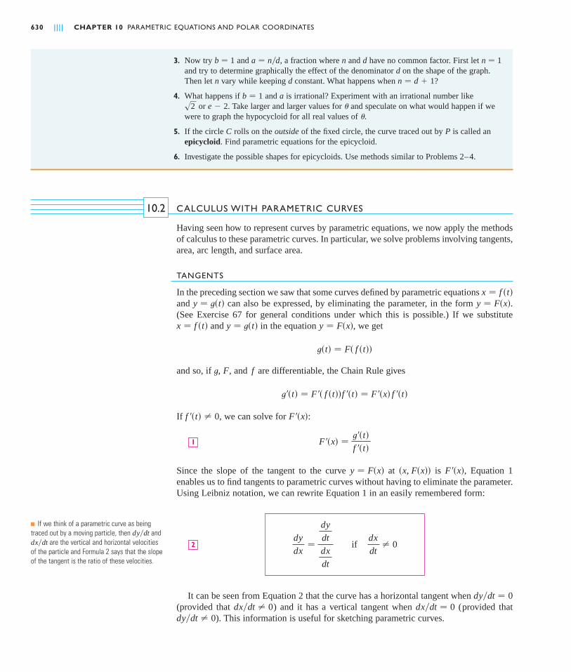
In the preceding section we saw that some curves defined by parametric equations and can also be expressed, by eliminating the parameter, in the form .(See Exercise 67 for general conditions under which this is possible.) If we substitute

and in the equation , we get

and so, if , , and are differentiable, the Chain Rule gives

If , we can solve for :

Since the slope of the tangent to the curve at is , Equation 1enables us to find tangents to parametric curves without having to eliminate the parameter.Using Leibniz notation, we can rewrite Equation 1 in an easily remembered form:

It can be seen from Equation 2 that the curve has a horizontal tangent when (provided that ) and it has a vertical tangent when (provided that

). This information is useful for sketching parametric curves.dy�dt � 0dx�dt � 0dx�dt � 0

dy�dt � 0

dx

dt� 0if

dy

dx�

dy

dt

dx

dt

2

F��x��x, F�x��y � F�x�

F��x� �t��t�f ��t�

1

F��x�f ��t� � 0

t��t� � F�� f �t��f ��t� � F��x� f ��t�

fFt

t�t� � F� f �t��

y � F�x�y � t�t�x � f �t�

y � F�x�y � t�t�x � f �t�

10.2

N If we think of a parametric curve as beingtraced out by a moving particle, then and

are the vertical and horizontal velocitiesof the particle and Formula 2 says that the slopeof the tangent is the ratio of these velocities.

dx�dtdy�dt

As we know from Chapter 4, it is also useful to consider . This can be found byreplacing y by dy�dx in Equation 2:

EXAMPLE 1 A curve is defined by the parametric equations ,(a) Show that has two tangents at the point (3, 0) and find their equations.(b) Find the points on where the tangent is horizontal or vertical.(c) Determine where the curve is concave upward or downward.(d) Sketch the curve.

SOLUTION(a) Notice that when or . Therefore thepoint on arises from two values of the parameter, and . Thisindicates that crosses itself at . Since

the slope of the tangent when is , so the equa-tions of the tangents at are

(b) has a horizontal tangent when , that is, when and .Since , this happens when , that is, . The correspondingpoints on are and (1, 2). has a vertical tangent when , that is,

. (Note that there.) The corresponding point on is (0, 0).

(c) To determine concavity we calculate the second derivative:

Thus the curve is concave upward when and concave downward when .

(d) Using the information from parts (b) and (c), we sketch in Figure 1. M

EXAMPLE 2(a) Find the tangent to the cycloid , at the pointwhere . (See Example 7 in Section 10.1.)(b) At what points is the tangent horizontal? When is it vertical?

SOLUTION(a) The slope of the tangent line is

dy

dx�

dy�d�

dx�d��

r sin �

r �1 � cos ��

sin �

1 � cos �

� � ��3y � r �1 � cos ��x � r �� sin ��

V

C

t � 0t � 0

d 2y

dx 2 �

d

dt �dy

dx�dx

dt

�

3

2 �1 �

1

t 2�2t

�3�t 2 � 1�

4t 3

Cdy�dt � 0t � 0dx�dt � 2t � 0C�1, �2�C

t � 1t 2 � 1dy�dt � 3t 2 � 3dx�dt � 0dy�dt � 0dy�dx � 0C

y � �s3 �x � 3�andy � s3 �x � 3�

�3, 0�dy�dx � 6�(2s3 ) � s3 t � s3

dy

dx�

dy�dt

dx�dt�

3t 2 � 3

2t�

3

2 �t �

1

t ��3, 0�C

t � �s3 t � s3 C�3, 0�t � s3 t � 0y � t 3 � 3t � t�t 2 � 3� � 0

CC

y � t 3 � 3t.x � t 2C

d 2y

dx 2 �d

dx �dy

dx� �

d

dt �dy

dx�dx

dt

d 2y�dx 2

| Note thatd 2y

dx2 �

d 2y

dt 2

d 2x

dt 2

SECTION 10.2 CALCULUS WITH PARAMETRIC CURVES | | | | 631

0

y

x

(3, 0)

(1, _2)

(1, 2)

t=1

t=_1

y=œ„3(x-3)

y=_ œ„3(x-3)

FIGURE 1

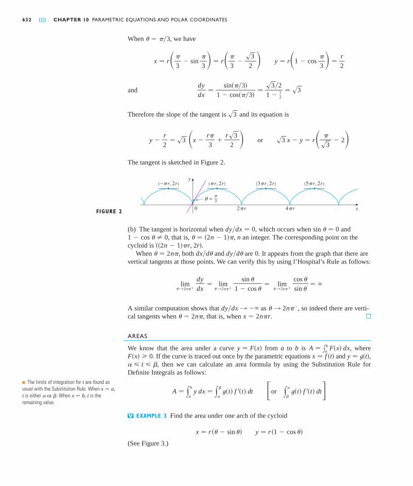
When , we have

and

Therefore the slope of the tangent is and its equation is

The tangent is sketched in Figure 2.

(b) The tangent is horizontal when , which occurs when and, that is, , an integer. The corresponding point on the

cycloid is .When , both and are 0. It appears from the graph that there are

vertical tangents at those points. We can verify this by using l’Hospital’s Rule as follows:

A similar computation shows that as , so indeed there are verti-cal tangents when , that is, when . M

AREAS

We know that the area under a curve from to is , where. If the curve is traced out once by the parametric equations and ,

, then we can calculate an area formula by using the Substitution Rule forDefinite Integrals as follows:

EXAMPLE 3 Find the area under one arch of the cycloid

(See Figure 3.)

y � r �1 � cos ��x � r �� sin ��

V

�or y

� t�t� f ��t� dt�A � y

b

a y dx � y

�

t�t� f ��t� dt

� t � �y � t�t�x � f �t�F�x� 0

A � xba F�x� dxbay � F�x�

x � 2n�r� � 2n�� l 2n��dy�dx l ��

lim� l

2n�� dy

dx� lim

� l

2n��

sin �

1 � cos �� lim

� l

2n�� cos �

sin ��

dy�d�dx�d�� 2n��2n � 1��r, 2r�

n� � �2n � 1��1 � cos � � 0sin � � 0dy�dx � 0

FIGURE 2 0

y

x2πr 4πr

(πr, 2r)(_πr, 2r) (3πr, 2r) (5πr, 2r)

π

3¨=

s3 x � y � r� �

s3 � 2�ory �r

2� s3 �x �

r�

3�

rs3

2 �s3

dy

dx�

sin��3�1 � cos��3�

�s3 �2

1 �12

� s3

y � r�1 � cos �

3 � �r

2x � r��

3� sin

�

3 � � r��

3�

s3

2 �� 3


N The limits of integration for are found asusual with the Substitution Rule. When

is either . When is the remaining value.

x � b, t or �tx � a,

t

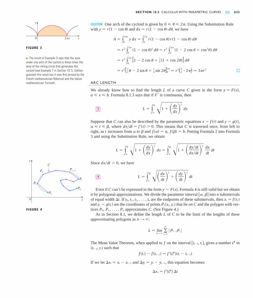
SOLUTION One arch of the cycloid is given by . Using the Substitution Rulewith and , we have

M

ARC LENGTH

We already know how to find the length of a curve given in the form ,. Formula 8.1.3 says that if is continuous, then

Suppose that can also be described by the parametric equations and ,, where . This means that is traversed once, from left to

right, as increases from to and , . Putting Formula 2 into Formula3 and using the Substitution Rule, we obtain

Since , we have

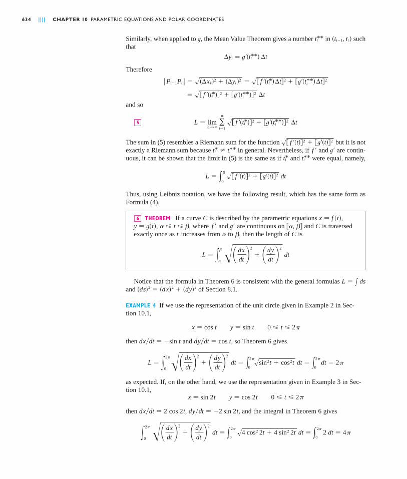
Even if can’t be expressed in the form , Formula 4 is still valid but we obtainit by polygonal approximations. We divide the parameter interval into n subintervalsof equal width . If , , , . . . , are the endpoints of these subintervals, then and are the coordinates of points that lie on and the polygon with ver-tices , , . . . , approximates . (See Figure 4.)

As in Section 8.1, we define the length of to be the limit of the lengths of theseapproximating polygons as :

The Mean Value Theorem, when applied to on the interval , gives a number insuch that

If we let and , this equation becomes

�xi � f ��ti*� �t

�yi � yi � yi�1�xi � xi � xi�1

f �ti� � f �ti�1� � f ��ti*��ti � ti�1��ti�1, ti�

ti*ti�1, tif

L � limnl �

�n

i�1 � Pi�1Pi �

n l �CL

CPnP1P0

CPi�xi, yi�yi � t�ti�xi � f �ti�tnt2t1t0�t

, �y � F�x�C

L � y�

�dx

dt �2

� �dy

dt �2

dt4

dx�dt � 0

L � yb

a 1 � �dy

dx�2

dx � y�

1 � �dy�dt

dx�dt�2

dx

dt dt

f �� bf �� a�tCdx�dt � f ��t� � 0 � t � �

y � t�t�x � f �t�C

L � yb

a 1 � �dy

dx�2

dx3

F�a � x � by � F�x�CL

� r 2( 32 � 2�) � 3�r 2� r 2[ 3

2 � � 2 sin � �14 sin 2�]0

2�

� r 2 y2�

0 [1 � 2 cos � �

12 �1 � cos 2��] d�

� r 2 y2�

0 �1 � cos ��2 d� � r 2 y

2�

0 �1 � 2 cos � � cos2�� d�

A � y2�r

0 y dx � y

2�

0 r �1 � cos �� r �1 � cos �� d�

dx � r �1 � cos �� d�y � r �1 � cos ��0 � � � 2�


N The result of Example 3 says that the areaunder one arch of the cycloid is three times thearea of the rolling circle that generates thecycloid (see Example 7 in Section 10.1). Galileoguessed this result but it was first proved by theFrench mathematician Roberval and the Italianmathematician Torricelli.

FIGURE 3

0

y

x2πr

0

y

x

P¸

P¡

P™ Pi _1

Pi

Pn

C

FIGURE 4

Similarly, when applied to , the Mean Value Theorem gives a number in suchthat

Therefore

and so

The sum in (5) resembles a Riemann sum for the function but it is notexactly a Riemann sum because in general. Nevertheless, if and are contin-uous, it can be shown that the limit in (5) is the same as if and were equal, namely,

Thus, using Leibniz notation, we have the following result, which has the same form asFormula (4).

THEOREM If a curve is described by the parametric equations ,, , where and are continuous on and is traversed

exactly once as increases from to , then the length of is

Notice that the formula in Theorem 6 is consistent with the general formulasand of Section 8.1.

EXAMPLE 4 If we use the representation of the unit circle given in Example 2 in Sec-tion 10.1,

then and , so Theorem 6 gives

as expected. If, on the other hand, we use the representation given in Example 3 in Sec-tion 10.1,

then , , and the integral in Theorem 6 gives

y2�

0 �dx

dt �2

� �dy

dt �2

dt � y2�

0 s4 cos2 2t � 4 sin2 2t dt � y

2�

0 2 dt � 4�

dy�dt � �2 sin 2tdx�dt � 2 cos 2t

0 � t � 2�y � cos 2tx � sin 2t

� y2�

0 dt � 2�L � y

2�

0 �dx

dt �2

� �dy

dt �2

dt � y2�

0ssin2t � cos2t dt

dy�dt � cos tdx�dt � �sin t

0 � t � 2�y � sin tx � cos t

�ds�2 � �dx�2 � �dy�2L � x ds

L � y�

�dx

dt �2

� �dy

dt �2

dt

C�tC, �t�f � � t � �y � t�t�

x � f �t�C6

L � y�

s f ��t�2 � t��t�2 dt

ti**ti*t�f �ti* � ti**

s f ��t�2 � t��t�2

L � limn l �

�n

i�1 s f ��ti*�2 � t��ti

**�2 �t5

� s f ��ti*�2 � t��ti**�2 �t

� s f ��ti*��t2 � t��ti**��t2 � Pi�1Pi � � s��xi�2 � ��yi �2

�yi � t��ti**� �t

�ti�1, ti�ti**t


| Notice that the integral gives twice the arc length of the circle because as increasesfrom 0 to , the point traverses the circle twice. In general, when findingthe length of a curve from a parametric representation, we have to be careful to ensurethat is traversed only once as increases from to . M

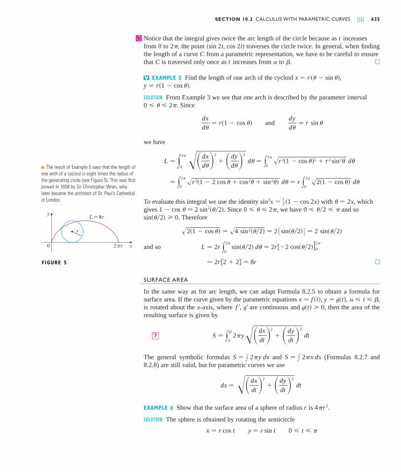
EXAMPLE 5 Find the length of one arch of the cycloid ,

SOLUTION From Example 3 we see that one arch is described by the parameter interval. Since

we have

To evaluate this integral we use the identity with , whichgives . Since , we have and so

. Therefore

and so

M

SURFACE AREA

In the same way as for arc length, we can adapt Formula 8.2.5 to obtain a formula forsurface area. If the curve given by the parametric equations , , ,is rotated about the -axis, where , are continuous and , then the area of theresulting surface is given by

The general symbolic formulas and (Formulas 8.2.7 and8.2.8) are still valid, but for parametric curves we use

EXAMPLE 6 Show that the surface area of a sphere of radius is .

SOLUTION The sphere is obtained by rotating the semicircle

0 � t � �y � r sin tx � r cos t

4�r 2r

ds � �dx

dt �2

� �dy

dt �2

dt

S � x 2�x dsS � x 2�y ds

S � y�

2�y �dx

dt �2

� �dy

dt �2

dt 7

t�t� 0t�f �x � t � �y � t�t�x � f �t�

� 2r 2 � 2 � 8r

L � 2r y2�

0 sin��2� d� � 2r �2 cos��2�]0

2�

s2�1 � cos �� s4 sin2��2� � 2 � sin��2� � � 2 sin��2�

sin��2� 00 � ��2 � �0 � � � 2�1 � cos � � 2 sin2��2�

� � 2xsin2x � 12 �1 � cos 2x�

� y2�

0 sr 2�1 � 2 cos � � cos2� � sin2�� d� � r y

2�

0 s2�1 � cos �� d�

L � y2�

0 � dx

d��2

� � dy

d��2

d� � y2�

0 sr 2�1 � cos ��2 � r 2 sin2� d�

dy

d�� r sin �and

dx

d�� r�1 � cos ��

0 � � � 2�

y � r�1 � cos ��.x � r �� sin ��V

�tCC

�sin 2t, cos 2t�2�t


N The result of Example 5 says that the length ofone arch of a cycloid is eight times the radius ofthe generating circle (see Figure 5). This was firstproved in 1658 by Sir Christopher Wren, wholater became the architect of St. Paul’s Cathedralin London.

FIGURE 5

0

y

x2πr

r

L=8r

about the -axis. Therefore, from Formula 7, we get

M� 2�r 2��cos t�]0

�

� 4�r 2� 2�r 2 y�

0 sin t dt

� 2� y�

0 r sin t � r dt� 2� y

�

0 r sin t sr 2�sin2t � cos2t� dt

S � y�

0 2�r sin t s��r sin t�2 � �r cos t�2 dt

x


19. ,

20. ,

; 21. Use a graph to estimate the coordinates of the rightmost pointon the curve , . Then use calculus to find theexact coordinates.

; 22. Use a graph to estimate the coordinates of the lowest point andthe leftmost point on the curve , . Thenfind the exact coordinates.

; 23–24 Graph the curve in a viewing rectangle that displays all theimportant aspects of the curve.

,

24. ,

Show that the curve , has two tangentsat and find their equations. Sketch the curve.

; 26. Graph the curve , todiscover where it crosses itself. Then find equations of bothtangents at that point.

27. (a) Find the slope of the tangent line to the trochoid, in terms of . (See Exer-

cise 40 in Section 10.1.)(b) Show that if , then the trochoid does not have a

vertical tangent.

28. (a) Find the slope of the tangent to the astroid ,in terms of . (Astroids are explored in the

Laboratory Project on page 629.)(b) At what points is the tangent horizontal or vertical?(c) At what points does the tangent have slope 1 or ?

29. At what points on the curve , does thetangent line have slope ?

30. Find equations of the tangents to the curve ,that pass through the point .

Use the parametric equations of an ellipse, ,, , to find the area that it encloses.0 � � � 2�y � b sin �

x � a cos �31.

�4, 3�y � 2t 3 � 1x � 3t 2 � 1

1y � 1 � 4t � t 2x � 2t 3

�1

�y � a sin3�x � a cos3�

d � r

�y � r � d cos �x � r� � d sin �

y � sin t � 2 sin 2tx � cos t � 2 cos 2t

�0, 0�y � sin t cos tx � cos t25.

y � 2t 2 � tx � t 4 � 4t 3 � 8t 2

y � t 3 � tx � t 4 � 2t 3 � 2t 223.

y � t � t 4x � t 4 � 2t

y � e tx � t � t 6

y � 2 sin �x � cos 3�

y � sin 2�x � 2 cos �1–2 Find .

1. , 2. ,

3–6 Find an equation of the tangent to the curve at the point corre-sponding to the given value of the parameter.

3. , ;

4. , ;

, ;

6. , ;

7–8 Find an equation of the tangent to the curve at the given pointby two methods: (a) without eliminating the parameter and (b) byfirst eliminating the parameter.

7. , ;

8. , ;

; 9–10 Find an equation of the tangent(s) to the curve at the givenpoint. Then graph the curve and the tangent(s).

9. , ;

10. , ;

11–16 Find and . For which values of is the curveconcave upward?

, 12. ,

13. , 14. ,

15. , ,

16. , ,

17–20 Find the points on the curve where the tangent is horizontalor vertical. If you have a graphing device, graph the curve to checkyour work.

17. ,

18. , y � 2t 3 � 3t 2 � 1x � 2t 3 � 3t 2 � 12t

y � t 3 � 12tx � 10 � t 2

0 � t � �y � cos tx � cos 2 t

0 � t � 2�y � 3 cos tx � 2 sin t

y � t � ln tx � t � ln ty � t � e� tx � t � e t

y � t 2 � 1x � t 3 � 12ty � t 2 � t 3x � 4 � t 211.

td 2 y�dx 2dy�dx

��1, 1�y � sin t � sin 2tx � cos t � cos 2t

�0, 0�y � t 2 � tx � 6 sin t

(1, s2)y � sec �x � tan �

�1, 3�y � t 2 � 2x � 1 � ln t

� � 0y � sin � � cos 2�x � cos � � sin 2�

t � 1y � t � ln t 2x � est

5.

t � 1y � 1 � t 2x � t � t�1

t � �1y � t 3 � tx � t 4 � 1

y � st e�tx � 1�ty � t 2 � tx � t sin t

dy�dx

EXERCISES10.2

49. Use Simpson’s Rule with to estimate the length of thecurve , , .

50. In Exercise 43 in Section 10.1 you were asked to derive theparametric equations , for thecurve called the witch of Maria Agnesi. Use Simpson’s Rulewith to estimate the length of the arc of this curvegiven by .

51–52 Find the distance traveled by a particle with position as varies in the given time interval. Compare with the length ofthe curve.

51. , ,

52. , ,

53. Show that the total length of the ellipse ,, , is

where is the eccentricity of the ellipse , where.

54. Find the total length of the astroid , ,where

55. (a) Graph the epitrochoid with equations

What parameter interval gives the complete curve?(b) Use your CAS to find the approximate length of this

curve.

56. A curve called Cornu’s spiral is defined by the parametricequations

where and are the Fresnel functions that were introducedin Chapter 5.(a) Graph this curve. What happens as and as

?(b) Find the length of Cornu’s spiral from the origin to the

point with parameter value .

57–58 Set up an integral that represents the area of the surfaceobtained by rotating the given curve about the -axis. Then useyour calculator to find the surface area correct to four decimalplaces.

57. , ,

58. , , 0 � t � ��3y � sin 3tx � sin2t

0 � t � 1y � �t 2 � 1�e tx � 1 � te t

x

t

t l ��t l �

SC

y � S�t� � yt

0 sin��u 2�2� du

x � C�t� � yt

0 cos��u 2�2� du

CAS

y � 11 sin t � 4 sin�11t�2�

x � 11 cos t � 4 cos�11t�2�

CAS

a � 0.y � a sin3�x � a cos3�

c � sa 2 � b 2 )(e � c�ae

L � 4a y��2

0 s1 � e 2 sin2� d�

a � b � 0y � b cos �x � a sin �

0 � t � 4�y � cos tx � cos2t

0 � t � 3�y � cos2tx � sin2t

t�x, y�

��4 � � � ��2n � 4

y � 2a sin2�x � 2a cot �

�6 � t � 6y � t � e tx � t � e tn � 632. Find the area enclosed by the curve , and

the .

33. Find the area enclosed by the and the curve , .

34. Find the area of the region enclosed by the astroid, . (Astroids are explored in the Labo-

ratory Project on page 629.)

35. Find the area under one arch of the trochoid of Exercise 40 inSection 10.1 for the case .

36. Let be the region enclosed by the loop of the curve inExample 1.(a) Find the area of .(b) If is rotated about the -axis, find the volume of the

resulting solid.(c) Find the centroid of .

37–40 Set up an integral that represents the length of the curve.Then use your calculator to find the length correct to four decimalplaces.

37. , ,

38. , ,

39. , ,

40. , ,

41–44 Find the exact length of the curve.

, ,

42. , ,

43. , ,

44. , ,

; 45–47 Graph the curve and find its length.

, ,

46. , ,

47. , ,

48. Find the length of the loop of the curve ,.y � 3t 2

x � 3t � t 3

�8 � t � 3y � 4e t�2x � e t � t

��4 � t � 3��4y � sin tx � cos t � ln(tan 12 t)0 � t � �y � e t sin tx � e t cos t45.

0 � t � �y � 3 sin t � sin 3tx � 3 cos t � cos 3t

0 � t � 2y � ln�1 � t�x �t

1 � t

0 � t � 3y � 5 � 2tx � et � e�t

0 � t � 1y � 4 � 2t 3x � 1 � 3t 241.

1 � t � 5y � st � 1x � ln t

0 � t � 2�y � t � sin tx � t � cos t

�3 � t � 3y � t 2x � 1 � e t

1 � t � 2y � 43 t 3�2x � t � t 2

�

x��

�

d � r

y

x0 a_a

_a

a

y � a sin3�x � a cos3�

y � t � t 2x � 1 � e tx-axis

y-axisy � st x � t 2 � 2t


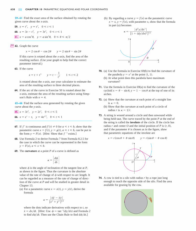
(b) By regarding a curve as the parametric curve, , with parameter , show that the formula

in part (a) becomes

70. (a) Use the formula in Exercise 69(b) to find the curvature ofthe parabola at the point .

(b) At what point does this parabola have maximumcurvature?

71. Use the formula in Exercise 69(a) to find the curvature of thecycloid , at the top of one of itsarches.

72. (a) Show that the curvature at each point of a straight line is .

(b) Show that the curvature at each point of a circle of radius is .

73. A string is wound around a circle and then unwound whilebeing held taut. The curve traced by the point at the end ofthe string is called the involute of the circle. If the circle hasradius and center and the initial position of is ,and if the parameter is chosen as in the figure, showthat parametric equations of the involute are

74. A cow is tied to a silo with radius by a rope just longenough to reach the opposite side of the silo. Find the areaavailable for grazing by the cow.

r

xO

y

r

¨ P

T

y � r �sin � � � cos ��x � r �cos � � � sin ��

��r, 0�POr

P

� � 1�rr

� � 0

y � 1 � cos �x � � � sin �

�1, 1�y � x 2

0 x

y

P

˙

� � � d 2 y�dx 2 �1 � �dy�dx�2 3�2

xy � f �x�x � xy � f �x�59–61 Find the exact area of the surface obtained by rotating the

given curve about the -axis.

59. , ,

60. , ,

, ,

; 62. Graph the curve

If this curve is rotated about the -axis, find the area of theresulting surface. (Use your graph to help find the correct parameter interval.)

63. If the curve

is rotated about the -axis, use your calculator to estimate thearea of the resulting surface to three decimal places.

64. If the arc of the curve in Exercise 50 is rotated about the -axis, estimate the area of the resulting surface using Simp-

son’s Rule with .

65–66 Find the surface area generated by rotating the givencurve about the -axis.

, ,

66. , ,

67. If is continuous and for , show that theparametric curve , , , can be put inthe form . [Hint: Show that exists.]

68. Use Formula 2 to derive Formula 7 from Formula 8.2.5 forthe case in which the curve can be represented in the form

, .

69. The curvature at a point of a curve is defined as

where is the angle of inclination of the tangent line at ,as shown in the figure. Thus the curvature is the absolutevalue of the rate of change of with respect to arc length. Itcan be regarded as a measure of the rate of change of direc-tion of the curve at and will be studied in greater detail inChapter 13.(a) For a parametric curve , , derive the

formula

where the dots indicate derivatives with respect to , so. [Hint: Use and Formula 2

to find . Then use the Chain Rule to find .]d��dsd��dt� � tan�1�dy�dx�x� � dx�dt

t

� � � x�y�� x��y� �x� 2 � y� 2 3�2

y � y�t�x � x�t�

P

�

P�

� � � d�

ds �P

a � x � by � F�x�

f �1y � F�x�a � t � by � t�t�x � f �t�a � t � bf ��t� � 0f �

0 � t � 1y � 4e t�2x � e t � t

0 � t � 5y � 2t 3x � 3t 265.

y

n � 4x

x

1 � t � 2y � t �1

t 2x � t � t 3

x

y � 2 sin � � sin 2�x � 2 cos � � cos 2�

0 � � � ��2y � a sin3�x � a cos3�61.

0 � t � 1y � 3t 2x � 3t � t 3

0 � t � 1y � t 2x � t 3

x


The Bézier curves are used in computer-aided design and are named after the French mathema-tician Pierre Bézier (1910–1999), who worked in the automotive industry. A cubic Bézier curve is determined by four control points, and , and is defined by the parametric equations

where . Notice that when we have and when we have, so the curve starts at and ends at .

1. Graph the Bézier curve with control points , , , and Then, on the same screen, graph the line segments , , and . (Exercise 31 in Section 10.1 shows how to do this.) Notice that the middle control points and don’t lieon the curve; the curve starts at , heads toward and without reaching them, and ends at

2. From the graph in Problem 1, it appears that the tangent at passes through and the tangent at passes through . Prove it.

3. Try to produce a Bézier curve with a loop by changing the second control point in Problem 1.

4. Some laser printers use Bézier curves to represent letters and other symbols. Experiment with control points until you find a Bézier curve that gives a reasonable representation of the letter C.

5. More complicated shapes can be represented by piecing together two or more Bézier curves.Suppose the first Bézier curve has control points and the second one has con-trol points . If we want these two pieces to join together smoothly, then thetangents at should match and so the points , , and all have to lie on this commontangent line. Using this principle, find control points for a pair of Bézier curves that repre-sent the letter S.

P4P3P2P3

P3, P4, P5, P6

P0, P1, P2, P3

P2P3

P1P0

P3 .P2P1P0

P2P1

P2P3P1P2P0P1

P3�40, 5�.P2�50, 42�P1�28, 48�P0�4, 1�

P3P0�x, y� � �x3, y3�t � 1�x, y� � �x0, y0 �t � 00 � t � 1

y � y0�1 � t�3 � 3y1t�1 � t�2 � 3y2t 2�1 � t� � y3t 3

x � x0�1 � t�3 � 3x1t�1 � t�2 � 3x2t 2�1 � t� � x3t 3

P3�x3, y3 �P0�x0, y0 �, P1�x1, y1�, P2�x2, y2 �,

SECTION 10.3 POLAR COORDINATES | | | | 639

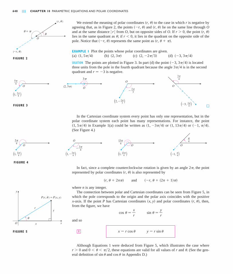
POLAR COORDINATES

A coordinate system represents a point in the plane by an ordered pair of numbers calledcoordinates. Usually we use Cartesian coordinates, which are directed distances from twoperpendicular axes. Here we describe a coordinate system introduced by Newton, calledthe polar coordinate system, which is more convenient for many purposes.

We choose a point in the plane that is called the pole (or origin) and is labeled . Thenwe draw a ray (half-line) starting at called the polar axis. This axis is usually drawn hor-izontally to the right and corresponds to the positive -axis in Cartesian coordinates.

If is any other point in the plane, let be the distance from to and let be theangle (usually measured in radians) between the polar axis and the line as in Figure 1.Then the point is represented by the ordered pair and , are called polar coordi-nates of . We use the convention that an angle is positive if measured in the counter-clockwise direction from the polar axis and negative in the clockwise direction. If ,then and we agree that represents the pole for any value of .��0, ��r � 0

P � OP

�r�r, ��POP

�POrPx

OO

10.3

xO

¨

r

polar axis

P(r, )

FIGURE 1

; BEZIER CURVESL A B O R AT O R YP R O J E C T

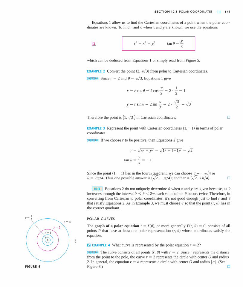
We extend the meaning of polar coordinates to the case in which is negative byagreeing that, as in Figure 2, the points and lie on the same line through and at the same distance from , but on opposite sides of . If , the point lies in the same quadrant as ; if , it lies in the quadrant on the opposite side of thepole. Notice that represents the same point as .

EXAMPLE 1 Plot the points whose polar coordinates are given.(a) (b) (c) (d)

SOLUTION The points are plotted in Figure 3. In part (d) the point is locatedthree units from the pole in the fourth quadrant because the angle is in the secondquadrant and is negative.

M

In the Cartesian coordinate system every point has only one representation, but in thepolar coordinate system each point has many representations. For instance, the point

in Example 1(a) could be written as or or .(See Figure 4.)

In fact, since a complete counterclockwise rotation is given by an angle 2 , the pointrepresented by polar coordinates is also represented by

where is any integer.The connection between polar and Cartesian coordinates can be seen from Figure 5, in

which the pole corresponds to the origin and the polar axis coincides with the positive -axis. If the point has Cartesian coordinates and polar coordinates , then,

from the figure, we have

and so

Although Equations 1 were deduced from Figure 5, which illustrates the case whereand , these equations are valid for all values of and (See the gen-

eral definition of and in Appendix D.)cos �sin ��.r0 � � � ��2r � 0

y � r sin �x � r cos �1

sin � �y

rcos � �

x

r

�r, ��x, y�Px

n

��r, � � �2n � 1��and�r, � � 2n��

�r, ��

O

13π4

”1, ’13π

4

O

_3π4

”1, _ ’3π4

O

”1, ’5π4

5π4

FIGURE 4

O

”_1, ’π4

π4

��1, ��4��1, 13��4��1, �3��4��1, 5��4�

O

”_3, ’3π4

3π

4

(2, 3π)O

3π

”1, ’5π4

5π

4O

FIGURE 3

O

”2, _ ’2π3

2π

3_

r � �33��4

��3, 3��4�

��3, 3��4��2, �2��3��2, 3��1, 5��4�

�r, � � ��r, ��r � 0�

�r, ��r � 0OO� r �O�r, ��r, ��

r�r, ��


(_r, ¨)

O

¨

(r, ¨ )

¨+π

FIGURE 2

O

y

x

¨

x

yr

P (r, )=P(x, y)

FIGURE 5

Equations 1 allow us to find the Cartesian coordinates of a point when the polar coor-dinates are known. To find and when and are known, we use the equations

which can be deduced from Equations 1 or simply read from Figure 5.

EXAMPLE 2 Convert the point from polar to Cartesian coordinates.

SOLUTION Since and , Equations 1 give

Therefore the point is in Cartesian coordinates. M

EXAMPLE 3 Represent the point with Cartesian coordinates in terms of polarcoordinates.

SOLUTION If we choose to be positive, then Equations 2 give

Since the point lies in the fourth quadrant, we can choose or. Thus one possible answer is ; another is . M

Equations 2 do not uniquely determine when and are given because, as increases through the interval , each value of occurs twice. Therefore, inconverting from Cartesian to polar coordinates, it’s not good enough just to find and that satisfy Equations 2. As in Example 3, we must choose so that the point lies inthe correct quadrant.

POLAR CURVES

The graph of a polar equation , or more generally , consists of allpoints that have at least one polar representation whose coordinates satisfy theequation.

EXAMPLE 4 What curve is represented by the polar equation ?

SOLUTION The curve consists of all points with . Since represents the distancefrom the point to the pole, the curve represents the circle with center and radius. In general, the equation represents a circle with center and radius . (See

Figure 6.) M

� a �Or � a2Or � 2

rr � 2�r, ��

r � 2V

�r, ��PF�r, �� 0r � f ��

�r, ��r

tan �0 � � � 2��yx�NOTE

�s2 , 7��4�(s2 , ��4)� � 7��4� � ��4�1, �1�

tan � �y

x� �1

r � sx 2 � y 2 � s12 � ��1�2 � s2

r

�1, �1�

(1, s3 )

y � r sin � � 2 sin �

3� 2 �

s3

2� s3

x � r cos � � 2 cos �

3� 2 �

1

2� 1

� � ��3r � 2

�2, ��3�

tan � �y

xr 2 � x 2 � y 22

yx�r


FIGURE 6

x

r=1

2

r=1

r=2

r=4

EXAMPLE 5 Sketch the polar curve .

SOLUTION This curve consists of all points such that the polar angle is 1 radian. It is the straight line that passes through and makes an angle of 1 radian with the polaraxis (see Figure 7). Notice that the points on the line with are in the firstquadrant, whereas those with are in the third quadrant. M

EXAMPLE 6(a) Sketch the curve with polar equation .(b) Find a Cartesian equation for this curve.

SOLUTION(a) In Figure 8 we find the values of for some convenient values of and plot thecorresponding points . Then we join these points to sketch the curve, which appearsto be a circle. We have used only values of between 0 and , since if we let increasebeyond , we obtain the same points again.

(b) To convert the given equation to a Cartesian equation we use Equations 1 and 2.From we have , so the equation becomes ,which gives

or

Completing the square, we obtain

which is an equation of a circle with center and radius 1. M

FIGURE 9

O

y

x2

¨

r

P

Q

�1, 0�

�x � 1�2 � y 2 � 1

x 2 � y 2 � 2x � 02x � r 2 � x 2 � y 2

r � 2x�rr � 2 cos �cos � � x�rx � r cos �

FIGURE 8Table of values andgraph of r=2 cos

(2, 0)

2

”_1, ’2π3

”0, ’π2

”1, ’π3

”œ„, ’π4

”œ„, ’π6

3

”_ œ„, ’5π6

3

”_ œ„, ’3π4

2

��

�r, ��r

r � 2 cos �

r � 0r � 0�r, 1�

O��r, ��

� � 1


Ox

1

(_1, 1)

(_2, 1)

(1, 1)

(2, 1)

(3, 1)

¨=1

FIGURE 7

0 2

10

�1

�2��s35��6�s23��4

2��3��2��3

s2��4s3��6

r � 2 cos ��

N Figure 9 shows a geometrical illustration that the circle in Example 6 has the equation

. The angle is a right angle(Why?) and so .r�2 � cos �

OPQr � 2 cos �

EXAMPLE 7 Sketch the curve .

SOLUTION Instead of plotting points as in Example 6, we first sketch the graph ofin Cartesian coordinates in Figure 10 by shifting the sine curve up one

unit. This enables us to read at a glance the values of that correspond to increasing values of . For instance, we see that as increases from 0 to , (the distance from )increases from 1 to 2, so we sketch the corresponding part of the polar curve in Figure11(a). As increases from to , Figure 10 shows that decreases from 2 to 1, so wesketch the next part of the curve as in Figure 11(b). As increases from to ,

decreases from 1 to 0 as shown in part (c). Finally, as increases from to , increases from 0 to 1 as shown in part (d). If we let increase beyond or decrease

beyond 0, we would simply retrace our path. Putting together the parts of the curve fromFigure 11(a)–(d), we sketch the complete curve in part (e). It is called a cardioid,because it’s shaped like a heart.

M

EXAMPLE 8 Sketch the curve .

SOLUTION As in Example 7, we first sketch , , in Cartesian coordi-nates in Figure 12. As increases from 0 to , Figure 12 shows that decreases from1 to 0 and so we draw the corresponding portion of the polar curve in Figure 13 (indi-cated by !). As increases from to , goes from 0 to . This means that thedistance from increases from 0 to 1, but instead of being in the first quadrant this por-tion of the polar curve (indicated by @) lies on the opposite side of the pole in the thirdquadrant. The remainder of the curve is drawn in a similar fashion, with the arrows andnumbers indicating the order in which the portions are traced out. The resulting curvehas four loops and is called a four-leaved rose.

M

¨=0¨=π

⑧

¨=3π4

¨=π2

¨=π4

FIGURE 12r=cos 2¨ in Cartesian coordinates

FIGURE 13Four-leaved rose r=cos 2¨

r

1

¨2ππ 5π4

π2

π4

3π4

3π2

7π4

!

@ # ^ &

% *$!

@ #

$

%

& ^

O�1r��2��4�

r��4�0 � � � 2�r � cos 2�

r � cos 2�

(a) (b) (c) (d) (e)

FIGURE 11 Stages in sketching the cardioid r=1+sin ¨

O¨=π

¨=π2

O

¨=π

¨=3π2

O

¨=2π

¨=3π2

O

O ¨=0

¨=π2

1

2

2��r2�3��2�r

3��2��r��2�

Or��2��r

r � 1 � sin �

r � 1 � sin �V


FIGURE 10r=1+sin in Cartesian coordinates,0¯¨¯2π

0

r

1

2

¨π 2π3π2

π2

Module 10.3 helps you see howpolar curves are traced out by showing animations similar to Figures 10–13.

TEC

Documents

PARAMETRIC EQUATIONS AND POLAR COORDINATES · 2017-11-17 · CURVES DEFINED BY PARAMETRIC EQUATIONS Imagine that a particle moves along the curve shown in Figure 1. It is impossible