Parametric Estimating –Multiple Regression

The term “multiple” regression is used here to describe an equation with two or more independent (X) variables. This job aid specifically addresses the statistics and issues associated with equations involving multiple X variables, beginning with a fairly concise overview of the topics, and then offering somewhat more expanded explanations.

This job aid is intended as a complement to the Linear Regression job aid which outlines the process of developing a cost estimating relationship (CER), addresses some of the common goodness of fit statistics, and provides an introduction to some of the issues concerning outliers. You will see the steps in that job aid cited as Steps 1–13, with the Multiple Regression job aid picking up at Step 14.

Multiple Regression

Multiple Regression (continued)

These topics are addressed in the Linear Regression job aid, and they are provided here as a reminder.

The first six are the fundamental steps in developing an estimating relationship regardless of the number of X variables in the equation, and whether dealing with linear or nonlinear relationships.

Items 7, 8, and 9 address the T-statistic, standard error, coefficient of variation, and the R squared.

Outliers and influential observations are discussed in 10, 11, and 12.

Number 13 introduces the idea of residual analysis, the expectation for the behavior of the residuals, and what patterns in the residuals might suggest.

Developing Cost Estimating Relationships

Expectation. In one case it was determined that factory maintenance hours were a function of both direct manufacturing labor hours and the amount of factory floor space, so the equation would need to include both variables.

Analyst preference. Let’s say you were buying a car, and the engine horsepower, trunk capacity, and the self-navigation capability were important in your decision model. Essentially you want a model with a performance variable, size variable, and a technology variable because capturing all of those characteristics is important to you.

Statistics. One motivation for adding variables to a model is to generate an equation that better fits the data, consequently predicting better, as indicated by a lower standard error.

Outliers. In some circumstances an apparent outlier could be an indication of a missing cost driver in the equation.

Why include additional X variables?

Regression works in a similar manner such that each additional X variable further tailors the equation to the sample data set, and, in doing so, reduces the applicability of the sample equation to the general population. If the sample is sufficiently large, adding X variables is of little consequence, however, for smaller sample sizes there is need for concern.

The number of X variables in the equation with respect to sample size is reflected in the calculation of the “degrees of freedom” (DF) associated with the Sum of Squared Errors (SSE). The DF are the difference between the sample size (n) and the number of coefficients (p) such that DF = n – p.

If you were buying clothes, you could buy clothes of a general size, or clothes that have been tailored to some extent, or clothes custom-tailored to fit you. With each tailoring the clothes are less likely to fit people in general, but rather a smaller subset.

The coefficients (p) refer to the intercept, and the slope associated with each X variable. As an X variable is added to the equation, another degree of freedom is lost. Experts assert that there is some minimum DF necessary if the sample equation is to be a useful proxy for the population equation. That minimum DF is left to estimator judgment.

Constraints on the Number of X variables

If we selected our independent (X) variables with the expectation that there was a causal relationship between them and the dependent (Y) variable, then we would hope to find correlation between the Y and X variables as well. However, it would be ideal if our independent variables were independent of each other, meaning no correlation between them.

One measure of correlation between two variables is the Coefficient of Correlation (R). Applications such as Excel can generate a pairwise correlation matrix that reports the R value between any pair of variables in the data set.

The R value can range from (-1), indicating two variables are perfectly inversely correlated, to (+1), indicating two variables are perfectly positively correlated. An R value of zero indicates that two variables are statistically independent of each other.

Strong correlation between the X variables should be noted and investigated. It’s also important to note whether a similar relationship exists between those same X variables for what you are estimating (e.g. Thrust and Weight are highly correlated in our example, so there should be a similar Thrust to Weight relationship in what we are estimating).

Correlation between the X variables

Picture that the circles represent the variation in each variable. The area where the X and Y variables overlap is the variation in Y that can be explained by the variation in that X. When the two X variables overlap Y, but not each other, each X variable is explaining a different portion of the variation in Y.

Where the X variables overlap Y and each other, the X variables are explaining the same variation in Y. Not only is this unproductive, but the fact that one X variable essentially eclipses the other X variable causes the estimates of the coefficients (slopes) of both the X variables to be less accurate than if the two X variables had not been correlated.

Other possible effects of the correlation between the X variables can be a change in the sign on the slope of one of the X variables, or for the T-statistic on one or both variables to be insignificant despite a strong correlation between the X and Y variables.

The point at which the correlation becomes harmful is a matter of judgment, but a reasonable rule of thumb would be when the absolute value of R between the two X variables is greater than (0.70). The problem becomes more complex as more X variables are introduced into the equation.

Multicollinearity and the Equation

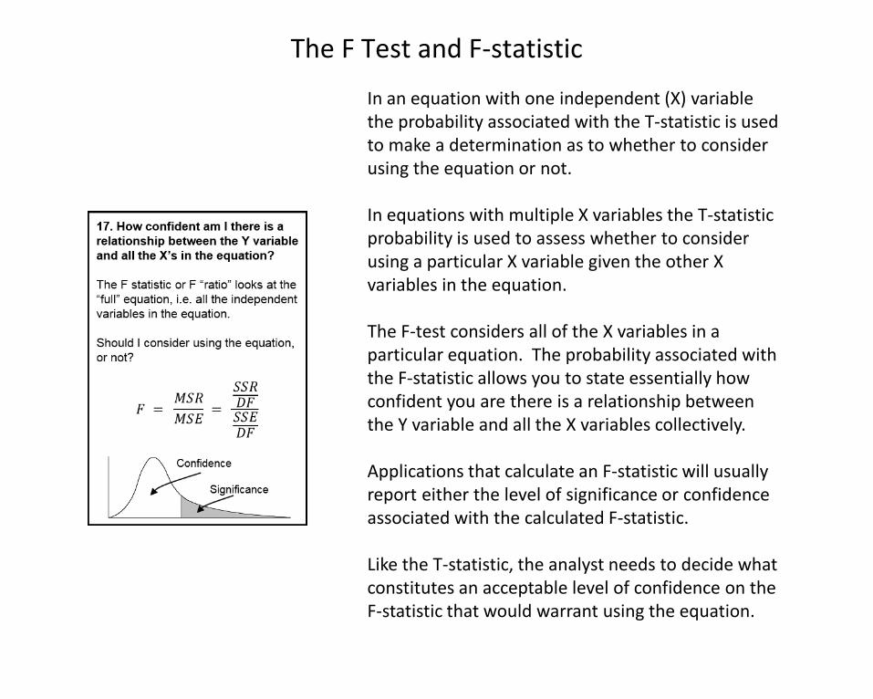
In an equation with one independent (X) variable the probability associated with the T-statistic is used to make a determination as to whether to consider using the equation or not.

In equations with multiple X variables the T-statistic probability is used to assess whether to consider using a particular X variable given the other X variables in the equation.

The F-test considers all of the X variables in a particular equation. The probability associated with the F-statistic allows you to state essentially how confident you are there is a relationship between the Y variable and all the X variables collectively.

Applications that calculate an F-statistic will usually report either the level of significance or confidence associated with the calculated F-statistic.

Like the T-statistic, the analyst needs to decide what constitutes an acceptable level of confidence on the F-statistic that would warrant using the equation.

The F Test and F-statistic

When there are two or more comparable equations available to estimate the same element of cost, some analysts might prefer to use the simplest of the equations, while other analysts might favor the equation that captures the most characteristics.

Another consideration, this in regard to correlation, is whether to consider using highly correlated X variables together in the same equation.

As was previously mentioned, in an equation with multiple X variables, the F-statistic assesses the overall relationship between the Y variable and collectively all of the X variables in the equation.

The T-stat measures the marginal contribution of a particular X variable in the equation, given the other X variables are already present in the equation. The diagram on the upper left depicts the contribution X2 makes to the equation (the shaded area) taking into account X1 is already in the equation. Likewise, in the lower right is a depiction of the contribution that X1 makes to the equation taking into account that that X2 is already in the equation. The T-stat probability can be used to determine whether to include an X variable in a particular combination.

The T-statistic in a Multiple X Equation

The marginal contribution or marginal utility of an X variable as measured by the T-statistic can perhaps best be evidenced by considering an alternative means of calculating the T-stat, and that as the square root of the Partial F statistic for that variable.

The Partial F for X2 is calculated by taking the difference between the amount of the variation in Y explained by X1 and X2 combined (SSR Full) and the amount of the variation in Y explained by X1 alone (SSR Reduced). The difference (shaded) between the SSRs is the marginal contribution that X2 makes to the equation.

Calculating the T-statistic in a Multiple X Equation

By comparison, the Standard Error (SE) can actually worsen (increase) when a variable is added to the equation. The SE is calculated by taking the square root of the SSE/(n – p). When an X is added to the equation, “p” the number of parameters in the equation, increases by one, thereby reducing (n – p) by one. The effect is that if an X is added to the equation that does not significantly reduce the SSE, then SE actually increases (worsens).

The R squared though, does not consider or “adjust for” (n – p). Subsequently it is not a reliable indicator of the benefit of adding an X variable to the equation.

R squared represents the variation in the dependent variable being explained by the independent variable or variables. As noted in the Linear job aid it can be calculated as (SSR/SST) or as (1 – SSE/SST). (Recall that SSR is the explained variation and SSE is the unexplained variation.) A shortcoming to the R squared calculation is that with the addition of an X variable to the equation the R squared will either increase or remain the same, it cannot worsen.

The “R squared adjusted” or “adjusted R squared” adjusts for the change in (n – p). In contrast to the R squared, the adjusted R squared will actually decrease if an X variable is added to the equation that does not significantly reduce the SSE.

The Adjusted R squared

We have a data set of aircraft wheel assemblies. We scatterplot the data and notice what appears to be two groupings in the data which we decide to categorize as being either small or large wheel assemblies. Both groups appear to follow a similar linear relationship (i.e. a line fit through one group would be parallel to a line fit through the other group), but the two groups appear to have different intercepts.

It can be said that not everything that counts can be counted. Some cost drivers can be easily quantified and measured, while others are more qualitative or categorical in nature such as manned and unmanned vehicles, guided and unguided bombs, gasoline and diesel engines, wheeled and tracked vehicles, or sizes such as small, medium, and large. One means of capturing these types of characteristics is to construct what are often called dummy, categorical, or qualitative X variables.

Quantifying a Qualitative Variable

We decide to construct an X variable named Large, and we assign the smaller wheels a value of zero, and the larger wheels a value of one. We run a linear regression using both Diameter and Large as our independent variables:

Price = - 9,552 + 1,741 (Diameter) + 13,517 (Large)

When estimating a small diameter wheel assembly the value for Large would be zero, giving us:

Price = - 9,552 + 1,741 (Diameter)

When estimating a large diameter wheel assembly the value for Large would be one (1), giving us:

Price = - 9,552 + 1,741 (Diameter) + 13,517 (1)

Price = 3,965 + 1,741 (Diameter)

Both the Large and Small diameter wheels have the same slope, but different intercepts. We could state that Large diameter wheels cost $13,517 more than comparable small diameter wheels.

Price Diameter Large$9,000 10 0

$14,000 14 0$18,000 16 0$42,000 22 1$45,000 24 1$49,000 26 1$54,000 28 1

Constructing Dummy Variables

As a reminder, it’s always important to note where you are estimating with respect to the data. In other words, are you estimating near the center of the data set or at the ends of the data set? How well did the equation fit the data points in the range of the data for which you are estimating? Are you estimating outside the range of the data set, and if so, how far outside the range? Do you expect the relationship between the X and Y to continue outside the range of the existing data? Do you have expert opinion to support that?

An additional “range” consideration to keep in mind is with respect to any discovery of highly correlated X variables in the data set. Whether you combine those variables in the equation or not, that relationship is a characteristic of the items in the data set. Whatever you are estimating should exhibit the same relationship between those X variables.

Estimating within the Relevant Range of the Data