Parametric Estimating –Nonlinear Regression

The term “nonlinear” regression, in the context of this job aid, is used to describe the application of linear regression in fitting nonlinear patterns in the data. The techniques outlined here are offered as samples of the types of approaches used to fit patterns that some might refer to as being “curvilinear” in nature.

This job aid is intended as a complement to the Linear Regression job aid which outlines the process of developing a cost estimating relationship (CER), addresses some of the common goodness of fit statistics, and provides an introduction to some of the issues concerning outliers. The first 6 steps from that job aid are cited on the next page for reference.

Nonlinear Regression

Nonlinear Regression (continued)

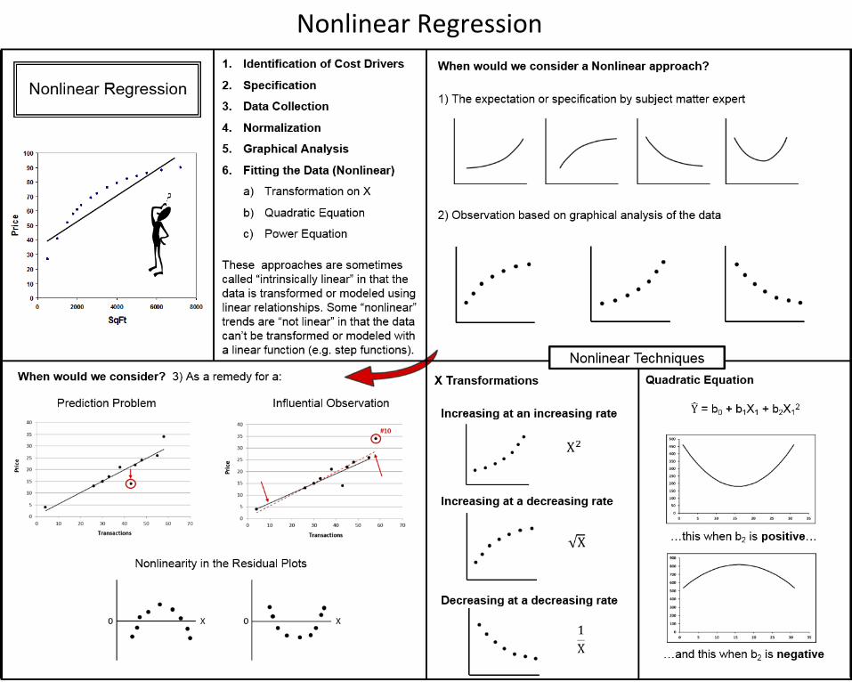
This job aid will address several techniques intended to fit patterns, such as the ones immediately below, that will be described here as being nonlinear or curvilinear (i.e. consisting of a curved line). These types of shapes are sometimes referred to as being “intrinsically linear” in that they can be “linearized” and then fit with linear equations.

For our purposes we will describe the shape below as being “not linear”. The techniques described here cannot be used to fit these types of relationships.

What do we mean by the term “nonlinear”?

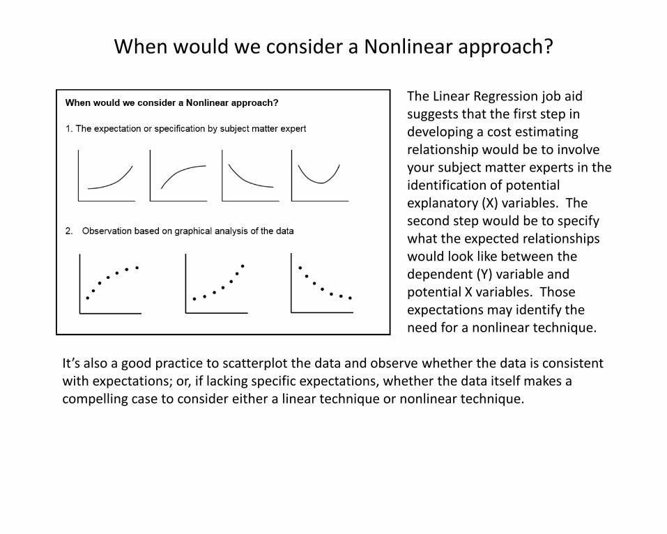
The Linear Regression job aid suggests that the first step in developing a cost estimating relationship would be to involve your subject matter experts in the identification of potential explanatory (X) variables. The second step would be to specify what the expected relationships would look like between the dependent (Y) variable and potential X variables. Those expectations may identify the need for a nonlinear technique.

When would we consider a Nonlinear approach?

It’s also a good practice to scatterplot the data and observe whether the data is consistent with expectations; or, if lacking specific expectations, whether the data itself makes a compelling case to consider either a linear technique or nonlinear technique.

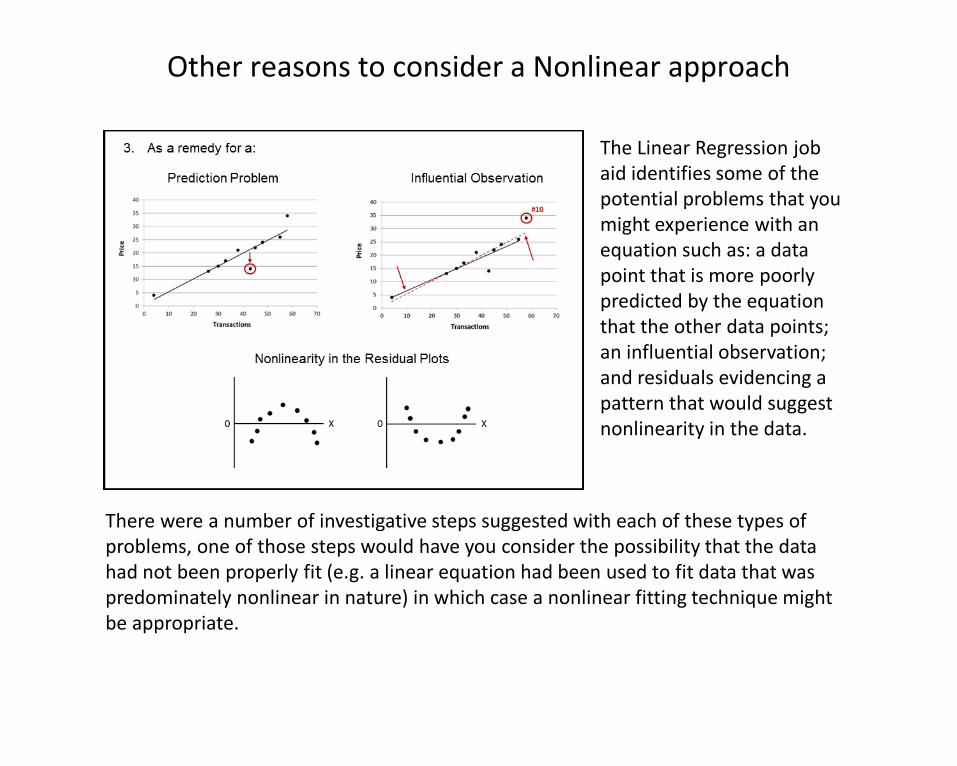
The Linear Regression job aid identifies some of the potential problems that you might experience with an equation such as: a data point that is more poorly predicted by the equation that the other data points; an influential observation; and residuals evidencing a pattern that would suggest nonlinearity in the data.

Other reasons to consider a Nonlinear approach

There were a number of investigative steps suggested with each of these types of problems, one of those steps would have you consider the possibility that the data had not been properly fit (e.g. a linear equation had been used to fit data that was predominately nonlinear in nature) in which case a nonlinear fitting technique might be appropriate.

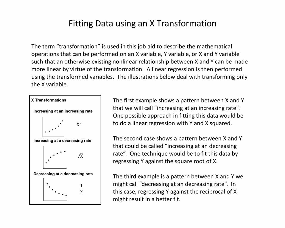
The first example shows a pattern between X and Y that we will call “increasing at an increasing rate”. One possible approach in fitting this data would be to do a linear regression with Y and X squared.

The second case shows a pattern between X and Y that could be called “increasing at an decreasing rate”. One technique would be to fit this data by regressing Y against the square root of X.

The third example is a pattern between X and Y we might call “decreasing at an decreasing rate”. In this case, regressing Y against the reciprocal of Xmight result in a better fit.

Fitting Data using an X Transformation

The term “transformation” is used in this job aid to describe the mathematical operations that can be performed on an X variable, Y variable, or X and Y variable such that an otherwise existing nonlinear relationship between X and Y can be made more linear by virtue of the transformation. A linear regression is then performed using the transformed variables. The illustrations below deal with transforming only the X variable.

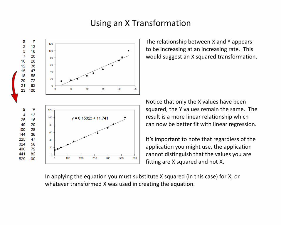
The relationship between X and Y appears to be increasing at an increasing rate. This would suggest an X squared transformation.

Notice that only the X values have been squared, the Y values remain the same. The result is a more linear relationship which can now be better fit with linear regression.

It’s important to note that regardless of the application you might use, the application cannot distinguish that the values you are fitting are X squared and not X.

Using an X Transformation

In applying the equation you must substitute X squared (in this case) for X, or whatever transformed X was used in creating the equation.

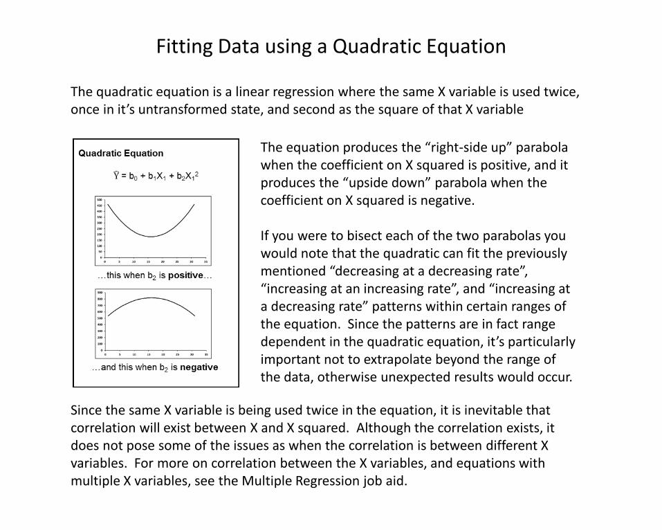
The equation produces the “right-side up” parabola when the coefficient on X squared is positive, and it produces the “upside down” parabola when the coefficient on X squared is negative.

If you were to bisect each of the two parabolas you would note that the quadratic can fit the previously mentioned “decreasing at a decreasing rate”, “increasing at an increasing rate”, and “increasing at a decreasing rate” patterns within certain ranges of the equation. Since the patterns are in fact range dependent in the quadratic equation, it’s particularly important not to extrapolate beyond the range of the data, otherwise unexpected results would occur.

Fitting Data using a Quadratic Equation

The quadratic equation is a linear regression where the same X variable is used twice, once in it’s untransformed state, and second as the square of that X variable

Since the same X variable is being used twice in the equation, it is inevitable that correlation will exist between X and X squared. Although the correlation exists, it does not pose some of the issues as when the correlation is between different X variables. For more on correlation between the X variables, and equations with multiple X variables, see the Multiple Regression job aid.

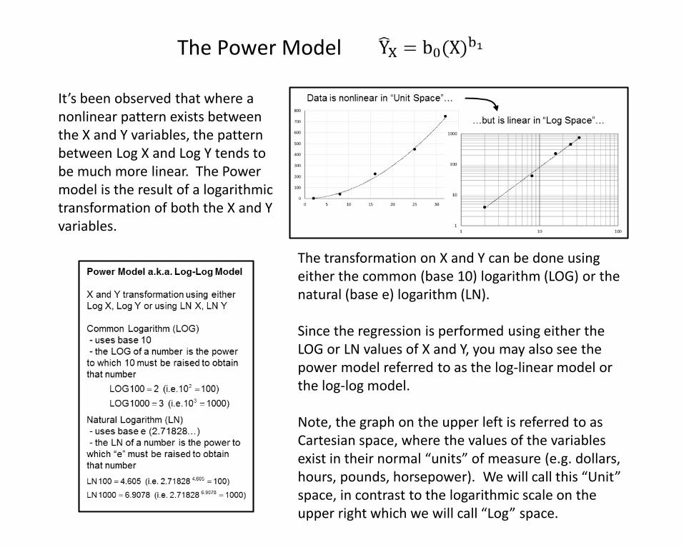
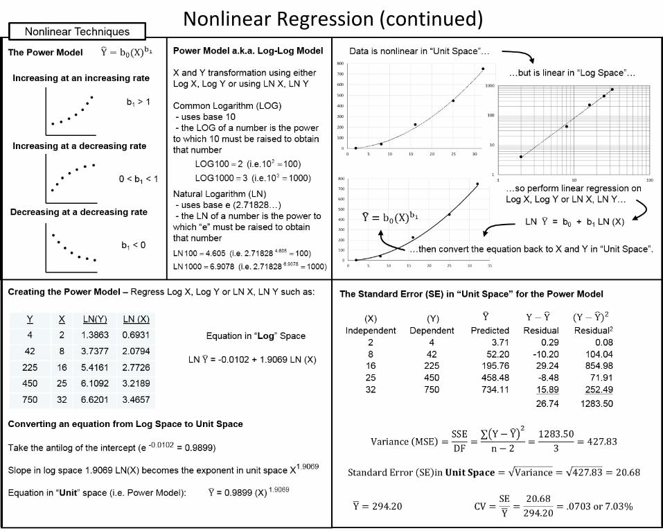
The transformation on X and Y can be done using either the common (base 10) logarithm (LOG) or the natural (base e) logarithm (LN).

Since the regression is performed using either the LOG or LN values of X and Y, you may also see the power model referred to as the log-linear model or the log-log model.

Note, the graph on the upper left is referred to as Cartesian space, where the values of the variables exist in their normal “units” of measure (e.g. dollars, hours, pounds, horsepower). We will call this “Unit” space, in contrast to the logarithmic scale on the upper right which we will call “Log” space.

The Power Model

It’s been observed that where a nonlinear pattern exists between the X and Y variables, the pattern between Log X and Log Y tends to be much more linear. The Power model is the result of a logarithmic transformation of both the X and Y variables.

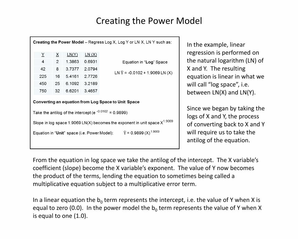
In the example, linear regression is performed on the natural logarithm (LN) of X and Y. The resulting equation is linear in what we will call “log space”, i.e. between LN(X) and LN(Y).

Since we began by taking the logs of X and Y, the process of converting back to X and Y will require us to take the antilog of the equation.

Creating the Power Model

From the equation in log space we take the antilog of the intercept. The X variable’s coefficient (slope) become the X variable’s exponent. The value of Y now becomes the product of the terms, lending the equation to sometimes being called a multiplicative equation subject to a multiplicative error term.

In a linear equation the b0 term represents the intercept, i.e. the value of Y when X is equal to zero (0.0). In the power model the b0 term represents the value of Y when X is equal to one (1.0).

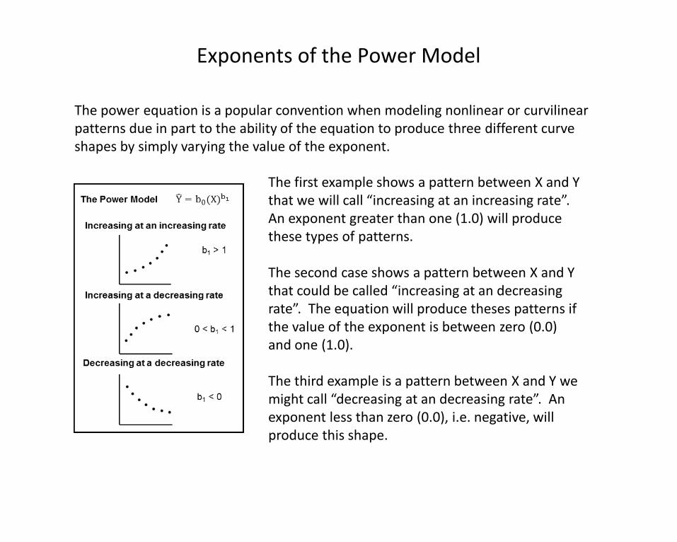
The first example shows a pattern between X and Y that we will call “increasing at an increasing rate”. An exponent greater than one (1.0) will produce these types of patterns.

The second case shows a pattern between X and Y that could be called “increasing at an decreasing rate”. The equation will produce theses patterns if the value of the exponent is between zero (0.0) and one (1.0).

The third example is a pattern between X and Y we might call “decreasing at an decreasing rate”. An exponent less than zero (0.0), i.e. negative, will produce this shape.

Exponents of the Power Model

The power equation is a popular convention when modeling nonlinear or curvilinear patterns due in part to the ability of the equation to produce three different curve shapes by simply varying the value of the exponent.

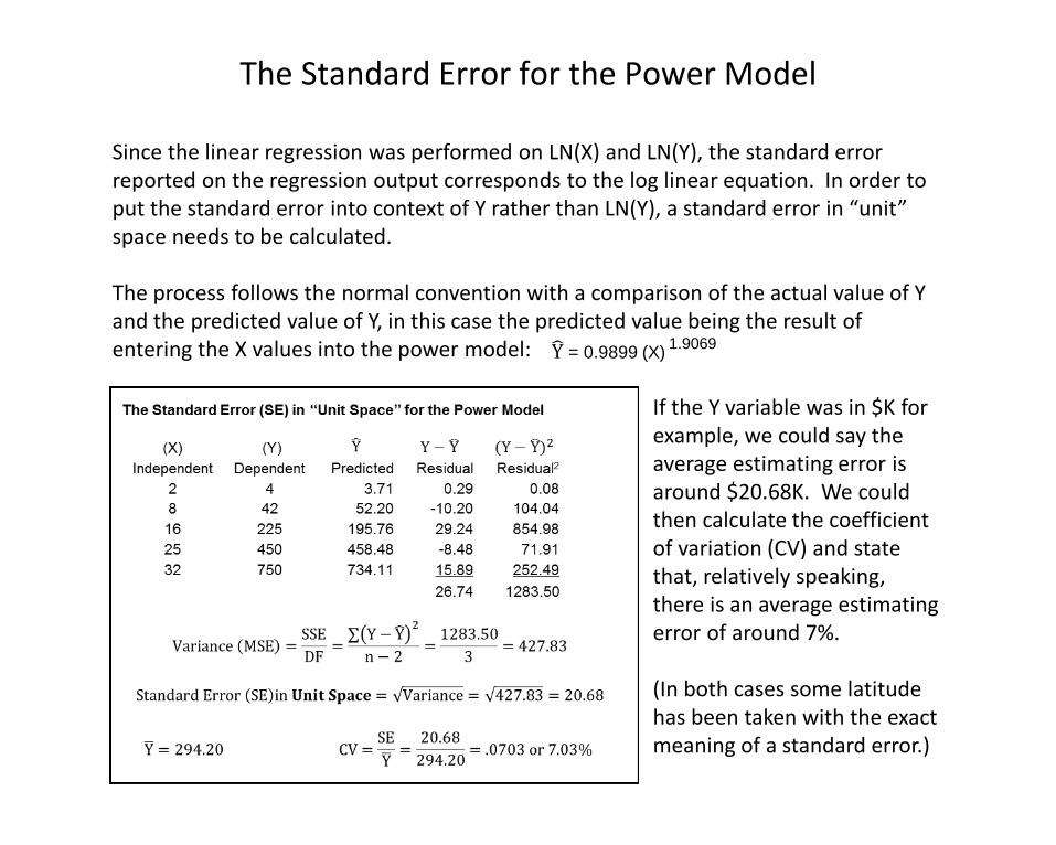
If the Y variable was in $K for example, we could say the average estimating error is around $20.68K. We could then calculate the coefficient of variation (CV) and state that, relatively speaking, there is an average estimating error of around 7%.

(In both cases some latitude has been taken with the exact meaning of a standard error.)

The Standard Error for the Power Model

Since the linear regression was performed on LN(X) and LN(Y), the standard error reported on the regression output corresponds to the log linear equation. In order to put the standard error into context of Y rather than LN(Y), a standard error in “unit” space needs to be calculated.

The process follows the normal convention with a comparison of the actual value of Y and the predicted value of Y, in this case the predicted value being the result of entering the X values into the power model: �Y = 0.9899 (X) 1.9069

The “Approximate” Standard Error for the Power Model

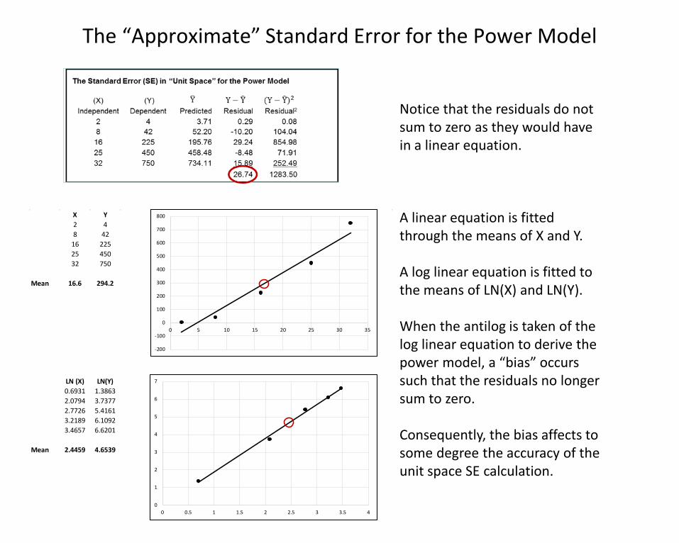
Notice that the residuals do not sum to zero as they would have in a linear equation.

A linear equation is fitted through the means of X and Y.

A log linear equation is fitted to the means of LN(X) and LN(Y).

When the antilog is taken of the log linear equation to derive the power model, a “bias” occurs such that the residuals no longer sum to zero.

Consequently, the bias affects to some degree the accuracy of the unit space SE calculation.

X Y2 48 42

16 22525 45032 750

Mean 16.6 294.2

LN (X) LN(Y)0.6931 1.38632.0794 3.73772.7726 5.41613.2189 6.10923.4657 6.6201

Mean 2.4459 4.6539

-200

-100

0

100

200

300

400

500

600

700

800

0 5 10 15 20 25 30 35

0

1

2

3

4

5

6

7

0 0.5 1 1.5 2 2.5 3 3.5 4

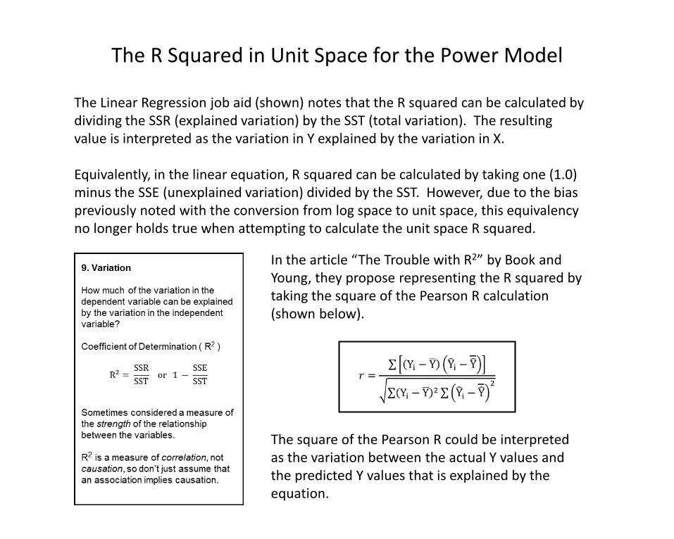
In the article “The Trouble with R2” by Book and Young, they propose representing the R squared by taking the square of the Pearson R calculation (shown below).

The square of the Pearson R could be interpreted as the variation between the actual Y values and the predicted Y values that is explained by the equation.

The R Squared in Unit Space for the Power Model

The Linear Regression job aid (shown) notes that the R squared can be calculated by dividing the SSR (explained variation) by the SST (total variation). The resulting value is interpreted as the variation in Y explained by the variation in X.

Equivalently, in the linear equation, R squared can be calculated by taking one (1.0) minus the SSE (unexplained variation) divided by the SST. However, due to the bias previously noted with the conversion from log space to unit space, this equivalency no longer holds true when attempting to calculate the unit space R squared.