Embed Size (px)
Citation preview

SSC San DiegoSan Diego, CA 92152--5001
TECHNICAL REPORT 1844November 2000
Parametric Study ofPropagation in Evaporation
Ducting and SubrefractiveConditions
Approved for public release;distribution is unlimited.
R. A. Paulus

Standard Form 298 (Rev. 8-98) Page 1 of 2
file://E:\ffcs\final\tr1844_200122031353.298.html 04/04/2001
REPORT DOCUMENTATION PAGE
1. REPORT DATE (DD-
MM-YYYY)
01-11-2000
2. REPORT TYPE
Technical Report 3. DATES COVERED (FROM - TO)
xx-xx-2000 to xx-xx-2000
4. TITLE AND SUBTITLE
Parametric Study of Propagation in Evaporation Ducting and Subrefractive Conditions
Unclassified
5a. CONTRACT NUMBER
5b. GRANT NUMBER
5c. PROGRAM ELEMENT NUMBER
6. AUTHOR(S)
Paulus, R. A. ; 5d. PROJECT NUMBER
5e. TASK NUMBER
5f. WORK UNIT NUMBER
7. PERFORMING ORGANIZATION NAME AND ADDRESS
SPAWAR Systems Center San Diego SSC San Diego
San Diego , CA 92152-5001
8. PERFORMING ORGANIZATION REPORT NUMBER
9. SPONSORING/MONITORING AGENCY NAME AND
ADDRESS
,
10. SPONSOR/MONITOR'S ACRONYM(S)
11. SPONSOR/MONITOR'S REPORT NUMBER(S)
12. DISTRIBUTION/AVAILABILITY STATEMENT
A PUBLIC RELEASE
,
13. SUPPLEMENTARY NOTES
Standard Form 298 (Rev. 8-98) Page 2 of 2
file://E:\ffcs\final\tr1844_200122031353.298.html 04/04/2001
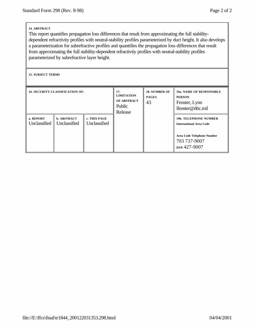
14. ABSTRACT
This report quantifies propagation loss differences that result from approximating the full stability-dependent refractivity profiles with neutral-stability profiles parameterized by duct height. It also develops a parameterization for subrefractive profiles and quantifies the propagation loss differences that result from approximating the full stability-dependent refractivity profiles with neutral-stability profiles parameterized by subrefractive layer height.
15. SUBJECT TERMS
16. SECURITY CLASSIFICATION OF: 17. LIMITATION
OF ABSTRACT
Public Release
18. NUMBER OF
PAGES
43
19a. NAME OF RESPONSIBLE
PERSON
Fenster, Lynn [email protected]
a. REPORT
Unclassifiedb. ABSTRACT
Unclassifiedc. THIS PAGE
Unclassified19b. TELEPHONE NUMBER
International Area Code
Area Code Telephone Number
703 737-9007 DSN 427-9007

SSC SAN DIEGOSan Diego, California 92152--5001
Ernest L. Valdes, CAPT, USN R. C. KolbCommanding Officer Executive Director
SB
ADMINISTRATIVE INFORMATION
The work described in this report was prepared for the Office of Naval Research (ONR 322) bythe SSC San Diego Atmospheric Propagation Branch (D858).
Released byR. A. Paulus, HeadAtmospheric Propagation Branch
Under authority ofC. J. Sayre, HeadElectromagnetics &Advanced TechnologyDivision
iii
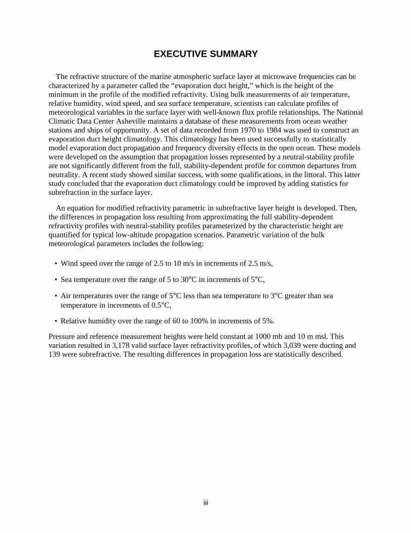
EXECUTIVE SUMMARY
The refractive structure of the marine atmospheric surface layer at microwave frequencies can becharacterized by a parameter called the “evaporation duct height,” which is the height of theminimum in the profile of the modified refractivity. Using bulk measurements of air temperature,relative humidity, wind speed, and sea surface temperature, scientists can calculate profiles ofmeteorological variables in the surface layer with well-known flux profile relationships. The NationalClimatic Data Center Asheville maintains a database of these measurements from ocean weatherstations and ships of opportunity. A set of data recorded from 1970 to 1984 was used to construct anevaporation duct height climatology. This climatology has been used successfully to statisticallymodel evaporation duct propagation and frequency diversity effects in the open ocean. These modelswere developed on the assumption that propagation losses represented by a neutral-stability profileare not significantly different from the full, stability-dependent profile for common departures fromneutrality. A recent study showed similar success, with some qualifications, in the littoral. This latterstudy concluded that the evaporation duct climatology could be improved by adding statistics forsubrefraction in the surface layer.
An equation for modified refractivity parametric in subrefractive layer height is developed. Then,the differences in propagation loss resulting from approximating the full stability-dependentrefractivity profiles with neutral-stability profiles parameterized by the characteristic height arequantified for typical low-altitude propagation scenarios. Parametric variation of the bulkmeteorological parameters includes the following:
• Wind speed over the range of 2.5 to 10 m/s in increments of 2.5 m/s,
• Sea temperature over the range of 5 to 30°C in increments of 5°C,
• Air temperatures over the range of 5°C less than sea temperature to 3°C greater than seatemperature in increments of 0.5°C,
• Relative humidity over the range of 60 to 100% in increments of 5%.
Pressure and reference measurement heights were held constant at 1000 mb and 10 m msl. Thisvariation resulted in 3,178 valid surface layer refractivity profiles, of which 3,039 were ducting and139 were subrefractive. The resulting differences in propagation loss are statistically described.


v
CONTENTSEXECUTIVE SUMMARY ......................................................................................................... iii
INTRODUCTION.......................................................................................................................1
BACKGROUND..................................................................................................................... 1
DATA AND MODELS ...............................................................................................................3
REFRACTIVITY CHARACTERIZATION ...............................................................................3SURFACE LAYER MODEL...................................................................................................5METEOROLOGICAL PARAMETERS...................................................................................6PROPAGATION MODELING ..............................................................................................10
RESULTS................................................................................................................................13
STATISTICS........................................................................................................................13OBSERVATIONS ................................................................................................................17
CONCLUSIONS......................................................................................................................31
REFERENCES........................................................................................................................33
Figures 1. Statistics and histogram for computed evaporation duct heights. Histogram is in 1-m bins...82. Comparison of the simulated evaporation duct height distributions calculated using the
Frederickson et al. (2000) model and the Jeske Paulus (Paulus, 1989) model with 2-m bin size............................................................................................................................9
3. Evaporation duct height versus the stability parameter, z/L ...................................................94. Propagation loss (PL) versus range at 5-m altitude for 3 and 5 GHz (top and bottom
graph, respectively) transmitters at 15 m. Numbers associated with the vertical bars show minimum, standard atmosphere, and maximum PL at 10, 25, and 40 km .................11
5. Propagation loss (PL) versus range at 5-m altitude for 9 and 18 GHz (top and bottom graph, respectively) transmitters at 15 m. Numbers associated with the vertical bars show minimum, standard atmosphere, and maximum PL at 10, 25, and 40 km for 9 GHz and 10 and 25 km for 18 GHz...................................................................................12
6. Histogram of differences between propagation loss for stability-dependent profiles (PL) and propagation loss for neutral profiles (PLN) at 3 GHz and ranges of 10 km (top), 25 km (middle), and 40 km (bottom) ....................................................................................14
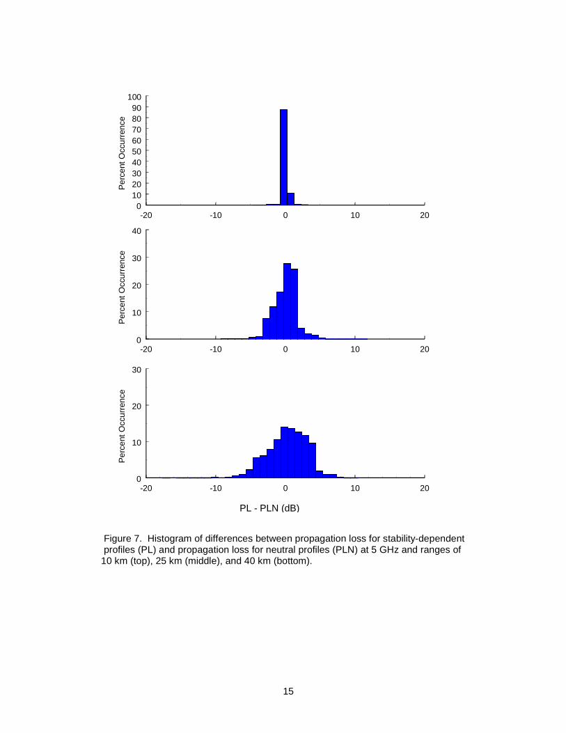
7. Histogram of differences between propagation loss for stability-dependent profiles (PL) and propagation loss for neutral profiles (PLN) at 5 GHz and ranges of 10 km (top), 25 km (middle), and 40 km (bottom) ....................................................................................15
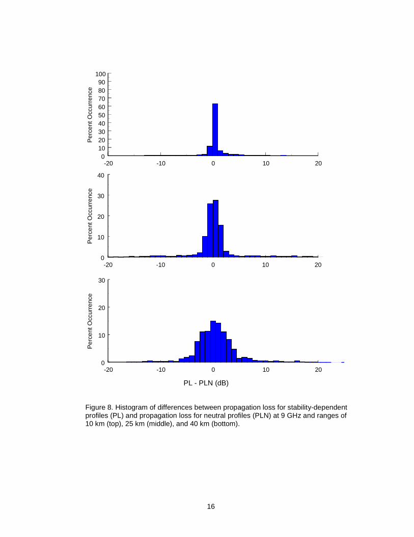
8. Histogram of differences between propagation loss for stability-dependent profiles (PL) and propagation loss for neutral profiles (PLN) at 9 GHz and ranges of 10 km (top), 25 km (middle), and 40 km (bottom) ....................................................................................16
9. Histogram of differences between propagation loss for stability-dependent profiles (PL) and propagation loss for neutral profiles (PLN) at 18 GHz and ranges of 10 km (top) and 25 km (bottom)..............................................................................................................17

vi
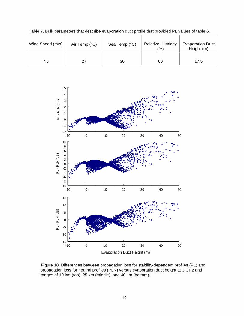
10. Differences between propagation loss for stability-dependent profiles (PL) and propagation loss for neutral profiles (PLN) versus evaporation duct height at 3 GHz and ranges of 10 km (top), 25 km (middle), and 40 km (bottom).........................................19
11. Differences between propagation loss for stability-dependent profiles (PL) and propagation loss for neutral profiles (PLN) versus evaporation duct height at 5 GHz and ranges of 10 km (top), 25 km (middle), and 40 km (bottom).........................................20
12. Differences between propagation loss for stability-dependent profiles (PL) and propagation loss for neutral profiles (PLN) versus evaporation duct height at 9 GHz and ranges of 10 km (top), 25 km (middle), and 40 km (bottom).........................................21
13. Differences between propagation loss for stability-dependent profiles (PL) and propagation loss for neutral profiles (PLN) versus evaporation duct height at 18 GHz and ranges of 10 km (top) and 25 km (bottom)....................................................................22
14. Overplot of propagation loss for stability-dependent profiles and propagation loss for neutral profiles versus evaporation duct height at 3 GHz and ranges of 10 km (top), 25 km (middle), and 40 km (bottom) ....................................................................................23
15. Overplot of propagation loss for stability-dependent profiles and propagation loss for neutral profiles versus evaporation duct height at 5 GHz and ranges of 10 km (top), 25 km (middle), and 40 km (bottom) ....................................................................................24
16. Overplot of propagation loss for stability-dependent profiles and propagation loss for neutral profiles versus evaporation duct height at 9 GHz and ranges of 10 km (top), 25 km (middle), and 40 km (bottom) ....................................................................................25
17. Overplot of propagation loss for stability-dependent profiles and propagation loss for neutral profiles versus evaporation duct height at 18 GHz and ranges of 10 km (top) and 25 km (bottom)..............................................................................................................26
18. Differences between propagation loss for stability dependent profiles (PL) and propagation loss for neutral profiles (PLN) versus the stability parameter, z/L, at 3 GHz and ranges of 10 km (top), 25 km (middle), and 40 km (bottom)..............................27
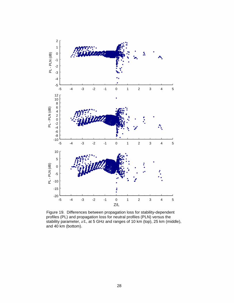
19. Differences between propagation loss for stability-dependent profiles (PL) and propagation loss for neutral profiles (PLN) versus the stability parameter, z/L, at 5 GHz and ranges of 10 km (top), 25 km (middle), and 40 km (bottom)..............................28
20. Differences between propagation loss for stability-dependent profiles (PL) and propagation loss for neutral profiles (PLN) versus the stability parameter, z/L, at 9 GHz and ranges of 10 km (top), 25 km (middle), and 40 km (bottom)..............................29
21. Differences between propagation loss for stability-dependent profiles (PL) and propagation loss for neutral profiles (PLN) versus the stability parameter, z/L, at 18 GHz and ranges of 10 km (top) and 25 km.....................................................................30
Tables 1. Surface layer model input parameter limits............................................................................5 2. Bulk parameter variations ...................................................................................................... 6 3. Description of z/L with respect to wind speed and air–sea temperature difference (ASTD).. 7 4. Statistics of propagation loss (PL) differences between PL from stability-dependent profiles and PL from neutral profiles .................................................................................... 13 5. Estimated neutral evaporation duct and subrefractive layer height at which multi-mode propagation begins to be significant at a given frequency................................................... 18 6. Propagation loss from stability-dependent profile (PL), neutral profile (PLN), and the difference (PL-PLN) versus frequency................................................................................. 18 7. Bulk parameters that describe evaporation duct profile that provided PL values of table 6 .................................................................................................................................. 19

1
INTRODUCTION
This report quantifies propagation loss differences that result from approximating the full stability-dependent refractivity profiles with neutral-stability profiles parameterized by duct height. It alsodevelops a parameterization for subrefractive profiles and quantifies the propagation loss differencesthat result from approximating the full stability-dependent refractivity profiles with neutral-stabilityprofiles parameterized by subrefractive layer height.
BACKGROUND
The refractive structure of the marine atmospheric surface layer at microwave frequencies can becharacterized by a parameter called the “evaporation duct height,” which is the height of theminimum in the profile of the modified refractivity. Using bulk measurements of air temperature,relative humidity, wind speed, and sea surface temperature, scientists can calculate profiles ofmeteorological variables in the surface layer with well-known flux profile relationships. TheNational Climatic Data Center Asheville maintains a database of these measurements from oceanweather stations and ships of opportunity. A set of data recorded from 1970 to 1984 was used toconstruct an evaporation duct height climatology (Anderson, 1987; Patterson, 1987). The evaporationduct height can be used to reconstruct a modified refractivty profile and applied to propagationproblems under the assumption that the propagation losses represented by a neutral-stability profileare not significantly different from the full stability-dependent profile for common departures fromneutrality. The evaporation duct height climatology has been used successfully to statistically modelevaporation duct propagation (Hitney and Vieth, 1990) and frequency diversity effects (Hitney andHitney, 1990) in the open ocean and, with some qualification, in the littoral (Paulus and Anderson,2000). Paulus and Anderson (2000) concluded that the evaporation duct climatology could beimproved by adding statistics for subrefraction in the surface layer.
The DATA AND MODELS section reviews the development of the equation for modified refrac-tivity parametric in duct height for neutral stability and extends this parameterization to account forsubrefraction by subrefractive layer height and “negative evaporation duct height.” The model of themarine atmospheric surface layer is described and the parametric variations of the surface layermodel input data are defined. The electromagnetic propagation model is described and the propaga-tion model output data selected for analysis are defined. The RESULTS section presents the statisticsand case studies. The CONCLUSIONS section summarizes the findings of this work.


3
DATA AND MODELS
REFRACTIVITY CHARACTERIZATION
The refractive index, n, of the atmosphere is often expressed in terms of refractivity, N = (n-1) ×106, or modified refractivity, M = N + 0.157z, where z is height in meters. Refractivity can bemeasured directly with a refractometer or derived from measurements of pressure, P (mb),temperature, T (K), and water vapor pressure, e (mb), using
251073.3
6.77
T
e
T
PN ×+= . (1)
Refractivity is normally a decreasing function with altitude whereas modified refractivity isnormally an increasing function with altitude.
In parametric studies of evaporation duct propagation, it is convenient to have an equation forthe modified refractivity profile as a function of height and evaporation duct height. In theatmospheric surface layer, potential refractivity,
250 1073.3
6.77
θθp
p
ePN ×+= , (2)
is a convenient parameter because of its conservative property in a dynamic atmosphere. Here, θ ispotential temperature (°K), ep is potential water vapor pressure (mb), and P0 is a reference pressurelevel (taken to be 1000 mb). Panofsky and Dutton (1984) provide a general expression for thegradient of a conservative scalar in the atmospheric surface layer which, for potential refractivity,becomes
=
∂∂
L
z
z
N
z
N pp φκ
* , (3)
where z is altitude, Np* is the potential refractivity scaling parameter, κ is von Karman’s constant, ϕis a stability function, and L is the Monin Obukhov stability length. For neutral stability, ϕ is 1 andintegrating equation (3) from a lower limit of z0 yields
( ) ( )0
*0 ln
z
zNzNzN p
pp κ=− , (4)
where the aerodynamic roughness length, z0, is taken to be 1.5 x 10⁻⁴ m.
From geometric optics, the critical gradient required for trapping is that which yields a ray curva-ture equal to the earth’s curvature (Bean and Dutton, 1968):
157.0106
−=−=adz
dN N/m, (5)

4
where a is the earth radius in meters. In terms of modified refractivity, the critical gradient is
0=dz
dM. (6)
That is, the evaporation duct height is the top of the surface trapping layer. Gossard and Strauch(1983) relate Np to N and M by
zNN p 024.0+= and (7)
zMN p 13.0−= (8)
so that dNp/dz = -0.13 for trapping. Defining the height at which this critical gradient occurs as theevaporation duct height, δ, equation (3) becomes
κδ
*13.0 pN=− . (9)
Solving equation (4) for Np*, substituting in equation (9), and using the relation of equation (8)
yields
−+=
00 ln13.013.0)(
z
zzMzM δ , (10)
where M0, the value of modified refractivity at the sea surface temperature assuming saturation,approximates M(z0). Similarly, it would be convenient to have an equation for the modifiedrefractivity profile as a function of height and some parameterization of subrefraction. Similar to theheight of the evaporation duct being the top of a surface trapping layer where dM/dz = 0, there is aheight that is the top of a surface subrefractive layer where dN/dz = 0. Defining the height at whichthis critical gradient occurs as the subrefractive layer height, ς , dNp/dz = 0.024 and equation (9)becomes
κς*024.0 pN
= . (11)
Again, solving equation (4) for Np*, substituting in equation (11), and using the relation of equation
(8) yields
++=
00 ln024.013.0)(
z
zzMzM ς . (12)

5
Equations (10) and (12) can generate ducting and subrefractive profiles parametric in evaporationduct height and subrefractive layer height, respectively. Jeske (1973) referred to subrefraction as an“anti-duct.” In his formulation, subrefractive conditions produced a negative duct height. While anegative duct height is not physically realistic, that parameter does allow one to analyze results of allrefractive conditions versus one parameter. Simultaneous solution of equations (10) and (12)produces
ςδ 185.0−= , (13)
which can be used to present results against whichever parameterization is more convenient. Forinput to the propagation model, the modified refractivity profile was digitized at discrete heights inmeters according to
xez = , (14)
where x = -2 to 5 in 0.5 increments, i.e., 0.1354 to 148.4132 m.
SURFACE LAYER MODEL
The surface layer model developed by Frederickson, Davidson, and Goroch (2000) was used forthis study. Model input requirements are wind speed (m/s), air temperature (°C), sea surfacetemperature (°C), relative humidity (%), atmospheric pressure (mb), and the heights of measurementof the four atmospheric parameters (m msl). Table 1 shows valid values of these input parameters.Model outputs are the evaporation duct height (0 to 50 m) and the profile of modified refractivityfrom the sea surface to 50 m msl. In some very stable cases, the model algorithm will not convergeand there is no valid solution for some combinations of input data.
Table 1. Surface layer model input parameter limits.
Parameter Inclusive Limits
Wind speed 1 to 40 m/s
Air temperature -55 to 55°C
Sea surface temperature -2 to 40°C
Relative humidity 0 to 101%
Atmospheric pressure 940 to 1040 mb
Measurement height 1 to 50 m

6
For our purposes, refractivity profiles, N(z), were computed along with the modifiedrefractivity profiles for the subrefractive conditions. The height of the maximum value ofrefractivity was selected as the subrefractive layer height. For the comparisons in this report, weused only evaporation duct heights and subrefractive layer heights <50 m. The Monin–Obukhovlength, L, was also extracted from the surface layer model to generate the stability parameter,z/L.
METEOROLOGICAL PARAMETERS
The variation of the bulk parameters was arbitrarily selected to be typical ocean conditions byexamination of the climatological data from the Marine Climatic Atlas of the World series (U.S.Navy, 1974). The data presented in the climatology are independent. There is no information as tothe joint occurrence probability of any combination of the meteorological parameters. Here, we haveassumed each combination of bulk parameters is equally probable. Table 2 shows the input datarange and the increment used for iteration. This combination produces a potential for 3,672 differentenvironmental conditions. However, 281 conditions had evaporation duct heights equal to or greaterthan 50 m, 209 had subrefractive layer heights equal to or greater than 50 m, and in four cases, thesurface layer algorithm did not converge to a result. Thus, there were 3,178 environments for whichpropagation loss could be calculated. Of these, 3,039 (96%) were ducting conditions and 139 weresubrefractive (4%) conditions. Of the ducting conditions, 635 were stable ducts (20%) and 2,404were unstable ducts (76%)
Table 2. Bulk parameter variations.
Parameter Inclusive Limits Increment
Wind speed 2.5 to 10 m/s 2.5 m/s
Air temperature Sea - 5 to Sea +3°C 0.5°C
Sea surface temperature 5 to 30°C 5°C
Relative humidity 60 to 100% 5%
Atmospheric pressure 1000 mb None
Measurement height 10 m None

7
Figure 1 shows the statistics and histogram for the simulated evaporation duct heights. This figureindicates good coverage of duct heights for the simulated data. Figure 2 shows the distribution ofsimulated duct heights (positive duct heights only) calculated with the Frederickson et al. (2000)model plotted with the distribution of duct heights calculated using the current standard evaporationduct model (Paulus, 1989) for the same parametric data set. The shapes of the two distributions aresimilar except that the Frederickson distribution has a lower mean (9.27 m compared to 10.8 m) andgreater kurtosis. Figure 3 shows evaporation duct height versus the z/L stability parameter thatFrederickson et al. (2000) define as
2*
*
u
gz
L
z
v
v
θθκ
= . (15)
Here, θv is virtual potential temperature, θ* v is the virtual potential temperature scaling parameter,
and u* is the scaling parameter for momentum. Physically, z/L is the ratio of turbulent kinetic energygenerated by thermal buoyancy to turbulent kinetic energy generated by wind shear. Table 3 shows aqualitative description of z/L based on Panofsky and Dutton (1984). A wide range of stability occursin the simulated data, with most (72%) in the range, |z/L| < 0.5. This range is approximately the near-neutral Pasquill–Gifford stability category D (Hsu, 1992). Notice from figure 3 that all negative ductheights (subrefractive layers) occur under stable conditions and mostly near neutral. The largest ductheights also occur under stable conditions and mostly near neutral. It is operationally significant thatthe greatest variation in duct heights occurs near neutral. Blanc (1987) showed that near neutral is theregion in which it is most difficult to accurately determine stability using bulk measurements. Thus,errors in determining the evaporation duct characteristics are likely greatest near neutral.
Table 3. Description of z/L with respect to wind speed and air–sea temperature difference (ASTD).
Value of z/L Description Physical Meaning
Strongly negative (z/L < -0.5) Unstable Thermal convection dominant; lighterwinds or large, negative ASTD
Negative, but small (-0.5 < z/L <0)
Unstable, nearneutral
Mechanical turbulence dominant;higher winds or small, negative ASTD
Zero Neutral Purely mechanical turbulence
Slightly positive (0 < z/L < 0.5) Stable, nearneutral
Mechanical turbulence slightly dampedby thermal stratification; higher windsor small, positive ASTD
Strongly positive (z/L > 0.5) Stable Mechanical turbulence severelyreduced by thermal stratification; lighterwinds or large, positive ASTD

8
Minimum duct height (m) -9.2
Maximum duct height (m) 49.4
Mean 8.76
Median 7.00
Variance 57.94
Standard Deviation 7.61
Total Observations 3178
-10 0 10 20 30 40 50
Evaporation Duct Height (m)
0
1
2
3
4
5
6
7
8
9
10
Per
cent
Occ
urre
nce
Figure 1. Statistics and histogram for computed evaporation duct heights. Histogram is in 1-m bins.

9
-5 -4 -3 -2 -1 0 1 2 3 4 5
Z/L
-10
0
10
20
30
40
50
Eva
pora
tion
Duc
t Hei
ght (
m)
Figure 3. Evaporation duct height versus the stability parameter, z/L.
0
5
10
15
20
0 2 4 6 8 10 12 14 16 18 20 22 24 26 28 30 32 34 36 38 40Evaporation Duct Height (m)
Per
cent
Occ
urre
nce
Frederickson et al.
Jeske Paulus
Figure 2. Comparison of the simulated evaporation duct height distributions calculated usingthe Frederickson et al. (2000) model and the Jeske Paulus (Paulus, 1989) model with 2-m binsize.

10
PROPAGATION MODELING
The propagation model used in this study was the hybrid ray-optics/parabolic equation RadioPhysical Optics (RPO) model (Hitney, 1992). RPO can partially account for sea surface roughness byassuming a fully arisen sea for the given wind speed. However, for this study, the sea surface wasassumed flat, and molecular absorption was neglected. The propagation scenarios selected used ahorizontally polarized transmitter at 15 m msl with a 2° wide Gaussian beam at 0° elevation.Propagation loss values were calculated for a receiver located at 5 m msl at frequencies of 3, 5, and9 GHz at ranges of 10, 25, and 40 km and for 18 GHz at 10 and 25 km. The 25-km range is approxi-mately at the 4/3 earth radio horizon and the 10-km range lies well within the horizon. The 40-kmrange was selected such that troposcatter was not a factor in the standard atmosphere (4/3 earthradius) propagation loss. Propagation loss was calculated using the 3,178 full stability-dependentrefractivity profiles and the neutral profiles using the same duct or subrefractive layer height inequation (10) or (12). The solid line in figures 4 and 5 shows standard atmosphere propagation loss ata 5-m altitude for each of the four frequencies. The vertical lines in each plot indicate the variation inpropagation loss over the 3,178 profiles at each range. At 3 and 5 GHz (figure 4), evaporationducting causes signal levels to be near or above standard. Subrefraction causes signal levels to bebelow standard. At 9 GHz (top graph, figure 5), evaporation ducting causes signal levels to be near orabove standard at 25 and 40 km, but subrefraction and evaporation ducting reduce signal levelsbelow standard at 10 km. Evaporation ducting causes the maximum modeled propagation loss of141.5 dB at 10 km and subrefraction causes the maximum losses of 184.5 dB and 211.1 dB at 25 and40 km, respectively. Evaporation ducting causing greater propagation loss within the horizon wasexpected, as it has been modeled (Dockery, 1987) and measured (Anderson, 1995) previously.Likewise, the propagation effects at 18 GHz (bottom graph, figure 5) are similar to those at 9 GHz.

11
0 1 0 2 0 3 0 4 0 5 0
R a n g e ( k m )
2 0 0
1 8 0
1 6 0
1 4 0
1 2 0
1 0 0
8 0
Pro
pa
ga
tio
n L
os
s (
dB
)1 1 7 .61 2 5 .2
1 2 7 .4
1 2 3 .4
1 5 0 .5
1 5 9 .7
1 2 4 .9
1 7 2 .2
1 8 9 .7
0 1 0 2 0 3 0 4 0 5 0R a n g e
2 0 0
1 9 0
1 8 0
1 7 0
1 6 0
1 5 0
1 4 0
1 3 0
1 2 0
1 1 0
1 0 0
Pro
pL
os
s
1 2 0 .3
1 2 5 .2
1 2 8 .5
1 2 8 .1
1 5 0 .5
1 6 6 .1
1 2 9 .0
1 7 2 .2
1 9 7 .2
Figure 4. Propagation loss (PL) versus range at 5-m altitude for 3 and 5 GHz (topand bottom graph, respectively) transmitters at 15 m. Numbers associated with thevertical bars show minimum, standard atmosphere, and maximum PL at 10, 25,and 40 km.

12
0 1 0 2 0 3 0 4 0 5 0
R a n g e ( k m )
2 2 0
2 0 0
1 8 0
1 6 0
1 4 0
1 2 0
1 0 0
Pro
pa
ga
tio
n L
os
s (
dB
) 1 2 5 .81 2 7 .3
1 4 1 .5
1 3 3 .5
1 5 6 .4
1 8 4 .5
1 3 6 .1
1 8 6 .6
2 1 1 .1
0 1 0 2 0 3 0 4 0 5 0
R a n g e ( k m )
2 2 0
2 0 0
1 8 0
1 6 0
1 4 0
1 2 0
1 0 0
Pro
pa
ga
tio
n L
os
s (
dB
)
1 3 1 .5
1 3 3 .2
1 5 6 .2
1 4 0 .6
1 6 0 .6
1 9 3 .0
Figure 5. Propagation loss (PL) versus range at 5-m altitude for 9 and 18 GHz (topand bottom graph, respectively) transmitters at 15 m. Numbers associated with thevertical bars show minimum, standard atmosphere, and maximum PL at 10, 25, and 40km for 9 GHz and 10 and 25 km for 18 GHz.

13
RESULTS
STATISTICS
For the scenarios of the four frequencies and the multiple ranges, the difference betweenpropagation loss determined for the full stability-dependent modified refractivity profiles andpropagation loss determined for the neutral-stability modified refractivity profiles was calculated.Figures 6 through 9 show histograms of the differences. The difference distributions tend to beskewed at 3 and 5 GHz, but symmetric at 9 and 18 GHz. All distributions are sharply peaked and themean differences are near zero. Table 4 shows the descriptive statistics of the distributions for thefour frequencies and multiple ranges. The mean propagation loss (PL) differences are small and thestandard deviations of the differences are on the order of a few dB, indicating that the neutral profileestimate is reasonably good.
Table 4. Statistics of propagation loss (PL) differences between PL from stability-dependentprofiles and PL from neutral profiles.
Frequency Range
LargestNegative
PLDifference
(dB)
LargestPositive
PLDifference
(dB)
Mean PLDifference
(dB)
Median PLDifference
(dB)
StandardDeviation of
PLDifferences
(dB)
10 km -1.7 4.4 0.04 0.00 0.64
25 km -6.4 9.5 0.30 0.40 1.733 GHz
40 km -12.7 12.3 0.52 1.00 2.85
10 km -4.7 1.7 -0.07 0.00 0.43
25 km -9.2 10.4 -0.03 0.10 1.675 GHz
40 km -17.6 8.4 0.26 0.40 2.86
10 km -13.1 12.8 0.24 0.10 2.74
25 km -24.2 21.9 0.14 0.10 4.649 GHz
40 km -16.5 27.7 0.32 0.20 3.91
10 km -17.0 18.7 -0.73 -0.10 4.8418 GHz
25 km -18.9 19.2 0.31 0.40 4.66

14
-20 -10 0 10 200
102030405060708090
100
Per
cent
Occ
urre
nce
-20 -10 0 10 200
10
20
30
40
Per
cent
Occ
urre
nce
-20 -10 0 10 20
PL - PLN (dB)
0
10
20
30
Per
cent
Occ
urre
nce
Figure 6. Histogram of differences between propagation loss for stability-dependent profiles (PL)and propagation loss for neutral profiles (PLN) at 3 GHz and ranges of 10 km (top), 25 km(middle), and 40 km (bottom).
15
-20 -10 0 10 200
102030405060708090
100
Per
cent
Occ
urre
nce
-20 -10 0 10 200
10
20
30
40
Per
cent
Occ
urre
nce
-20 -10 0 10 20
PL - PLN (dB)
0
10
20
30
Per
cent
Occ
urre
nce
Figure 7. Histogram of differences between propagation loss for stability-dependent profiles (PL) and propagation loss for neutral profiles (PLN) at 5 GHz and ranges of 10 km (top), 25 km (middle), and 40 km (bottom).
16
-20 -10 0 10 200
102030405060708090
100
Per
cent
Occ
urre
nce
-20 -10 0 10 200
10
20
30
40
Per
cent
Occ
urre
nce
-20 -10 0 10 20
PL - PLN (dB)
0
10
20
30
Per
cent
Occ
urre
nce
Figure 8. Histogram of differences between propagation loss for stability-dependent profiles (PL) and propagation loss for neutral profiles (PLN) at 9 GHz and ranges of 10 km (top), 25 km (middle), and 40 km (bottom).

17
OBSERVATIONS
Because the range of variation chosen for the bulk parameters was arbitrary, and there is noclimatological data as to the joint occurrence of any given combination of parameters, it isworthwhile to examine the differences further. Figures 10 through 13 show propagation lossdifferences plotted versus evaporation duct height. The differences are not evenly distributed over therange of evaporation duct height. Differences tend to remain small from approximately -5 m (27-msubrefractive layer height) to approximately 15-m evaporation duct height for 3, 5, and 9 GHz andover a slightly smaller range at 18 GHz. Outside these ranges, differences increase markedly. Viewedanother way, figures 14 through 17 show both PL from stability-dependent profiles and PL fromneutral profiles versus evaporation duct height. At 5, 9, and 18 GHz, the variations in the plot of PLat the higher duct heights show the effects of multiple modes being propagated in the duct. There is awider variation in resulting PL at higher duct heights. The neutral evaporation duct height at whichmulti-mode propagation begins to be significant is a function of frequency and has been previouslyestimated (Patterson et al., 1990) as shown in table 5. The duct heights of table 5 are in reasonablequalitative agreement with the increase in differences between PL from stability-dependent profilesand PL from neutral profiles shown figures 10 through 17. The impact of this increase in differencesis that simulations of propagation effects parametric in evaporation duct height become less represen-
-20 -15 -10 -5 0 5 10 15 200
102030405060708090
100P
erce
nt O
ccur
renc
e
-20 -15 -10 -5 0 5 10 15 20
PL - PLN (dB)
0
10
20
30
40
Per
cent
Occ
urre
nce
Figure 9. Histogram of differences between propagation loss for stability-dependent profiles (PL) and propagation loss for neutral profiles (PLN) at 18 GHz and ranges of 10 km (top) and 25 km (bottom).

18
tative of real propagation effects at higher duct heights. Qualitatively, from figures 10 through 17,this also appears to be true for more negative duct heights (higher subrefractive layers). Table 5 alsoshows approximate subrefractive layer heights above which multi-mode propagation begins to besignificant and simulation using a neutral profile becomes less representative of real propagationeffects.
A consequence of the inverse correlation between frequency and the evaporation duct height atwhich multiple modes become important is that the neutral profile can be a very good approximationto the propagation effects of the full stability-dependent profile at one frequency, but not at another.Table 6 shows such an example for the propagation loss at 10 km. The differences in PL from astability-dependent profile and a neutral profile are small at 3 and 5 GHz, but much larger at 9 and18 GHz.
Table 7 shows the bulk parameters and evaporation duct height for the results in table 6. Theevaporation duct height for this set of bulk parameters is 17.5 m. In table 5, the 17.5-m evaporationduct height falls between the values at 5 GHz and 10 GHz. This height would indicate that3 and 5 GHz should be dominated by single-mode propagation and that 9 and 18 GHz should beaffected by multiple modes propagating in the duct. Thus, we should expect that the neutral profilewould be a good approximation of the stability-dependent profile propagation loss at the two lowerfrequencies, but not as good at the two higher frequencies.
Table 6. Propagation loss from stability- dependent profile (PL), neutral profile (PLN),
and the difference (PL-PLN) versus frequency.
Frequency(GHz)
PL(dB)
PLN(dB)
PLDifference
(dB)
3 119.6 120.9 -1.3
5 121.1 121.6 -0.5
9 141.5 128.7 12.8
18 143.4 132.1 11.3
Table 5. Estimated neutral evaporation duct and subrefractive layer height at which multi-mode propagation begins to be significant at a given frequency.
Frequency(GHz)
Neutral Evaporation DuctHeight (m)
Neutral Subrefractive LayerHeight (m)
3 30 40
5 22 27
10 14 16
18 10 10
19
Table 7. Bulk parameters that describe evaporation duct profile that provided PL values of table 6.
Wind Speed (m/s) Air Temp (°C) Sea Temp (°C) Relative Humidity(%)
Evaporation DuctHeight (m)
7.5 27 30 60 17.5
-10 0 10 20 30 40 50-2
-1
0
1
2
3
4
5
PL
- P
LN (
dB)
-10 0 10 20 30 40 50-10-8-6-4-202468
10
PL
- P
LN (
dB)
-10 0 10 20 30 40 50
Evaporation Duct Height (m)
-15
-10
-5
0
5
10
15
PL
- P
LN (
dB)
Figure 10. Differences between propagation loss for stability-dependent profiles (PL) and propagation loss for neutral profiles (PLN) versus evaporation duct height at 3 GHz and ranges of 10 km (top), 25 km (middle), and 40 km (bottom).

20
-10 0 10 20 30 40 50-5-4-3-2-1012345
PL
- P
LN (
dB)
-10 0 10 20 30 40 50-10-8-6-4-202468
10
PL
- P
LN (
dB)
-10 0 10 20 30 40 50
Evaporation Duct Height (m)
-20
-15
-10
-5
0
5
10
PL
- P
LN (
dB)
Figure 11. Differences between propagation loss for stability-dependent profiles (PL)and propagation loss for neutral profiles (PLN) versus evaporation duct height at5 GHz and ranges of 10 km (top), 25 km (middle), and 40 km (bottom).

21
-10 0 10 20 30 40 50-15
-10
-5
0
5
10
15
PL
- P
LN (
dB)
-10 0 10 20 30 40 50-25
-15
-5
5
15
25
PL
- P
LN (
dB)
-10 0 10 20 30 40 50
Evaporation Duct Height (m)
-20
-10
0
10
20
30
PL
- P
LN (
dB)
Figure 12. Differences between propagation loss for stability-dependent profiles (PL) and propagation loss for neutral profiles (PLN) versus evaporation duct height at 9 GHz and ranges of 10 km (top), 25 km (middle), and 40 km (bottom).

22
-10 0 10 20 30 40 50-20
-10
0
10
20
PL
- P
LN (
dB)
-10 0 10 20 30 40 50
Evaporation Duct Height (m)
-20
-10
0
10
20
PL
- P
LN (
dB)
Figure 13. Differences between propagation loss for stability-dependent profiles (PL) and propagation loss for neutral profiles (PLN) versus evaporation duct height at 18 GHz and ranges of 10 km (top) and 25 km (bottom).

23
-10 0 10 20 30 40 50130
125
120
115
Pro
paga
tion
Loss
(dB
)
-10 0 10 20 30 40 50170
160
150
140
130
120
Pro
paga
tion
Loss
(dB
)
-10 0 10 20 30 40 50
Evaporation Duct Height (m)
200
190
180
170
160
150
140
130
120
Pro
paga
tion
Loss
(dB
)
PL (dB) from Stability Dependent ProfilesPL (dB) from Neutral Profiles
Figure 14. Overplot of propagation loss for stability-dependent profiles and propagation loss for neutral profiles versus evaporation duct height at 3 GHz and ranges of 10 km (top), 25 km (middle), and 40 km (bottom).

24
-10 0 10 20 30 40 50130
128
126
124
122
120
Pro
paga
tion
Loss
(dB
)
-10 0 10 20 30 40 50170
160
150
140
130
120
Pro
paga
tion
Loss
(dB
)
-10 0 10 20 30 40 50
Evaporation Duct Height (m)
200
190
180
170
160
150
140
130
120
Pro
paga
tion
Loss
(dB
)
PL (dB) from Stability Dependent ProfilesPL (dB) from Neutral Profiles
Figure 15. Overplot of propagation loss for stability-dependent profiles and propagation loss for neutral profiles versus evaporation duct height at 5 GHz and ranges of 10 km (top), 25 km (middle), and 40 km (bottom).

25
-10 0 10 20 30 40 50150
145
140
135
130
125
120
Pro
paga
tion
Loss
(dB
)
-10 0 10 20 30 40 50190
180
170
160
150
140
130
Pro
paga
tion
Loss
(dB
)
-10 0 10 20 30 40 50
Evaporation Duct Height (m)
220
205
190
175
160
145
130
Pro
paga
tion
Loss
(dB
)
PL (dB) from Stability Dependent ProfilesPL (dB) from Neutral Profiles
Figure 16. Overplot of propagation loss for stability-dependent profiles and propagation loss for neutral profiles versus evaporation duct height at 9 GHz and ranges of 10 km (top), 25 km (middle), and 40 km (bottom).

26
Figures 18 to 21 show the difference in propagation loss from stability-dependent and neutralmodified refractivity profiles versus the stability parameter, z/L, for the four frequencies and multipleranges. While there are relatively large differences in PL in the unstable and stable regions, most ofthe larger differences occur near neutral. This occurrence is consistent with figure 3, which showedthat the higher duct and subrefractive layer heights occurred near neutral. Therefore, because thehigher duct and subrefractive layer heights support multi-mode propagation, we conclude that thelargest PL differences will also occur in near-neutral conditions.
Note that the propagation effects of a 0-m evaporation duct are not the same as a standardatmosphere. A close comparison of the standard atmosphere PL values from figures 4 and 5 with the0-m duct height values in figures 14 through 17 shows that 0-m evaporation duct PL values may beup to a few dB greater than standard atmosphere, particularly at 25 and 40 km. This increase is theresult of the standard atmosphere gradient being 0.118 M/m versus the 0-m evaporation duct gradientof 0.130 M/m, determined by the derivative of equation (10).
-10 0 10 20 30 40 50160
155
150
145
140
135
130
Pro
paga
tion
Loss
(dB
)
-10 0 10 20 30 40 50Evaporation Duct Height (m)
190
180
170
160
150
140
Pro
paga
tion
Loss
(dB
)
PL (dB) from Stability Dependent ProfilesPL (dB) from Neutral Profiles
Figure 17. Overplot of propagation loss for stability-dependent profiles and propagation loss for neutral profiles versus evaporation duct height at 18 GHz and ranges of 10 km (top) and 25 km (bottom).

27
-5 -4 -3 -2 -1 0 1 2 3 4 5-2
-1
0
1
2
3
4
5
PL
- P
LN (
dB)
-5 -4 -3 -2 -1 0 1 2 3 4 5-10-8-6-4-202468
10
PL
- P
LN (
dB)
-5 -4 -3 -2 -1 0 1 2 3 4 5
Z/L
-15
-10
-5
0
5
10
15
PL
- P
LN (
dB)
Figure 18. Differences between propagation loss for stability dependentprofiles (PL) and propagation loss for neutral profiles (PLN) versus thestability parameter, z/L, at 3 GHz and ranges of 10 km (top), 25 km(middle), and 40 km (bottom).
28
-5 -4 -3 -2 -1 0 1 2 3 4 5-5
-4
-3
-2
-1
0
1
2
PL
- P
LN (
dB)
-5 -4 -3 -2 -1 0 1 2 3 4 5-10-8-6-4-202468
1012
PL
- P
LN (
dB)
-5 -4 -3 -2 -1 0 1 2 3 4 5
Z/L
-20
-15
-10
-5
0
5
10
PL
- P
LN (
dB)
Figure 19. Differences between propagation loss for stability-dependent profiles (PL) and propagation loss for neutral profiles (PLN) versus the stability parameter, z/L, at 5 GHz and ranges of 10 km (top), 25 km (middle), and 40 km (bottom).

29
-5 -4 -3 -2 -1 0 1 2 3 4 5-15
-10
-5
0
5
10
15
PL
- P
LN (
dB)
-5 -4 -3 -2 -1 0 1 2 3 4 5-30
-20
-10
0
10
20
30
PL
- P
LN (
dB)
-5 -4 -3 -2 -1 0 1 2 3 4 5
Z/L
-20
-10
0
10
20
30
PL
- P
LN (
dB)
Figure 20. Differences between propagation loss for stability-dependent profiles (PL) and propagation loss for neutral profiles (PLN) versus the stability parameter, z/L, at 9 GHz and ranges of 10 km (top), 25 km (middle), and 40 km (bottom).

30
-5 -4 -3 -2 -1 0 1 2 3 4 5-20
-10
0
10
20
PL
- P
LN (
dB)
-5 -4 -3 -2 -1 0 1 2 3 4 5
Z/L
-20
-10
0
10
20
PL
- P
LN (
dB)
Figure 21. Differences between propagation loss for stability-dependent profiles (PL) and propagation loss for neutral profiles (PLN) versus the stability parameter, z/L, at 18 GHz and ranges of 10 km (top) and 25 km.

31
CONCLUSIONS
This study finds that subrefractive profiles in the atmospheric surface layer can be parameterizedby a characteristic height similar to the evaporation duct height. This parameter can be in terms ofsubrefractive layer height or negative evaporation duct height. Equation (13) relates the two heights.The parameter “subrefractive layer height” is an easily understood concept and is related to aphysical feature of the refractivity profile. The parameter “negative evaporation duct height” is notrelated to a physical feature of the refractivity profile and evaporation is not the surface layer physi-cal process involved in subrefraction, rather condensation is occurring. However, using a negativeduct height allows plotting of propagation loss predictions versus one parameter demonstrated here.
This study demonstrates that using neutral-stability refractivity profiles, equation (10) or (12),yields a good approximation of the propagation loss resulting from using full stability-dependentprofiles over a typical range of bulk meteorological parameters. The accuracy of this approximationdegrades as the refractive profile supports the propagation of multiple modes, i.e., as the duct heightincreases. This phenomena occurs for higher evaporation duct heights. Table 5 presents the approxi-mate duct heights at which multiple-mode propagation becomes significant.


33
REFERENCES
Anderson, K. D. 1987. “Worldwide Distributions of Shipboard Surface Meteorological Observationsfor EM Propagation Analysis.” NOSC Technical Document 1150 (Sep).Naval Ocean Systems Center*, San Diego, CA.
Anderson, K. D. 1995. “Radar Detection of Low-Altitude Targets in a Maritime Environment.” IEEETransactions on Antennas and Propagation, vol. 43, no. 6 (Jun), pp.609–613.
Bean, B. R. and E. J. Dutton. 1968. Radio Meteorology, Dover Publications, New York, NY.
Blanc, T. V. 1987. “Accuracy of Bulk-Method-Determined Flux, Stability, and Sea Roughness,”Journal of Geophysical Research, vol. 92, no. C4, pp. 3867–3876.
Dockery, G. D. 1987. “Description and Validation of the Electromagnetic Parabolic EquationPropagation Model (EMPE),” FS-87-152 (Sep). Johns Hopkins University/Applied PhysicsLaboratory, Laurel, MD.
Frederickson, P. A., K. L. Davidson, and A. K. Goroch. 2000. “Operational Bulk Evaporation DuctModel for MORIAH,” Draft version 1.2, NPS Report 2000.
Gossard, E. E. and R. G. Strauch. 1983. Radar Observation of Clear Air and Clouds, Elsevier, NewYork, NY.
Hitney, H. V. and R. Vieth. 1990. “Statistical Assessment of Evaporation Duct Propagation,” IEEETransactions on Antennas and Propagation, vol. 38, no. 6 (Jun), pp. 794–799.
Hitney, H. V. and L. R. Hitney. 1990. “Frequency Diversity Effects of Evaporation DuctPropagation,” IEEE Transactions on Antennas and Propagation, vol. 38, no.10 (Oct),pp. 1694–1700.
Hitney, H. V. 1992. “Hybrid Ray Optics and Parabolic Equation Methods for Radar PropagationModeling,” IEE International Conference: RADAR ‘92, Conference Publication No. 365,(pp. 58-61). 12–13 October 1992, Brighton, UK.
Hsu, S. A. 1992. “An Overwater Stability Criterion for the Offshore and Coastal Dispersion Model,”Boundary Layer Meteorology, vol. 50, pp. 397–402.
Jeske, H. 1973. “State and Limits of Prediction Methods of Radar Wave Propagation ConditionsOver Sea.” In Modern Topics in Microwave Propagation and Air–Sea Interaction,p. 131–148, A. Zancla, Ed. Reidel Publishers, Boston, MA.
Panofsky, H. A. and J. A. Dutton. 1984. Atmospheric Turbulence: Models and Methods forEngineering Applications. Wiley, New York, NY.
Patterson, W. L. 1987. “Historical Electromagnetic Propagation Condition Database Description,”NOSC* Technical Document 1149 (Sep). Naval Ocean Systems Center, San Diego, CA.
* now SSC San Diego

34
Patterson, W. L., C. P. Hattan, H. V. Hitney, R. A. Paulus, A. E. Barrios, G. E. Lindem, andK. D. Anderson. 1990. “Engineer’s Refractive Effects Prediction System (EREPS) Revision 2.0.”NOSC* Technical Document 1342 (Feb), Naval Ocean Systems Center, San Diego, CA.
Paulus, R. A. 1989. “Specification for Evaporation Duct Height Calculations,” NOSC* TechnicalDocument 1596 (Jul), Naval Ocean Systems Center, San Diego, CA.
Paulus, R. A. and K. D. Anderson. 2000. “Application Of An Evaporation Duct Climatology in theLittoral,” Proceedings of Battlespace Atmospheric and Cloud Impact on Military Operations(BACIMO) 2000 Conference, 25–27 April, Ft. Collins, CO.
U.S. Navy. 1974. U.S. Navy Marine Climatic Atlas of the World, series, Commander, Naval WeatherService Command, U.S. Government Printing Office, Washington, D.C.
* now SSC San Diego

REPORT DOCUM ENTATION PAGEForm Ap proved
O M B N o . 0704 -01 -0188
T h e pu b lic rep o rting b u rde n for th is co lle ct io n o f info rm a ti on i s e st im ated to ave ra ge 1 h o ur pe r res po ns e, i nc lud in g th e tim e fo r rev iew in g in st ruc ti on s , s e a rch ing e x is ting d ata so u rc e s,g a the rin g an d m a in ta in ing th e da ta n e ed ed , an d co m p le ting a nd re v ie w ing the co lle c tio n of in fo rm atio n . S en d co m m en ts reg a rd ing thi s b urd en e st im a te o r a n y o th er as pe ct o f th is c o lle ct io no f in fo rm a tion , in c lud in g sug g est io n s fo r re du cin g the b u rde n to De p artm e n t of D e fe n s e, W a sh ing to n H e ad qu a rte rs S erv ice s D ire c to ra te for In fo rm at io n O p era t ion s an d R ep o rts(0 70 4-0 1 88 ), 1 21 5 J effe rso n D avis H igh w ay, S u ite 1 20 4 , Arl ing ton VA 2 2 20 2-4 3 02 . R e spo n de nts sh ou ld be aw ar e tha t n o tw ithsta nd in g a ny o th e r p ro v is ion of law , n o p ers on sha ll b e
PLEASE DO NO T RETUR N YO UR FO RM TO THE ABOVE ADDRES S.1. REPO RT DATE (D D -M M -YY YY) 2. RE PO RT TYPE 3. DATE S CO VE RED (F rom - To )
4. TITLE AND S UBTITLE 5a. CONTRACT NUM BER
5b. G RA NT NUMB ER
5c. PRO GRAM ELEM ENT NUM BER
5d. P ROJE CT NUM BER
5e. TASK NUM BER
5f. W ORK UNIT NUM BER
6. AUTHO RS
7. PERFO RM ING ORG AN IZATION NAM E(S) AND ADDRE SS(ES ) 8. PERFO RM ING ORG AN IZATION REPO RT NUM BER
10. SPO NSO R/MO NITOR ’S ACR ON YM (S)
11. SPONS OR /M ONITO R’S R EPO RT NUM BER(S)
9. SPO NSO RING /M ONITO RING AGENCY NAM E(S) AND ADDRESS(ES)
12. DISTRIBUTIO N/AVAILABILITY STATEM EN T
13. SUPPLEM ENTARY N OTES
14. ABSTRA CT
15. SUBJECT TERM S
16. SECURITY CLASSIFIC ATIO N O F:a. REPO RT b. ABSTRACT c. TH IS PAG E
17. LIM ITATION OF AB STRACT
18. NUM BER O F PAG ES
19a . NAM E OF RESPO NSIBLE PERSON
19B. TELEPHO NE NUM BER (Inc lude area code)
Standard Form 298 (R ev. 8 /98)P rescribed by A NSI S td . Z39.18
su b ject to an y p e na lty fo r fa iling to com ply w ith a c o l lec tio n o f in fo rm a tion if it d oe s n o t d is p la y a cu rre n t ly va l id O M B c o ntro l n um b er.
11-2000 Technical
PARMETRIC STUDY OF PROPAGATION IN EVAPORATIONDUCTING AND SUBREFRACTIVE CONDITIONS
PE0602435N
DN302216
R. A. Paulus
MPB3
SSC San DiegoSan Diego, CA 92152-5001 TR 1844
ONROffice of Naval Research (ONR 322)800 North Quincy StreetArlington, VA 22217-5660
Distribution is unlimited; public release
This report quantifies propagation loss differences that result from approximating the full stability-dependent refractivity profileswith neutral-stability profiles parameterized by duct height. It also develops a parameterization for subrefractive profiles andquantifies the propagation loss differences that result from approximating the full stability-dependent refractivity profiles withneutral-stability profiles parameterized by subrefractive layer height.
Mission Area: Command, Control, Communicationsatmospheric physics environmental data refractivity evaporation ductpropagation assessment meteorology subrefraction
R. A. Paulus
U U U UU 86 (619) 553-1424

INITIAL DISTRIBUTION
D0012 Patent Counsel (1)D0271 Archive/Stock (6)D0274 Library (2)D027 M. E. Cathcart (1)D0271 D. Richter (1)D858 R. A. Paulus (1)
Defense Technical Information CenterFort Belvoir, VA 22060–6218 (4)
SSC San Diego Liaison OfficeArlington, VA 22202–4804
Center for Naval AnalysesAlexandria, VA 22302–0268
Office of Naval ResearchAttn: NARDIC (Code 362)Arlington, VA 22217–5660
Government-Industry Data Exchange Program Operations CenterCorona, CA 91718–8000
Office of Naval ResearchArlington, VA 22217–5660
Naval Surface Warfare Center Dahlgren DivisionDahlgren, VA 22448–5100
Naval Postgraduate SchoolMeteorology DepartmentMonterey, CA 93943–5114
Defence Research Establishment Valcartier (DREV)Val Belair, Quebec, G3J 1X5 Canada
Raytheon Electronic SystemsSudbury, MA 01776
Johns Hopkins UniversityApplied Physics LaboratoryLaurel, MD 20723–6099

Approved for public release; distribution is unlimited.