1

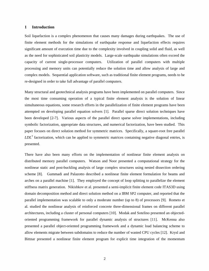
ParCYCLIC: Finite Element Modeling of Earthquake Liquefaction Response on Parallel Computers

Jun Peng1, Jinchi Lu2, Kincho H. Law3 and Ahmed Elgamal4

Abstract

This paper presents the computational procedures and solution strategy employed in ParCYCLIC, a

parallel nonlinear finite element program developed based on an existing serial code CYCLIC for the

analysis of cyclic seismically-induced liquefaction problems. In ParCYCLIC, finite elements are

employed within an incremental plasticity, coupled solid-fluid formulation. A constitutive model

developed for simulating liquefaction-induced deformations is a main component of this analysis

framework. The elements of the computational strategy, designed for distributed-memory message-

passing parallel computer systems, include: (a) an automatic domain decomposer to partition finite

element mesh; (b) nodal ordering strategies to minimize storage space for matrix coefficients; (c) an

efficient scheme for the allocation of sparse matrix coefficients among the processors; and (d) a parallel

sparse direct solver. Application of ParCYCLIC to simulate 3-D geotechnical experimental models is

demonstrated. Not only good agreement is achieved between the computed and recorded results, but also

the computational results show excellent parallel performance and scalability of ParCYCLIC on parallel

computers with large number of processors.

Keywords

Parallel computation, sparse matrix, finite element modeling, earthquake liquefaction, domain

decomposition

1 Research Associate, Department of Civil and Environmental Engineering, Stanford University, Stanford, CA 94305. Phone: (650) 725-1886, Fax: (650) 723-4806, E-mail: junpeng@stanford.edu. 2 Ph.D. Candidate, Department of Structural Engineering, University of California, San Diego, CA 92093. E-mail: jinlu@ucsd.edu. 3 Professor, Department of Civil and Environmental Engineering, Stanford University, Stanford, CA 94305. E-mail: law@stanford.edu. 4 Professor, Department of Structural Engineering, University of California, San Diego, CA 92093. E-mail: elgamal@ucsd.edu.

2

1 Introduction

Soil liquefaction is a complex phenomenon that causes many damages during earthquakes. The use of

finite element methods for the simulations of earthquake response and liquefaction effects requires

significant amount of execution time due to the complexity involved in coupling solid and fluid, as well

as the need for sophisticated soil plasticity models. Large-scale earthquake simulations often exceed the

capacity of current single-processor computers. Utilization of parallel computers with multiple

processing and memory units can potentially reduce the solution time and allow analysis of large and

complex models. Sequential application software, such as traditional finite element programs, needs to be

re-designed in order to take full advantage of parallel computers.

Many structural and geotechnical analysis programs have been implemented on parallel computers. Since

the most time consuming operation of a typical finite element analysis is the solution of linear

simultaneous equations, some research efforts in the parallelization of finite element programs have been

attempted on developing parallel equation solvers [1]. Parallel sparse direct solution techniques have

been developed [2-7]. Various aspects of the parallel direct sparse solver implementations, including

symbolic factorization, appropriate data structures, and numerical factorization, have been studied. This

paper focuses on direct solution method for symmetric matrices. Specifically, a square-root free parallel

LDLT factorization, which can be applied to symmetric matrices containing negative diagonal entries, is

presented.

There have also been many efforts on the implementation of nonlinear finite element analysis on

distributed memory parallel computers. Watson and Noor presented a computational strategy for the

nonlinear static and post-buckling analysis of large complex structures using nested dissection ordering

scheme [8]. Gummadi and Palazotto described a nonlinear finite element formulation for beams and

arches on a parallel machine [1]. They employed the concept of loop splitting to parallelize the element

stiffness matrix generation. Nikishkov et al. presented a semi-implicit finite element code ITAS3D using

domain decomposition method and direct solution method on a IBM SP2 computer, and reported that the

parallel implementation was scalable to only a moderate number (up to 8) of processors [9]. Rometo et

al. studied the nonlinear analysis of reinforced concrete three-dimensional frames on different parallel

architectures, including a cluster of personal computers [10]. Modak and Sotelino presented an objected-

oriented programming framework for parallel dynamic analysis of structures [11]. McKenna also

presented a parallel object-oriented programming framework and a dynamic load balancing scheme to

allow elements migrate between subdomains to reduce the number of wasted CPU cycles [12]. Krysl and

Bittnar presented a nonlinear finite element program for explicit time integration of the momentum

3

equations in structural dynamics [13]. Bao et al. modeled earthquake ground motion in large sedimentary

basins using a 3D linear finite element program with explicit integration method on parallel computers

and concluded that implicit method is not attractive on distributed memory computers [14].

This research presents the implementation of a parallel version of a geomechanics nonlinear finite

element program for the simulation of earthquake ground response and liquefaction effects. The

implementation is based on the serial program CYCLIC, which is a nonlinear finite element program

developed to analyze cyclic mobility and liquefaction problems [15, 16]. Extensive calibration of

CYCLIC has been conducted with results from experiments and full-scale response of earthquake

simulations involving ground liquefaction. CYCLIC program is re-designed and parallelized to form

ParCYCLIC. A parallel sparse direct solver has been incorporated to improve the simulation

performance. The objectives of developing ParCYCLIC are to extend the computational capabilities of

the finite element program to simulate large-scale systems, and to broaden the scope of its applications to

seismic ground-foundation interaction problems.

2 Theoretical Background of ParCYCLIC

The finite element formulation and the stress-strain model adopted in ParCYCLIC are the same as those

in CYCLIC. The theoretical development is based on the two phase (solid-fluid) fully-coupled finite

element formulation of Chan [17] and Zienkiewicz et al. [18]. The soil constitutive model incorporated is

developed specifically for liquefaction analysis [15, 19]. The current implementation is based on small-

deformation theory and does not account for nonlinear effects due to finite deformation or rotation. In the

following, the finite element formulation and the soil constitutive model adopted in CYCLIC and

ParCYCLIC are briefly described.

2.1 Finite Element Formulation

In CYCLIC and ParCYCLIC, the saturated soil system is modeled as a two-phase material based on the

Biot theory [20] for porous media. A numerical formulation of this theory, known as u-p formulation (in

which displacement of the soil skeleton u, and pore pressure p, are the primary unknowns [17, 18]), is

implemented [15, 16, 19]. This implementation is based on the following assumptions: small deformation

and rotation, constant density of the solid and fluid in both time and space, locally homogeneous porosity

which is constant with time, incompressibility of the soil grains, and equal accelerations for the solid and

fluid phases.

4

The u-p formulation is defined by Chan [17] as two equations: one is the equation of motion for the solid-

fluid mixture, and the other is the equation of mass conservation for the fluid phase that incorporates

equation of motion for the fluid phase and Darcy's law. These two governing equations can be expressed

in the following finite element matrix form [17]:

0fQpdΩ σBUM s

Ω

T =−+′+ ∫ (1a)

0fHppSUQ pT =−++ (1b)

where M is the total mass matrix, U the displacement vector, B the strain-displacement matrix, σ′ the

effective stress vector (determined by the soil constitutive model described below), Q the discrete

gradient operator coupling the solid and fluid phases, p the pore pressure vector, S the compressibility

matrix, and H the permeability matrix. The vectors sf and pf represent the effects of body forces and

prescribed boundary conditions for the solid-fluid mixture and the fluid phase, respectively.

In Equation 1a (equation of motion), the first term represents inertia force of the solid-fluid mixture,

followed by internal force due to soil skeleton deformation, and internal force induced by pore-fluid

pressure. In Equation 1b (equation of mass conservation), the first two terms represent the rate of volume

change for the soil skeleton and the fluid phase respectively, followed by the seepage rate of the pore

fluid. Equations 1a and 1b are integrated in the time space using a single-step predictor multi-corrector

scheme of the Newmark type [15, 17]. In the current implementation, the solution is obtained for each

time step using the modified Newton-Raphson approach [15].

2.2 Soil Constitutive Model

The second term in Equation 1a, which corresponds to the internal force due to soil deformation, is

defined by the soil stress-strain constitutive model. The finite element program incorporates a soil

constitutive model [15, 16, 21] based on the original multi-surface-plasticity theory for frictional

cohesionless soils [22]. This model was developed with emphasis on simulating the liquefaction-induced

shear strain accumulation mechanism in clean medium-dense sands [16, 21, 23, 24]. Special attention

was given to the deviatoric-volumetric strain coupling (dilatancy) under cyclic loading, which causes

increased shear stiffness and strength at large cyclic shear strain excursions (i.e., cyclic mobility).

The constitutive equation is written in incremental form as follows [22]:

)(: pεεEσ −=′ (2)

5

where σ ′ is the rate of effective Cauchy stress tensor, ε the rate of deformation tensor, pε the plastic

rate of deformation tensor, and E the isotropic fourth-order tensor of elastic coefficients. The rate of

plastic deformation tensor is defined by: pε = P L , where P is a symmetric second-order tensor

defining the direction of plastic deformation in stress space, L the plastic loading function, and the symbol

denotes the McCauley's brackets (i.e., L =max(L, 0)). The loading function L is defined as: L =

Q:σ ′ / H ′ where H ′ is the plastic modulus, and Q a unit symmetric second-order tensor defining yield-

surface normal at the stress point (i.e., Q= ff ∇∇ / ), with the yield function f written in the following

form:

0)())(())((2

3 20

200 =′+′−′+′−′+′−= ppMppppf αsαs : (3)

in the domain of 0≥′p [21]. The yield surfaces in principal stress space and deviatoric plane are shown

in Figure 1. In Equation 3, δσs p′−′= is the deviatoric stress tensor, p′ the mean effective stress, 0p′

a small positive constant (1.0 kPa in this paper) such that the yield surface size remains finite at 0=′p

for numerical convenience (Figure 1), α a second-order kinematic deviatoric tensor defining the surface

coordinates, and M dictates the surface size. In the context of multi-surface plasticity, a number of similar

surfaces with a common apex form the hardening zone (Figure 1). Each surface is associated with a

constant plastic modulus. Conventionally, the low-strain (elastic) module and the plastic module are

postulated to increase in proportion to the square root of p′ [22].

Figure 1. Conical Yield Surfaces for Granular Soils in Principal Stress Space and Deviatoric Plane

6

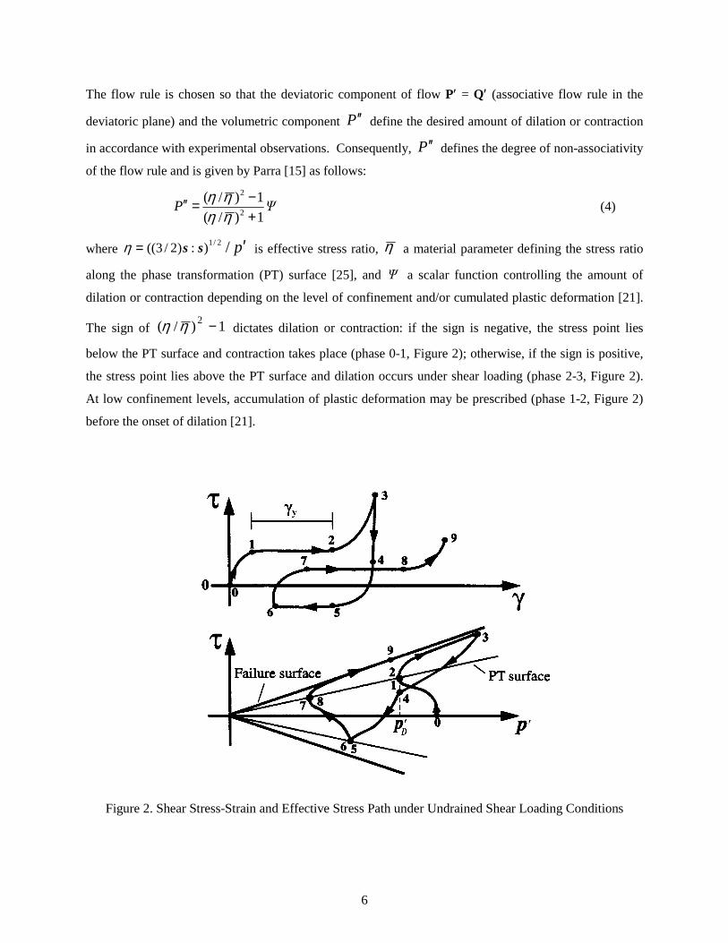
The flow rule is chosen so that the deviatoric component of flow P′ = Q′ (associative flow rule in the

deviatoric plane) and the volumetric component P ′′ define the desired amount of dilation or contraction

in accordance with experimental observations. Consequently, P ′′ defines the degree of non-associativity

of the flow rule and is given by Parra [15] as follows:

ΨP1)/(

1)/(2

2

+−=′′

ηηηη

(4)

where p′= /2/1):)2/3(( ssη is effective stress ratio, η a material parameter defining the stress ratio

along the phase transformation (PT) surface [25], and Ψ a scalar function controlling the amount of

dilation or contraction depending on the level of confinement and/or cumulated plastic deformation [21].

The sign of 1)/( 2 −ηη dictates dilation or contraction: if the sign is negative, the stress point lies

below the PT surface and contraction takes place (phase 0-1, Figure 2); otherwise, if the sign is positive,

the stress point lies above the PT surface and dilation occurs under shear loading (phase 2-3, Figure 2).

At low confinement levels, accumulation of plastic deformation may be prescribed (phase 1-2, Figure 2)

before the onset of dilation [21].

Figure 2. Shear Stress-Strain and Effective Stress Path under Undrained Shear Loading Conditions

7

A purely deviatoric kinematic hardening rule is chosen according to Prevost [22]:

µα bp =′ (5)

where µ is a deviatoric tensor defining the direction of translation and b is a scalar magnitude dictated

by the consistency condition. In order to enhance computational efficiency, the direction of translation

µ is defined by a new rule [15, 21], which maintains the concept of conjugate-points contact by Mroz

[26]. Thus, all yield surfaces may translate in stress space within the failure envelope

3 ParCYCLIC Software Organization

3.1 Parallel Program Strategies

Programming models required to take advantage of parallel computers are significantly different from the

traditional paradigm for a sequential program [27]. In a parallel computing environment, cares must be

taken to maintain all participating processors busy performing useful computations and to minimize

communication among the processors. To take advantage of parallel processing power, the algorithms

and data structures of CYCLIC are re-designed and implemented in ParCYCLIC.

One approach in developing application software for distributed memory parallel computers is to use the

single-program-multiple-data (SPMD) paradigm [28, 29]. The SPMD paradigm is related to the divide

and conquer strategy and is based on breaking a large problem into a number of smaller sub-problems,

which may be solved separately on individual processors. In this parallel programming paradigm, all

processors are assigned the same program code but run with different data sets comprising the problem.

A finite element domain is first decomposed using some well-known domain decomposition techniques.

Each processor of the parallel machine then solves a partitioned domain, and data communications among

sub-domains are performed through message passing. Domain decomposition is attractive in finite

element computations on parallel computers because it allows individual sub-domain operations to be

performed concurrently on separate processors. The SPMD model has been applied successfully in the

development of many parallel finite element programs from legacy serial codes [28, 30]. The

development of ParCYCLIC follows the SPMD model to parallelize the legacy serial code CYCLIC.

3.2 Computational Procedures

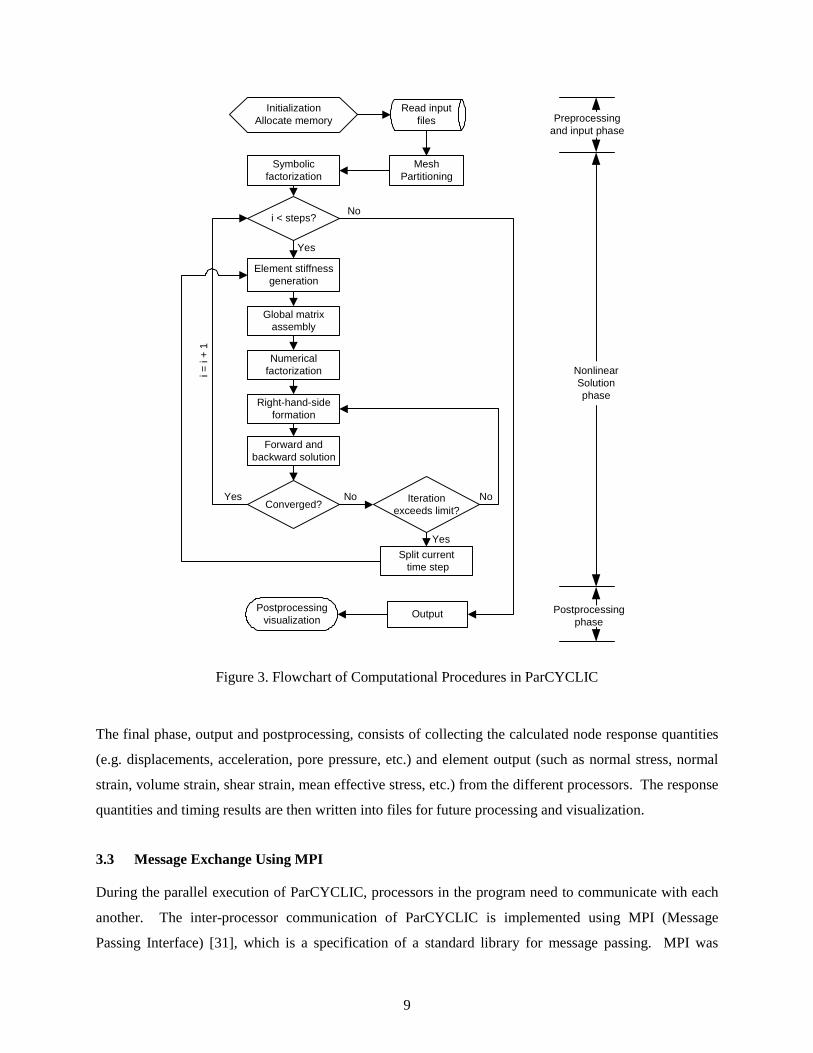
The computational procedure of ParCYCLIC is illustrated in Figure 3. The procedure can be divided into

three phases, namely: preprocessing and input phase, nonlinear solution phase, and output and

postprocessing phase. The first phase consists of initializing certain variables, allocating memories, and

reading the input file. There is no inter-process communication involved in this phase – all the processors

8

run the same piece of code and read identical copies of the same input file. Since a mesh partitioning

routine is incorporated in ParCYCLIC, the input file does not need to contain any information for

processor assignment of nodes and elements. The input file for ParCYCLIC has essentially the same

format as that of CYCLIC.

After the preprocessing and input phase, the nonlinear solution phase starts with using a domain

decomposer to partition the finite element mesh. Symbolic factorization is then performed to determine

the nonzero pattern of the matrix factor. After the symbolic factorization, the storage spaces for the

sparse matrix factor required by each processor are allocated. Since all the processors need to know the

nonzero pattern of the global stiffness matrix and symbolic factorization generally only takes a small

portion of the total runtime, each processor carries out the domain decomposition and symbolic

factorization based on the global data.

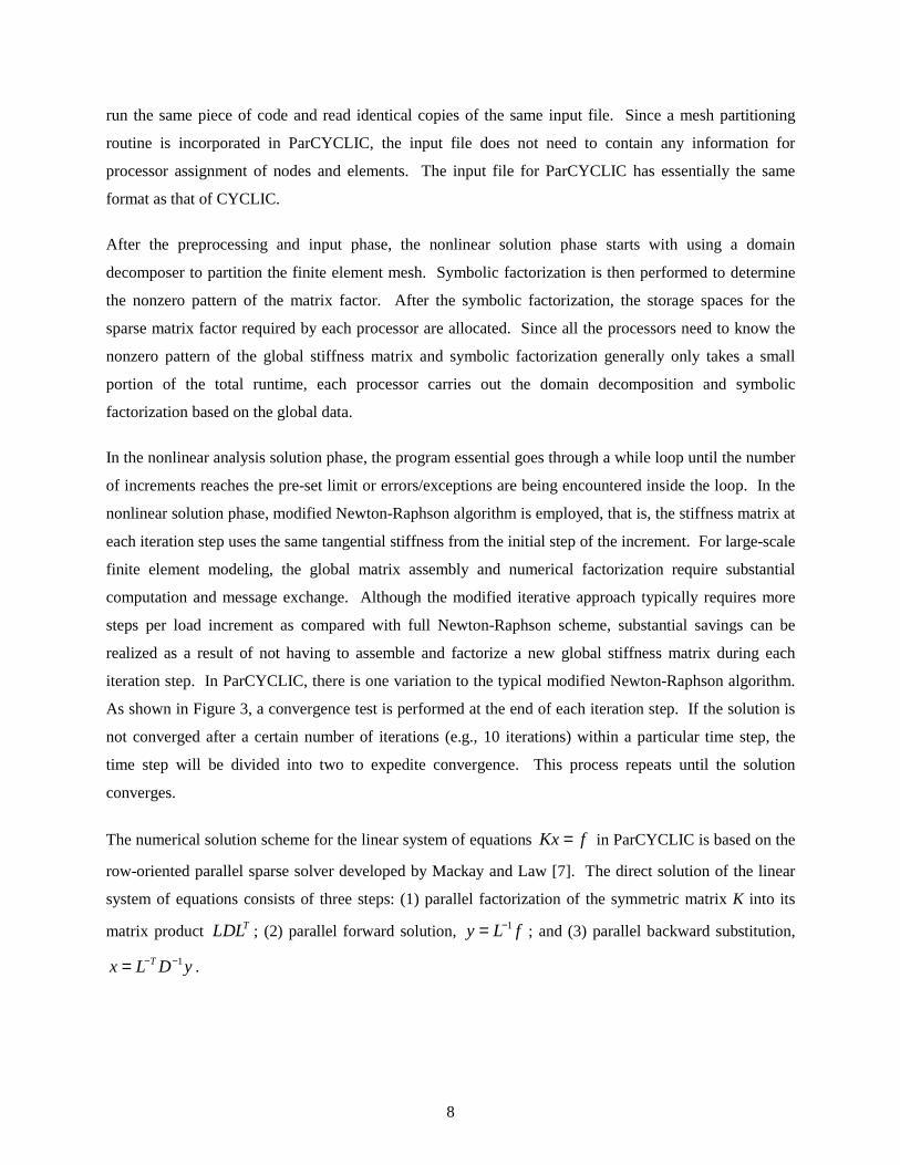
In the nonlinear analysis solution phase, the program essential goes through a while loop until the number

of increments reaches the pre-set limit or errors/exceptions are being encountered inside the loop. In the

nonlinear solution phase, modified Newton-Raphson algorithm is employed, that is, the stiffness matrix at

each iteration step uses the same tangential stiffness from the initial step of the increment. For large-scale

finite element modeling, the global matrix assembly and numerical factorization require substantial

computation and message exchange. Although the modified iterative approach typically requires more

steps per load increment as compared with full Newton-Raphson scheme, substantial savings can be

realized as a result of not having to assemble and factorize a new global stiffness matrix during each

iteration step. In ParCYCLIC, there is one variation to the typical modified Newton-Raphson algorithm.

As shown in Figure 3, a convergence test is performed at the end of each iteration step. If the solution is

not converged after a certain number of iterations (e.g., 10 iterations) within a particular time step, the

time step will be divided into two to expedite convergence. This process repeats until the solution

converges.

The numerical solution scheme for the linear system of equations Kx f= in ParCYCLIC is based on the

row-oriented parallel sparse solver developed by Mackay and Law [7]. The direct solution of the linear

system of equations consists of three steps: (1) parallel factorization of the symmetric matrix K into its

matrix product TLDL ; (2) parallel forward solution, 1y L f−= ; and (3) parallel backward substitution,

1Tx L D y− −= .

9

Symbolicfactorization

Postprocessingvisualization

Global matrixassembly

Numericalfactorization

Right-hand-sideformation

Forward andbackward solution

Converged?

Read inputfiles

InitializationAllocate memory

i < steps?No

Element stiffnessgeneration

Yes

Yes

i = i

+ 1

Iterationexceeds limit?

No

Split current time step

Yes

No

Preprocessingand input phase

NonlinearSolutionphase

Postprocessingphase

Output

MeshPartitioning

Figure 3. Flowchart of Computational Procedures in ParCYCLIC

The final phase, output and postprocessing, consists of collecting the calculated node response quantities

(e.g. displacements, acceleration, pore pressure, etc.) and element output (such as normal stress, normal

strain, volume strain, shear strain, mean effective stress, etc.) from the different processors. The response

quantities and timing results are then written into files for future processing and visualization.

3.3 Message Exchange Using MPI

During the parallel execution of ParCYCLIC, processors in the program need to communicate with each

another. The inter-processor communication of ParCYCLIC is implemented using MPI (Message

Passing Interface) [31], which is a specification of a standard library for message passing. MPI was

10

defined by the MPI Forum, a broadly based group of parallel computer vendors, library developers, and

applications specialists. One advantage of MPI is its portability, which makes it suitable to develop

programs to run on a wide range of parallel computers and workstation clusters. Another advantage of

MPI is its performance, because each MPI implementation is optimized for the hardware it runs on.

Generally, MPI code can be developed for an arbitrary number of processors. It is up to the users to

decide, at run-time, how many processors should be invoked for the execution.

The MPI library consists of a large set of message passing primitives (functions) to support efficient

parallel processes running on a large number of processors interconnected over a network. The

implementation of ParCYCLIC employs only a small set of MPI message passing functions. There are

two types of communications in ParCYCLIC: point-to-point communication and collective messages.

The point-to-point communication in MPI involves the transmittal of data between two processors. The

collective communications, on the other hand, transmit data among all processors in a group.

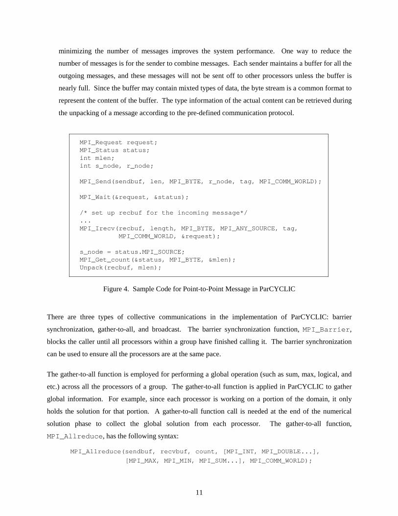
For the implementation of ParCYCLIC, point-to-point messages are used extensively during the global

matrix assembly and matrix factorization phases. Figure 4 shows some sample codes for the point-to-

point messages in ParCYCLIC, which have the following features:

• For most of the point-to-point communications, the blocking send (MPI_Send) is used to send out

data, and the non-blocking receive (MPI_Irecv) is used to receive data. The purpose of this choice

is to keep all the processors busy performing useful computation and at the same time to ensure all

the messages are delivered. A blocking send temporarily stores the message data in a buffer. The

function does not return until the message has been safely delivered. A non-blocking receive tests the

buffer for any incoming messages, and can concurrently perform computation not relying on the

incoming messages.

• The MPI_Send sends a message to the specific recipient by passing the receiver’s node

identification (denoted as r_node in Figure 4) as one of the parameters. The MPI_Irecv, on the

other hand, receives a message from any source by denoting the sender as a wild card value of

MPI_ANY_SOURCE. The sender knows whom the recipient is when sending a particular message,

while the receiver listens to messages from all processors. After a message is received, the

MPI_SOURCE field of the MPI_Status is retrieved to find the node identification of the sender.

The actual size of the received message is detected by calling the function MPI_Get_count.

• Instead of sending messages with data type information (such as double, integer, byte, etc.), all data

are sent as a byte stream, which is denoted as MPI_BYTE. Since messages have overhead cost,

11

minimizing the number of messages improves the system performance. One way to reduce the

number of messages is for the sender to combine messages. Each sender maintains a buffer for all the

outgoing messages, and these messages will not be sent off to other processors unless the buffer is

nearly full. Since the buffer may contain mixted types of data, the byte stream is a common format to

represent the content of the buffer. The type information of the actual content can be retrieved during

the unpacking of a message according to the pre-defined communication protocol.

MPI_Request request; MPI_Status status; int mlen; int s_node, r_node; MPI_Send(sendbuf, len, MPI_BYTE, r_node, tag, MPI_COMM_WORLD); MPI_Wait(&request, &status); /* set up recbuf for the incoming message*/ ... MPI_Irecv(recbuf, length, MPI_BYTE, MPI_ANY_SOURCE, tag, MPI_COMM_WORLD, &request);

s_node = status.MPI_SOURCE; MPI_Get_count(&status, MPI_BYTE, &mlen); Unpack(recbuf, mlen);

Figure 4. Sample Code for Point-to-Point Message in ParCYCLIC

There are three types of collective communications in the implementation of ParCYCLIC: barrier

synchronization, gather-to-all, and broadcast. The barrier synchronization function, MPI_Barrier,

blocks the caller until all processors within a group have finished calling it. The barrier synchronization

can be used to ensure all the processors are at the same pace.

The gather-to-all function is employed for performing a global operation (such as sum, max, logical, and

etc.) across all the processors of a group. The gather-to-all function is applied in ParCYCLIC to gather

global information. For example, since each processor is working on a portion of the domain, it only

holds the solution for that portion. A gather-to-all function call is needed at the end of the numerical

solution phase to collect the global solution from each processor. The gather-to-all function,

MPI_Allreduce, has the following syntax:

MPI_Allreduce(sendbuf, recvbuf, count, [MPI_INT, MPI_DOUBLE...],

[MPI_MAX, MPI_MIN, MPI_SUM...], MPI_COMM_WORLD);

12

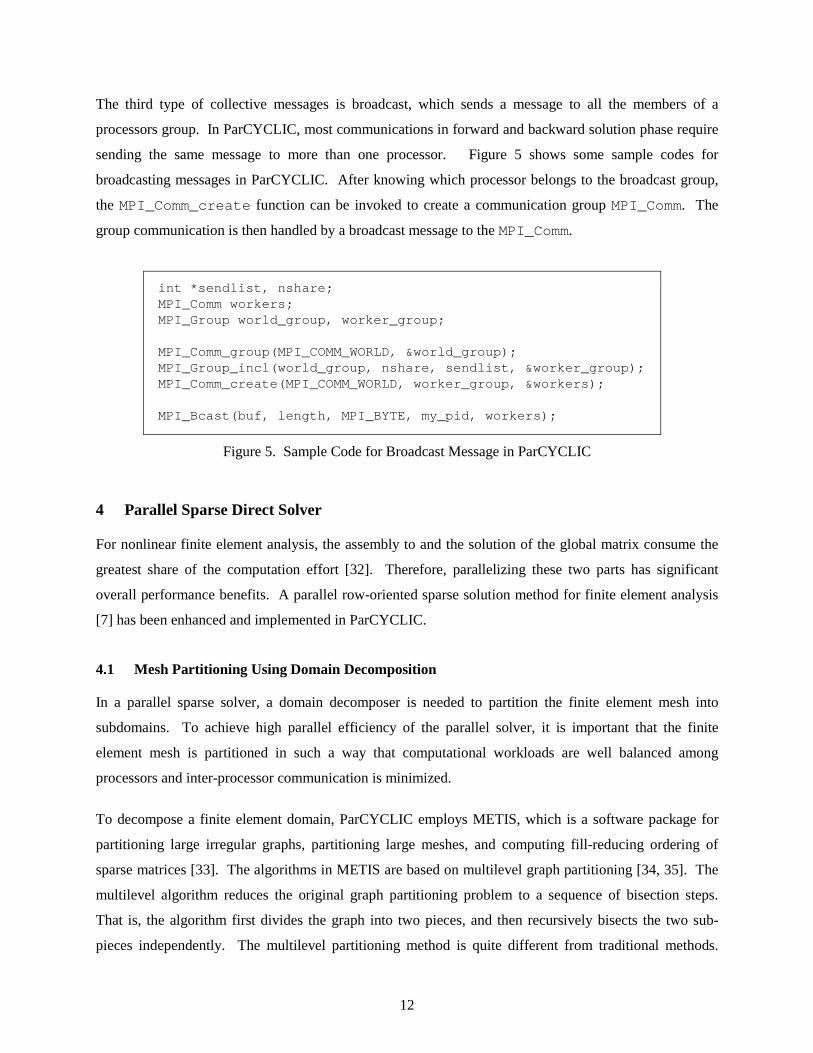
The third type of collective messages is broadcast, which sends a message to all the members of a

processors group. In ParCYCLIC, most communications in forward and backward solution phase require

sending the same message to more than one processor. Figure 5 shows some sample codes for

broadcasting messages in ParCYCLIC. After knowing which processor belongs to the broadcast group,

the MPI_Comm_create function can be invoked to create a communication group MPI_Comm. The

group communication is then handled by a broadcast message to the MPI_Comm.

int *sendlist, nshare; MPI_Comm workers; MPI_Group world_group, worker_group; MPI_Comm_group(MPI_COMM_WORLD, &world_group); MPI_Group_incl(world_group, nshare, sendlist, &worker_group); MPI_Comm_create(MPI_COMM_WORLD, worker_group, &workers); MPI_Bcast(buf, length, MPI_BYTE, my_pid, workers);

Figure 5. Sample Code for Broadcast Message in ParCYCLIC

4 Parallel Sparse Direct Solver

For nonlinear finite element analysis, the assembly to and the solution of the global matrix consume the

greatest share of the computation effort [32]. Therefore, parallelizing these two parts has significant

overall performance benefits. A parallel row-oriented sparse solution method for finite element analysis

[7] has been enhanced and implemented in ParCYCLIC.

4.1 Mesh Partitioning Using Domain Decomposition

In a parallel sparse solver, a domain decomposer is needed to partition the finite element mesh into

subdomains. To achieve high parallel efficiency of the parallel solver, it is important that the finite

element mesh is partitioned in such a way that computational workloads are well balanced among

processors and inter-processor communication is minimized.

To decompose a finite element domain, ParCYCLIC employs METIS, which is a software package for

partitioning large irregular graphs, partitioning large meshes, and computing fill-reducing ordering of

sparse matrices [33]. The algorithms in METIS are based on multilevel graph partitioning [34, 35]. The

multilevel algorithm reduces the original graph partitioning problem to a sequence of bisection steps.

That is, the algorithm first divides the graph into two pieces, and then recursively bisects the two sub-

pieces independently. The multilevel partitioning method is quite different from traditional methods.

13

Traditional graph partitioning algorithms compute a partition of a graph by operating directly on the

original graph. Multilevel partitioning algorithm, on the other hand, takes a different approach. First, the

algorithm reduces the size of the graph by collapsing vertices and edges to produce a smaller graph. The

graph partitioning is then performed on the collapsed graph. Finally, the partition is propagated back

through the sequence to un-collapse the vertices and edges, with an occasional local refinement [33].

METIS provides both stand-alone programs (executable files) and library interfaces (functions). The

library interfaces are incorporated in ParCYCLIC to perform the domain decomposition. In particular,

multilevel k-way partitioning routine is used in ParCYCLIC to partition a graph into k parts. The number

of processors (power of 2 is suggested) used in the execution of ParCYCLIC determines the number of

levels to partition. The objective of the partitioning is to minimize the total communication volume.

Once the cuts are found by METIS routines, i.e., the finite element mesh has been partitioned into

subdomains, the internal nodes of each subdomain still need to be ordered to reduce the fill-ins of the

matrix factors. There are many ordering routines implemented in ParCYCLIC to perform this task,

including Reverse Cuthill-McKee [36], Minimum Degree [37], General Nested Dissection [38], and

Multilevel Nested Dissection [34]. Users are allowed to choose different types of ordering routines for a

specific problem. Otherwise, the default ordering routine is the Multilevel Nested Dissection ordering,

because it is stable and normally generates an ordering with the least fill-ins of the matrix factors. After

the matrix ordering is complete, symbolic factorization and parallel matrix assignment are performed.

4.2 Assignment of Sparse Stiffness Matrix

The notion of the elimination tree plays a significant role in sparse matrix study [39]. It is well known

that the nonzero entries in the numerical factor L can be determined by the original nonzero entries of the

stiffness matrix K [40, 41] and a list vector, which is defined as

0|min)( ≠= ijLijPARENT (6)

The array PARENT represents the row subscript of the first nonzero entry in each column of the lower

triangular matrix factor L. The definition of the list array PARENT results in a monotonically ordered

elimination tree of which each node has its numbering higher than its descendants. By topologically post-

ordering the elimination tree, the nodes in any subtree can be numbered consecutively. The resulting

sparse matrix factor is partitioned into block submatrices where the columns/row of each block

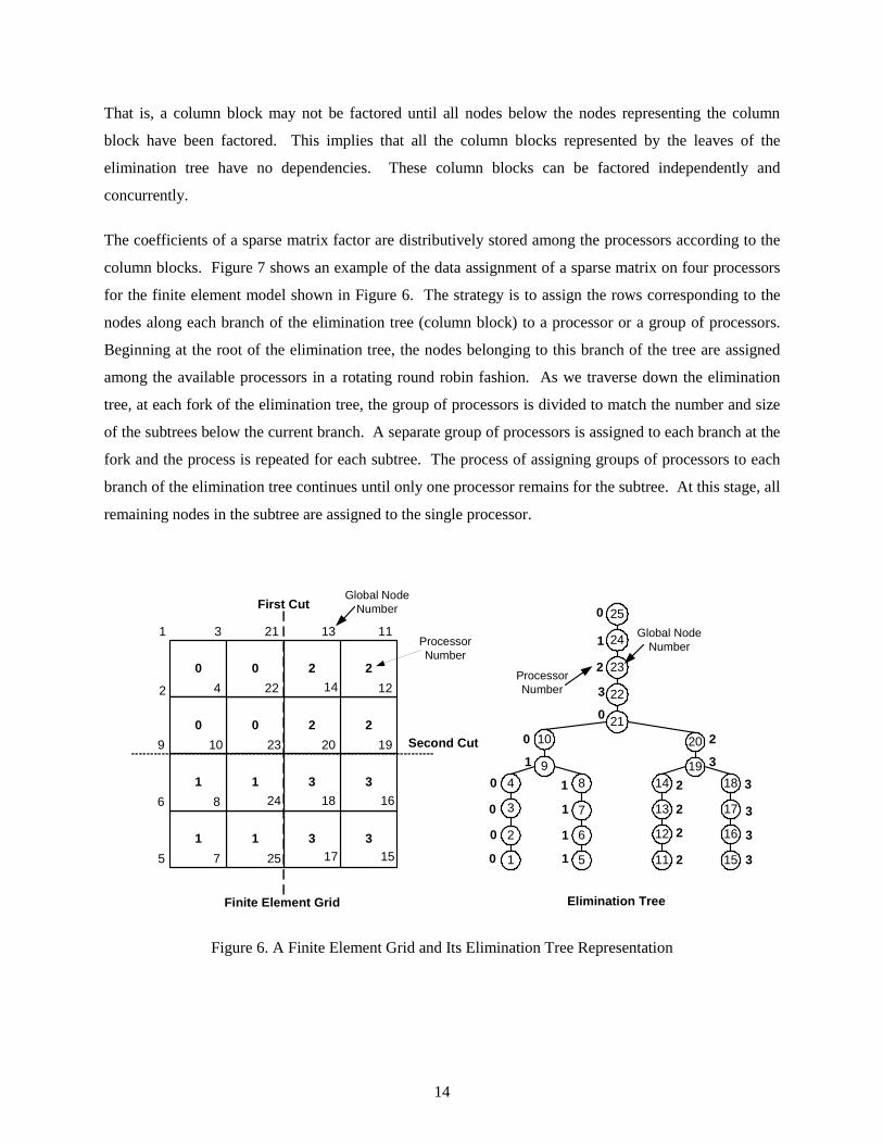
corresponds to the node set of a branch in the elimination tree. Figure 6 shows a simple square finite

element grid and its post-ordered elimination tree representation. One important feature of the

elimination tree is that it describes the dependencies among the variables during the factorization process.

14

That is, a column block may not be factored until all nodes below the nodes representing the column

block have been factored. This implies that all the column blocks represented by the leaves of the

elimination tree have no dependencies. These column blocks can be factored independently and

concurrently.

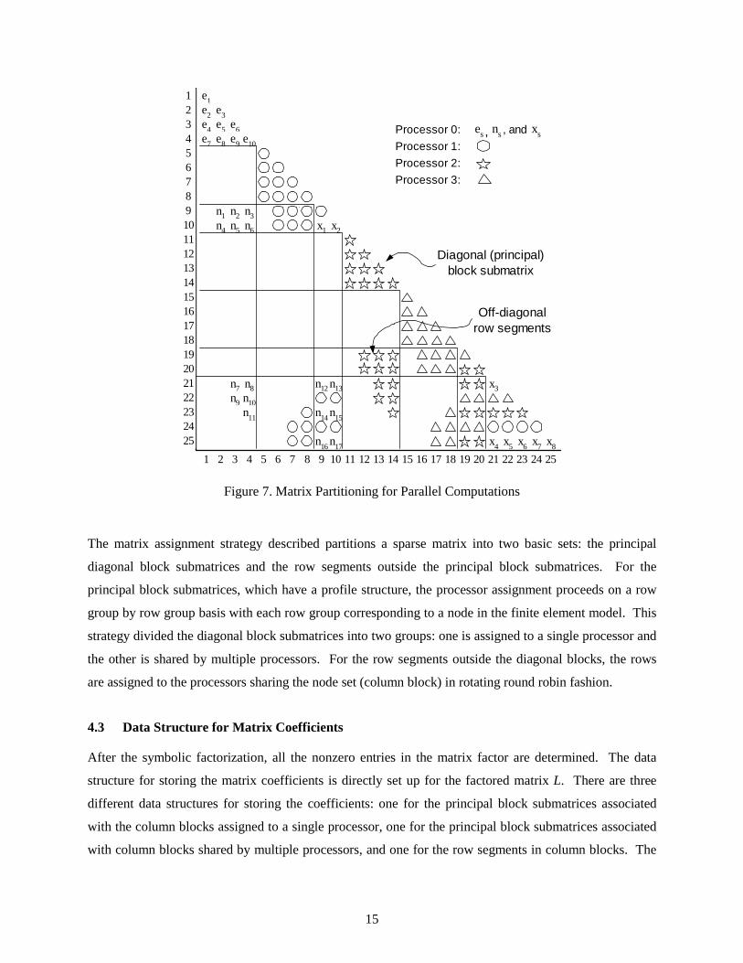
The coefficients of a sparse matrix factor are distributively stored among the processors according to the

column blocks. Figure 7 shows an example of the data assignment of a sparse matrix on four processors

for the finite element model shown in Figure 6. The strategy is to assign the rows corresponding to the

nodes along each branch of the elimination tree (column block) to a processor or a group of processors.

Beginning at the root of the elimination tree, the nodes belonging to this branch of the tree are assigned

among the available processors in a rotating round robin fashion. As we traverse down the elimination

tree, at each fork of the elimination tree, the group of processors is divided to match the number and size

of the subtrees below the current branch. A separate group of processors is assigned to each branch at the

fork and the process is repeated for each subtree. The process of assigning groups of processors to each

branch of the elimination tree continues until only one processor remains for the subtree. At this stage, all

remaining nodes in the subtree are assigned to the single processor.

0

331

331

1

1

2200

220

1

9

2

First Cut

Second Cut20

14

13

25

24

23

22

21

7

8

10

4

3

5

6

17

18

15

16

19

11

12

25

9181484

201021

22

23

24

2

171373

19

15

16

11

12

1 5

6

Global NodeNumber

ProcessorNumber

Finite Element Grid Elimination Tree

Global NodeNumber

1 3

3

3

3

32

2

2

2

0

1

1

1

1

0

0

0

0

2

0

1

2

3

0

ProcessorNumber

Figure 6. A Finite Element Grid and Its Elimination Tree Representation

15

e1

e4

e2

e7

e5

n4

n1

e3

e8

n13

x2

n17

n15

x4 x5

n10

n8

n6

n3

e10

n11

e6

n9

n7

n5

n2

e9

n12

x1

n16

n14

x3

x6 x7 x8

1

3

2221201918171615141312111098765

2

4

252423

1 3 22212019181716151413121110987652 4 252423

Processor 0:

Processor 1:

Processor 2:

Processor 3:

es ns xs, , and

Diagonal (principal)block submatrix

Off-diagonalrow segments

Figure 7. Matrix Partitioning for Parallel Computations

The matrix assignment strategy described partitions a sparse matrix into two basic sets: the principal

diagonal block submatrices and the row segments outside the principal block submatrices. For the

principal block submatrices, which have a profile structure, the processor assignment proceeds on a row

group by row group basis with each row group corresponding to a node in the finite element model. This

strategy divided the diagonal block submatrices into two groups: one is assigned to a single processor and

the other is shared by multiple processors. For the row segments outside the diagonal blocks, the rows

are assigned to the processors sharing the node set (column block) in rotating round robin fashion.

4.3 Data Structure for Matrix Coefficients

After the symbolic factorization, all the nonzero entries in the matrix factor are determined. The data

structure for storing the matrix coefficients is directly set up for the factored matrix L. There are three

different data structures for storing the coefficients: one for the principal block submatrices associated

with the column blocks assigned to a single processor, one for the principal block submatrices associated

with column blocks shared by multiple processors, and one for the row segments in column blocks. The

16

following describes the details of these three different data structures. For demonstration purpose, the

data structure in Processor 0 for the square grid problem shown in Figure 7 is presented.

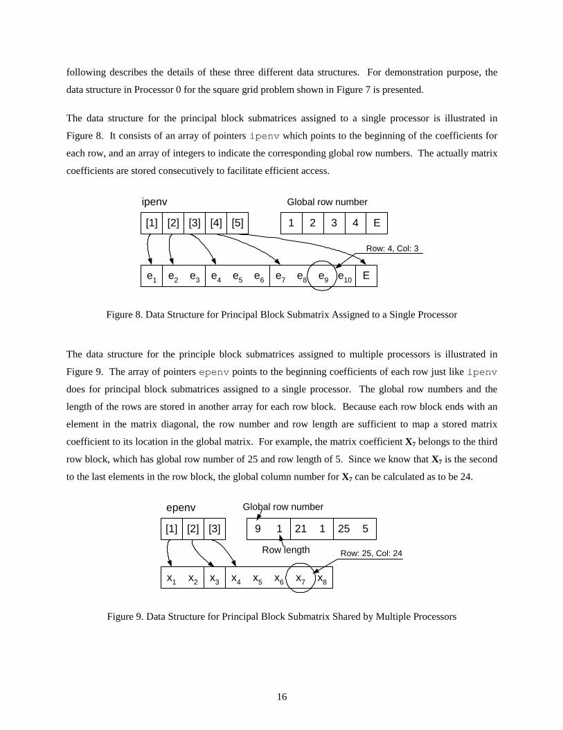
The data structure for the principal block submatrices assigned to a single processor is illustrated in

Figure 8. It consists of an array of pointers ipenv which points to the beginning of the coefficients for

each row, and an array of integers to indicate the corresponding global row numbers. The actually matrix

coefficients are stored consecutively to facilitate efficient access.

e1

[3][2][1]

Ee10e9e8e7e6e5e4e3e2

[4] [5]

ipenv

321 4 E

Global row number

Row: 4, Col: 3

Figure 8. Data Structure for Principal Block Submatrix Assigned to a Single Processor

The data structure for the principle block submatrices assigned to multiple processors is illustrated in

Figure 9. The array of pointers epenv points to the beginning coefficients of each row just like ipenv

does for principal block submatrices assigned to a single processor. The global row numbers and the

length of the rows are stored in another array for each row block. Because each row block ends with an

element in the matrix diagonal, the row number and row length are sufficient to map a stored matrix

coefficient to its location in the global matrix. For example, the matrix coefficient X7 belongs to the third

row block, which has global row number of 25 and row length of 5. Since we know that X7 is the second

to the last elements in the row block, the global column number for X7 can be calculated as to be 24.

x1

[3][2][1]

x8x7x6x5x4x3

epenv

9 1 525121

Global row number

Row length Row: 25, Col: 24

x2

Figure 9. Data Structure for Principal Block Submatrix Shared by Multiple Processors

17

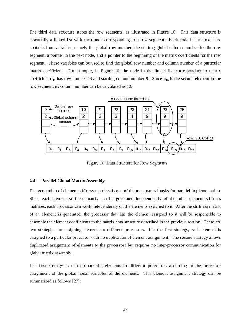
The third data structure stores the row segments, as illustrated in Figure 10. This data structure is

essentially a linked list with each node corresponding to a row segment. Each node in the linked list

contains four variables, namely the global row number, the starting global column number for the row

segment, a pointer to the next node, and a pointer to the beginning of the matrix coefficients for the row

segment. These variables can be used to find the global row number and column number of a particular

matrix coefficient. For example, in Figure 10, the node in the linked list corresponding to matrix

coefficient n15 has row number 23 and starting column number 9. Since n15 is the second element in the

row segment, its column number can be calculated as 10.

21

3

n1 n11n10n9n8n7n6n5n4n3n2 n17n16n15n14n13n12

9

2

10

2

22

3

23

4

21

9

23

9

25

9

Global rownumber

Global columnnumber

Row: 23, Col: 10

A node in the linked list

Figure 10. Data Structure for Row Segments

4.4 Parallel Global Matrix Assembly

The generation of element stiffness matrices is one of the most natural tasks for parallel implementation.

Since each element stiffness matrix can be generated independently of the other element stiffness

matrices, each processor can work independently on the elements assigned to it. After the stiffness matrix

of an element is generated, the processor that has the element assigned to it will be responsible to

assemble the element coefficients to the matrix data structure described in the previous section. There are

two strategies for assigning elements to different processors. For the first strategy, each element is

assigned to a particular processor with no duplication of element assignment. The second strategy allows

duplicated assignment of elements to the processors but requires no inter-processor communication for

global matrix assembly.

The first strategy is to distribute the elements to different processors according to the processor

assignment of the global nodal variables of the elements. This element assignment strategy can be

summarized as follows [27]:

18

1. If all the nodal variables of an element belong to a single processor, the element is assigned to that

processor.

2. If one of the nodal variables of an element belongs to a column block assigned to a single processor,

then the element is assigned to that processor.

3. If all nodal variables of an element are shared among multiple processors, the element is assigned to

the processor which is assigned the lowest global number variable of the element stiffness matrix.

For the parallel global matrix assembly, coefficients of the element stiffness matrices that belong to the

processor where the element stiffness matrix is formed are assembled into the global stiffness matrix

directly. If the coefficients of the element stiffness matrix belong to the segment of the global stiffness

matrix located in another processor, they are sent to that processor for assembly.

The first element assignment strategy ensures no duplication of element stiffness generation, but

substantial amount of messages are needed to exchange the stiffness matrix coefficients among the

processors. To eliminate the messages for global matrix assembly, a second element assignment strategy

is introduced in ParCYCLIC. All the elements along a cut are assigned to a group of processors that

share the cut. In this strategy, the same element may be assigned to more than one processor, and

consequently the element stiffness generation will be duplicated. However, the duplication of work can

be offset by not having to exchange messages. During the global matrix assembly phase, coefficients of

the element stiffness matrices that belong to the processor where the element stiffness matrix is formed

are assembled into the global stiffness matrix directly. If the coefficients of the element stiffness matrix

belong to another processor, they are simply discarded.

Both strategies for element assignment have been implemented in ParCYCLIC. For illustration purpose,

Figure 11 shows the results of applying both strategies to assign elements to four processors for the

square grid model. Depending on the characteristics of the finite element model, users can choose which

strategy to be used. For large finite element models where the interface (cuts) is relatively small (in other

words, most of the elements have all their nodes assigned to a single processor), strategy two is

recommended. From the performance point of view, the performance overhead is small because the

number of duplicated elements is only a small portion of the total number of elements. From the

execution point of view, strategy two incurs no communication and thus easier to guarantee the

completion of matrix assembly.

19

0

331

331

1

1

2200

220

1

9

2

20

14

13

25

24

23

22

21

7

8

10

4

3

5

6

17

18

15

16

19

11

12

Global NodeNumber

ProcessorNumber

0

30,1,2,30,1,2,3

2,30,1,2,30,1,2,3

1

0,1

2,30,1,2,30,1,2,30,1

20,1,2,30,1,2,3

1

9

2

20

14

13

25

24

23

22

21

7

8

10

4

3

5

6

17

18

15

16

19

11

12

Global NodeNumber

ProcessorNumber

(a). Assignment of elements without duplication (b). Assignment of elements with duplication

Figure 11. Two Methods of Assigning Elements to Four Processors

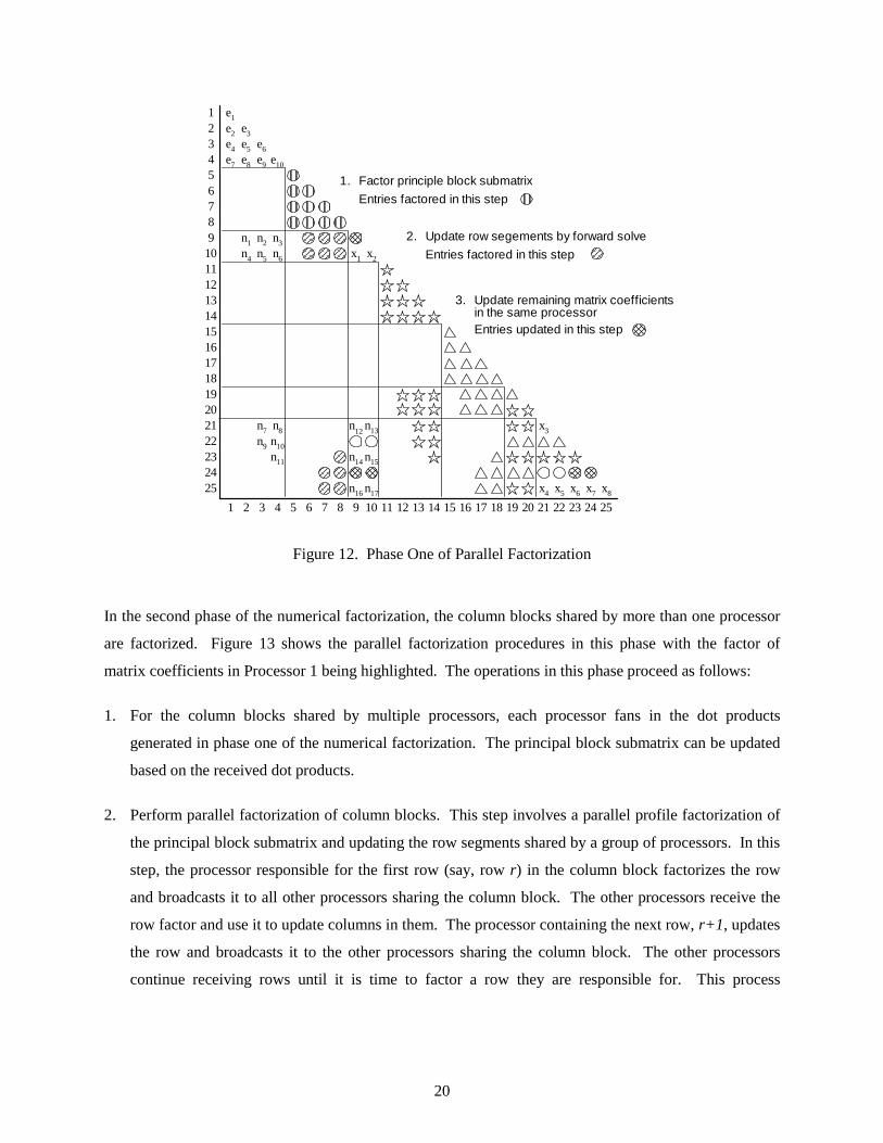
4.5 Parallel Numerical Factorization

Once the processor assignment and the assembly of the global stiffness matrix are completed, numerical

calculation can proceed. In ParCYCLIC, the TLDL factorization is performed. The parallel numerical

factorization procedure is divided into two distinct phases. During the first phase, the column blocks

assigned entirely to a single processor are factorized. The strategy is to carry out as much computation as

possible in the local processor. Figure 12 shows the parallel factorization procedures in this phase with

the factor of matrix coefficients in Processor 1 being highlighted. The operations in this phase are as

follows:

1. For each column block assigned to a processor, perform a profile factorization on principal block

submatrix.

2. Update the off-diagonal row segments below the principal submatrix by a series of forward solutions.

3. After the column blocks are factorized, form dot products among row segments. These dot products

are then fanned-out to update the remaining matrix coefficients in the same processor or saved in the

buffer to be sent out to other processor during the parallel factorization phase.

20

e1

e4

e2

e7

e5

n4

n1

e3

e8

n13

x2

n17

n15

x4 x5

n10

n8

n6

n3

e10

n11

e6

n9

n7

n5

n2

e9

n12

x1

n16

n14

x3

x6 x7 x8

1

3

2221201918171615141312111098765

2

4

252423

1 3 22212019181716151413121110987652 4 252423

2. Update row segements by forward solve

Entries factored in this step

3. Update remaining matrix coefficientsin the same processorEntries updated in this step

1. Factor principle block submatrix

Entries factored in this step

Figure 12. Phase One of Parallel Factorization

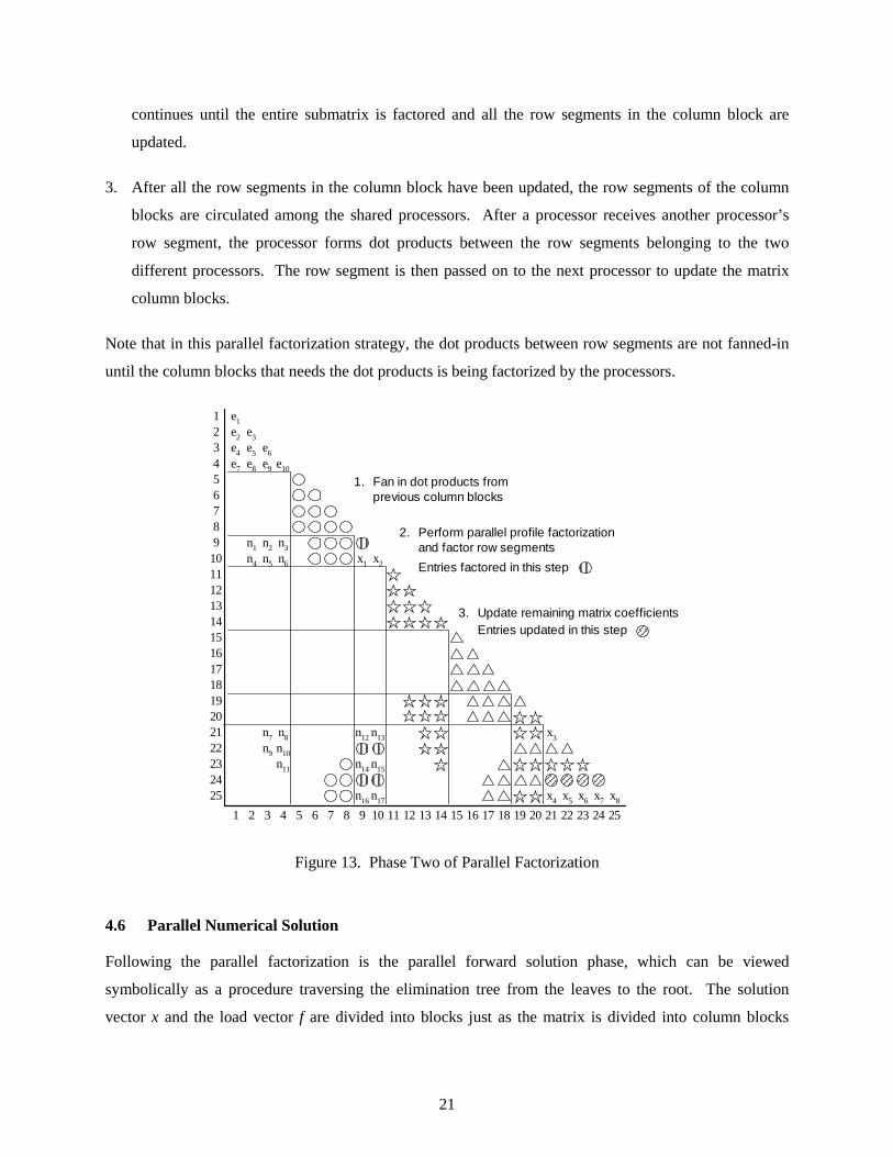
In the second phase of the numerical factorization, the column blocks shared by more than one processor

are factorized. Figure 13 shows the parallel factorization procedures in this phase with the factor of

matrix coefficients in Processor 1 being highlighted. The operations in this phase proceed as follows:

1. For the column blocks shared by multiple processors, each processor fans in the dot products

generated in phase one of the numerical factorization. The principal block submatrix can be updated

based on the received dot products.

2. Perform parallel factorization of column blocks. This step involves a parallel profile factorization of

the principal block submatrix and updating the row segments shared by a group of processors. In this

step, the processor responsible for the first row (say, row r) in the column block factorizes the row

and broadcasts it to all other processors sharing the column block. The other processors receive the

row factor and use it to update columns in them. The processor containing the next row, r+1, updates

the row and broadcasts it to the other processors sharing the column block. The other processors

continue receiving rows until it is time to factor a row they are responsible for. This process

21

continues until the entire submatrix is factored and all the row segments in the column block are

updated.

3. After all the row segments in the column block have been updated, the row segments of the column

blocks are circulated among the shared processors. After a processor receives another processor’s

row segment, the processor forms dot products between the row segments belonging to the two

different processors. The row segment is then passed on to the next processor to update the matrix

column blocks.

Note that in this parallel factorization strategy, the dot products between row segments are not fanned-in

until the column blocks that needs the dot products is being factorized by the processors.

e1

e4

e2

e7

e5

n4

n1

e3

e8

n13

x2

n17

n15

x4 x5

n10

n8

n6

n3

e10

n11

e6

n9

n7

n5

n2

e9

n12

x1

n16

n14

x3

x6 x7 x8

1

3

2221201918171615141312111098765

2

4

252423

1 3 22212019181716151413121110987652 4 252423

1. Fan in dot products fromprevious column blocks

2. Perform parallel profile factorizationand factor row segments

Entries factored in this step

3. Update remaining matrix coefficientsEntries updated in this step

Figure 13. Phase Two of Parallel Factorization

4.6 Parallel Numerical Solution

Following the parallel factorization is the parallel forward solution phase, which can be viewed

symbolically as a procedure traversing the elimination tree from the leaves to the root. The solution

vector x and the load vector f are divided into blocks just as the matrix is divided into column blocks

22

determined by the elimination tree. The forward solution phase is also divided into two phases: a

sequential phase and a parallel phase.

In the first phase, each processor calculates the blocks of f corresponding to the matrix blocks which

reside entirely within a single processor. For each column block assigned to a processor, each processor

performs a profile forward solve with the principal submatrix in the column block. Each processor also

updates the shared portions of the solution vector based on the row segments that lie below the profile

submatrices. The solution coefficients not assigned to this processor are stored in buffer to be sent to

other processors.

Phase two of the parallel forward solution begins as the processors working together on the variables in

the shared column blocks. There are three steps involved in this phase as outlined below:

1. The first step is to send and receive solution coefficients generated in phase one of the forward

solution. These coefficients are used to update the partially solved block of solution vector f.

2. The second step performs parallel forward solution based on principal submatrix. As each value of f

is calculated, for example f [i], it is broadcast to the other processors sharing the block. After

receiving the value of f [i], the processor responsible for f [i+1] can complete the solution and

broadcast the value to other processors sharing the column block. This process is repeated until the

solution to the entire block is completed.

3. The third step is to use the values in this block to update other blocks using the rows segments in this

column block.

Following the forward solution phase is the backward substitution procedure, which is essentially a

reverse of the forward solution. The first phase of backward substitution deals with the portion of the

solution vector shared by multiple processors and is essentially a reverse of the second phase of the

forward solution. In the second phase, each processor calculates the portion of the solution vector

corresponding to the column blocks residing within a single processor; the processors perform the

calculations independently without any processor communications and may complete the solution at

different times. Once all the processors finish the backward substitution, a global gathering function is

invoked to obtain the global solution from each processor. This step is essential because each processor

only has part of the global solution vector that it is responsible for.

23

5 Performance of ParCYCLIC

To demonstrate the simulation capability and parallel performance of ParCYCLIC, we have performed

earthquake simulations for three-dimensional geotechnical models using ParCYCLIC. The simulations

are performed on the Blue Horizon machine at San Diego Supercomputer Center. Blue Horizon is an

IBM Scalable POWERparallel (SP) machine which has 144 compute nodes, each with 8 POWER3 RISC-

based processors and with 4 GBytes of memory. Each processor on the node has equal shared access to

the memory. The following presents the simulations of two 3D geotechnical finite element models.

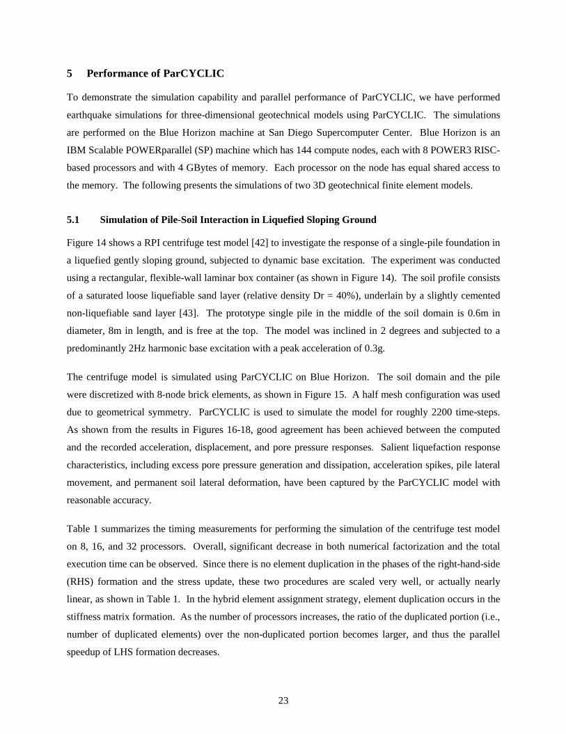
5.1 Simulation of Pile-Soil Interaction in Liquefied Sloping Ground

Figure 14 shows a RPI centrifuge test model [42] to investigate the response of a single-pile foundation in

a liquefied gently sloping ground, subjected to dynamic base excitation. The experiment was conducted

using a rectangular, flexible-wall laminar box container (as shown in Figure 14). The soil profile consists

of a saturated loose liquefiable sand layer (relative density Dr = 40%), underlain by a slightly cemented

non-liquefiable sand layer [43]. The prototype single pile in the middle of the soil domain is 0.6m in

diameter, 8m in length, and is free at the top. The model was inclined in 2 degrees and subjected to a

predominantly 2Hz harmonic base excitation with a peak acceleration of 0.3g.

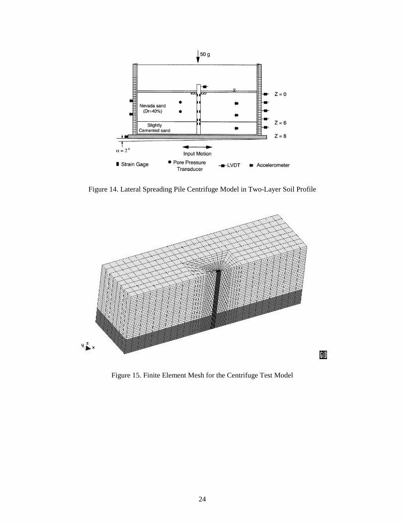
The centrifuge model is simulated using ParCYCLIC on Blue Horizon. The soil domain and the pile

were discretized with 8-node brick elements, as shown in Figure 15. A half mesh configuration was used

due to geometrical symmetry. ParCYCLIC is used to simulate the model for roughly 2200 time-steps.

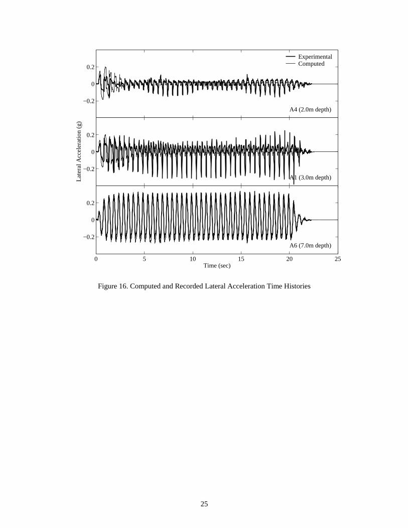
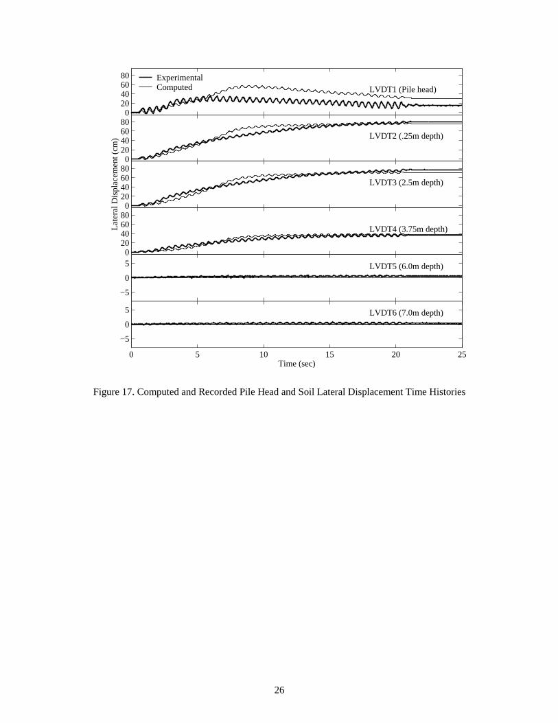
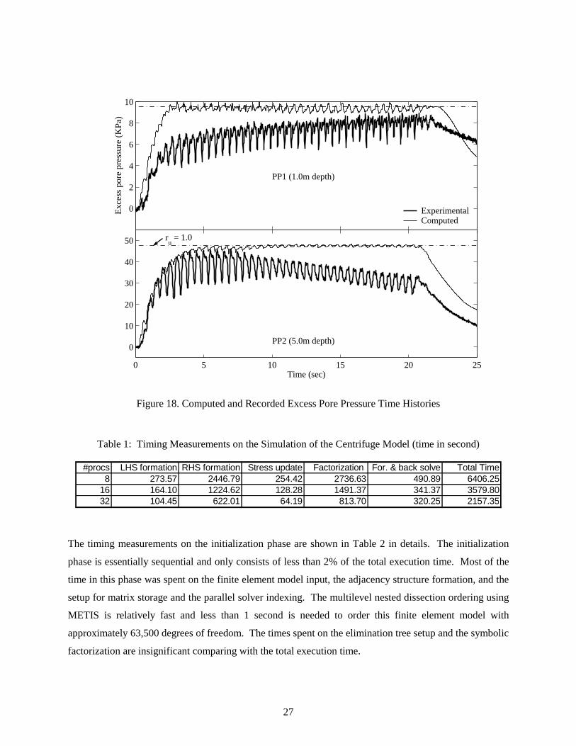
As shown from the results in Figures 16-18, good agreement has been achieved between the computed

and the recorded acceleration, displacement, and pore pressure responses. Salient liquefaction response

characteristics, including excess pore pressure generation and dissipation, acceleration spikes, pile lateral

movement, and permanent soil lateral deformation, have been captured by the ParCYCLIC model with

reasonable accuracy.

Table 1 summarizes the timing measurements for performing the simulation of the centrifuge test model

on 8, 16, and 32 processors. Overall, significant decrease in both numerical factorization and the total

execution time can be observed. Since there is no element duplication in the phases of the right-hand-side

(RHS) formation and the stress update, these two procedures are scaled very well, or actually nearly

linear, as shown in Table 1. In the hybrid element assignment strategy, element duplication occurs in the

stiffness matrix formation. As the number of processors increases, the ratio of the duplicated portion (i.e.,

number of duplicated elements) over the non-duplicated portion becomes larger, and thus the parallel

speedup of LHS formation decreases.

24

Figure 14. Lateral Spreading Pile Centrifuge Model in Two-Layer Soil Profile

Figure 15. Finite Element Mesh for the Centrifuge Test Model

25

−0.2

0

0.2

A4 (2.0m depth)

ExperimentalComputed

−0.2

0

0.2

Late

ral A

ccel

erat

ion

(g)

A1 (3.0m depth)

0 5 10 15 20 25

−0.2

0

0.2

A6 (7.0m depth)

Time (sec)

Figure 16. Computed and Recorded Lateral Acceleration Time Histories

26

020406080

LVDT1 (Pile head)ExperimentalComputed

020406080

LVDT2 (.25m depth)

020406080

Late

ral D

ispl

acem

ent (

cm)

LVDT3 (2.5m depth)

020406080

LVDT4 (3.75m depth)

−5

0

5 LVDT5 (6.0m depth)

0 5 10 15 20 25

−5

0

5 LVDT6 (7.0m depth)

Time (sec)

Figure 17. Computed and Recorded Pile Head and Soil Lateral Displacement Time Histories

27

0

2

4

6

8

10

Exc

ess

pore

pre

ssur

e (K

Pa)

PP1 (1.0m depth)

ExperimentalComputed

0 5 10 15 20 25

0

10

20

30

40

50

PP2 (5.0m depth)

Time (sec)

ru = 1.0

Figure 18. Computed and Recorded Excess Pore Pressure Time Histories

Table 1: Timing Measurements on the Simulation of the Centrifuge Model (time in second)

#procs LHS formation RHS formation Stress update Factorization For. & back solve Total Time8 273.57 2446.79 254.42 2736.63 490.89 6406.25

16 164.10 1224.62 128.28 1491.37 341.37 3579.8032 104.45 622.01 64.19 813.70 320.25 2157.35

The timing measurements on the initialization phase are shown in Table 2 in details. The initialization

phase is essentially sequential and only consists of less than 2% of the total execution time. Most of the

time in this phase was spent on the finite element model input, the adjacency structure formation, and the

setup for matrix storage and the parallel solver indexing. The multilevel nested dissection ordering using

METIS is relatively fast and less than 1 second is needed to order this finite element model with

approximately 63,500 degrees of freedom. The times spent on the elimination tree setup and the symbolic

factorization are insignificant comparing with the total execution time.

28

Table 2. Detailed Timing Results for the Initialization Phase (time in second).

#procs 8 16 32 Finite element mesh read-in 13.18 Adjacency structure formation

9.38

Multilevel nested dissection ordering (using METIS)

0.79

Elimination tree setup and postordering

0.23

Symbolic factorization 1.4

Solver inter-processor communication setup

2.04 3.23 5.19

Matrix storage and solver indexing setup

14.74 9.72 4.11

Total on initialization phase 45 41.78 38.53

5.2 Stone Column Centrifuge Test Model

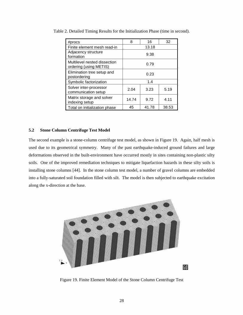
The second example is a stone-column centrifuge test model, as shown in Figure 19. Again, half mesh is

used due to its geometrical symmetry. Many of the past earthquake-induced ground failures and large

deformations observed in the built-environment have occurred mostly in sites containing non-plastic silty

soils. One of the improved remediation techniques to mitigate liquefaction hazards in these silty soils is

installing stone columns [44]. In the stone column test model, a number of gravel columns are embedded

into a fully-saturated soil foundation filled with silt. The model is then subjected to earthquake excitation

along the x-direction at the base.

Figure 19. Finite Element Model of the Stone Column Centrifuge Test

29

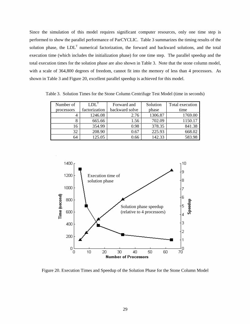
Since the simulation of this model requires significant computer resources, only one time step is

performed to show the parallel performance of ParCYCLIC. Table 3 summarizes the timing results of the

solution phase, the LDLT numerical factorization, the forward and backward solutions, and the total

execution time (which includes the initialization phase) for one time step. The parallel speedup and the

total execution times for the solution phase are also shown in Table 3. Note that the stone column model,

with a scale of 364,800 degrees of freedom, cannot fit into the memory of less than 4 processors. As

shown in Table 3 and Figure 20, excellent parallel speedup is achieved for this model.

Table 3. Solution Times for the Stone Column Centrifuge Test Model (time in seconds)

Number of processors

LDLT factorization

Forward and backward solve

Solution phase

Total execution time

4 1246.08 2.76 1306.87 1769.00 8 665.66 1.56 702.09 1150.17

16 354.99 0.98 378.35 841.38 32 208.90 0.67 225.93 668.02 64 125.05 0.66 142.33 583.98

Figure 20. Execution Times and Speedup of the Solution Phase for the Stone Column Model

Execution time of solution phase

Solution phase speedup (relative to 4 processors)

30

6 Conclusions

This paper presents the analysis and solution strategies employed in ParCYCLIC, a parallel nonlinear

finite element program for the simulations of earthquake site response and liquefaction. In ParCYCLIC,

finite elements are employed within an incremental plasticity, coupled solid-fluid formulation. A

constitutive model developed for the simulation of liquefaction-induced deformations is a main

component of this analysis framework. Extensive calibration of ParCYCLIC has been conducted with

results from experiments and full-scale response of earthquake simulations involving ground liquefaction.

The solution strategy in ParCYCLIC is based on a parallel sparse solver [7]. Several improvements have

been made to the original parallel sparse solver. An automatic domain decomposer is used to partition the

finite element mesh so that the workload on each processor is more or less evenly distributed and the

communication among processors is minimized. METIS routines [33] are incorporated in ParCYCLIC to

perform domain decomposition, and the internal nodes of each sub-domain are ordered using Multilevel

Nested Dissection or other ordering strategies. Because of the automatic domain decomposer, the input

file for ParCYCLIC is very easy to prepare. It does not contain any information for processor assignment

of nodes and elements, and essentially has the same format as the input file for the sequential program

CYCLIC. Moreover, a parallel data structure is introduced to store the matrix coefficients. There are

three different data structures for storing the coefficients of the matrix: one for the principal block

submatrices associated with the column blocks assigned to a single processor, one for the principal block

submatrices associated with column blocks shared by multiple processors, and one for the row segments

in column blocks. An enhancement to the original parallel solver is the processor communication

interface. The original solver is designed for running on Intel supercomputers such as the hypercube, the

Delta system and the Intel Paragon; and the message-passing routines are written using the Intel NX

library [45]. The communication in ParCYCLIC is written in MPI [31]; this makes ParCYCLIC more

portable to run on a wide range of parallel computers and workstation clusters.

Large-scale experimental results for 3-D geotechnical simulations have been presented to demonstrate the

capability and performance of ParCYCLIC. Simulation results demonstrated that ParCYCLIC is suitable

for large-scale geotechnical simulations, and good agreement has been achieved between the computed

and the recorded acceleration, displacement, and pore pressure responses. Excellent parallel speedup has

also been obtained from the simulation results. Last but not least, it is shown that ParCYCLIC program,

which employs direct solution scheme, remains scalable to a large number of processors, e.g., 64 or more.

31

Acknowledgements

This research was supported in part by the National Science Foundation, Grant Number CMS-0084616 to

University of California, San Diego, and Grant Number CMS-0084530 to Stanford University.

Additional funding was provided in part by the Pacific Earthquake Engineering Research (PEER) Center,

under the National Science Foundation Award Number EEC-9701568. Thanks to Dr. Zhaohui Yang at

University of California, San Diego for his assistance with the development of the original CYCLIC

program. This research was also supported in part by NSF cooperative agreement ACI-9619020 through

computing resources provided by the National Partnership for Advanced Computational Infrastructure at

the San Diego Supercomputer Center.

References

1. Gummadi LNB, Palazotto AH. Nonlinear finite element analysis of beams and arches using parallel processors. Computers and Structures 1997; 63:413-428.

2. Amestoy PR, Duff IS, L'Excellent J-Y. Multifrontal parallel distributed symmetric and unsymmetric solvers. Computer Methods in Applied Mechanics and Engineering 2000; 184(2-4):501-520.

3. Li XS, Demmel JW. Making sparse Gaussian elimination scalable by static pivoting. Proceedings of SC98: High Performance Networking and Computing Conference. Orlando, FL, 1998.

4. Heath MT, Ng E, Peyton BW. Parallel algorithms for sparse linear systems. SIAM Review 1991; 33(3):420-460.

5. George A, Heath MT, Liu J, Ng E. Solution of sparse positive definite systems on a shared-memory multiprocessor. International Journal of Parallel Programming 1986; 15(4):309-328.

6. George A, Heath MT, Liu J, Ng E. Solution of sparse positive definite systems on a hypercube. Journal of Computational and Applied Mathematics 1989; 27(1-2):129-156.

7. Law KH, Mackay DR. A parallel row-oriented sparse solution method for finite element structural analysis. International Journal for Numerical Methods in Engineering 1993; 36(17):2895-2919.

8. Watson BC, Noor AK. Nonlinear structural analysis on distributed-memory computers. Computers and Structures 1996; 58(2):233-247.

9. Nikishkov GP, Kawka M, Makinouchi A, Yagawa G, Yoshimura S. Porting an industrial sheet metal forming code to a distributed memory parallel computer. Computers and Structures 1998; 67(6):439-449.

10. Romero ML, Miguel PF, Cano JJ. A parallel procedure for nonlinear analysis of reinforced concrete three-dimensional frames. Computers and Structures 2002; 80(16-17):1337-1350.

11. Modak S, Sotelino ED. An object-oriented programming framework for the parallel dynamic analysis of structures. Computers and Structures 2002; 80(1):77-84.

12. McKenna F. Object-oriented finite element programming: Frameworks for analysis, algorithm and parallel computing. Ph.D. Thesis, University of California at Berkeley, Berkeley, CA 1997.

32

13. Krysl P, Bittnar Z. Parallel explicit finite element solid dynamics with domain decomposition and message passing: Dual partitioning scalability. Computers and Structures 2001; 79(3):345-360.

14. Bao H, Bielak J, Ghattas O, O'Hallaron DR, Kallivokas LF, Shewchuk JR, Xu J. Earthquake ground motion modeling on parallel computers. Proceedings of ACM/IEEE Supercomputing Conference. Pittsburgh, PA, 1996.

15. Parra E. Numerical modeling of liquefaction and lateral ground deformation including cyclic mobility and dilation response in soil systems. Ph.D. Thesis, Rensselaer Polytechnic Institute, Troy, NY 1996.

16. Yang Z, Elgamal A. Influence of permeability on liquefaction-induced shear deformation. Journal of Engineering Mechanics, ASCE 2002; 128(7):720-729.

17. Chan AHC. A unified finite element solution to static and dynamic problems in geomechanics. Ph.D. Thesis, University of Wales, Swansea, U.K. 1988.

18. Zienkiewicz OC, Chan AHC, Pastor M, Paul DK, Shiomi T. Static and dynamic behavior of soils: A rational approach to quantitative solutions: I. Fully saturated problems. Proceedings of the Royal Society London, Series A, Mathematical and Physical Sciences 1990; 429:285-309.

19. Yang Z. Numerical modeling of earthquake site response including dilation and liquefaction. Ph.D. Thesis, Columbia University, New York, NY 2000.

20. Biot MA. The mechanics of deformation and acoustic propagation in porous media. Journal of Applied Physics 1962; 33(4):1482-1498.

21. Elgamal A, Yang Z, Parra E, Ragheb A. Modeling of cyclic mobility in saturated cohesionless soils. International Journal of Plasticity 2003; 19(6):883-905.

22. Prevost JH. A simple plasticity theory for frictional cohesionless soils. International Journal of Soil Dynamics and Earthquake Engineering 1985; 4(1):9-17.

23. Elgamal A, Yang Z, Parra E. Computational modeling of cyclic mobility and post-liquefaction site response. Journal of Soil Dynamics and Earthquake Engineering 2002; 22(4):259-271.

24. Elgamal A, Parra E, Yang Z, Adalier K. Numerical analysis of embankment foundation liquefaction countermeasures. Journal of Earthquake Engineering 2002; 6(4):447-471.

25. Ishihara K, Tatsuoka F, Yasua S. Undrained deformation and liquefaction of sand under cyclic stresses. Soils and Foundations 1975; 15(1):29-44.

26. Mroz Z. On the description of anisotropic work hardening. Journal of Mechanics and Physics of Solids 1967; 15(1):163-175.

27. Mackay DR. Solution methods for static and dynamic structural analysis on distributed memory computers. Ph.D. Thesis, Stanford University, Stanford, CA 1992.

28. Herndon B, Aluru N, Raefsky A, Goossens RJG, Law KH, Dutton RW. A methodology for parallelizing pde solvers: Applications to semiconductor device simulation. Proceedings of the Seventh SIAM Conference on Parallel Processing for Scientific Computing. San Francisco, CA, 1995.

29. Law KH. Large scale engineering computations on distributed memory parallel computers and distributed workstations. Proceedings of NSF Workshop on Scientific Supercomputing, Visualization and Animation in Geotechnical Earthquake Engineering and Engineering Seismology. Carnegie-Mellon University, Pittsburgh, PA, 1994.

30. Aluru NR. Parallel and stabilized finite element methods for the hydrodynamic transport model of semiconductor devices. Ph.D. Thesis, Stanford University, Stanford, CA 1995.

33

31. Snir M, Gropp W. MPI: The complete reference. MIT Press: Boston, MA, 1998.

32. Fahmy MW, Namini AH. A survey of parallel nonlinear dynamic analysis methodologies. Computers and Structures 1994; 53(4):1033-1043.

33. Karypis G, Kumar V. METIS version 4.0: A software package for partitioning unstructured graphs, partitioning meshes, and computing fill-reducing orderings of sparse matrices. Department of Computer Science and Engineering, University of Minnesota, 1998

34. Karypis G, Kumar V. A fast and high quality multilevel scheme for partitioning irregular graphs. SIAM Journal on Scientific Computing 1998; 20(1):359-392.

35. Karypis G, Kumar V. Multilevel k-way partitioning scheme for irregular graphs. Journal for Parallel and Distributed Computing 1998; 48(1):96-129.

36. George A. Computer implementation of the finite element method. Ph.D. Thesis, Stanford University, Stanford, CA 1971.

37. Tinney WF, Walker JW. Direct solutions of sparse network equations by optimally ordered triangular factorization. Proceedings of the IEEE 1967; 55(11):1801-1809.

38. Lipton RJ, Rose DJ, Tarjan RE. Generalized nested dissection. SIAM Journal on Numerical Analysis 1979; 16(1):346-358.

39. Liu JWH. The role of elimination trees in sparse factorization. SIAM Journal on Matrix Analysis and Applications 1990; 11(1):134-172.

40. Law KH, Fenves SJ. A node-addition model for symbolic factorization. ACM Transactions on Mathematical Software 1986; 12(1):37-50.

41. Liu JWH. A generalized envelope method for sparse factorization by rows. ACM Transactions on Mathematical Software 1991; 17(1):112-129.

42. Abdoun T. Modeling of seismically induced lateral spreading of multi-layered soil and its effect on pile foundations. Ph.D. Thesis, Rensselaer Polytechnic Institute, Troy, NY 1997.

43. Abdoun T, Doubry R. Evaluation of pile foundation response to lateral spreading. Soil Dynamics and Earthquake Engineering 2002; 22(9-12):1069-1076.

44. Pekcan G, Yen WP, Friedland IM. Seismic vulnerability study of highway systems: Tea-21 research project. Proceedings of 15th U.S.-Japan Bridge Engineering Workshop. Tsukuba, Japan, 1999.

45. Pierce P, Regnier G. The paragon implementation of the NX message passing interface. Proceedings of the Scalable High Performance Computing Conference (SHPCC94). Knoxville, TN, 1994.