Parity violation in electron scattering - Home - Springer · 2.6.3 Higher twist 10 ... 4.2.4 SUSY 25 c The Author(s) 2015 ... the ﬁrst observation of parity violation in electron

Front. Phys. 11(1), 111301 (2016)

DOI 10.1007/s11467-015-0482-0

REVIEW ARTICLE

Parity violation in electron scattering

P. Souder1,†, K. D. Paschke2

1Syracuse University, Syracuse, NY 13244, USA

2University of Virginia, Charlottesville, VA 22904, USA

Corresponding author. E-mail: †[email protected]

Received August 31, 2015; accepted September 25, 2015

By comparing the cross sections for left- and right-handed electrons scattered from various unpolar-ized nuclear targets, the small parity-violating asymmetry can be measured. These asymmetry dataprobe a wide variety of important topics, including searches for new fundamental interactions andimportant features of nuclear structure that cannot be studied with other probes. A special featureof these experiments is that the results are interpreted with remarkably few theoretical uncertain-ties, which justifies pushing the experiments to the highest possible precision. To measure the smallasymmetries accurately, a number of novel experimental techniques have been developed.

Keywords weak neutral currents, weak form factors, parton distributions, neutron stars, physicsbeyond the standard model

PACS numbers 11.30.Er, 13.40.GP, 24.80.+y, 25.30.Bf

Contents

1 Introduction 21.1 History of the field 21.2 Experimental overview 31.3 Neutrino scattering and PVES 41.4 Atomic parity violation 41.5 Theory of parity violation in potential

scattering 41.6 More realistic cases 51.7 Precision of SM predictions 6

1.7.1 Higher-order corrections 61.7.2 Uncertainties in radiative corrections 61.7.3 Experimental implications 6

2 Theory 62.1 Kinematics 62.2 Phenomenology 72.3 Weak charges 72.4 Strange form factors 82.5 Radius of neutron distribution 92.6 Parity violation in deep inelastic scattering 9

2.6.1 PVDIS for deuterium 102.6.2 Charge symmetry 102.6.3 Higher twist 102.6.4 PVDIS with a proton target 10

2.7 Møller scattering 11

∗Special Topic: Spin Physics (Eds. Haiyan Gao & Bo-Qiang Ma).

3 Experimental details 113.1 Rates and statistical errors 113.2 Accelerators 123.3 Polarized beam 123.4 Helicity-correlated changes in the beam 123.5 Slow helicity reversals 133.6 Targets 143.7 Spectrometers 14

3.7.1 JLab high-resolution spectrometer 163.7.2 G0 toroidal spectrometer 163.7.3 Crystal spectrometer at Mainz 173.7.4 The Qweak spectrometer 183.7.5 JLab SoLID spectrometer 18

3.8 Møller spectrometers 183.9 Detectors 19

3.9.1 Integrating detectors 193.9.2 Counting detectors 20

3.10 Electronics 203.11 Polarimetry 20

3.11.1 Møller polarimeters 203.11.2 Compton polarimeters 21

3.12 Q2 calibration 214 Results and implications 22

4.1 Strange form factors 224.2 Electroweak tests 22

4.2.1 Limits on compositeness 244.2.2 Leptophobic Z ′ boson 244.2.3 Dark light 254.2.4 SUSY 25

c© The Author(s) 2015. This article is published with open access at www.springer.com/11467 and journal.hep.com.cn/fop

REVIEW ARTICLE

4.3 Radius of neutron distributions 255 Summary and conclusions 27

Acknowledgements 27References 27

1 Introduction

Electron scattering has proven to be an important toolfor exploring the structure of nuclei and the nucleonsfrom which they are made. Highlights include the deter-mination of the precise sizes and shapes of many differentnuclei [1] and the discovery that nucleons are composedof electrically charged point-like particles, which are nowknown as quarks [2, 3].

Ultimately, electron scattering from nuclei is due tothe electromagnetic interaction of the electrons with thequarks: up quarks with a charge of 2/3 and down quarkswith charge −1/3 (as well as strange quarks). The elec-tromagnetic interaction is relatively weak and can be de-scribed accurately as the exchange of a single photon.Consequently, electron scattering data are straightfor-ward to interpret theoretically.

In this review, we describe the field of parity viola-tion in electron scattering (PVES), in which the quantitymeasured is

APV = −ALR =σR − σL

σR + σL, (1)

where σR (σL) is the cross section for the scattering ofelectrons with right (left) helicity. Because electromag-netism conserves parity, any nonzero value of APV mustbe due to the weak interaction through exchange of theZ boson in the Standard Model (SM) or to new physicsbeyond the SM (BSM). Measuring an asymmetry hasa number of advantages, including the cancellation ofmany possible theoretical and experimental uncertain-ties.

There are three motivations for this program:

1) To measure the parameters of the SM, especiallythe couplings of the Z boson [4];

2) To search for new parity-violating interactions(BSM physics) [5];

3) To measure properties of nuclei that cannot bestudied accurately with other probes [6].

The advantages of PVES for the first two points areevident. For studying nuclei, PVES has the advantagethat the quarks have different charges when interactingwith the Z boson instead of the photon. For the Z bo-son, the charge of the neutron is much larger than thatof the proton, in striking contrast to the nucleon charges

for photon exchange. Thus, PVES is sensitive to the dis-tribution of the neutrons in a nucleus, in contrast tounpolarized electron scattering, which is sensitive to thedistribution of the protons.

1.1 History of the field

In the common decays of radioactive nuclei into elec-trons and neutrinos, weak currents are observed thatcarry charge. In 1958, Wu et al. [7] found that thesecharged weak currents violated parity. In the 1970s, neu-trinos were observed to interact with matter without pro-ducing electrons or muons, proving that there are alsoneutral weak currents. One of the theories at the time,now called the Standard Model, predicted that the neu-tral current would also violate parity. However, publishedexperiments on atomic parity violation (APV) suggestedthat parity violation was much smaller than predicted bythe SM. In 1978, the first observation of parity violationin electron scattering was published by Prescott et al. [8,9] and helped lead to a general acceptance of the SM.These observations marked the beginning of the field ofPVES.

The Prescott experiment was challenging because theasymmetry measured was only 10−4, a tiny fraction ofthe cross section. To achieve this feat, the experimentrequired a number of experimental innovations, many ofwhich are still central to the field of PVES today. Perhapsthe most important is the development of a polarizedelectron source based on photoemission from GaAs. Thesource featured high intensity and the ability to reversethe helicity of the beam without making large changesin the beam properties such as the position, angle, orenergy. To verify that the beam was almost perfectly re-versed, a set of precision beam monitors was developed.Finally, the signals from the scattering events were in-tegrated rather than counted, as was the practice forvirtually all particle physics experiments. Integrating thesignals allowed accumulation of the large statistics neces-sary for measuring the small parity-violating asymmetry.

The Prescott experiment was followed by two PVESexperiments using nuclei as targets. Both experiments[10, 11], which were designed to test the predictions ofthe SM, were able to measure even smaller asymmetries.In addition to confirming the predictions of the SM, theseefforts demonstrated the power of PVES as a generaltool. We will refer to these experiments as Generation IPVES experiments.

The advent of the “spin crisis” in 1989 [12, 13], inwhich data on the spin-structure functions of the pro-ton indicated that the spin of the proton was not sim-ply the sum of the spins of the valence quarks, raised

111301-2 P. Souder and K. D. Paschke, Front. Phys. 11(1), 111301 (2016)

REVIEW ARTICLE

the question of the role of strange quarks in the nucleon[14]. McKeown [15] explained that PVES was a practicalway to measure the strangeness content of nucleon elas-tic form factors. Four experimental programs in threelaboratories, the Generation II PVES experiments, fol-lowed. The experiments were SAMPLE at the MIT Bateslaboratory [16–18], the HAPPEX program at JLab [19–21], G0 at JLab [22, 23], and the A4 program at Mainz[24–26]. By the time these programs were well underway,PVES had become accepted as a standard technique inelectromagnetic facilities.

The success of the strange-form-factor program led tothe publication of some even more challenging experi-ments providing improved SM tests, SLAC E158 [27] andQweak [28] at JLab and also the JLab PREx experiment[29], which measured PVES on 208Pb to determine thecharge radius of the neutron distribution. These, alongwith the future PREx-II and CREx measurements, arethe Generation III PVES experiments.

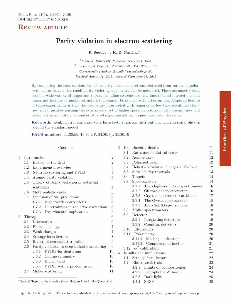
A number of even more challenging Generation IVPVES experiments have been proposed, of which theP2 experiment at Mainz [30] and the MOLLER [31]and SoLID experiments at JLab have been approved.These experiments will push the limits regarding bothhow small an asymmetry can be measured and howprecisely that asymmetry can be measured. The preci-sion of the various PVES experiments is summarized inFig. 1.

1.2 Experimental overview

In a typical PVES experiment, a beam of electrons with

Fig. 1 Summary of past and future PVES measurements. Hori-zontal axis: measured value of the asymmetry APV . Vertical axis:total experimental error. The diagonal lines indicate the fractionalerror in the asymmetry measurements.

energy E scatters from the target at an angle θ andemerges with energy E′. No other particles are detected;the process is called inclusive scattering. The cross sec-tion and asymmetry depend mainly on two parameters,the magnitude of the four-momentum transfer,

Q2 = 4EE′ sin2 θ/2, (2)

and the electron energy loss ν,

ν = E − E′. (3)

For elastic scattering events, in which no other particlesare produced,

Q2 = 2Mν, (4)

where M is the mass of the target. Inelastic events canbe identified by the fact that E′ is less than that pre-dicted by Eq. (4).

The quantity APV is typically less that 10−4Q2

(GeV/c)−2, where Q2 for PVES experiments ranges from0.01 to 10 (GeV/c)2. For lower Q2 values, the mea-sured asymmetries are quite small, often well below 1part per million (ppm), and very high rates are requiredto make measurements with sufficient statistics. In addi-tion, great care must be taken when reversing the helicityto preserve the properties of the beam. Any systematicdifference in the position, angle, or energy of beams ofdifferent helicity can cause a difference in the measuredrate that has nothing to do with parity violation. Fortu-nately, the helicity of electron beams can be rapidly andcleanly reversed, typically at rates greater than 1 kHz.Slow drifts in the efficiency of the apparatus are thuseliminated, and many systematic errors that are impor-tant for cross section measurements, such as the targetthickness and angular acceptance of the scattered elec-tron, cancel in the asymmetry. A remarkable precisioncan be achieved in PVES experiments; sensitivities assmall as 20 parts per billion (ppb) have been published,and planned experiments are expected to achieve sensi-tivities below the ppb level.

Elastic scattering is ideal for PVES experiments. Atlow Q2 values, the cross section is large, so large statis-tics can be obtained. In addition, only the highest-energyelectrons represent elastic scattering. These electrons canbe cleanly identified using a magnetic spectrometer orcalorimeter and distinguished from the lower-energy elec-trons from inelastic background processes.

The experimental facilities designed to measure elec-tromagnetic cross sections were also found to be suit-able for PVES experiments, even though the data ratesfor the two types of experiments differ by many ordersof magnitude. The experiments are compatible becauseimportant cross sections for some scattering angles are

P. Souder and K. D. Paschke, Front. Phys. 11(1), 111301 (2016) 111301-3

REVIEW ARTICLE

highly suppressed by the form factors (see the next sec-tion), and the facilities were designed to measure theseextremely small cross sections. When the same appara-tus is used for reactions with large cross sections, thestatistics required for PVES become available. However,new detector and data acquisition (DAQ) systems arerequired to handle the higher rates.

1.3 Neutrino scattering and PVES

Neutrino scattering provides an alternative method ofmeasuring the interaction of the Z boson with electronsor nuclei. There are a number of important differencesbetween the two processes, both theoretical and experi-mental:

1) The neutrino has no vector charge.2) Neutrino scattering has contributions from terms

with both gt and gb purely axial. These terms donot contribute to APV .

3) The radiative corrections are different and in somecases are smaller for neutrinos than for electrons.

4) The energy of the incoming neutrino beam cannotbe precisely known, and the scattered neutrino can-not be detected. This reduces the knowledge of in-dividual events. Thus, the data are usually summedover large bins in Q2 and ν, washing out some ofthe important physics.

An extensive literature on this subject exists [32]. Oneneutrino experiment, however, is especially relevant forPVES. The NuTeV collaboration [33] published a resultbased on deep inelastic scattering (DIS) with neutrinosthat disagrees with the SM. There is an ongoing debateabout the interpretation of this result.

1.4 Atomic parity violation

A probe complementary to PVES is APV. A parity-violating interaction between the electrons and nucleusin an atom can allow atomic transitions that otherwiseare forbidden. A particularly precise experiment on APVin Cs has been published [34]. (The interpretation of thatresult depends on calculations of the atomic wave func-tions that have improved since the publication of theresult, as discussed in Ref. [4].)

Even more precise APV experiments may be feasiblein the future, for example, with trapped Ra ions [35]. Theinformation obtained by APV is very similar to that ob-tained by elastic scattering from light N + Z nuclei atlow Q2.

1.5 Theory of parity violation in potential scattering

To explain the main features of PVES, we will describea case that is easy to calculate, namely, nonrelativis-tic potential scattering [36]. Let a spherical nucleus becomposed of N charged objects that have a numberdensity distribution ρ(r). The distribution ρ(r) can beeither a classical charge distribution or, for a realisticnucleus, a quantum mechanical probability distribution.The Fourier transform of the number distribution, whichis called the form factor, is defined as

F (Q2) ≡∫

ρ(r) exp(iq · r)d3r, (5)

where q is the momentum transfer, which is the differ-ence between the momenta of the incident and scatteredelectrons. Clearly

F (0) =∫

ρ(r)d3r = N. (6)

The potential for weak or electromagnetic scatteringcan be expressed by the formula

V (r) = ke2gbgt exp(−Mr)4πr

,

where M is the mass of the exchanged particle, k is acoupling constant, and gb and gt are the charges of thebeam and target particles, respectively, in units of e. Forelectromagnetic electron scattering, which involves pho-ton exchange, M = 0, k = 1, gt = qt

EM , and gb = −1.For the weak interaction, which involves Z exchange,M = MZ = 91 GeV, and k = kZ = (sin θW cos θW )−2.Here e2 = 4πα.

For Z exchange, the couplings of gb and gt dependon the helicity of the particle, resulting in the parity-violating asymmetry APV . Values of the helicity differ-ence in gb for Z exchange (gA ≡ gL − gR) are givenin Table 1. For quarks in a nucleus with no angular mo-mentum, the scattering depends only on the average cou-pling gt

V ≡ (gtR+gt

L)/2. However, for polarized electrons,the coupling is different for different helicities. The weakcharges are also given in Table 1.

The scattering amplitude in the Born approximationis

fL(R)(Q2) =2kmαgb

L(R)

Q2 + M2gtF (Q2), (7)

where m is the mass of the electron. The same form fac-tor arises for both weak and electromagnetic scattering,even though the ranges of the two interactions are to-tally different. Because both weak and electromagneticscattering are coherent, the total scattering amplitude is


REVIEW ARTICLE

Table 1 Weak and electromagnetic charges for electrons, lightquarks, and the nucleons in units of the electron charge e.

Particle qEM gV gA

e− −1 − 12

+ 2 sin2 θW12

u 23

12− 4

3sin2 θW − 1

2

d, s − 13

− 12

+ 23

sin2 θW12

p 1 12− 2 sin2 θW − 1

2

n 0 − 12

12

fL(R)Total(Q

2) = fγ + fL(R)Z

=

(−qt

EM

Q2+

kZgbL(R)g

tV

M2Z

)2mαF (Q2).

The scattering cross section is proportional to the squareof the amplitude and hence proportional to F (Q2)2. Thesizes and shapes of nuclei have been determined by mea-suring the cross section, and hence F (Q2), over a broadrange of Q2 and inverting the Fourier transform of Eq.(5). Because M2

Z � Q2, the fγ term dominates the de-nominator of APV but is canceled in the numerator,where the interference term fγfZ dominates.

Thus,

APV = −fγ(fRZ − fL

Z )f2

γ

=fL

Z − fRZ

fγ=

Q2kZgbAgt

V

qtEMM2

Z

.

(8)

The result is quite remarkable. The form factor is can-celed, and ALR is linear in Q2, with a slope that de-pends only on the fundamental parameters of the SM.This follows from Eq. (7). The scattering amplitude isproportional to F (Q2), regardless of the value of M orthe charges.

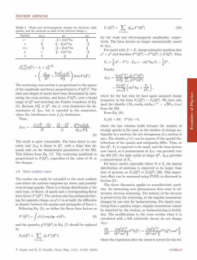
1.6 More realistic cases

The results can easily be extended to the more realisticcase where the nucleus comprises up, down, and possiblyeven strange quarks. There is a charge distribution ρi foreach type, or flavor, of quark and a corresponding flavorform factor F i(Q2). The nucleus also has antiquarks hav-ing the opposite charge, so ρi(r) is actually the differencein density between the quarks and antiquarks of flavor i.

Following Eq. (5), we define the flavor form factors as

F i(Q2) =∫

ρi(r) exp(iq · r)d3r, (9)

and the quantity gtF (Q2) in Eq. (7) should be replacedby

FZ(Q2) =∑

i=u,d,s

giV F i(Q2);

Fγ(Q2) =∑

i=u,d,s

qiEMF i(Q2) (10)

for the weak and electromagnetic amplitudes, respec-tively. The form factors no longer automatically cancelin APV .

For nuclei with N = Z, charge symmetry predicts thatρu = ρd and therefore Fu(Q2) = F d(Q2) ≡ F (Q2). Then

Fγ =13(F − F s); FZ = − sin2 θW Fγ − 1

4F s.

Finally,

APV =kZQ2

2M2Z

∑i gi

V F i(Q2)∑i qiF i(Q2)

→ GF Q2

πα√

2

(sin2 θW +

Fs

4Fγ

),

where for the last step we have again assumed chargesymmetry in the form Fu(Q2) = Fd(Q2). We have alsoused the identity (MZ cos θW sin θW )−2 =

√2GF /(πα)

from the SM.From Eq. (6),

Fγ(0) = 3Z; F s(0) = 0,

where the last relation holds because the number ofstrange quarks is the same as the number of strange an-tiquarks in a nucleus; the net strangeness of a nucleus iszero. The density ρs(r) can be nonzero if the spatial dis-tributions of the quarks and antiquarks differ. Thus, atlow Q2, Fs is expected to be small, and the form factorsnow cancel, so a measurement of APV can precisely testthe SM [37]. For light nuclei at larger Q2, ALR providesa measurement of Fs.

For heavy nuclei, especially where N �= Z, the spatialdistribution of neutrons is expected to be larger thanthat of protons, so Fu(Q2) �= Fd(Q2) [38]. This impor-tant effect can be measured using PVES, as discussed inSection 2.5.

The above discussion applies to nonrelativistic parti-cles. An interesting new phenomenon does arise in rel-ativistic electron scattering. The helicity of the electronis preserved in the scattering, so the angular momentumchanges by one unit for backscattering. For elastic scat-tering from a spinless target, angular momentum cannotbe absorbed by the nucleus, so backscattering is forbid-den. The modifications to the cross section when it iscalculated with a full relativistic theory do not changeAPV :

dσ

dΩ=

(αgbgt)2

4E2 sin4 θ2

F 2(Q2) → (αgbgt)2

4E2 sin4 θ2

F 2(Q2) cos2θ

2,

where the expression after the arrow is correct for the rel-


REVIEW ARTICLE

ativistic case. The only change is the factor of cos2 θ/2.For scattering from a target with spin, such as the pro-

ton, backscattering is allowed, and the spin of the tar-get is flipped. Targets with spin also have magnetic mo-ments, and the resulting magnetic fields contribute ap-preciably to the scattering, especially at large angles. Inaddition, backscattered electrons can scatter only fromquarks with opposite helicity in the center-of-mass (CM)frame. Thus, in this case the axial charge of the quarkscontributes to the asymmetry. These features appear inthe detailed formulae in Section 2.

1.7 Precision of SM predictions

One of the beauties of the SM is that it makes manypredictions with spectacular precision. The SM requiresonly three parameters as input; the typical choice is α,GF from muon decay, and MZ from collider experiments.These parameters are now known to very high accuracy.The SM is in fact a perturbation theory with a small cou-pling constant α/2π ∼ 10−3; hence, the first-order ap-proximations, called tree-level predictions, are expectedto be accurate to the 0.1% level. Furthermore, the SM isa renormalizable theory. This means that, in principle,these higher-order corrections can be made to any orderand with arbitrary precision.

1.7.1 Higher-order corrections

One problem with the SM is that the higher-order cor-rections, called radiative corrections, are in fact muchlarger than would be expected on the basis of the smallcoupling constant. There are two main reasons for this.

The first arises from the fact that the SM unifiesphysics over a striking breadth of the energy scale.Hadrons in the theory have structure at the 100 MeVscale, whereas the mass of the Z is nearly 100 GeV.A quark isodoublet, the b and t quarks, has a massdifference well in excess of 100 GeV. Recent precisemeasurements of the top quark mass and also the dis-covery of the Higgs particle and determination of itsmass have further reduced the uncertainties in the ra-diative corrections. These large energy differences givelarge logarithms that enhance the radiative correctionsfrom the naive level of 0.1% to about 5%. (The precisecalculation of these radiative corrections requires knowl-edge of the quark masses and the Higgs mass, in additionto the three parameters mentioned above.) The secondfeature that makes the radiative corrections large is thatalthough the vector charges of unit charge particles aremuch smaller than the axial charges, radiative correctionwith a vector charge often involves an axial charge, thus

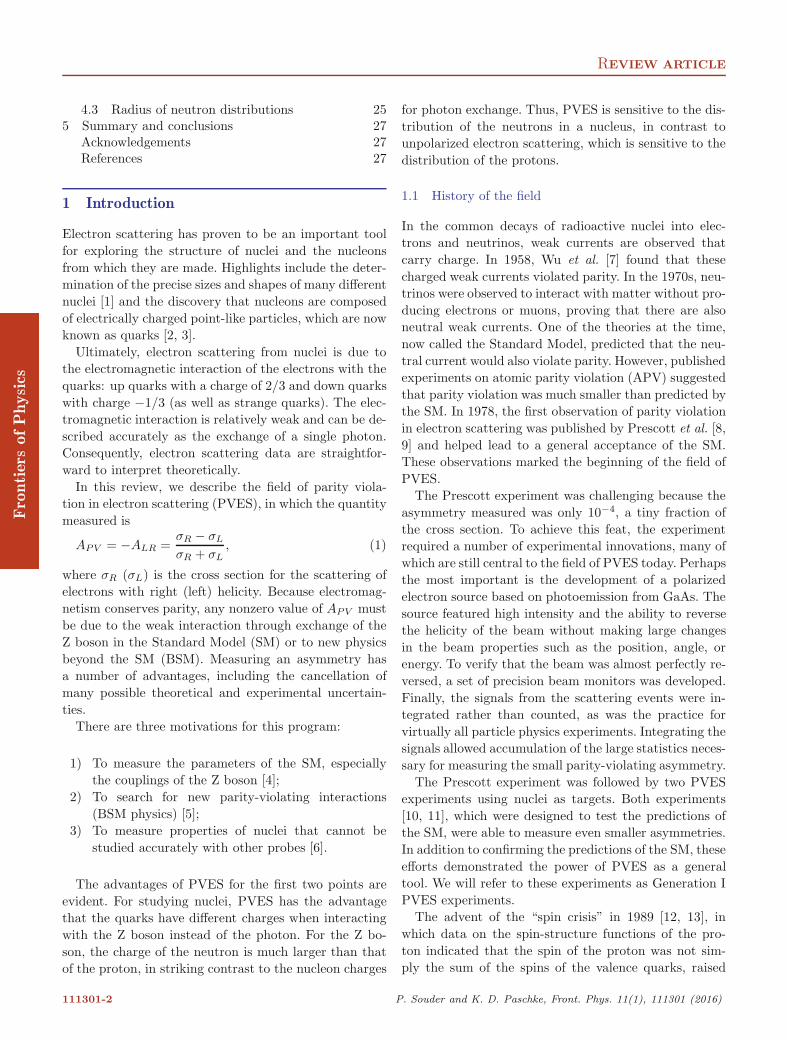
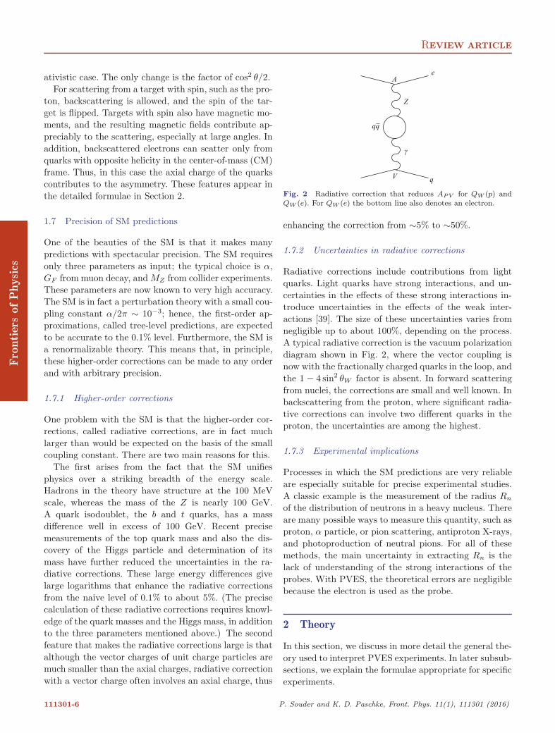
Fig. 2 Radiative correction that reduces APV for QW (p) andQW (e). For QW (e) the bottom line also denotes an electron.

enhancing the correction from ∼5% to ∼50%.

1.7.2 Uncertainties in radiative corrections

Radiative corrections include contributions from lightquarks. Light quarks have strong interactions, and un-certainties in the effects of these strong interactions in-troduce uncertainties in the effects of the weak inter-actions [39]. The size of these uncertainties varies fromnegligible up to about 100%, depending on the process.A typical radiative correction is the vacuum polarizationdiagram shown in Fig. 2, where the vector coupling isnow with the fractionally charged quarks in the loop, andthe 1 − 4 sin2 θW factor is absent. In forward scatteringfrom nuclei, the corrections are small and well known. Inbackscattering from the proton, where significant radia-tive corrections can involve two different quarks in theproton, the uncertainties are among the highest.

1.7.3 Experimental implications

Processes in which the SM predictions are very reliableare especially suitable for precise experimental studies.A classic example is the measurement of the radius Rn

of the distribution of neutrons in a heavy nucleus. Thereare many possible ways to measure this quantity, such asproton, α particle, or pion scattering, antiproton X-rays,and photoproduction of neutral pions. For all of thesemethods, the main uncertainty in extracting Rn is thelack of understanding of the strong interactions of theprobes. With PVES, the theoretical errors are negligiblebecause the electron is used as the probe.

2 Theory

In this section, we discuss in more detail the general the-ory used to interpret PVES experiments. In later subsub-sections, we explain the formulae appropriate for specificexperiments.


REVIEW ARTICLE

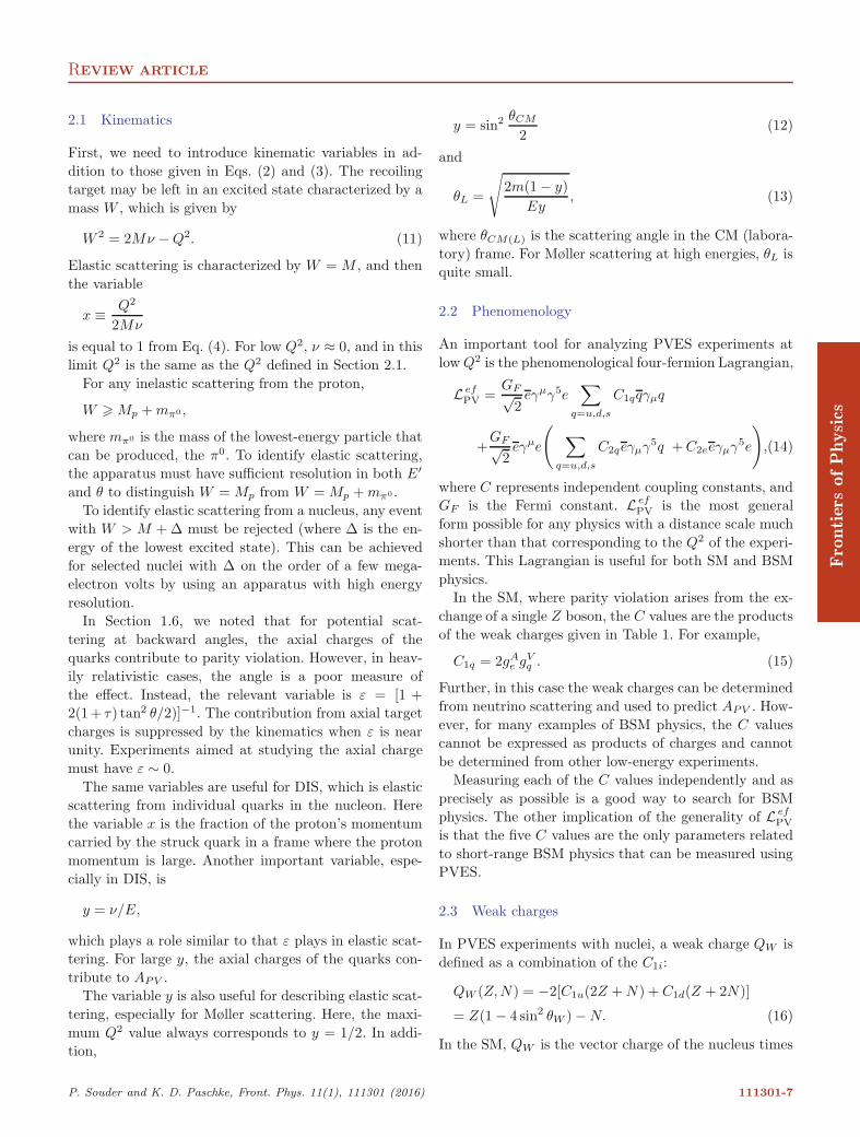
2.1 Kinematics

First, we need to introduce kinematic variables in ad-dition to those given in Eqs. (2) and (3). The recoilingtarget may be left in an excited state characterized by amass W , which is given by

W 2 = 2Mν − Q2. (11)

Elastic scattering is characterized by W = M , and thenthe variable

x ≡ Q2

2Mν

is equal to 1 from Eq. (4). For low Q2, ν ≈ 0, and in thislimit Q2 is the same as the Q2 defined in Section 2.1.

For any inelastic scattering from the proton,

W � Mp + mπ0 ,

where mπ0 is the mass of the lowest-energy particle thatcan be produced, the π0. To identify elastic scattering,the apparatus must have sufficient resolution in both E′

and θ to distinguish W = Mp from W = Mp + mπ0 .To identify elastic scattering from a nucleus, any event

with W > M + Δ must be rejected (where Δ is the en-ergy of the lowest excited state). This can be achievedfor selected nuclei with Δ on the order of a few mega-electron volts by using an apparatus with high energyresolution.

In Section 1.6, we noted that for potential scat-tering at backward angles, the axial charges of thequarks contribute to parity violation. However, in heav-ily relativistic cases, the angle is a poor measure ofthe effect. Instead, the relevant variable is ε = [1 +2(1+ τ) tan2 θ/2)]−1. The contribution from axial targetcharges is suppressed by the kinematics when ε is nearunity. Experiments aimed at studying the axial chargemust have ε ∼ 0.

The same variables are useful for DIS, which is elasticscattering from individual quarks in the nucleon. Herethe variable x is the fraction of the proton’s momentumcarried by the struck quark in a frame where the protonmomentum is large. Another important variable, espe-cially in DIS, is

y = ν/E,

which plays a role similar to that ε plays in elastic scat-tering. For large y, the axial charges of the quarks con-tribute to APV .

The variable y is also useful for describing elastic scat-tering, especially for Møller scattering. Here, the maxi-mum Q2 value always corresponds to y = 1/2. In addi-tion,

y = sin2 θCM

2(12)

and

θL =

√2m(1 − y)

Ey, (13)

where θCM(L) is the scattering angle in the CM (labora-tory) frame. For Møller scattering at high energies, θL isquite small.

2.2 Phenomenology

An important tool for analyzing PVES experiments atlow Q2 is the phenomenological four-fermion Lagrangian,

L efPV =

GF√2

eγμγ5e∑

q=u,d,s

C1qqγμq

+GF√

2eγμe

( ∑q=u,d,s

C2qeγμγ5q + C2eeγμγ5e

),(14)

where C represents independent coupling constants, andGF is the Fermi constant. L ef

PV is the most generalform possible for any physics with a distance scale muchshorter than that corresponding to the Q2 of the experi-ments. This Lagrangian is useful for both SM and BSMphysics.

In the SM, where parity violation arises from the ex-change of a single Z boson, the C values are the productsof the weak charges given in Table 1. For example,

C1q = 2gAe gV

q . (15)

Further, in this case the weak charges can be determinedfrom neutrino scattering and used to predict APV . How-ever, for many examples of BSM physics, the C valuescannot be expressed as products of charges and cannotbe determined from other low-energy experiments.

Measuring each of the C values independently and asprecisely as possible is a good way to search for BSMphysics. The other implication of the generality of L ef

PV

is that the five C values are the only parameters relatedto short-range BSM physics that can be measured usingPVES.

2.3 Weak charges

In PVES experiments with nuclei, a weak charge QW isdefined as a combination of the C1i:

QW (Z, N) = −2[C1u(2Z + N) + C1d(Z + 2N)]

= Z(1 − 4 sin2 θW ) − N. (16)

In the SM, QW is the vector charge of the nucleus times


REVIEW ARTICLE

Table 2 Values for the coupling constants with radiative correc-tions in the SM. Here ρ′e = 0.9887, ρe = 1.0007, κ′

e = 1.0038, κ =1.0297, and sin2 θW = 0.2312. Without radiative corrections, theρ’ and κ’s are unity.

Constant SM expression

C1u ρ′e(− 12

+ 43κ′

e sin2 θW )

C1d,s ρ′e(12− 2

3κ′

e sin2 θW )

C2u ρe(− 12

+ 2κe sin2 θW )

C2d,s ρe( 12− 2κe sin2 θW )

C2e ρe( 12− 2κe sin2 θW )

the axial charge of the electron. In Møller scattering, theweak charge is

QW (e) = −2C2e. (17)

The definition of QW applies in any theory, but callingit a charge makes sense only for theories where Eq. (15)holds.

Because the Lagrangian L efNC is not renormalizable, it

is not possible to know all of the higher-order correc-tions. However, because the SM is renormalizable, theapproach implemented in the field is to use the radiativecorrections calculated with the SM to adjust the defini-tions of the coupling constants, as is done in Table 2. Ex-cept for the most precise experiments, the modified L ef

PV

without additional radiative corrections can describe thedata well, and the remaining small correction can be ap-plied.

For the weak charges of the proton and electron, thecorrections are large. Neglecting radiative corrections,QW (p) = −QW (e) = 0.075, whereas with the correc-tions, QW (p) = 0.071 and QW (e) = −0.045 [40]. Thediagram in Fig. 2 decreases both weak charges, but theWW box diagram in Fig. 3 applies only to the proton.The remarkable feature is that even though the weakcharges of the proton and electron are “really” equal andopposite, at low energy, these particles behave as if themagnitudes of their charges were quite different [4].

2.4 Strange form factors

Scattering from a nucleon is more complex than potentialscattering for two reasons:

1) The nucleon has a magnetic moment, which makesa large contribution, especially at larger values ofQ2.

2) The proton is light enough that it has significantrecoil during scattering.

With the contribution of the magnetic moment, thecross section now depends on two Sachs form factors,

Fig. 3 Radiative correction that increases APV for QW (p) buthas no effect on QW (e) because there is no doubly charged elec-tron.

the electric, GE(Q2), and the magnetic, GM (Q2), and isgiven by

dσ

dΩ=

dσ

dΩ

∣∣∣∣Mott

1ε(1 + τ)

[εG2

E(Q2) + τG2M (Q2)

], (18)

where τ = Q2/(4Mp)2. At low Q2, where the recoil ef-fects are small, GE → F (Q2). In addition, at low Q2,Gp

E = 1 and GpM = μp, where μp is the magnetic mo-

ment of the proton. The form factors are observed to fallwith Q2. Even at this stage, it can be seen that the formfactors are unlikely to cancel in APV .

The nucleon form factors for both the proton and neu-tron can be decomposed in terms of the quark form fac-tors Gi

E and GiM as was done for the nucleon form factors

in Eq. (10). For example,

GpE =

∑i

qiGiE =

23Gu

E − 13Gd

E − 13Gs

E .

If we assume charge symmetry, then GuE for the proton

equals GdE for the neutron, and so on. The strange form

factor is the same for the proton and for the neutron.Then

GnE =

23Gd

E − 13Gu

E − 13Gs

E .

The weak nucleon electric form factors are obtained fromthe quark form factors by using the weak charges. Thesame is true for the magnetic form factors.

Thus, for the nucleon, there are three independentelectric and three independent magnetic form factors.Because the proton and neutron form factors have beenmeasured, a convenient set of form factors is Gp

E , GnE ,

and GsE . For the same reason that F s(0) = 0, as dis-

cussed in Section 1.6, GsE(0) = 0. The contribution of

the strange quarks to the static magnetic moment maybe nonzero, so it is possible that Gs

M (0) ≡ μs �= 0.The asymmetry for the proton is

APV =GF Q2

πα√

2(Qp

W + AM + As + AA) , (19)

where

AM =εGp

EGnE + τGp

MGnM

ε(GpE)2 + τ(Gp

M )2,


REVIEW ARTICLE

As =εGp

EGsE + τGp

MGsM

ε(GpE)2 + τ(Gp

M )2,

AA =(1 − 4 sin2 θW )

√1 − ε

√τ(1 + τ)Gp

M GpA

ε(GpE)2 + τ(Gp

M )2.

There is an additional form factor, GpA. It arises from the

axial charge of the nucleon, which has no effect in elec-tromagnetic scattering. The radiative corrections to thisterm are large, possibly ∼100%, because of strong in-teraction effects that cannot be precisely calculated [41].Therefore, it must be treated as an unknown, in additionto Gs

E and GsM , when PVES data are interpreted. All of

the other quantities, in particular the electromagneticform factors, have been measured in electron scatteringexperiments.

It is interesting that for experiments with moderatevalues of Q2 (between 0.1 and 1.0 (GeV/c)2), the largestcontribution to the asymmetry is from the Gp

MGnM com-

ponent of AM . This is because the Z boson interactswith the magnetic moment of the proton. The contri-bution from this term must be subtracted to obtain thestrange form factors.

Depending on the kinematics, the asymmetry is sen-sitive to different terms. At forward angles, where ε isnear unity, the troublesome AA term is suppressed by the√

1 − ε factor. At forward angles and higher Q2 values,the AA term is suppressed, and the main contribution tothe asymmetry is a linear combination of Gs

E and GsM .

The SAMPLE, G0 [22], and A4 [26] experiments mea-sured the asymmetry in the backward direction withboth a hydrogen and a deuterium target. By subtract-ing the asymmetries, the AA component is canceled, butthe Gs

M contribution remains. Thus, GsE can be isolated

from the forward data.At very low Q2, the AM and As terms become neg-

ligible, and APV is dominated by the first term in Eq.(19), which is proportional to Qp

W . This is the kinematicsexplored by the Qweak experiment. (Note that both Gs

E

and GnE are proportional to Q2 at low Q2.) There is an

important radiative correction to this term [42, 43] ow-ing to theoretical error introduced by the diagram shownin Fig. 4. The P2 experiment plans to run at lower beamenergies, at which this correction is smaller and less un-certain.

Another strategy for isolating GsE and Gs

M , used bythe HAPPEX [20] collaboration, is to measure APV forboth hydrogen and the spinless nucleus 4He. The asym-metry for a spinless nucleus with N = Z is given by[44]

APV =GF Q2

πα√

2

[sin2 θW +

GsE

2(GγpE + Gγn

E )

]. (20)

Fig. 4 Gamma-Z box diagram that is important for QW (p). Theblob in the proton line indicates that the photon and Z interacton different quarks in the proton.

This method is quite clean but impractical for Q2 val-ues much above 0.1 (GeV/c)2 because the helium formfactor, and thus the event rate, becomes too small.

At lower Q2 values, similar to those in the Qweak ex-periment, the Gs

E term is negligible, and it is possible totest the SM using Eq. (20). Even accounting for nucleareffects such as isospin mixing and meson-exchange cur-rents, the errors in interpreting the result of a possible12C experiment as an SM test should be small [37].

2.5 Radius of neutron distribution

For a heavy nucleus with N �= Z, APV is given by

APV =GF Q2

πα√

2

[sin2 θW − 1

4

(1 − Fn(Q2)

F p(Q2)

)]. (21)

At low Q2, Fn/F p = N/Z. If the distributions of pro-tons and neutrons in the nucleus differ, Fn/F p will be afunction of Q2 that is sensitive to the difference betweenthe charge radii of protons and neutrons.

Equation (21) is derived assuming that the beam canbe described by a plane wave, which is a poor approxima-tion for nuclei with large Z. By using the Dirac equation,the asymmetry can be computed reliably [45], and thesensitivity to APV remains and provides an accurate wayto determine Rn [46].

2.6 Parity violation in deep inelastic scattering

At high Q2 values, the cross section for electrons toscatter incoherently from individual quarks, i.e., DIS, isquite large. The process is essentially elastic scatteringfrom a quark. It is the reaction in which parity violation(PVDIS) in neutral currents was observed by Prescott etal. The asymmetry is [47]

APV =(

GF Q2

4√

2πα

)(Y1a1 + Y3a3) . (22)

Most of the physics emerges in the Callan–Gross approx-imation, where

Y1 = 1; Y3 =1 − (1 − y)2

1 + (1 − y)2. (23)

The quantity Y3 is small for small values of y, and Y3 → 1


REVIEW ARTICLE

as y → 1. The ai depend on the DIS structure functionsFi:

a1 =2ge

AF γZ1

F γ1

; a3 =ge

V F γZ3

F γ1

. (24)

In the quark–parton model (QPM), the structure func-tions are given in terms of the parton distribution func-tions (PDFs) fi(x), where i denotes the quark flavor.They are

F γ1 =

12

∑i

(qemi )2(fi(x) + f i(x)),

F γZ1 =

∑i

qemi gi

V (fi(x) + f i(x)),

F γZ3 = 2

∑i

qemi gi

A(fi(x) − f i(x)).

Here the f i(x) are the PDFs of the antiquarks. Quark–antiquark pairs including strange quarks dominate at lowx and are called “sea” quarks. In the valence region, nearx ≈ 0.3, fp

u ≈ 2fpu , consistent with the idea that the pro-

ton is made up of two up quarks and one down quark. Asx → 1, some quark models predict that fp

u �= 2fpu [48].

In the SM, the a1 term depends on the C1i, and the a3

term depends on the C2i. Because a3 is proportional toge

V , it is small. To obtain sensitivity to the a3 term, thekinematics must be chosen so that y, and hence Y3, islarge. Because DIS is incoherent scattering from isolatedquarks, the radiative corrections can be precisely calcu-lated, in contrast to the case for the AA term in elasticscattering.

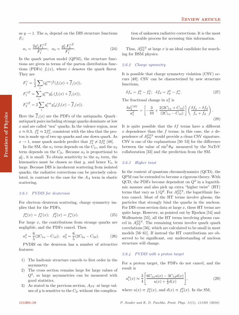
2.6.1 PVDIS for deuterium

For electron–deuteron scattering, charge symmetry im-plies that for the PDFs,

fpu(x) = fn

d (x); fpd (x) = fn

u (x). (25)

For large x, the contributions from strange quarks arenegligible, and the PDFs cancel. Then

ad1 =

65(2C1u − C1d); ad

3 =65(2C2u − C2d). (26)

PVDIS on the deuteron has a number of attractivefeatures:

1) The hadronic structure cancels to first order in theasymmetry.

2) The cross section remains large for large values ofQ2, so large asymmetries can be measured withgood statistics.

3) As stated in the previous section, APV at large val-ues of y is sensitive to the C2i without the complica-

tion of unknown radiative corrections. It is the mostfavorable process for accessing this information.

Thus, ADISPV at large x is an ideal candidate for search-

ing for BSM physics.

2.6.2 Charge symmetry

It is possible that charge symmetry violation (CSV) oc-curs [49]; CSV can be characterized by new structurefunctions,

δfu = fpu − fn

d ; δfd = fpd − fn

u . (27)

The fractional change in ad1 is

δaCSV1

ad1

=[− 3

10+

2(2C1u + C1d)(2C1u − C1d)

] (δfu − δfd

fu + fd

).

(28)

It is quite possible that the δf terms have a differentx dependence than the f terms; in this case, the x de-pendence of ADIS

PV would provide a clean CSV signature.CSV is one of the explanations [50–53] for the differencebetween the value of sin2 θW measured by the NuTeVcollaboration [33] and the prediction from the SM.

2.6.3 Higher twist

In the context of quantum chromodynamics (QCD), theQPM can be extended to become a rigorous theory. WithQCD, the PDFs become dependent on Q2 in a logarith-mic manner and also pick up extra “higher twist” (HT)terms that vary as 1/Q2. For ADIS

PV , the logarithmic fac-tors cancel. Most of the HT terms involve gluons, theparticles that strongly bind the quarks in the nucleon.For DIS cross section data at large x, these HT terms arequite large. However, as pointed out by Bjorken [54] andWolfenstein [55], all the HT terms involving gluons can-cel in ADIS

PV . The remaining terms involve quark–quarkcorrelations [56], which are calculated to be small in mostmodels [56–61]. If instead the HT contributions are ob-served to be significant, our understanding of nucleonstructure will change.

2.6.4 PVDIS with a proton target

For a proton target, the PDFs do not cancel, and theresult is

api (x) ≈ 3

4

[6C1uu(x) − 3C1dd(x)

u(x) + 14d(x)

], (29)

where u(x) ≡ fpu(x), and d(x) ≡ fp

d (x). In the SM,


REVIEW ARTICLE

ap1 ∼

[1 + 0.912d(x)/u(x)1 + 0.25d(x)/u(x)

]. (30)

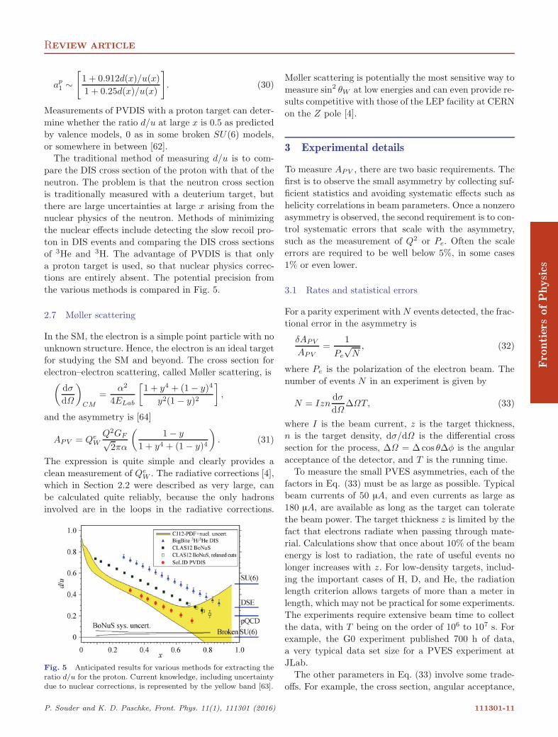
Measurements of PVDIS with a proton target can deter-mine whether the ratio d/u at large x is 0.5 as predictedby valence models, 0 as in some broken SU(6) models,or somewhere in between [62].

The traditional method of measuring d/u is to com-pare the DIS cross section of the proton with that of theneutron. The problem is that the neutron cross sectionis traditionally measured with a deuterium target, butthere are large uncertainties at large x arising from thenuclear physics of the neutron. Methods of minimizingthe nuclear effects include detecting the slow recoil pro-ton in DIS events and comparing the DIS cross sectionsof 3He and 3H. The advantage of PVDIS is that onlya proton target is used, so that nuclear physics correc-tions are entirely absent. The potential precision fromthe various methods is compared in Fig. 5.

2.7 Møller scattering

In the SM, the electron is a simple point particle with nounknown structure. Hence, the electron is an ideal targetfor studying the SM and beyond. The cross section forelectron–electron scattering, called Møller scattering, is(

dσ

dΩ

)CM

=α2

4ELab

[1 + y4 + (1 − y)4

y2(1 − y)2

],

and the asymmetry is [64]

APV = QeW

Q2GF√2πα

(1 − y

1 + y4 + (1 − y)4

). (31)

The expression is quite simple and clearly provides aclean measurement of Qe

W . The radiative corrections [4],which in Section 2.2 were described as very large, canbe calculated quite reliably, because the only hadronsinvolved are in the loops in the radiative corrections.

Fig. 5 Anticipated results for various methods for extracting theratio d/u for the proton. Current knowledge, including uncertaintydue to nuclear corrections, is represented by the yellow band [63].

Møller scattering is potentially the most sensitive way tomeasure sin2 θW at low energies and can even provide re-sults competitive with those of the LEP facility at CERNon the Z pole [4].

3 Experimental details

To measure APV , there are two basic requirements. Thefirst is to observe the small asymmetry by collecting suf-ficient statistics and avoiding systematic effects such ashelicity correlations in beam parameters. Once a nonzeroasymmetry is observed, the second requirement is to con-trol systematic errors that scale with the asymmetry,such as the measurement of Q2 or Pe. Often the scaleerrors are required to be well below 5%, in some cases1% or even lower.

3.1 Rates and statistical errors

For a parity experiment with N events detected, the frac-tional error in the asymmetry is

δAPV

APV=

1Pe

√N

, (32)

where Pe is the polarization of the electron beam. Thenumber of events N in an experiment is given by

N = Izndσ

dΩΔΩT, (33)

where I is the beam current, z is the target thickness,n is the target density, dσ/dΩ is the differential crosssection for the process, ΔΩ = Δ cos θΔφ is the angularacceptance of the detector, and T is the running time.

To measure the small PVES asymmetries, each of thefactors in Eq. (33) must be as large as possible. Typicalbeam currents of 50 µA, and even currents as large as180 µA, are available as long as the target can toleratethe beam power. The target thickness z is limited by thefact that electrons radiate when passing through mate-rial. Calculations show that once about 10% of the beamenergy is lost to radiation, the rate of useful events nolonger increases with z. For low-density targets, includ-ing the important cases of H, D, and He, the radiationlength criterion allows targets of more than a meter inlength, which may not be practical for some experiments.The experiments require extensive beam time to collectthe data, with T being on the order of 106 to 107 s. Forexample, the G0 experiment published 700 h of data,a very typical data set size for a PVES experiment atJLab.

The other parameters in Eq. (33) involve some trade-offs. For example, the cross section, angular acceptance,


REVIEW ARTICLE

and asymmetry all depend on the electron scattering an-gle θ. To keep the asymmetry reasonably constant overthe acceptance, usually Δθ/ sin θ ≡ b � 0.3.

To optimize the statistics for a parity experiment, thekinematics, including the beam energy E and scatteringangle θ, must be chosen carefully. Both the cross sectionand asymmetries depend on these parameters. For thesimplest case of elastic scattering from a heavy, spinless,isoscalar nucleus, the asymmetry and cross section aregiven by

APV = A0Q2;

dσ

dΩ=

E2 cos2(θ/2)|F |2Q4

. (34)

With this formula, we define a figure of merit (FOM),

M =dσ

dΩΔΩA2

PV ∼ Q2|F |2b cos2(θ/2)Δφ ∼ 1T

, (35)

which is proportional to the inverse of the running time.The optimum for 12C occurs for Q2 ∼ 0.02 (GeV/c)2 andis independent of the beam energy so long as the desiredQ2 occurs at forward angles. For elastic scattering fromthe proton, the form factor falls more slowly at larger Q2

values than it does for nuclei, and larger asymmetries arepossible. For DIS, the form factor is constant, and thesize of the asymmetry is limited only by the beam energy.

3.2 Accelerators

An accelerator must be available that provides a beamwith sufficient energy to obtain the desired kinemat-ics and an intensity that yields sufficient statistics. ForPVES experiments in which counting techniques areused, the duty factor is also important. These quanti-ties for various facilities are summarized in Table 3.

For PVDIS and Møller scattering, higher energies pro-vide larger asymmetries. In addition, for PVDIS, thetheoretical uncertainties are smaller at higher energies.The 11 GeV beams available with the JLab upgrade arecritical to these experiments. For elastic scattering fromnuclei, where the absolute energy resolution is criticalfor rejecting inelastic events, facilities with lower beamenergies are competitive. For elastic scattering from hy-drogen, an energy of about 3–4 GeV is ideal, but lower

Table 3 Approximate properties of accelerators used for PVESexperiments.

Accelerator facility Energy Intensity Duty factor

SLAC 20–50 GeV 10 µA 2 ×10−4

Mainz linac 300 MeV 15 µA 1.5 × 10−4

MIT-Bates 250 MeV 60 µA 10−2

JLab 1–11 GeV 100 µA CW

Mainz MAMI 0.3–1.6 GeV 30 µA CW

Mainz MESA 140 MeV 150 µA CW

energies are required for the backward angle measure-ments.

3.3 Polarized beam

A polarized beam is produced by shining circularly po-larized laser light on a semiconductor crystal. Photoelec-trons are accelerated in a static electric field and injectedinto the accelerator. The helicity of the laser light can bereversed quickly by using an electro-optical device calleda Pockels cell. Over the years, the available polarizationand intensity have advanced considerably [65, 66]. Beamswith polarizations of over 90% and intensities of morethan 100 µA are now routinely available.

The period during which the helicity of the beam isfixed is called a window. Some experiments use pairs of“windows” with opposite helicity but randomly switchthe order of the helicity to reject noise with a constantfrequency. Other experiments use quartets with a pat-tern such as + − −+ instead of pairs. The duration ofthe window can be 1–33 ms. The pattern is synchronizedwith the frequency of the power line to reject the poten-tially largest source of noise.

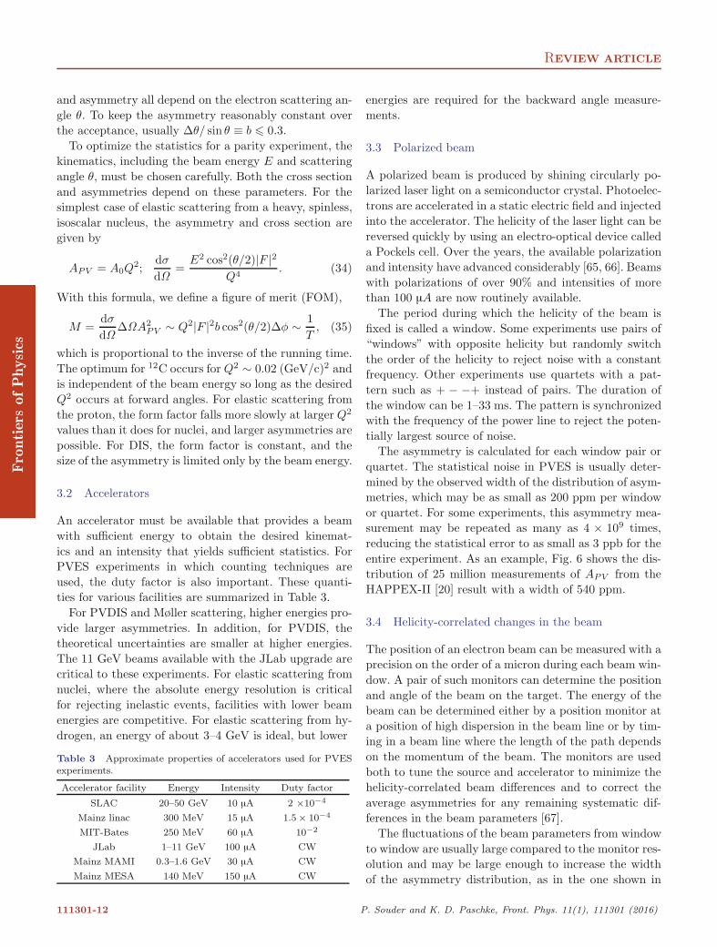
The asymmetry is calculated for each window pair orquartet. The statistical noise in PVES is usually deter-mined by the observed width of the distribution of asym-metries, which may be as small as 200 ppm per windowor quartet. For some experiments, this asymmetry mea-surement may be repeated as many as 4 × 109 times,reducing the statistical error to as small as 3 ppb for theentire experiment. As an example, Fig. 6 shows the dis-tribution of 25 million measurements of APV from theHAPPEX-II [20] result with a width of 540 ppm.

3.4 Helicity-correlated changes in the beam

The position of an electron beam can be measured with aprecision on the order of a micron during each beam win-dow. A pair of such monitors can determine the positionand angle of the beam on the target. The energy of thebeam can be determined either by a position monitor ata position of high dispersion in the beam line or by tim-ing in a beam line where the length of the path dependson the momentum of the beam. The monitors are usedboth to tune the source and accelerator to minimize thehelicity-correlated beam differences and to correct theaverage asymmetries for any remaining systematic dif-ferences in the beam parameters [67].

The fluctuations of the beam parameters from windowto window are usually large compared to the monitor res-olution and may be large enough to increase the widthof the asymmetry distribution, as in the one shown in


REVIEW ARTICLE

Fig. 6 Distribution of asymmetry measurements from theHAPPEX-II hydrogen runs.

Fig. 6. However, the monitor data may be used to correctthe asymmetries so that the width is dominated by thestatistics of the detected particles.

The dependence of the signal on the beam parame-ters can be calibrated by modulating the beam parame-ters during the run. An alternative is to use a regressionanalysis to remove correlations between the signal andthe beam parameters. Regression analysis is useful if theresolution of the measurements of the beam parametersis better than the random noise in the beam and if thebeam noise spans the beam parameter space. Becausethe modulation technique can be tuned to span the phasespace, it is generally the more reliable technique.

The systematic difference in the beam properties be-tween helicity states is most often created at the po-larized source. Here, the handedness of the circular po-larization of the laser beam determines the helicity ofthe electron beam. The Pockels cell creates this circularpolarization, with positive and negative voltage settingsselected to provide a ±λ

4 birefringence of linearly polar-ized light. The most obvious difference in the beam ariseswhen the birefringence is imperfect, such that there isa residual component of linear polarization in the laserbeam at the cathode that differs between the two polar-ization states. If this linear polarization is oriented alonga preferred axis of the photocathode quantum efficiency,the beam helicity states will differ in intensity. This effectis typically used for feedback on the helicity-correlatedbeam intensity asymmetry, where small (typically 10−2)

changes in the voltages are applied to the Pockels cell tokeep the average beam intensity asymmetry small.

Although this effect can be easily managed by mak-ing small changes to the applied voltage, note that anygradient in the birefringence of any element (includ-ing the Pockels cell or the vacuum window) will cre-ate a position-dependent asymmetry. A linear gradientacross the beam spot will evidently produce a helicity-correlated difference in the beam centroid, whereasnonzero higher moments will result in helicity-correlatedsize or shape changes in the beam spot. These positioneffects can also be created by steering or lensing in thePockels cell, as the most commonly used type (KD∗P) ispiezo-electric. These effects are controlled [68] by carefulconfiguration of the optical components to avoid intro-ducing gradients, by orienting the gradients to minimizethe sensitivity, or, when these options are exhausted, byorienting effects such that they cancel each other as muchas possible.

3.5 Slow helicity reversals

A common and very valuable technique for PVES mea-surements is to reverse the helicity of the beam in a man-ner unlike the fast reversal provided by the Pockels cell.The most common technique involves inserting, or ro-tating by 45◦, a half-wave plate (HWP) upstream of thePockels cell in the polarized source. This changes theorientation of the linearly polarized laser light by 90◦,which in turn reverses the handedness of circular polar-ized light with respect to the Pockels cell voltage. ThisHWP reversal is minimally invasive; however, if it is theonly change made, the beam helicity will change relativeto the measurement synchronization, and the measuredasymmetry will change sign.

There are two advantages to this technique. The firstis that it can be used to test the measurement. The mag-nitude of the measured asymmetry should remain thesame under the reversal. Verifying the same magnitudewith opposite sign is therefore a test that the experimentis not subject to a false asymmetry that is determined bythe Pockels cell voltage. Examples of such an asymmetrywould be a pedestal shift in the integrating detector read-out caused by the Pockels cell voltage or an uncorrectedeffect caused by piezo-electric steering in the Pockels cell.The second advantage is clear from the first: if there isan effect that changes sign with the Pockels cell, thenwhen the measured asymmetry is corrected to reflect thebeam helicity, the effect should be equal but oppositebetween the two HWP states. In this way, a slow reversalcan be used to both demonstrate the existence of a falseasymmetry and to cancel it out. The asymmetries of the


REVIEW ARTICLE

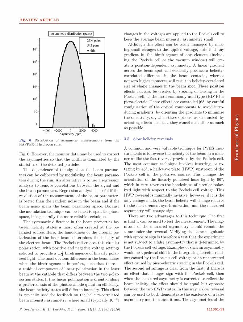
Fig. 7 The distribution of asymmetries in the HAPPEX-II hy-drogen measurement, each averaged over about 12 hours, separatedby the Half Wave Plate helicity reversal.

HAPPEX-II measurement, separated by HWP reversal,are shown in Fig. 7.

The HWP slow reversal is known to cancel helicity-correlated beam differences arising from some, but notall, causes in the polarized source. It is typically an es-sential tool for reducing the beam differences to an ac-ceptable level for an experiment. Other slow reversals arepossible. Recent experiments at JLab [29, 69] have usedspin manipulation in the low-energy injector with a com-bination of Wien rotators and solenoids to reverse thebeam helicity with minimal changes to the beam prop-erties. The E158 experiment [27] used a 6% change inbeam energy, which changed the net spin precision inthe arc entering the experimental hall and thus reversedthe beam helicity.

3.6 Targets

PVES requires thick targets that can tolerate intensebeams of 50–180 µA in order to achieve the necessarystatistics. The power deposited in the target is given by

P = ILρdE

dX, (36)

where P is the power (W), I is the current (A), L isthe target length (cm), ρ is the density (g/cm3), anddE/dX is the density of the energy deposited by an elec-tron [eV/(g/cm3)]. This corresponds, for example, to 340W for a typical 20-cm-long liquid hydrogen (LH2) targetat 20 µA.

The most common target is LH2. These targets oper-ate at a temperature near 20 K and a pressure of up to220 kPa, with a density ρ of 71 kg/m3. High-power LH2

targets with P < 1 kW were developed at SLAC in thelate 1960s, and advances were made at Caltech, includ-ing the SAMPLE [70], G0, and E158 targets. In recentyears, JLab has taken the lead in target development.

The heat has to be removed from the target to main-tain the low temperature and high density. A more subtle

problem is that the beam heat in the target can causeboiling, which introduces rapid density fluctuations thatincrease the statistical error. Rapidly reversing the he-licity of the beam addresses this problem by both re-ducing the size of the density fluctuations within a he-licity window and also increasing the statistical error ineach shorter window. Rastering the beam to a size of afew millimeters also reduces the density fluctuations. Tomaintain the desired properties of the LH2, the targetsconsist of a loop with the target cell that the beam passesthrough, a pump to maintain a high flow rate, a heat ex-changer to cool the liquid, and a heater to balance thesystem if the beam trips off.

The highest-power target built to date was used by theQweak [28] experiment. It was 35 cm long, absorbing 2.5kW in a 180 µA beam. The flow rate was on the order of 1kg/s. The density fluctuations contributed only about 50ppm at a flipping rate of 480 Hz. Recent developments incomputational fluid dynamics were critical for the designof the target.

Targets for planned experiments are even more ambi-tious. The JLab Møller target will be 150 cm long andabsorb 5 kW at 85 µA, and the 60-cm-long P2 target atMainz will absorb 4 kW at 150 µA.

Other nuclear targets, such as carbon, can easily han-dle high beam currents. A more problematic target thatis important for PVES is Pb, which has a low meltingpoint and poor thermal conductivity. For the PREx ex-periment, a diamond foil backing was used with a Pbtarget to conduct heat away from the beam spot to thefoil. When the edges were cooled to ∼20 K, it was pos-sible to operate the target at 70 µA without melting.

3.7 Spectrometers

The task of the spectrometer in a PVES experiment isto identify the desired, usually elastic, events, and alsoeliminate as much background as possible. Magnets areideal for this purpose; in a magnetic field, the deflectionof a scattered electron depends on its momentum. Neu-tral particles such as photons, which travel in straightlines, can be blocked by collimators. The position of anelectron in the detector region can be quite sensitive tothe momentum, facilitating the rejection of inelastic scat-ters, even if the energy lost is relatively small. There area number of possible configurations for magnets, manyof which have been used for PVES. Table 4 lists the spec-trometers used in past and future PVES experiments.

In this section, we will discuss the general propertiesof spectrometers. In the following subsections, we discussselected spectrometers used in PVES programs in detail.

Quadrupole magnets create a magnetic field gradient


REVIEW ARTICLE

Table 4 Apparatus for selected parity experiments. For magnets,Q=quadrupole, D=dipole.

Experiment Magnets Detector Count e− angles(◦)

SLAC E122 DQD Pb Glass No 4

Mainz None Air C No 130

MIT-Bates Q Lucite C No 35

SAMPLE None Air C No 146

HAPPEX-I QQDQ Pb-Lucite No 15

G0 Toroid Scintillator Yes 6–20; 110

A4 None PbF2 Yes 35; 145

SLAC E158 QQQQ Cu-Quartz No 2

HAPPEX-II DQQDQ Cu-Quartz No 5

PREx -I DQQDQ Quartz No 5

HAPPEX-III QQDQ Pb-Lucite No 15

PVDIS QQDQ Pb Glass Yes 19

PREx -II DQQDQ Quartz No 5

CREx DQQDQ Quartz No 4

Qweak Toroid Pb-Quartz No 5

Møller Toroid Quartz No 0.3–1

SoLID Solenoid Package Yes 22–35

P2 Solenoid Quartz No 20

Mainz C Solenoid Quartz No 40

that serves to focus charged particles, where the focallength depends on the momentum. Quadrupoles are typ-ically used in conjunction with other magnets, but somespectrometers use only quadrupoles. The 12C experimentat Bates used a pair of quadrupoles. The SLAC Møllerexperiment used a series of four quadrupoles as the spec-trometer.

The simplest magnet is the dipole, in which a rela-tively uniform field is created in a gap in an iron yoke.The iron yoke minimizes the current required to createthe field and allows flexibility in the placement of thecoils driving the field. The trajectories of the scatteredelectrons are usually perpendicular to the field lines, cre-ating the most efficient bending. Dipoles are vital forspectrometers with the highest-energy particles or themost precise resolution. The performance of dipoles isusually enhanced by using quadrupoles. The SLAC E122experiment used a spectrometer with two dipoles and aquadrupole in the middle. The high-resolution spectrom-eters (HRSs) used for the HAPPEX experiments used aspectrometer with three quadrupoles and one dipole.

Spectrometers with quadrupoles and dipoles tend tohave a small angular acceptance. For scattering at smallangles (15◦ or less), this is acceptable, as the total solidangle available at forward angles is limited. For PVESexperiments operating at larger angles, different types ofmagnets are required. Two choices are the toroid and thesolenoid. For a toroid, the field lines are in the φ direc-tion, so the field is again perpendicular to the trajecto-ries. The coils for the toroid must be in the acceptance,

so the Δφ acceptance is limited, typically to 50%. TheG0, Qweak, and proposed JLab MOLLER experimentsall use toroids. Toroidal magnets are usually designedand built especially for the experiments in which theyare used.

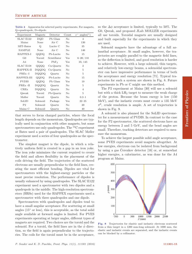
Solenoid magnets have the advantage of a full az-imuthal acceptance. At small angles, however, the tra-jectories are roughly parallel to the magnetic field lines,so the deflection is limited, and good resolution is harderto achieve. However, with a large solenoid, thin targets,and relatively low-energy beams, a solenoidal spectrom-eter can have impressive performance in terms of boththe acceptance and energy resolution [71]. Typical tra-jectories for such a system are shown in Fig. 8. Futureexperiments in Pb or C might use this method.

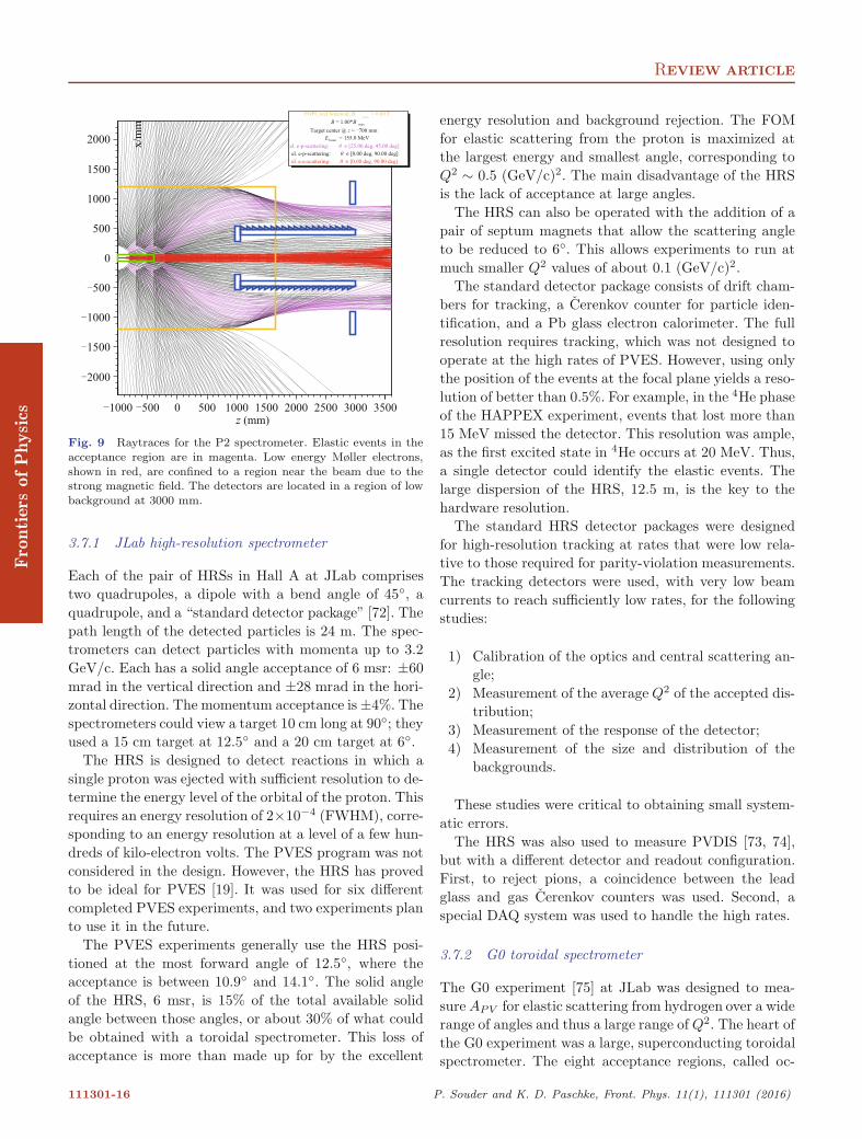
The P2 experiment at Mainz [30] will use a solenoidbut with a thick LH2 target to measure the weak chargeof the proton. Because the beam energy is low (150MeV), and the inelastic events must create a 135 MeVπ0, crude resolution is ample. A set of trajectories isshown in Fig. 9.

A solenoid is also planned for the SoLID spectrome-ter for a measurement of PVDIS. In contrast to the casefor the P2 spectrometer, the scattered electrons have anenergy between 2 and 5 GeV, and the bend angles aresmall. Therefore, tracking detectors are required to mea-sure the momentum.

To achieve the largest possible solid angle acceptance,some PVES experiments avoid magnets altogether. Atlow energies, electrons can be isolated from backgroundby using a gas Cerenkov detector [16] or, at somewhathigher energies, a calorimeter, as was done for the A4program at Mainz.

Fig. 8 Trajectories for elasitic and inelastic electrons scatteredfrom a thin target in a 1200 mm-long solenoid. At 1000 mm, theelastic and inelastic events are separated, and the inelastic eventscan be blocked by a collimator.


REVIEW ARTICLE

Fig. 9 Raytraces for the P2 spectrometer. Elastic events in theacceptance region are in magenta. Low energy Møller electrons,shown in red, are confined to a region near the beam due to thestrong magnetic field. The detectors are located in a region of lowbackground at 3000 mm.

3.7.1 JLab high-resolution spectrometer

Each of the pair of HRSs in Hall A at JLab comprisestwo quadrupoles, a dipole with a bend angle of 45◦, aquadrupole, and a “standard detector package” [72]. Thepath length of the detected particles is 24 m. The spec-trometers can detect particles with momenta up to 3.2GeV/c. Each has a solid angle acceptance of 6 msr: ±60mrad in the vertical direction and ±28 mrad in the hori-zontal direction. The momentum acceptance is ±4%. Thespectrometers could view a target 10 cm long at 90◦; theyused a 15 cm target at 12.5◦ and a 20 cm target at 6◦.

The HRS is designed to detect reactions in which asingle proton was ejected with sufficient resolution to de-termine the energy level of the orbital of the proton. Thisrequires an energy resolution of 2×10−4 (FWHM), corre-sponding to an energy resolution at a level of a few hun-dreds of kilo-electron volts. The PVES program was notconsidered in the design. However, the HRS has provedto be ideal for PVES [19]. It was used for six differentcompleted PVES experiments, and two experiments planto use it in the future.

The PVES experiments generally use the HRS posi-tioned at the most forward angle of 12.5◦, where theacceptance is between 10.9◦ and 14.1◦. The solid angleof the HRS, 6 msr, is 15% of the total available solidangle between those angles, or about 30% of what couldbe obtained with a toroidal spectrometer. This loss ofacceptance is more than made up for by the excellent

energy resolution and background rejection. The FOMfor elastic scattering from the proton is maximized atthe largest energy and smallest angle, corresponding toQ2 ∼ 0.5 (GeV/c)2. The main disadvantage of the HRSis the lack of acceptance at large angles.

The HRS can also be operated with the addition of apair of septum magnets that allow the scattering angleto be reduced to 6◦. This allows experiments to run atmuch smaller Q2 values of about 0.1 (GeV/c)2.

The standard detector package consists of drift cham-bers for tracking, a Cerenkov counter for particle iden-tification, and a Pb glass electron calorimeter. The fullresolution requires tracking, which was not designed tooperate at the high rates of PVES. However, using onlythe position of the events at the focal plane yields a reso-lution of better than 0.5%. For example, in the 4He phaseof the HAPPEX experiment, events that lost more than15 MeV missed the detector. This resolution was ample,as the first excited state in 4He occurs at 20 MeV. Thus,a single detector could identify the elastic events. Thelarge dispersion of the HRS, 12.5 m, is the key to thehardware resolution.

The standard HRS detector packages were designedfor high-resolution tracking at rates that were low rela-tive to those required for parity-violation measurements.The tracking detectors were used, with very low beamcurrents to reach sufficiently low rates, for the followingstudies:

1) Calibration of the optics and central scattering an-gle;

2) Measurement of the average Q2 of the accepted dis-tribution;

3) Measurement of the response of the detector;4) Measurement of the size and distribution of the

backgrounds.

These studies were critical to obtaining small system-atic errors.

The HRS was also used to measure PVDIS [73, 74],but with a different detector and readout configuration.First, to reject pions, a coincidence between the leadglass and gas Cerenkov counters was used. Second, aspecial DAQ system was used to handle the high rates.

3.7.2 G0 toroidal spectrometer

The G0 experiment [75] at JLab was designed to mea-sure APV for elastic scattering from hydrogen over a widerange of angles and thus a large range of Q2. The heart ofthe G0 experiment was a large, superconducting toroidalspectrometer. The eight acceptance regions, called oc-


REVIEW ARTICLE

tants, were between the eight coils comprising the toroid.The configuration allowed a total Δφ acceptance of 41%of the full azimuth. The experiment was conducted intwo phases. The first phase measured APV for electronsscattered in the forward direction at a beam energy of3.03 GeV, and the second made measurements at back-ward angles with beam energies of 0.359 and 0.684 GeV.

In contrast to most PVES experiments, which detectthe scattered electron, the first phase of G0 detected therecoil proton in the range 52◦ < θp < 77◦, correspondingto electrons scattered between 6◦ and 21◦. The electronswere not detected. The protons for each octant were de-tected by a set of 15 scintillators, with a total of 120 de-tectors in all. In typical operation, the continuous-wave(CW) JLab accelerator delivers beam bunches to eachexperimental hall with a spacing of 2 ns. For the G0experiment, the source laser was pulsed at a lower fre-quency, so that only one in 16 cycles was generated at thesource, and the beam bunches were separated by 32 ns.Consequently, the time of flight could be used to separatethe slower protons from pions and other backgrounds.

Using 700 h of data in the forward-angle configura-tion, the G0 collaboration published asymmetries for 18bins in Q2 covering the range 0.122–0.997 (GeV/c)2. Forthe lower Q2 points, the bins corresponded to individ-ual scintillators. The three highest Q2 bins came fromone scintillator and were separated using time-of-flightdata. Over that range, the asymmetry varied by almost2 orders of magnitude, from about 1 to 40 ppm. Theasymmetries included some of the smallest measured inparity-violating electron–proton scattering to that date.

Even though some of the asymmetries were small andprecisely measured, the uncertainties due to helicity-correlated beam changes (see Section 3.4) were at theimpressively small level of 0.01 ppm and entirely negli-gible. However, there were a number of more importantsystematic errors that were unique to the G0 apparatus.At the high-rate and low-asymmetry points, the rates inthe scintillators were on the order of 2 MHz, resultingin 10%–15% dead time corrections that produced uncer-tainties on the order of 0.05 ppm. About 0.1% of thebeam was in the nominally unoccupied beam bunches.These out-of-time electrons were detected in the beamintensity monitor, but the corresponding out-of-time sig-nal protons were not included in the time-of-flight cut.The correction for this effect was surprisingly large, 0.71± 0.14 ppm. For the higher-Q2 points, the uncertaintiesin the backgrounds were more important. One problemwas that the very small backgrounds from decays of po-larized hyperons produced in the target had very largeasymmetries due to the large parity violation in theirdecays.

For the second phase of the experiment, the setupwas significantly reconfigured to measure APV at back-ward scattering angles. The spectrometer was turnedaround and configured so that backward-scattered elec-trons would be detected on the scintillator bars. An ad-ditional set of scintillators located near the target wereused in coincidence to define the kinematic bins. An aero-gel Cerenkov detector was used in anticoincidence to re-ject pions.

In contrast to the situation for small angles, whereAPV varies rapidly with the kinematics, the asymmetryis fairly flat at backward angles, and only one Q2 pointwas obtained at each of the two beam energies studied.Both hydrogen and deuterium targets were used to helpreduce the uncertainties from radiative corrections (seeSection 2.4). Two Q2 points were measured, 0.221 and0.628 (GeV/c)2. For the low-Q2 point at back angles,the dominant term in the asymmetry (the AM term; seeSection 2.4) is not suppressed by 1 − 4 sin2 θW , so theasymmetries are much larger than for the forward data.One of the most important systematic uncertainties arosefrom dead time corrections, especially for the deuteriumdata, where the background rates from pions were thehighest.

3.7.3 Crystal spectrometer at Mainz

At Mainz, a spectrometer that was developed for PVESachieved a large solid angle by dispensing entirely witha magnet. The idea was to use an array of 1022 PbF2

crystals [76, 77] at a distance of 0.5 m from the target toaccept events scattered from 30◦ to 40◦, achieving a totalsolid angle of 0.6 sr. The crystals rely only on Cerenkovlight, so they are very fast and are insensitive to slowbackground particles. Given the CW beam and the largenumber of channels, the event rate of 5 × 107/s wasmanageable. An elaborate system of electronics sums allcombinations of nine adjacent crystals and produces his-tograms of the energy spectra. Because the beam energyis 854 or 570 MeV, the 3.9%/

√E resolution is sufficient

to reject inelastic events, which must be more than 100MeV below the elastic peak. The dominant backgroundwas due to quasi-elastic scattering from the aluminumtarget windows. There was also less than 1% backgrounddue to photons from π0 decay.

The apparatus could also be rotated 180◦ about a ver-tical axis through the target to subtend back angles be-tween 140◦ and 150◦. In this configuration, a layer ofplastic scintillator was added in front of the PbF2 crys-tals, allowing the separation of electrons from the pho-tons from π0 decay. The asymmetry of the remainingphoton background was determined by measuring the


REVIEW ARTICLE

asymmetry of the non-coincidence events between theplastic and crystal scintillators. Conversion of photonsinto e+e− pairs formed a significant background, whichwas corrected for using a Monte Carlo simulation. Mea-surements of APV from the proton were made using thisapparatus in the forward angle at Q2 points of 0.108 and0.23 (GeV/c)2 and in the backward angle at Q2 = 0.22(GeV/c)2 [24–26].3.7.4 The Qweak spectrometer

The Qweak spectrometer was designed to measure APV

for hydrogen at a sufficiently low Q2 that QW (p) couldbe measured. The heart of the Qweak spectrometer wasan eight-coil toroid about 3 m long. In contrast to thoseof the G0 toroid, the coils for Qweak were resistive. Thetoroid had a maximum field of 0.5 T and an

∫B · dl of

0.89 T-m. It focused electrons from a LH2 target 6.5 mupstream onto quartz bars 5.7 m downstream. The elec-trons were bent away from the beam. Inelastic events hadlarger bending angles and missed the detectors. The ac-ceptance was defined by a set of three collimators, whichgave a scattering angle of 7.9◦ ± 3◦ and an azimuthalacceptance of 49% of 2π.

The detectors were 100 cm long by 18 cm wide by 1.25cm thick and oriented in an octagon. Each detector hadan event rate of 640 MHz. The detectors were locatedin a heavily shielded cave to minimize backgrounds. Aset of drift chambers could be inserted into the spec-trometer for special data runs with very low intensity tostudy the detector response, spectrometer acceptance,and backgrounds. Results of those studies were used tobenchmark the simulation that was used to determinethe Q2 value of the APV measurement.

3.7.5 JLab SoLID spectrometer

The SoLID collaboration has designed a solenoidal spec-trometer to implement three physics programs:

1) PVDIS with deuterium, proton, and nuclear targets[78];

2) Semi-inclusive DIS (SIDIS) with polarized targets,especially 3He, where a pion is also detected in thefinal state;

3) Measurement of the cross section for the productionof the J/Ψ particle near threshold.

This proposed facility is unique at JLab in that it canoperate with both large acceptance and high luminosity.

The SoLID spectrometer uses a 1.5 T superconductingsolenoid 3.5 m long and 2.9 m in diameter. The magnetwas formerly used in the CLEO facility at Cornell.

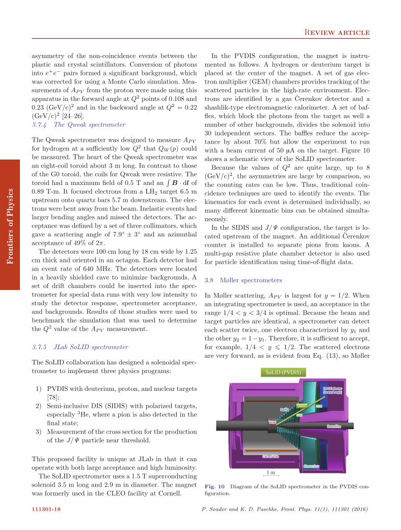
In the PVDIS configuration, the magnet is instru-mented as follows. A hydrogen or deuterium target isplaced at the center of the magnet. A set of gas elec-tron multiplier (GEM) chambers provides tracking of thescattered particles in the high-rate environment. Elec-trons are identified by a gas Cerenkov detector and ashashlik-type electromagnetic calorimeter. A set of baf-fles, which block the photons from the target as well anumber of other backgrounds, divides the solenoid into30 independent sectors. The baffles reduce the accep-tance by about 70% but allow the experiment to runwith a beam current of 50 µA on the target. Figure 10shows a schematic view of the SoLID spectrometer.

Because the values of Q2 are quite large, up to 8(GeV/c)2, the asymmetries are large by comparison, sothe counting rates can be low. Thus, traditional coin-cidence techniques are used to identify the events. Thekinematics for each event is determined individually, somany different kinematic bins can be obtained simulta-neously.

In the SIDIS and J/Ψ configuration, the target is lo-cated upstream of the magnet. An additional Cerenkovcounter is installed to separate pions from kaons. Amulti-gap resistive plate chamber detector is also usedfor particle identification using time-of-flight data.

3.8 Møller spectrometers

In Møller scattering, APV is largest for y = 1/2. Whenan integrating spectrometer is used, an acceptance in therange 1/4 < y < 3/4 is optimal. Because the beam andtarget particles are identical, a spectrometer can detecteach scatter twice, one electron characterized by y1 andthe other y2 = 1−y1. Therefore, it is sufficient to accept,for example, 1/4 < y � 1/2. The scattered electronsare very forward, as is evident from Eq. (13), so Møller

Fig. 10 Diagram of the SoLID spectrometer in the PVDIS con-figuration.


REVIEW ARTICLE

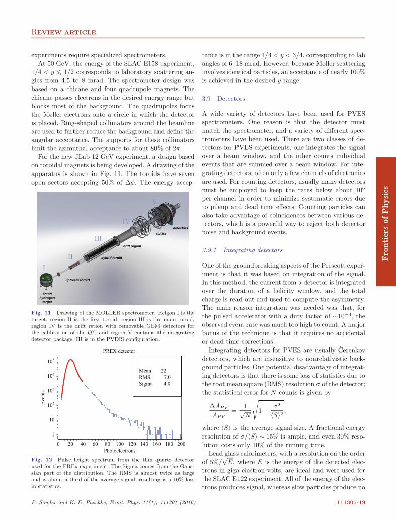
experiments require specialized spectrometers.At 50 GeV, the energy of the SLAC E158 experiment,

1/4 < y � 1/2 corresponds to laboratory scattering an-gles from 4.5 to 8 mrad. The spectrometer design wasbased on a chicane and four quadrupole magnets. Thechicane passes electrons in the desired energy range butblocks most of the background. The quadrupoles focusthe Møller electrons onto a circle in which the detectoris placed. Ring-shaped collimators around the beamlineare used to further reduce the background and define theangular acceptance. The supports for these collimatorslimit the azimuthal acceptance to about 80% of 2π.

For the new JLab 12 GeV experiment, a design basedon toroidal magnets is being developed. A drawing of theapparatus is shown in Fig. 11. The toroids have sevenopen sectors accepting 50% of Δφ. The energy accep-

Fig. 11 Drawing of the MOLLER spectrometer. Refgon I is thetarget, region II is the first toroid, region III is the main toroid,region IV is the drift retion with removable GEM detectors forthe calibration of the Q2, and region V contains the integratingdetector package. III is in the PVDIS configuration.

Fig. 12 Pulse height spectrum from the thin quartz detectorused for the PREx experiment. The Sigma comes from the Gaus-sian part of the distribution. The RMS is almost twice as largeand is about a third of the average signal, resulting is a 10% lossin statistics.

tance is in the range 1/4 < y < 3/4, corresponding to labangles of 6–18 mrad. However, because Møller scatteringinvolves identical particles, an acceptance of nearly 100%is achieved in the desired y range.

3.9 Detectors

A wide variety of detectors have been used for PVESspectrometers. One reason is that the detector mustmatch the spectrometer, and a variety of different spec-trometers have been used. There are two classes of de-tectors for PVES experiments; one integrates the signalover a beam window, and the other counts individualevents that are summed over a beam window. For inte-grating detectors, often only a few channels of electronicsare used. For counting detectors, usually many detectorsmust be employed to keep the rates below about 106

per channel in order to minimize systematic errors dueto pileup and dead time effects. Counting particles canalso take advantage of coincidences between various de-tectors, which is a powerful way to reject both detectornoise and background events.

3.9.1 Integrating detectors

One of the groundbreaking aspects of the Prescott exper-iment is that it was based on integration of the signal.In this method, the current from a detector is integratedover the duration of a helicity window, and the totalcharge is read out and used to compute the asymmetry.The main reason integration was needed was that, forthe pulsed accelerator with a duty factor of ∼10−4, theobserved event rate was much too high to count. A majorbonus of the technique is that it requires no accidentalor dead time corrections.

Integrating detectors for PVES are usually Cerenkovdetectors, which are insensitive to nonrelativistic back-ground particles. One potential disadvantage of integrat-ing detectors is that there is some loss of statistics due tothe root mean square (RMS) resolution σ of the detector;the statistical error for N counts is given by

ΔAPV

APV=

1√N

√1 +

σ2

〈S〉2 ,

where 〈S〉 is the average signal size. A fractional energyresolution of σ/〈S〉 ∼ 15% is ample, and even 30% reso-lution costs only 10% of the running time.

Lead glass calorimeters, with a resolution on the orderof 5%/

√E, where E is the energy of the detected elec-

trons in giga-electron volts, are ideal and were used forthe SLAC E122 experiment. All of the energy of the elec-trons produces signal, whereas slow particles produce no


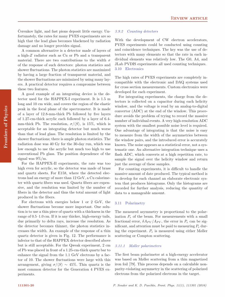
REVIEW ARTICLE

Cerenkov light, and fast pions deposit little energy. Un-fortunately, the rates for many PVES experiments are sohigh that the lead glass becomes blackened by radiationdamage and no longer provides signal.

A common alternative is a detector made of layers ofa high-Z radiator such as Cu or Pb and a transparentmaterial. There are two contributions to the width σ

of the response of such detectors: photon statistics andshower fluctuations. The photon statistics are maximizedby having a large fraction of transparent material, andthe shower fluctuations are minimized by using many lay-ers. A practical detector requires a compromise betweenthese two features.

A good example of an integrating device is the de-tector used for the HAPPEX-I experiment. It is 1.5 mlong and 10 cm wide, and covers the region of the elasticpeak in the focal plane of the spectrometer. It is madeof a layer of 12.8-mm-thick Pb followed by five layersof 1.27-cm-thick acrylic each followed by a layer of 6.4-mm-thick Pb. The resolution, σ/〈S〉, is 15%, which isacceptable for an integrating detector but much worsethan that of lead glass. The resolution is limited by theshower fluctuations; there is ample photon statistics. Theradiation dose was 40 Gy for the 30-day run, which waslow enough to use the acrylic but much too high to useconventional Pb glass. The position dependence of thesignal was 9%/m.

For the HAPPEX-II experiments, the rate was toohigh even for acrylic, so the detector was made of brassand quartz sheets. For E158, where the detected elec-trons had an energy of more than 12 GeV, a Cu calorime-ter with quartz fibers was used. Quartz fibers are expen-sive, and the resolution was limited by the number offibers in the detector and thus the total amount of lightproduced in the fibers.

For electrons with energies below 1 or 2 GeV, theshower fluctuations become more important. One solu-tion is to use a thin piece of quartz with a thickness in therange of 0.5–1.0 cm. If it is any thicker, high-energy tails,due primarily to delta rays, increase the resolution. Asthe detector becomes thinner, the photon statistics in-creases the width. An example of the response of a thinquartz detector is given in Fig. 12. The performance isinferior to that of the HAPPEX detector described abovebut is still acceptable. For the Qweak experiment, 2 cmof Pb was placed in front of a 1.25-cm-thick quartz bar toenhance the signal from the 1.1 GeV electrons by a fac-tor of 10. The shower fluctuations were large with thisarrangement, giving σ/〈S〉 ∼ 45%. Thin quartz is themost common detector for the Generation 4 PVES ex-periments.

3.9.2 Counting detectors

With the development of CW electron accelerators,PVES experiments could be conducted using countingand coincidence techniques. The key was the use of de-tectors with many elements so that the rate in each in-dividual elements was relatively low. The G0, A4, andJLab PVDIS experiments all used counting techniques.3.10 Electronics

The high rates of PVES experiments are completely in-compatible with the electronic and DAQ systems usedfor cross section measurements. Custom electronics weredeveloped for each experiment.

For integrating experiments, the charge from the de-tectors is collected on a capacitor during each helicitywindow, and the voltage is read by an analog-to-digitalconvertor (ADC) at the end of the window. This proce-dure avoids the problem of trying to record the massivenumber of individual events. A very high-resolution ADCsystem with the smallest possible noise level is required.One advantage of integrating is that the noise is easyto measure from the width of the asymmetries betweenthe window pairs, and the introduced error is accuratelyknown. The noise appears as a statistical error, not a sys-tematic one. An alternative integration technique uses aflash ADC, which converts at a high repetition rate, tosample the signal over the helicity window and returnjust the average of these samples.

For counting experiments, it is difficult to handle themassive amount of date produced. The typical method isto develop for each channel an elaborate electronic sys-tem that produces histograms. Only the histograms arerecorded for further analysis, reducing the quantity ofdata to a manageable amount.

3.11 Polarimetry

The measured asymmetry is proportional to the polar-ization Pe of the beam. For measurements with a smallfractional error, δAPV /APV , the error in Pe can be sig-nificant, and attention must be paid to measuring Pe dur-ing the experiment. Pe is measured using either Møllerscattering or Compton scattering.

3.11.1 Møller polarimeters

The first beam polarimeter at a high-energy acceleratorwas based on Møller scattering from a thin magnetizediron foil [79]. This process depends on a calculable non-parity-violating asymmetry in the scattering of polarizedelectrons from the polarized electrons in the target.


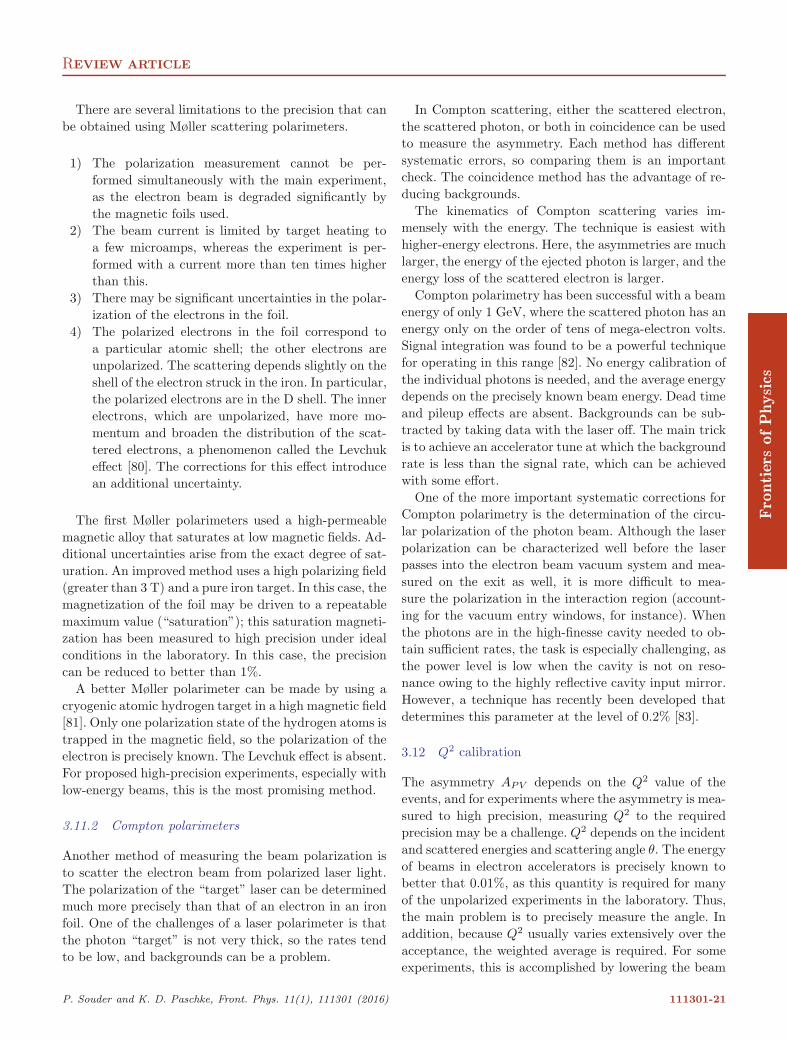
REVIEW ARTICLE

There are several limitations to the precision that canbe obtained using Møller scattering polarimeters.

1) The polarization measurement cannot be per-formed simultaneously with the main experiment,as the electron beam is degraded significantly bythe magnetic foils used.

2) The beam current is limited by target heating toa few microamps, whereas the experiment is per-formed with a current more than ten times higherthan this.

3) There may be significant uncertainties in the polar-ization of the electrons in the foil.

4) The polarized electrons in the foil correspond toa particular atomic shell; the other electrons areunpolarized. The scattering depends slightly on theshell of the electron struck in the iron. In particular,the polarized electrons are in the D shell. The innerelectrons, which are unpolarized, have more mo-mentum and broaden the distribution of the scat-tered electrons, a phenomenon called the Levchukeffect [80]. The corrections for this effect introducean additional uncertainty.

The first Møller polarimeters used a high-permeablemagnetic alloy that saturates at low magnetic fields. Ad-ditional uncertainties arise from the exact degree of sat-uration. An improved method uses a high polarizing field(greater than 3 T) and a pure iron target. In this case, themagnetization of the foil may be driven to a repeatablemaximum value (“saturation”); this saturation magneti-zation has been measured to high precision under idealconditions in the laboratory. In this case, the precisioncan be reduced to better than 1%.

A better Møller polarimeter can be made by using acryogenic atomic hydrogen target in a high magnetic field[81]. Only one polarization state of the hydrogen atoms istrapped in the magnetic field, so the polarization of theelectron is precisely known. The Levchuk effect is absent.For proposed high-precision experiments, especially withlow-energy beams, this is the most promising method.

3.11.2 Compton polarimeters

Another method of measuring the beam polarization isto scatter the electron beam from polarized laser light.The polarization of the “target” laser can be determinedmuch more precisely than that of an electron in an ironfoil. One of the challenges of a laser polarimeter is thatthe photon “target” is not very thick, so the rates tendto be low, and backgrounds can be a problem.

In Compton scattering, either the scattered electron,the scattered photon, or both in coincidence can be usedto measure the asymmetry. Each method has differentsystematic errors, so comparing them is an importantcheck. The coincidence method has the advantage of re-ducing backgrounds.

The kinematics of Compton scattering varies im-mensely with the energy. The technique is easiest withhigher-energy electrons. Here, the asymmetries are muchlarger, the energy of the ejected photon is larger, and theenergy loss of the scattered electron is larger.

Compton polarimetry has been successful with a beamenergy of only 1 GeV, where the scattered photon has anenergy only on the order of tens of mega-electron volts.Signal integration was found to be a powerful techniquefor operating in this range [82]. No energy calibration ofthe individual photons is needed, and the average energydepends on the precisely known beam energy. Dead timeand pileup effects are absent. Backgrounds can be sub-tracted by taking data with the laser off. The main trickis to achieve an accelerator tune at which the backgroundrate is less than the signal rate, which can be achievedwith some effort.

One of the more important systematic corrections forCompton polarimetry is the determination of the circu-lar polarization of the photon beam. Although the laserpolarization can be characterized well before the laserpasses into the electron beam vacuum system and mea-sured on the exit as well, it is more difficult to mea-sure the polarization in the interaction region (account-ing for the vacuum entry windows, for instance). Whenthe photons are in the high-finesse cavity needed to ob-tain sufficient rates, the task is especially challenging, asthe power level is low when the cavity is not on reso-nance owing to the highly reflective cavity input mirror.However, a technique has recently been developed thatdetermines this parameter at the level of 0.2% [83].

3.12 Q2 calibration

The asymmetry APV depends on the Q2 value of theevents, and for experiments where the asymmetry is mea-sured to high precision, measuring Q2 to the requiredprecision may be a challenge. Q2 depends on the incidentand scattered energies and scattering angle θ. The energyof beams in electron accelerators is precisely known tobetter that 0.01%, as this quantity is required for manyof the unpolarized experiments in the laboratory. Thus,the main problem is to precisely measure the angle. Inaddition, because Q2 usually varies extensively over theacceptance, the weighted average is required. For someexperiments, this is accomplished by lowering the beam


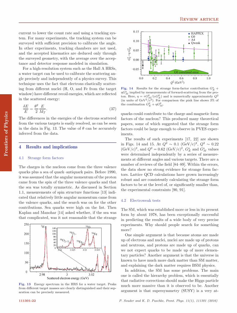
REVIEW ARTICLE

current to lower the count rate and using a tracking sys-tem. For many experiments, the tracking system can besurveyed with sufficient precision to calibrate the angle.In other experiments, tracking chambers are not used,and the accepted kinematics are deduced only throughthe surveyed geometry, with the average over the accep-tance and detector response modeled in simulation.

For a high-resolution system such as the Hall A HRSs,a water target can be used to calibrate the scattering an-gle precisely and independently of a physics survey. Thistechnique uses the fact that electrons elastically scatter-ing from different nuclei (H, O, and Fe from the targetwindow) have different recoil energies, which are reflectedin the scattered energy:

δE

E=

θ2

2E

MT. (37)

The differences in the energies of the electrons scatteredfrom the various targets is easily resolved, as can be seenin the data in Fig. 13. The value of θ can be accuratelyinferred from the data.

4 Results and implications

4.1 Strange form factors

The charges in the nucleon come from the three valencequarks plus a sea of quark–antiquark pairs. Before 1990,it was assumed that the angular momentum of the protoncame from the spin of the three valence quarks and thatthe sea was totally symmetric. As discussed in Section1.1, measurements of spin structure functions [13] indi-cated that relatively little angular momentum came fromthe valence quarks, and the search was on for the othercontributions. Sea quarks were high on the list. ThenKaplan and Manohar [14] asked whether, if the sea wasthat complicated, was it not reasonable that the strange

Fig. 13 Energy spectrum in the HRS for a water target. Peaksfrom different target masses are clearly distinguished and their sep-aration can be precisely measured.

Fig. 14 Results for the strange form-factor contribution GsE +

ηGsM implied by measurements of forward-scattering from the pro-

ton. Here, η = τGpM/(εGp

E) and is numerically approximately Q2

(in units of GeV2/c2). For comparison the pink line shows 3% ofthe combination Gp

E + ηGpM .

quarks could contribute to the charge and magnetic formfactors of the nucleon? This produced many theoreticalpapers, some of which suggested that the strange formfactors could be large enough to observe in PVES exper-iments.

The results of such experiments [17, 22] are shownin Figs. 14 and 15. At Q2 ∼ 0.1 (GeV/c)2, Q2 ∼ 0.22(GeV/c)2, and Q2 = 0.62 (GeV/c)2, Gs

E and GsM values

were determined independently by a series of measure-ments at different angles and various targets. There are anumber of reviews of the field [84–89]. Within the errors,the data show no strong evidence for strange form fac-tors. Lattice QCD calculations have grown increasinglyrobust and are consistently calculating the strange formfactors to be at the level of, or significantly smaller than,the experimental constraints [90, 91].

4.2 Electroweak tests

The SM, which was established more or less in its presentform by about 1978, has been exceptionally successfulin predicting the results of a wide body of very preciseexperiments. Why should people search for somethingmore?

One simple argument is that because atoms are madeup of electrons and nuclei, nuclei are made up of protonsand neutrons, and protons are made up of quarks, canwe not expect quarks to be made up of more elemen-tary particles? Another argument is that the universe inknown to have much more dark matter than SM matter,and explaining the dark matter requires BSM physics.

In addition, the SM has some problems. The mainone is called the hierarchy problem, which is essentiallythat radiative corrections should make the Higgs particlemuch more massive than it is observed to be. Anotherargument is that supersymmetry (SUSY) is a very at-


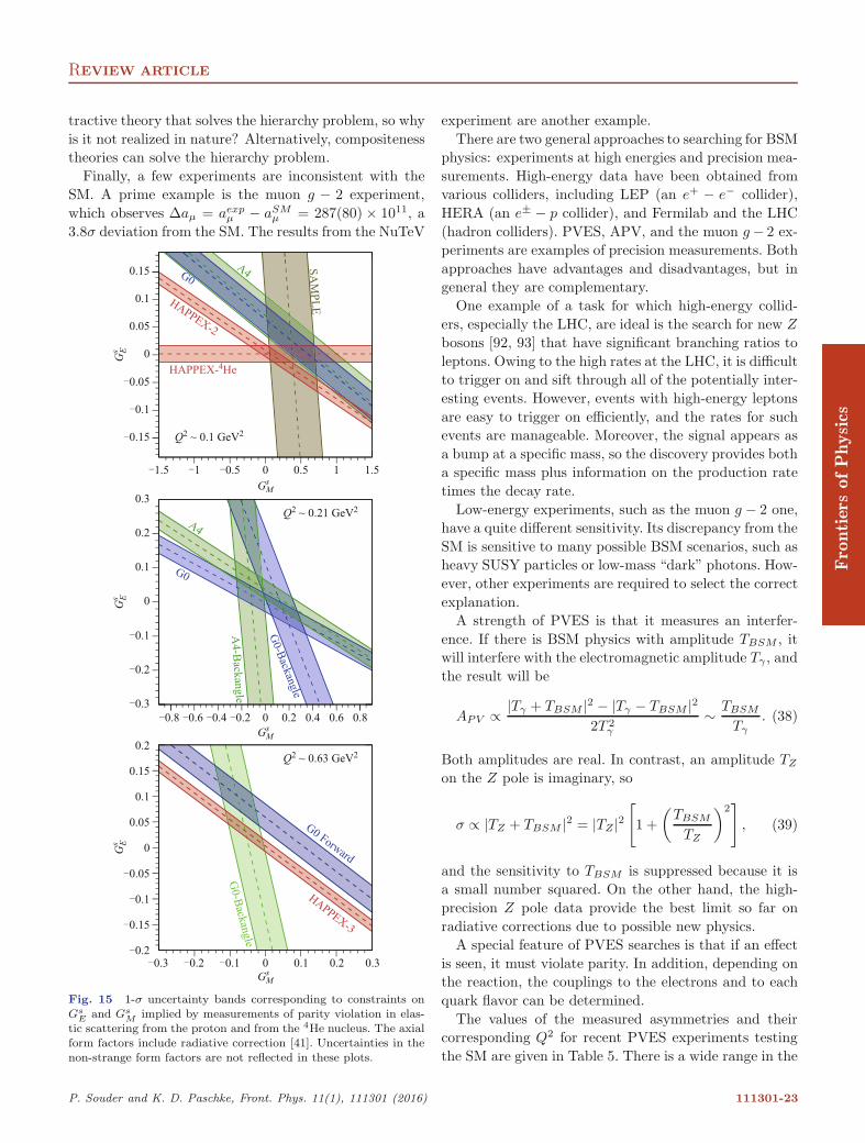
REVIEW ARTICLE

tractive theory that solves the hierarchy problem, so whyis it not realized in nature? Alternatively, compositenesstheories can solve the hierarchy problem.

Finally, a few experiments are inconsistent with theSM. A prime example is the muon g − 2 experiment,which observes Δaμ = aexp

μ − aSMμ = 287(80) × 1011, a

3.8σ deviation from the SM. The results from the NuTeV

Fig. 15 1-σ uncertainty bands corresponding to constraints onGs

E and GsM implied by measurements of parity violation in elas-

tic scattering from the proton and from the 4He nucleus. The axialform factors include radiative correction [41]. Uncertainties in thenon-strange form factors are not reflected in these plots.

experiment are another example.There are two general approaches to searching for BSM

physics: experiments at high energies and precision mea-surements. High-energy data have been obtained fromvarious colliders, including LEP (an e+ − e− collider),HERA (an e± − p collider), and Fermilab and the LHC(hadron colliders). PVES, APV, and the muon g − 2 ex-periments are examples of precision measurements. Bothapproaches have advantages and disadvantages, but ingeneral they are complementary.

One example of a task for which high-energy collid-ers, especially the LHC, are ideal is the search for new Z

bosons [92, 93] that have significant branching ratios toleptons. Owing to the high rates at the LHC, it is difficultto trigger on and sift through all of the potentially inter-esting events. However, events with high-energy leptonsare easy to trigger on efficiently, and the rates for suchevents are manageable. Moreover, the signal appears asa bump at a specific mass, so the discovery provides botha specific mass plus information on the production ratetimes the decay rate.

Low-energy experiments, such as the muon g − 2 one,have a quite different sensitivity. Its discrepancy from theSM is sensitive to many possible BSM scenarios, such asheavy SUSY particles or low-mass “dark” photons. How-ever, other experiments are required to select the correctexplanation.

A strength of PVES is that it measures an interfer-ence. If there is BSM physics with amplitude TBSM , itwill interfere with the electromagnetic amplitude Tγ , andthe result will be

APV ∝ |Tγ + TBSM |2 − |Tγ − TBSM |22T 2

γ

∼ TBSM

Tγ. (38)

Both amplitudes are real. In contrast, an amplitude TZ

on the Z pole is imaginary, so

σ ∝ |TZ + TBSM |2 = |TZ |2[1 +

(TBSM

TZ

)2]

, (39)

and the sensitivity to TBSM is suppressed because it isa small number squared. On the other hand, the high-precision Z pole data provide the best limit so far onradiative corrections due to possible new physics.

A special feature of PVES searches is that if an effectis seen, it must violate parity. In addition, depending onthe reaction, the couplings to the electrons and to eachquark flavor can be determined.

The values of the measured asymmetries and theircorresponding Q2 for recent PVES experiments testingthe SM are given in Table 5. There is a wide range in the


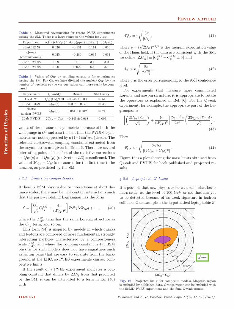
REVIEW ARTICLE

Table 5 Measured asymmetries for recent PVES experimentstesting the SM. There is a large range in the values for APV .

Experiment 〈Q2〉 (GeV/c)2 APV (ppm) σ(Stat.) σ(Syst.)

SLAC E158 0.026 –0.131 0.114 0.010

Qweak

(commisioning)0.025 –0.280 0.035 0.031

JLab PVDIS 1.09 91.1 3.1 3.0

JLab PVDIS 1.90 160.8 6.4 3.1

Table 6 Values of QW or coupling constants for experimentstesting the SM. For Cs, we have divided the nuclear QW by thenumber of nucleons so the various values can more easily be com-pared

Experiment Quantity Result SM theory

Cs APV QW (Cs)/133 −0.546 ± 0.003 0.551

SLAC E158 QW (e) 0.037 ± 0.05 0.045

elastic

nuclear PVESQW (p) 0.064 ± 0.012 0.071

JLab PVDIS 2C2u − C2d −0.145 ± 0.068 –0.095

values of the measured asymmetries because of both thewide range in Q2 and also the fact that the PVDIS asym-metries are not suppressed by a (1−4 sin2 θW ) factor. Therelevant electroweak coupling constants extracted fromthe asymmetries are given in Table 6. There are severalinteresting points. The effect of the radiative correctionson QW (e) and QW (p) (see Section 2.3) is confirmed. Thevalue of 2C2u − C2d is measured for the first time to benonzero, as predicted by the SM.

4.2.1 Limits on compositeness

If there is BSM physics due to interactions at short dis-tance scales, there may be new contact interactions suchthat the parity-violating Lagrangian has the form

L =[GF√

2CSM

1q +4π

(ΛeqAV )2

]eγμγ5eqγμq + . . . , (40)

where the ΛeqAV term has the same Lorentz structure as

the C1q term, and so on.This form [94] is inspired by models in which quarks

and leptons are composed of more fundamental, stronglyinteracting particles characterized by a compositenessscale Λeq

AV and where the coupling constant is 4π. BSMphysics for such models does not have signatures suchas lepton pairs that are easy to separate from the back-ground at the LHC, so PVES experiments can set com-petitive limits.

If the result of a PVES experiment indicates a cou-pling constant that differs by ΔCij from that predictedby the SM, it can be attributed to a term in Eq. (40)with

ΛeqAV = v

√8π

|Cij | , (41)

where v = (√

2GF )−1/2 is the vacuum expectation valueof the Higgs field. If the data are consistent with the SM,we define |ΔC±

ij | ≡ |Cexpij − CSM

ij ± σ| and

Λ± > v

√8π

|ΔC±ij |

, (42)

where σ is the error corresponding to the 95% confidencelevel.

For experiments that measure more complicatedLorentz and isospin structure, it is appropriate to rotatethe operators as explained in Ref. [6]. For the Qweakexperiment, for example, the appropriate part of the La-grangian is[(

2C1u+C1d√5

)+

4π

(ΛpAV )2

]eγμγ5e

2v2

(2uγμu+eγμd√

5

).

(43)

Then

ΛpAV > v

√8√

5π|(2C2u + C2d)±| . (44)

Figure 16 is a plot showing the mass limits obtained fromQweak and PVDIS for both published and projected re-sults.

4.2.2 Leptophobic Z′ boson

It is possible that new physics exists at a somewhat lowermass scale, at the level of 100 GeV or so, that has yetto be detected because of its weak signature in hadroncolliders. One example is the hypothetical leptophobic Z ′

Fig. 16 Projected limits for composite models. Magenta regionis excluded by published data. Orange region can be excluded withthe SoLID PVES experiment and the final Qweak results.


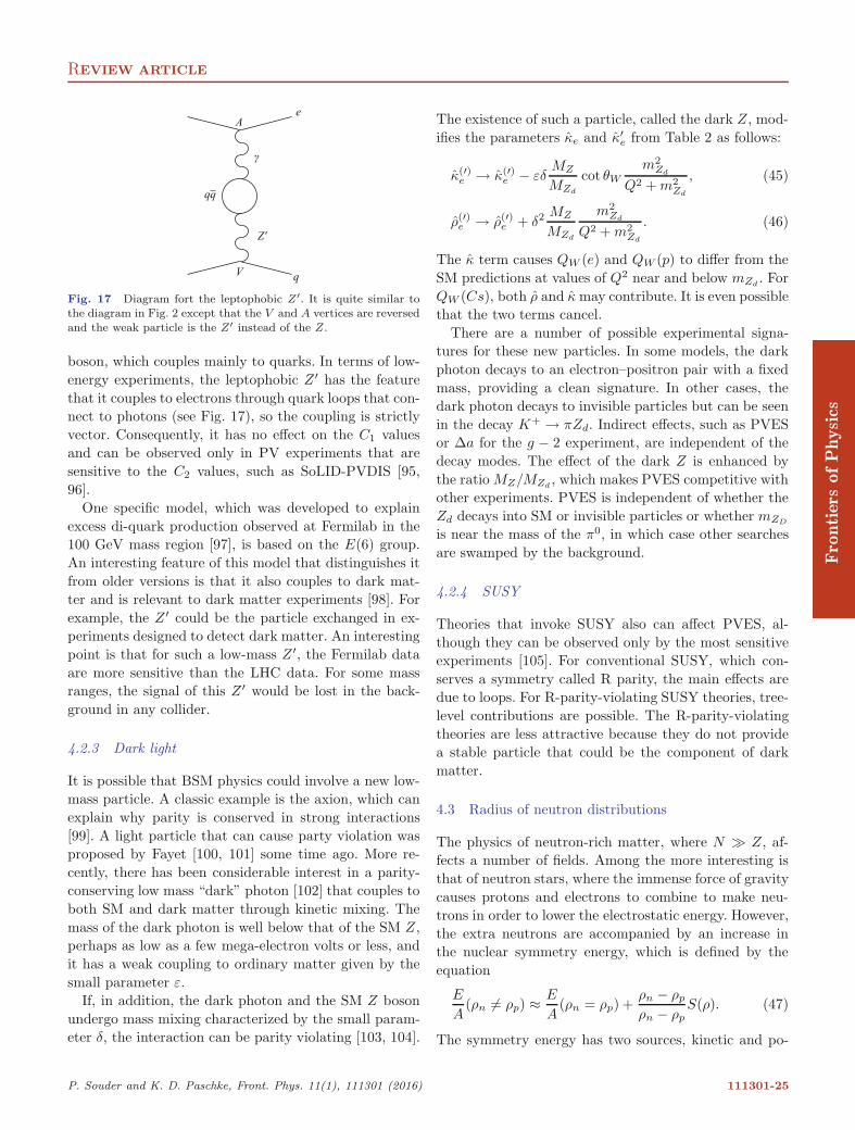
REVIEW ARTICLE

Fig. 17 Diagram fort the leptophobic Z′. It is quite similar tothe diagram in Fig. 2 except that the V and A vertices are reversedand the weak particle is the Z′ instead of the Z.

boson, which couples mainly to quarks. In terms of low-energy experiments, the leptophobic Z ′ has the featurethat it couples to electrons through quark loops that con-nect to photons (see Fig. 17), so the coupling is strictlyvector. Consequently, it has no effect on the C1 valuesand can be observed only in PV experiments that aresensitive to the C2 values, such as SoLID-PVDIS [95,96].

One specific model, which was developed to explainexcess di-quark production observed at Fermilab in the100 GeV mass region [97], is based on the E(6) group.An interesting feature of this model that distinguishes itfrom older versions is that it also couples to dark mat-ter and is relevant to dark matter experiments [98]. Forexample, the Z ′ could be the particle exchanged in ex-periments designed to detect dark matter. An interestingpoint is that for such a low-mass Z ′, the Fermilab dataare more sensitive than the LHC data. For some massranges, the signal of this Z ′ would be lost in the back-ground in any collider.

4.2.3 Dark light

It is possible that BSM physics could involve a new low-mass particle. A classic example is the axion, which canexplain why parity is conserved in strong interactions[99]. A light particle that can cause party violation wasproposed by Fayet [100, 101] some time ago. More re-cently, there has been considerable interest in a parity-conserving low mass “dark” photon [102] that couples toboth SM and dark matter through kinetic mixing. Themass of the dark photon is well below that of the SM Z,perhaps as low as a few mega-electron volts or less, andit has a weak coupling to ordinary matter given by thesmall parameter ε.

If, in addition, the dark photon and the SM Z bosonundergo mass mixing characterized by the small param-eter δ, the interaction can be parity violating [103, 104].

The existence of such a particle, called the dark Z, mod-ifies the parameters κe and κ′

e from Table 2 as follows:

κ(′)e → κ(′)

e − εδMZ

MZd

cot θW

m2Zd

Q2 + m2Zd

, (45)

ρ(′)e → ρ(′)

e + δ2 MZ

MZd

m2Zd

Q2 + m2Zd

. (46)

The κ term causes QW (e) and QW (p) to differ from theSM predictions at values of Q2 near and below mZd

. ForQW (Cs), both ρ and κ may contribute. It is even possiblethat the two terms cancel.

There are a number of possible experimental signa-tures for these new particles. In some models, the darkphoton decays to an electron–positron pair with a fixedmass, providing a clean signature. In other cases, thedark photon decays to invisible particles but can be seenin the decay K+ → πZd. Indirect effects, such as PVESor Δa for the g − 2 experiment, are independent of thedecay modes. The effect of the dark Z is enhanced bythe ratio MZ/MZd

, which makes PVES competitive withother experiments. PVES is independent of whether theZd decays into SM or invisible particles or whether mZD

is near the mass of the π0, in which case other searchesare swamped by the background.

4.2.4 SUSY

Theories that invoke SUSY also can affect PVES, al-though they can be observed only by the most sensitiveexperiments [105]. For conventional SUSY, which con-serves a symmetry called R parity, the main effects aredue to loops. For R-parity-violating SUSY theories, tree-level contributions are possible. The R-parity-violatingtheories are less attractive because they do not providea stable particle that could be the component of darkmatter.

4.3 Radius of neutron distributions

The physics of neutron-rich matter, where N � Z, af-fects a number of fields. Among the more interesting isthat of neutron stars, where the immense force of gravitycauses protons and electrons to combine to make neu-trons in order to lower the electrostatic energy. However,the extra neutrons are accompanied by an increase inthe nuclear symmetry energy, which is defined by theequation

E

A(ρn �= ρp) ≈ E

A(ρn = ρp) +

ρn − ρp

ρn − ρpS(ρ). (47)

The symmetry energy has two sources, kinetic and po-


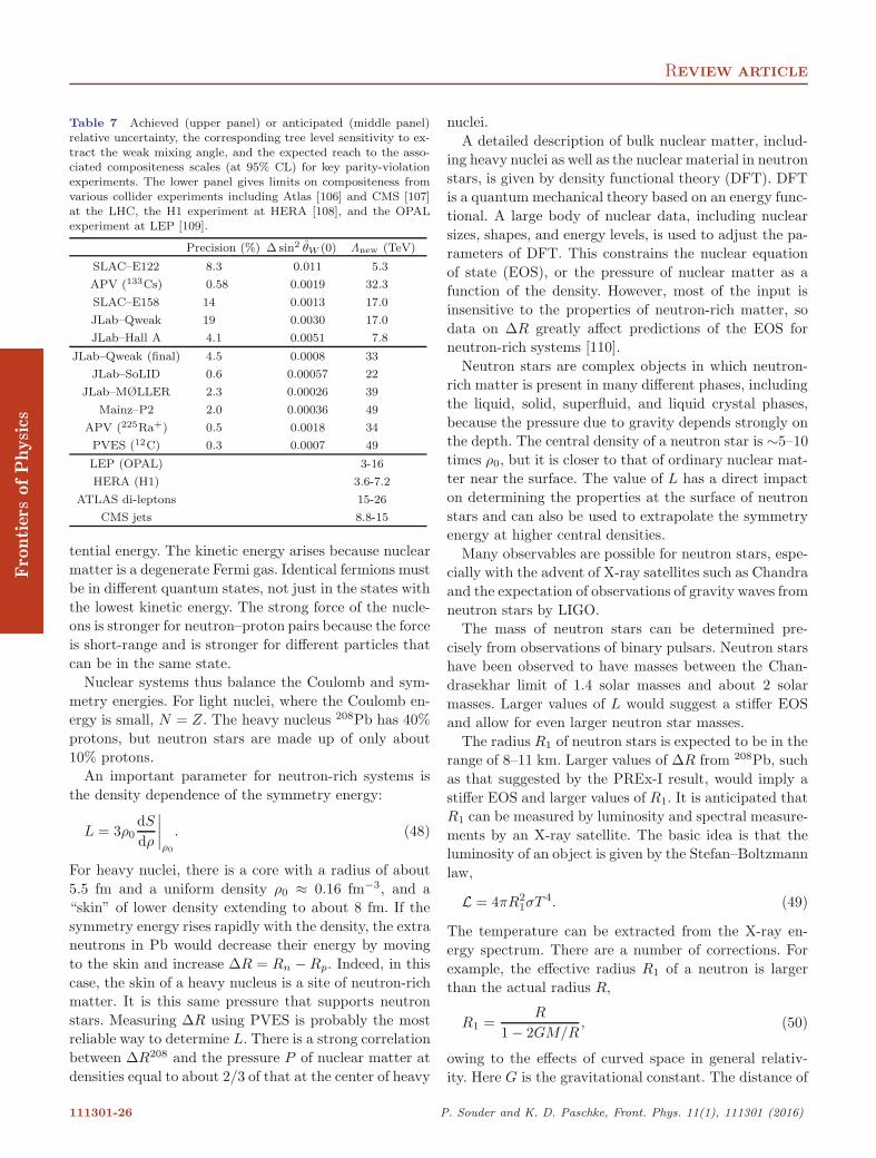
REVIEW ARTICLE

Table 7 Achieved (upper panel) or anticipated (middle panel)relative uncertainty, the corresponding tree level sensitivity to ex-tract the weak mixing angle, and the expected reach to the asso-ciated compositeness scales (at 95% CL) for key parity-violationexperiments. The lower panel gives limits on compositeness fromvarious collider experiments including Atlas [106] and CMS [107]at the LHC, the H1 experiment at HERA [108], and the OPALexperiment at LEP [109].

Precision (%) Δ sin2 θW (0) Λnew (TeV)

SLAC–E122 8.3 0.011 5.3

APV (133Cs) 0.58 0.0019 32.3

SLAC–E158 14 0.0013 17.0

JLab–Qweak 19 0.0030 17.0

JLab–Hall A 4.1 0.0051 7.8

JLab–Qweak (final) 4.5 0.0008 33

JLab–SoLID 0.6 0.00057 22

JLab–MØLLER 2.3 0.00026 39

Mainz–P2 2.0 0.00036 49

APV (225Ra+) 0.5 0.0018 34

PVES (12C) 0.3 0.0007 49

LEP (OPAL) 3-16

HERA (H1) 3.6-7.2

ATLAS di-leptons 15-26

CMS jets 8.8-15

tential energy. The kinetic energy arises because nuclearmatter is a degenerate Fermi gas. Identical fermions mustbe in different quantum states, not just in the states withthe lowest kinetic energy. The strong force of the nucle-ons is stronger for neutron–proton pairs because the forceis short-range and is stronger for different particles thatcan be in the same state.

Nuclear systems thus balance the Coulomb and sym-metry energies. For light nuclei, where the Coulomb en-ergy is small, N = Z. The heavy nucleus 208Pb has 40%protons, but neutron stars are made up of only about10% protons.

An important parameter for neutron-rich systems isthe density dependence of the symmetry energy:

L = 3ρ0dS

dρ

∣∣∣∣ρ0

. (48)

For heavy nuclei, there is a core with a radius of about5.5 fm and a uniform density ρ0 ≈ 0.16 fm−3, and a“skin” of lower density extending to about 8 fm. If thesymmetry energy rises rapidly with the density, the extraneutrons in Pb would decrease their energy by movingto the skin and increase ΔR = Rn − Rp. Indeed, in thiscase, the skin of a heavy nucleus is a site of neutron-richmatter. It is this same pressure that supports neutronstars. Measuring ΔR using PVES is probably the mostreliable way to determine L. There is a strong correlationbetween ΔR208 and the pressure P of nuclear matter atdensities equal to about 2/3 of that at the center of heavy

nuclei.A detailed description of bulk nuclear matter, includ-

ing heavy nuclei as well as the nuclear material in neutronstars, is given by density functional theory (DFT). DFTis a quantum mechanical theory based on an energy func-tional. A large body of nuclear data, including nuclearsizes, shapes, and energy levels, is used to adjust the pa-rameters of DFT. This constrains the nuclear equationof state (EOS), or the pressure of nuclear matter as afunction of the density. However, most of the input isinsensitive to the properties of neutron-rich matter, sodata on ΔR greatly affect predictions of the EOS forneutron-rich systems [110].

Neutron stars are complex objects in which neutron-rich matter is present in many different phases, includingthe liquid, solid, superfluid, and liquid crystal phases,because the pressure due to gravity depends strongly onthe depth. The central density of a neutron star is ∼5–10times ρ0, but it is closer to that of ordinary nuclear mat-ter near the surface. The value of L has a direct impacton determining the properties at the surface of neutronstars and can also be used to extrapolate the symmetryenergy at higher central densities.

Many observables are possible for neutron stars, espe-cially with the advent of X-ray satellites such as Chandraand the expectation of observations of gravity waves fromneutron stars by LIGO.

The mass of neutron stars can be determined pre-cisely from observations of binary pulsars. Neutron starshave been observed to have masses between the Chan-drasekhar limit of 1.4 solar masses and about 2 solarmasses. Larger values of L would suggest a stiffer EOSand allow for even larger neutron star masses.

The radius R1 of neutron stars is expected to be in therange of 8–11 km. Larger values of ΔR from 208Pb, suchas that suggested by the PREx-I result, would imply astiffer EOS and larger values of R1. It is anticipated thatR1 can be measured by luminosity and spectral measure-ments by an X-ray satellite. The basic idea is that theluminosity of an object is given by the Stefan–Boltzmannlaw,

L = 4πR21σT 4. (49)

The temperature can be extracted from the X-ray en-ergy spectrum. There are a number of corrections. Forexample, the effective radius R1 of a neutron is largerthan the actual radius R,

R1 =R

1 − 2GM/R, (50)

owing to the effects of curved space in general relativ-ity. Here G is the gravitational constant. The distance of


REVIEW ARTICLE

the star must be known, which is possible if it is locatedin a known globular cluster. Further, the effects of theatmosphere of the star on the X-ray spectrum must beknown.

The advanced LIGO gravitational wave observatory[111] is expected to make the first direct observationsof gravity waves in the near future [112]. Two types ofsignals arise from neutron stars:

1) Pulsar-type signals from rotating neutron stars;2) “Chirp” signals from the merging or in-spiraling of

a binary system with a neutron star.

The EOS is critical for both observations. For a rotat-ing neutron star to emit gravity waves, it must have asignificant quadrupole moment. If ΔR for 208Pb is largeenough, the solid crust of the star might be stiff enough[113] to support “mountains” of sufficient size.

The probability of observing merging neutron starsis proportional to the number of neutron stars presentin galaxies. Only hot neutron stars are directly observ-able, so the total number of neutron stars depends onhow fast they cool and thus what fraction are observed.Neutron stars cool through neutrino emission in the so-called URCA process. The rate of URCA cooling dependsstrongly on the level of the Fermi sea of the protons inthe star, which depends in turn on the symmetry energy.If the Fermi level is too high, neutrinos can be emit-ted only by a slow three-body process. The proton frac-tion in the core of the star, which determines the rate ofthe URCA cooling process, is correlated with ΔR [114].Thus, a measurement of ΔR can help predict how manysignals will be observed.

Two neutron-rich nuclei are currently of interest,208Pb, which has 44 extra neutrons, and 48Ca, whichis much lighter but still has 8 extra neutrons. The 48Canucleus is of special interest because its properties canbe computed both by DFT and also by coupled clus-ter calculations [115], which are based on nucleon forcesinstead of bulk nuclear properties. Coupled cluster cal-culations thus have the potential to provide informationon the possibility of three-neutron forces.

Isospin diffusion in heavy ion collisions, an importanttopic for exotic nuclei, depends strongly on L. The neu-tron skin also contributes to the asymmetry measured inAPV experiments. If a new generation of experiments isperformed, the PVES data will be important for makingthis correction.

The PREx experiment measured [29]

APV = 0.656± 0.060(stat) ± 0.014(syst), (51)

which implies that ΔR208 = 0.33+0.16−0.18fm. The goal of the

program is to reach a precision of 0.06 fm.

5 Summary and conclusions

Since the pioneering work of Prescott et al. in 1978, thefield of PVES has made dramatic progress. In addition toproviding a test of the SM, PVES also yields unique in-formation on the features of QCD, including strangenessin the nucleon, CSV, and the properties of HT effects.In addition, PVES probes key aspects of the propertiesof nuclear systems, including neutron stars. Over theyears, the sensitivity of experiments has improved dra-matically, as is clearly seen in Fig. 1. We are awaitingthe next generation of PVES experiments, including theP2, PREx, CREx, MOLLER, and SoLID experiments.

Acknowledgements P.A.S. is funded in part by the Departmentof Energy (DOE) under grants DE-FG02-84ER40146 (PAS) andDE-FG02-07ER41522 (KDP). We thank K. de Jager for carefullyreading the manuscript and making many helpful suggestions.

Open Access This article is distributed under the terms of theCreative Commons Attribution License which permits any use, dis-tribution, and reproduction in any medium, provided the originalauthor(s) and the source are credited.

References

1. T. Donnelly and J. Walecka, Electron scattering and nuclear

structure, Annu. Rev. Nucl. Part. Sci. 25(1), 329 (1975)

2. E. D. Bloom, D. Coward, H. DeStaebler, J. Drees, G. Miller,

L. W. Mo, R. E. Taylor, M. Breidenbach, J. I. Friedman, G.

C. Hartmann, and H. W. Kendall, High-energy inelastic e-p

scattering at 6◦ and 10◦, Phys. Rev. Lett. 23(16), 930 (1969)

3. M. Breidenbach, J. I. Friedman, H. W. Kendall, E. D.

Bloom, D. H. Coward, H. DeStaebler, J. Drees, L. W. Mo,

and R. E. Taylor, Observed behavior of highly inelastic

electron–proton scattering, Phys. Rev. Lett. 23(16), 935

(1969)

4. K. Kumar, S. Mantry, W. Marciano, and P. Souder, Low-

energy measurements of the weak mixing angle, Annu. Rev.

Nucl. Part. Sci. 63(1), 237 (2013)

5. M. J. Ramsey-Musolf, Low-energy parity-violation and new

physics, Phys. Rev. C 60(1), 015501 (1999)

6. J. Erler, C. J. Horowitz, S. Mantry, and P. A. Souder, Weak

polarized electron scattering, Annu. Rev. Nucl. Part. Sci.

64(1), 269 (2014)

7. C. S. Wu, E. Ambler, R. W. Hayward, D. D. Hoppes, and

R. P. Hudson, Experimental test of parity conservation in

beta decay, Phys. Rev. 105(4), 1413 (1957)

8. C. Y. Prescott, et al. (SLAC-E122 Collaboration), Parity

non-conservation in inelastic electron scattering, Phys. Lett.


REVIEW ARTICLE

B 77, 347 (1978)

9. C. Y. Prescott, et al. (SLAC-E122 Collaboration), Further

measurements of parity non-conservation in inelastic elec-

tron scattering, Phys. Lett. B 84, 524 (1979)

10. W. Heil, J. Ahrens, H. G. Andresen, A. Bornheimer, D. Con-

rath, K. J. Dietz, W. Gasteyer, H. J. Gessinger, W. Hart-

mann, J. Jethwa, H. J. Kluge, H. Kessler, T. Kettner, L.

Koch, F. Neugebauer, R. Neuhausen, E. W. Otten, E. Re-

ichert, F. P. Schafer, and B. Wagner, Improved limits on the

weak, neutral, hadronic axial vector coupling constants from

quasielastic scattering of polarized electrons, Nucl. Phys. B

327(1), 1 (1989)

11. P. A. Souder, R. Holmes, D. Kim, K. S. Kumar, M. E.

Schulze, K. Isakovich, G. W. Dodson, K. W. Dow, M.

Farkhondeh, S. Kowalski, M. S. Lubell, J. Bellanca, M.

Goodman, S. Patch, R. Wilson, G. D. Cates, S. Dhawan,

T. J. Gay, V. W. Hughes, A. Magnon, R. Michaels, and H.

R. Schaefer, Measurement of parity violation in the elastic

scattering of polarized electrons from 12C, Phys. Rev. Lett.

65(6), 694 (1990)

12. J. Ashman, et al. (The European Muon Collaboration), A

measurement of the spin asymmetry and determination of

the structure function g1 in deep inelastic muon-proton scat-

tering, Phys. Lett. B 206, 364 (1988)

13. J. Ashman, et al. (The European Muon Collaboration), An

investigation of the spin structure of the proton in deep in-

elastic scattering of polarised muons on polarised protons,

Nucl. Phys. B 328, 1 (1989)

14. D. B. Kaplan and A. Manohar, Strange matrix elements in

the proton from neutral-current experiments, Nucl. Phys. B

310(3–4), 527 (1988)

15. R. McKeown, Sensitivity of polarized elastic electron-proton

scattering to the anomalous baryon number magnetic mo-

ment, Phys. Lett. B 219(2–3), 140 (1989)

16. D. T. Spayde, et al. (SAMPLE Collaboration), Parity vio-

lation in elastic electron–proton scattering and the proton’s

strange magnetic form factor, Phys. Rev. Lett. 84, 1106

(2000)

17. T. Ito, et al. (SAMPLE Collaboration), Parity-violating elec-

tron deuteron scattering and the proton’s neutral weak axial

vector form factor, Phys. Rev. Lett. 92, 102003 (2004)

18. D. T. Spayde, et al. (SAMPLE Collaboration), The strange

quark contribution to the proton’s magnetic moment, Phys.

Lett. B 583, 79 (2004)

19. K. A. Aniol, et al. (HAPPEX Collaboration), Parity-

violating electroweak asymmetry in ep scattering, Phys. Rev.

C 69, 065501 (2004)

20. A. Acha, et al. (HAPPEX Collaboration), Precision mea-

surements of nucleon strange form factors at Q2 ∼ 0.1 GeV2,

Phys. Rev. Lett. 98, 032301 (2007)

21. Z. Ahmed, et al. (HAPPEX Collaboration), New precision

limit on the strange vector form factors of the proton, Phys.

Rev. Lett. 108, 102001 (2012)

22. D. S. Armstrong, et al. (G0 Collaboration), Strange-quark

contributions to parity-violating asymmetries in the forward

G0 electron-proton scattering experiment, Phys. Rev. Lett.

95, 092001 (2005)

23. D. Androic, et al. (G0 Collaboration), Strange quark con-

tributions to parity-violating asymmetries in the backward

angle G0 electron scattering experiment, Phys. Rev. Lett.

104, 012001 (2010)

24. F. Maas, et al. (A4 Collaboration), Measurement of

strange-quark contributions to the nucleon’s form factors at

Q2=0.230 (GeV/c)2 , Phys. Rev. Lett. 93, 022002 (2004)

25. F. E. Maas, K. Aulenbacher, S. Baunack, L. Capozza, J.

Diefenbach, B. Glaser, T. Hammel, D. von Harrach, Y. Imai,

E. M. Kabuss, R. Kothe, J. H. Lee, A. Lorente, E. Schilling,

D. Schwaab, M. Sikora, G. Stephan, G. Weber, C. Wein-

rich, I. Altarev, J. Arvieux, M. El-Yakoubi, R. Frascaria,

R. Kunne, M. Morlet, S. Ong, J. van de Wiele, S. Kowal-

ski, B. Plaster, R. Suleiman, and S. Taylor, Evidence for

strange-quark contributions to the nucleon’s form factors at

Q2=0.108 (GeV/c)2, Phys. Rev. Lett. 94(15), 152001 (2005)

26. S. Baunack, et al. (A4 Collaboration), Measurement of

strange quark contributions to the vector form factors of the

proton at Q2 = 0.22 (GeV/c)2, Phys. Rev. Lett. 102(15),

151803 (2009)

27. P. L. Anthony, et al. (SLAC E158 Collaboration), Precision

measurement of the weak mixing angle in Møller scattering,

Phys. Rev. Lett. 95, 081601 (2005)

28. T. Allison, et al. (Qweak Collaboration), The Qweak ex-

perimental apparatus, Nucl. Instrum. Methods A 781, 105

(2015)

29. S. Abrahamyan, et al. (PREX Collaboration), Measurement

of the neutron radius of 208Pb through parity violation in

electron scattering, Phys. Rev. Lett. 108, 112502 (2012)

30. D. Becker, et al. (P2 Collaboration), P2 - The weak charge

of the proton, PoS Bormio 2013: 024 (2013)

31. J. Benesch, et al. (MOLLER Collaboration), The MOLLER

experiment: An ultra-precise measurement of the weak mix-

ing angle using Møller scattering, arXiv: 1411.4088 [nucl-ex]

32. J. Formaggio and G. Zeller, From eV to EeV: Neutrino cross

sections across energy scales, Rev. Mod. Phys. 84(3), 1307

(2012)

33. G. P. Zeller, et al. (NuTeV Collaboration), Precise determi-

nation of electroweak parameters in neutrino-nucleon scat-

tering, Phys. Rev. Lett. 88, 091802 (2002)

34. C. S. Wood, S. C. Bennett, D. Cho, B. P. Masterson, J. L.

Roberts, C. E. Tanner, and C. E. Wieman, Measurement of

parity nonconservation and an anapole moment in cesium,

Science 275(5307), 1759 (1997)

35. G. S. Giri, O. O. Versolato, L. W. Wansbeek, J. E. van den

Berg, D. J. van der Hoek, K. Jungmann, W. L. Kruithof, C.

J. G. Onderwater, B. K. Sahoo, B. Santra, P. D. Shidling,

R. G. E. Timmermans, L. Willmann, and H. W. Wilschut,

Precision spectroscopy of trapped radioactive radium ions,

Can. J. Phys. 89(1), 69 (2011)


REVIEW ARTICLE

36. H. Frauenfelder and E. Henley, Subatomic Physics, NY:

John Wiley and Sons, 1974

37. O. Moreno, T. Donnelly, R. Gonzalez-Jimenez, and J. Ca-

ballero, Evaluation of theoretical uncertainties in parity-

violating electron scattering from nucleons and nuclei, J.

Phys. G 42(3), 034006 (2015)

38. T. Donnelly, J. Dubach, and I. Sick, Isospin dependences in

parity-violating electron scattering, Nucl. Phys. A. 503(3–

4), 589 (1989)

39. M. J. Musolf and B. R. Holstein, Electroweak corrections

to parity-violating neutral current scattering, Phys. Lett. B

242(3–4), 461 (1990)

40. A. Czarnecki and W. J. Marciano, Electroweak radiative cor-

rections to polarized Møller scattering asymmetries, Phys.

Rev. D 53(3), 1066 (1996)

41. S. L. Zhu, S. J. Puglia, B. R. Holstein, and M. J. Ramsey-

Musolf, Nucleon anapole moment and parity-violating ep

scattering, Phys. Rev. D 62(3), 033008 (2000)

42. N. Hall, P. Blunden, W. Melnitchouk, A. Thomas, and R.

Young, Hadronic γZ box corrections in Møller scattering,

Phys. Lett. B 731, 287 (2014)

43. M. Gorchtein, C. Horowitz, and M. J. Ramsey-Musolf,

Model dependence of the γZ dispersion correction to the

parity-violating asymmetry in elastic ep scattering, Phys.

Rev. C 84(1), 015502 (2011)

44. D. H. Beck, Strange-quark vector currents and parity-

violating electron scattering from the nucleon and from nu-

clei, Phys. Rev. D 39(11), 3248 (1989)

45. C. J. Horowitz, Parity violating elastic electron scattering

and Coulomb distortions, Phys. Rev. C 57(6), 3430 (1998)

46. C. J. Horowitz, S. J. Pollock, P. A. Souder, and R. Michaels,

Parity violating measurements of neutron densities, Phys.

Rev. C 63(2), 025501 (2001)

47. T. Hobbs and W. Melnitchouk, Finite-Q2 corrections to

parity-violating DIS, Phys. Rev. D 77(11), 114023 (2008)

48. G. R. Farrar and D. R. Jackson, Pion and nucleon structure

functions near x = 1, Phys. Rev. Lett. 35(21), 1416 (1975)

49. J. T. Londergan, J. C. Peng, and A. W. Thomas, Charge

symmetry at the partonic level, Rev. Mod. Phys. 82(3),

2009 (2010)

50. W. Bentz, I. C. Cloet, J. T. Londergan, and A. W. Thomas,

Reassessment of the NuTeV determination of the weak mix-

ing angle, Phys. Lett. B 693(4), 462 (2010)

51. M. Gluck, P. Jimenez-Delgado, and E. Reya, Radiatively

generated isospin violations in the nucleon and the NuTeV

anomaly, Phys. Rev. Lett. 95(2), 022002 (2005)

52. A. D. Martin, R. G. Roberts, W. J. Stirling, and R. S.

Thorne, Parton distributions incorporating QED contribu-

tions, Eur. Phys. J. C 39(2), 155 (2005)

53. C. Boros, F. M. Steffens, J. T. Londergan, and A. W.

Thomas, A new analysis of charge symmetry violation in

parton distributions, Phys. Lett. B 468(1–2), 161 (1999)

54. J. D. Bjorken, Model-independent remarks on electron-

quark parity-violating neutral-current couplings, Phys. Rev.

D 18(9), 3239 (1978)

55. L. Wolfenstein, Testing the Weinberg–Salam model in po-

larized ed and ep deep inelastic scattering, Nucl. Phys. B

146(2), 477 (1978)

56. S. Mantry, M. J. Ramsey-Musolf, and G. F. Sacco, Exami-

nation of higher-order twist contributions in parity-violating

deep-inelastic electron-deuteron scattering, Phys. Rev. C

82(6), 065205 (2010)

57. C. Y. Seng and M. J. Ramsey-Musolf, Parity-violating deep-

inelastic electron–deuteron scattering: Higher twist and par-

ton angular momentum, Phys. Rev. C 88(1), 015202 (2013)

58. J. Qiu, Twist-4 contributions to the hadron structure func-

tions, Phys. Rev. D 42(1), 30 (1990)

59. E. Stein, M. Maul, L. Mankiewicz, and A. Schafer, Renor-

malon model predictions for power corrections to flavor-

singlet deep-inelastic structure functions, Nucl. Phys. B

536(1–2), 318 (1998)

60. A. I. Signal, Calculations of higher twist distribution func-

tions in the MIT bag model, Nucl. Phys. B 497(1–2), 415

(1997)

61. A. V. Belitsky, A. Manashov, and A. Schafer, Twist-four

corrections to parity-violating electron–deuteron scattering,

Phys. Rev. D 84(1), 014010 (2011)

62. W. Melnitchouk, I. R. Afnan, F. Bissey, and A. W. Thomas,

Comment on “Parton distributions, d/u, and higher twist

effects at high x”, Phys. Rev. Lett. 84(23), 5455 (2000)

63. J. F. Owens, A. Accardi, and W. Melnitchouk, Global parton

distributions with nuclear and finite-Q2 corrections, Phys.

Rev. D 87(9), 094012 (2013)

64. E. Derman and W. J. Marciano, Parity violating asymme-

tries in polarized electron scattering, Ann. Phys. 121(1–2),

147 (1979)

65. C. K. Sinclair, P. A. Adderley, B. M. Dunham, J. C. Han-

sknecht, P. Hartmann, M. Poelker, J. S. Price, P. M. Rutt,

W. J. Schneider, and M. Steigerwald, Development of a high

average current polarized electron source with long cath-

ode operational lifetime, Phys. Rev. ST Accel. Beams 10(2),

023501 (2007)

66. P. A. Adderley, J. Clark, J. Grames, J. Hansknecht, K.

Surles-Law, D. Machie, M. Poelker, M. L. Stutzman, and

R. Suleiman, Load-locked dc high voltage GaAs photogun

with an inverted-geometry ceramic insulator, Phys. Rev. ST

Accel. Beams 13(1), 010101 (2010)

67. K. S. Kumar and P. A. Souder, Strange quarks and parity

violation, Prog. Part. Nucl. Phys. 45, S333 (2000)

68. K. D. Paschke, Controlling helicity-correlated beam asym-

metries in a polarized electron source, Eur. Phys. J. A 32(4),

549 (2007)

69. D. Androi et al. (Qweak Collaboration), First Determination

of the Weak Charge of the Proton, Phys. Rev. Lett. 111(14),

141803 (2013)


REVIEW ARTICLE

70. E. Beise, D. Beck, E. Candell, R. Carr, F. Duncan, T. For-

est, W. Korsch, J. W. Mark, R. D. McKeown, B. A. Mueller,

M. Pitt, and S. Wells, A high power liquid hydrogen target

for parity violation experiments, Nucl. Instrum. Methods A

378(3), 383 (1996)

71. P. A. Souder and R. Holmes, New spectrometers for preci-

sion measurements of parity violation with polarized elec-

trons, Proc. Parity violation in electron scattering, World

Scientific, Pasadena, CA, Feb. 23–24, 1990, pp. 137–151

72. J. Alcornc, B. Anderson, K. Aniol, J. Annand, L. Auerbach,

et al., Basic instrumentation for Hall A at Jefferson Lab,

Nucl. Instrum. Methods A 522(3), 294 (2004)

73. D. Wang, et al. (Jefferson Lab PVDIS Collaboration), Mea-

surement of parity violation in electron-quark scattering,

Nature 506, 67 (2014)

74. D. Wang, K. Pan, R. Subedi, Z. Ahmed, K. Allada, et

al., Measurement of parity-violating asymmetry in electron-

deuteron inelastic scattering, Phys. Rev. C 91(4), 045506

(2015)

75. D. Androic, et al. (G0 Collaboration), The G0 experiment:

Apparatus for parity-violating electron scattering measure-

ments at forward and backward angles, Nucl. Instrum.

Methods A 646(1), 59 (2011)

76. P. Achenbach, S. Baunack, K. Grimm, T. Hammel, D. von-

Harrach, A. L. Ginja, F. E. Maas, E. Schilling, and H.

Stroher, Measurements and simulations of Cherenkov light

in lead fluoride crystals, Nucl. Instrum. Methods A 465(2–3),

318 (2001)

77. S. Baunack, et al. (A4 Collaboration), Real-time calibration

of the A4 electromagnetic lead fluoride (PbF2) calorimeter,

Nucl. Instrum. Methods A 640, 58 (2011)

78. P. Souder, Parity-violating DIS at JLab with 12 GeV, in:

Proceedings, 16th International Workshop on Deep Inelas-

tic Scattering and Related Subjects (DIS 2008), Conf. Proc.

C 0804071, 243 (2008)

79. P. Cooper, M. Alguard, R. Ehrlich, V. Hughes, H.

Kobayakawa, J. S. Ladish, M. S. Lubell, N. Sasao, K. P.

Schuler, P. A. Souder, G. Baum, W. Raith, K. Kondo, D.

H. Coward, R. H. Miller, C. Y. Prescott, D. J. Sherden, and

C. K. Sinclair, Polarized electron-electron scattering at GeV

energies, Phys. Rev. Lett. 34(25), 1589 (1975)

80. L. Levchuk, The intra-atomic motion of bound electrons as a

possible source of the systematic error in electron beam po-

larization measurements by means of a Møller polarimeter,

Nucl. Instrum. Methods A 345(3), 496 (1994)

81. E. Chudakov and V. Luppov, Moller polarimetry with

atomic hydrogen targets, IEEE Trans. Nucl. Sci. 51(4),

1533 (2004)

82. M. Friend, D. Parno, F. Benmokhtar, A. Camsonne, M. Dal-

ton, G. B. Franklin, V. Mamyan, R. Michaels, S. Nanda, V.

Nelyubin, K. Paschke, B. Quinn, A. Rakhman, P. Souder,

and A. Tobias, Upgraded photon calorimeter with integrat-

ing readout for the Hall A Compton polarimeter at Jefferson

Lab, Nucl. Instrum. Methods A 676, 96 (2012)

83. A. Narayan, et al., Precision electron-beam polarimetry us-

ing Compton scattering at 1 GeV, arXiv: 1509.06642 [nucl-

ex]

84. R. D. Young, J. Roche, R. D. Carlini, and A. W. Thomas,

Extracting nucleon strange and anapole form factors from

world data, Phys. Rev. Lett. 97(10), 102002 (2006)

85. J. Liu, R. D. McKeown, and M. J. Ramsey-Musolf, Global

analysis of nucleon strange form factors at low Q2, Phys.

Rev. C 76(2), 025202 (2007)

86. R. Gonzalez-Jimenez, J. A. Caballero, and T. W. Don-

nelly, Parity violation in elastic electron-nucleon scattering:

Strangeness content in the nucleon, arXiv: 1111.6918 [nucl-

th]

87. K. Paschke, A. Thomas, R. Michaels, and D. Armstrong,

Strange vector form factors from parity-violating electron

scattering, J. Phys. Conf. Ser. 299, 012003 (2011)

88. D. S. Armstrong and R. D. McKeown, Parity-violating elec-

tron scattering and the electric and magnetic strange form

factors of the nucleon, Annu. Rev. Nucl. Part. Sci. 62(1),

337 (2012)

89. R. Gonzalez-Jimenez, J. A. Caballero, and T. W. Donnelly,

Global analysis of parity-violating asymmetry data for elas-

tic electron scattering, Phys. Rev. D 90(3), 033002 (2014)

90. P. E. Shanahan, R. Horsley, Y. Nakamura, D. Pleiter, P.

E. L. Rakow, G. Schierholz, H. Stuben, A. W. Thomas, R.

D. Young, and J. M. Zanotti, Determination of the strange

nucleon form factors, Phys. Rev. Lett. 114(9), 091802 (2015)

91. J. Green, S. Meinel, and M. Engelhardt, S. Krieg, J.

Laeuchli, J. Negele, K. Orginos, A. Pochinsky, and S.

Syritsyn, High-precision calculation of the strange nucleon

electromagnetic form factors, Phys. Rev. D 92(3), 031501

(2015), arXiv: 1505.01803 [hep-lat]

92. P. Langacker, The physics of heavy Z′ gauge bosons, Rev.

Mod. Phys. 81(3), 1199 (2009)

93. T. G. Rizzo, Z′ phenomenology and the LHC, arXiv: hep-

ph/0610104

94. E. Eichten, K. D. Lane, and M. E. Peskin, New tests for

quark and lepton substructure, Phys. Rev. Lett. 50(11), 811

(1983)

95. M. R. Buckley and M. J. Ramsey-Musolf, Precision probes

of a leptophobic Z′ boson, Phys. Lett. B 712(3), 261 (2012)

96. M. Gonzalez-Alonso and M. J. Ramsey-Musolf, Leptophobic

Z′ boson and parity-violating eD scattering, Phys. Rev. D

87(5), 055013 (2013)

97. T. Aaltonen, et al. (CDF Collaboration), Invariant mass dis-

tribution of jet pairs produced in association with a W bo-

son in pp collisions at√

s=1.96 TeV, Phys. Rev. Lett. 106,

171801 (2011)

98. M. R. Buckley, D. Hooper, and J. L. Rosner, A leptophobic

Z′ and dark matter from grand unification, Phys. Lett. B

703(3), 343 (2011)

99. J. E. Kim and G. Carosi, Axions and the strong CP problem,

Rev. Mod. Phys. 82(1), 557 (2010)


REVIEW ARTICLE

100. P. Fayet, Parity violation effects induced by a new gauge

boson, Phys. Lett. B 96(1–2), 83 (1980)

101. C. Bouchiat and P. Fayet, Constraints on the parity-

violating couplings of a new gauge boson, Phys. Lett. B

608(1–2), 87 (2005)

102. B. Holdom, Two U(1)’s and charge shifts, Phys. Lett. B

166(2), 196 (1986)

103. H. Davoudiasl, H. S. Lee, and W. J. Marciano, Dark side of

Higgs diphoton decays and muon g− 2, Phys. Rev. D 86(9),

095009 (2012)

104. H. Davoudiasl, H. S. Lee, and W. J. Marciano, “Dark” Z im-

plications for parity violation, rare meson decays, and Higgs

physics, Phys. Rev. D 85(11), 115019 (2012)

105. A. Kurylov, M. J. Ramsey-Musolf, and S. Su, Probing su-

persymmetry with parity-violating electron scattering, Phys.

Rev. D 68, 035008 (2003)

106. G. Aad, et al. (ATLAS Collaboration), Muon reconstruction

efficiency and momentum resolution of the ATLAS experi-

ment in proton–proton collisions at√

s = 7 TeV in 2010,

Eur. Phys. J. C 74, 3134 (2014)

107. V. Khachatryan, et al. (CMS Collaboration), Search for

quark contact interactions and extra spatial dimensions us-

ing dijet angular distributions in proton–proton collisions at√s = 8 TeV, Phys. Lett. B 746, 79 (2015)

108. F. D. Aaron, et al. (H1 Collaboration), Search for contact

interactions in e±p collisions at HERA, Phys. Lett. B 705,

52 (2011)

109. G. Abbiendi, et al. (OPAL Collaboration), Tests of the stan-

dard model and constraints on new physics from measure-

ments of fermion-pair production at 189–209 GeV at LEP,

Eur. Phys. J. C 33, 173 (2004)

110. S. Typel and B. A. Brown, Neutron radii and the neutron

equation of state in relativistic models, Phys. Rev. C 64,

027302 (2001)

111. J. Aasi, et al. (LIGO Scientific Collaboration and Virgo Col-

laboration), Search for gravitational waves from binary black

hole inspiral, merger, and ringdown in LIGO-Virgo data

from 2009–2010, Phys. Rev. D 87, 022002 (2013)

112. J. Aasi, et al. (LIGO Scientific), Enhanced sensitivity of the

LIGO gravitational wave detector by using squeezed states

of light, Nature Photon. 7, 613 (2013)

113. C. J. Horowitz and Kai Kadau, Breaking strain of neutron

star crust and gravitational waves, Phys. Rev. Lett. 102,

191102 (2009)

114. C. J. Horowitz and J. Piekarewicz, Constraining URCA cool-

ing of neutron stars from the neutron radius of 208Pb, Phys.

Rev. C 66, 055803 (2002)

115. G. Hagen, T. Papenbrock, M. Hjorth-Jensen, and D. J.

Dean, Coupled-cluster computations of atomic nuclei, Rept.

Prog. Phys. 77, 096302 (2014)


Documents

Parity violation in electron scattering - Home - Springer · 2.6.3 Higher twist 10 ... 4.2.4 SUSY 25 c The Author(s) 2015 ... the ﬁrst observation of parity violation in electron