Parochial interests and the centralized provision of local public goods: evidence from congressional voting on transportation projects

www.elsevier.com/locate/econbase

Journal of Public Economics 88 (2004) 845–866

Parochial interests and the centralized provision of

local public goods: evidence from congressional

voting on transportation projects$

Brian Knight

Department of Economics, Brown University, Box B, Providence, RI 02912 B, USA

Received 15 June 2002; received in revised form 14 May 2003; accepted 16 June 2003

Abstract

Local public goods financed from a national tax base provide concentrated benefits to recipient

jurisdictions but disperse costs, creating incentives for legislators to increase own-district spending

but to restrain aggregate spending due to the associated tax costs. While these common pool

incentives underpin a variety of theoretical analyses, which tend to predict inefficiencies in the

allocation of public goods, there is little direct evidence that individual legislators respond to such

incentives. To test for reactions to such incentives, this paper analyzes 1998 Congressional votes

over transportation project funding. The empirical results provide evidence that legislators respond to

common pool incentives: the probability of supporting the projects is increasing in own-district

spending and decreasing in the tax burden associated with aggregate spending. Having found that

legislators do respond to such incentives, I use the parameter estimates to calculate the efficient level

of public goods, which suggest over-spending in aggregate, especially in politically powerful

districts, and large associated deadweight loss.

D 2003 Elsevier B.V. All rights reserved.

Keywords: Local public goods; Legislative behavior; Fiscal Federation

Mississippi is getting tired of dirt roads; we want some asphalt.

Sen. Trent Lott (R, Mississippi), CQ Almanac, 1998.

The only guarantee that donor states should expect from this legislation is that they

will continue to subsidize road projects in other states.

Sen. John McCain (R, Arizona), CQ Almanac, 1998.

0047-2727/$ - see front matter D 2003 Elsevier B.V. All rights reserved.

doi:10.1016/S0047-2727(03)00064-1

$ An earlier version of this paper was titled ‘‘The Advantage and Disadvantages of Centralized Provision of

Public Goods Evidence from Congressional Voting on Transportation Projects’’.

E-mail address: [email protected] (B. Knight).

B. Knight / Journal of Public Economics 88 (2004) 845–866846

1. Introduction

In the United States, the federal government provides funding for many types of public

goods that are primarily local in nature. Examples include highways, bridges, water projects,

and airports. Such spending programs provide geographically concentrated benefits to

recipient jurisdictions but disperse costs due to a national, or common pool, tax base. In

central legislatures with locally-elected representatives, such as the US Congress, this

geographic disconnect between program benefits and costs creates incentives for legislators

to increase own-district spending because the district bears only a small share of the

associated tax costs. Countering this bias towards higher spending, each legislator has an

incentive to restrain spending in other districts due to the associated tax costs.

This characteristic of centrally-provided local public goods, concentrated benefits and

dispersed tax costs, is central to models of legislative behavior. Weingast et al. (1981)

focus on the first incentive created by common pool tax bases, namely the preference to

expand own-district spending. In their model, legislatures operate according to a

cooperative, or universalistic, norm under which each legislator independently chooses

own-district spending, leading to inefficiently high spending in every district and hence in

aggregate. In non-cooperative models of legislative bargaining, such as that of Baron and

Ferejohn (1987, 1989), both the incentives to expand own-district spending and to restrain

aggregate spending are present, and the legislative outcome is one in which public

spending is misallocated: public goods are over-provided in jurisdictions with political

power and under-provided elsewhere. The recent literature on political federalism has

applied these models of legislature behavior in order to re-address a classic question in

public economics: within a federation, which level of government should provide public

goods? By incorporating spillovers into these models of legislative behavior, this literature

has identified a trade-off between the ability of centralized governments to internalize

cross-jurisdiction spillovers and its tendency towards pork-barrel over-spending, particu-

larly in politically powerful districts.1

While the incentives created by national financing of local public goods underpin these

theoretical analyses, there is little direct evidence that legislators respond to such

incentives. In order to test for such common pool incentives, this paper uses 1998

Congressional votes over transportation project funding; this empirical voting analysis is

shown to be consistent with the two most commonly-used legislative processes in the

theoretical literature and is thus quite general. The empirical results demonstrate that

legislator choices reflect these common pool incentives: the probability of supporting

funding for the projects is increasing in own-district spending and decreasing in the tax

burden associated with aggregate spending. These results are robust to several alternative

specifications, although the tax cost relationship is statistically insignificant in several

cases. Having found that legislators do respond to such incentives, I then estimate the

underlying theoretical parameters and use these in order to calculate the degree of

inefficiency associated with the common pool problem. These calculations suggest

over-spending in aggregate, particularly in politically powerful districts, and large

associated deadweight loss.

1 See Inman and Rubinfeld (1997a,b), Besley and Coate (2003) and Lockwood (2002).

B. Knight / Journal of Public Economics 88 (2004) 845–866 847

2. Related literature

The vast majority of empirical research on common tax pool incentives has used

legislatures as the empirical unit of analysis. Inman (1988) attempts to measure the over-

provision of federal grants in the US Congress by using a 1972 shift in Congressional

norms from one of decision-making by strong political parties towards one of decentral-

ized decision-making in which each legislator internalizes only his district’s share of the

tax costs. Inman attributes a significant portion of the increase in grants after 1972 to this

shift and predicts that a decentralized Congress would have spent almost 50% less were

they forced to fully internalize tax costs, implying a deadweight loss of 17 cents for every

dollar allocated. A related literature uses variation in the size of legislatures, and hence the

degree of the common pool problem, across municipalities (Baqir, 2002), US states

(Gilligan and Matsusaka, 1995; Crain, 1999), and countries (Bradbury and Crain, 2001).

These studies have documented a positive relationship between the size of legislatures and

government spending.

Since these analyses rely on both a specification of the legislative process and maintained

behavioral assumptions on the part of legislators, analyses at the legislator level, which rely

on less stringent assumptions, are a useful complement. The only such analysis of which I

am aware is DelRossi and Inman (1999), who use variation in local cost sharing rules for

water projects to gauge the extent to which legislator demands for spending respond to the

share financed by the federal government. The estimated price elasticity of demand is large,

ranging from � 0.81 to � 2.55. Relative to DelRossi and Inman, my paper makes several

contributions. First, while DelRossi and Inman focus on the first incentive created by a

common tax pool, namely a preference to expand own-district spending due to common

pool tax bases, my analysis incorporates both this first incentive as well as a second key

incentive, a preference to restrain aggregate spending due to the associated tax liabilities.

Second, I provide a welfare analysis, which includes estimates of the efficient allocation of

public goods and the deadweight loss associated with this common pool problem. Finally,

while the analysis of DelRossi and Inman relies on exogenous policy shocks, my

methodology, which can be implemented using widely-available data on voting records

and the benefits and costs of legislation, has broader application.

This paper is also related to a broader literature on the determinants of roll-call voting

behavior in Congress. Peltzman (1985) finds that, after controlling for persistent regional

differences in ideology, Senators from states reaping the largest net benefits from federal

spending programs were more likely to support expansions of such programs, as captured

by an aggregate voting index constructed by the National Taxpayers Union. In an

examination of the electoral benefits of securing pork, Sellers (1997) finds an interesting

interaction between Congressional voting records and pork. In districts receiving substan-

tial pork, incumbents with fiscally liberal voting records perform better electorally than do

fiscal conservatives. In low-pork districts, by contrast, fiscal conservatives perform better.

Stein and Bickers (1995) note that, while many federal spending programs are concen-

trated in a minority of Congressional districts, such programs are often approved by

overwhelming majorities in Congress. They argue that, in order to guarantee passage,

special interest groups benefiting from such programs tend to make campaign contribu-

tions to a large group of representatives. Poole and Rosenthal (1997) downplay the role of


economic factors, arguing that a single dimension, which can be interpreted as ideology,

explains nearly all of variation in roll-call votes in Congress since the 1970s.

3. Theoretical framework

This theoretical section serves two purposes. First, it formally documents the common

pool incentives facing legislators to increase own-district spending but to restrain

aggregate spending. Second, the theoretical model provides a framework for measuring

legislator responses to such incentives. Given this empirical focus, the model is kept

simple, focusing on local public goods funded from a national tax base and abstracting

from other potentially important factors in the centralized provision of local public goods,

such as spillovers, heterogeneity in preferences, and economies of scale.

3.1. Setup

Consider a legislature with J (odd) members, or jurisdictions, which are indexed by j

and are of equal population N.2 The economy has J + 1 goods, a private good (c) and a

vector of local public goods [g=( g1, g2, . . ., gJ)], one for each jurisdiction. For simplicity,

individual preferences are assumed identical within and across jurisdictions. Individual

utility over the local public good and private goods is assumed quasi-linear:

Uðgj; cijÞ ¼ hðgjÞ þ cij ð1Þ

Utility from local public goods [h( gj)] is assumed increasing and concave and is

normalized such that zero utility is obtained from zero spending [h(0) = 0]. Finally, each

resident in jurisdiction j is endowed with mj units of the private good, which can be

converted into public goods at a dollar-for-dollar rate.

Given this setup, consider a normative benchmark, which will be used to evaluate the

performance of centralized governments in providing public goods. The Samuelson

provision of public projects ( gjS) can be characterized as follows:

NhVðgSj Þ ¼ 1; j ¼ 1; 2; . . . ; J ð2Þ

This expression equates the total willingness to pay across constituents to the marginal

cost of provision. While the Samuelson level of public goods would be that chosen by a

national planner, centralized legislatures consist of elected representatives, who face

incentives to serve local, rather than national, interests. The remainder of this section

documents the effects of this divergence between national and local interests on the level

and cross-jurisdiction allocation of public goods.

A key feature of centralized provision is that tax financing is assumed to be shared

equally across the federation. That is, total jurisdiction tax liabilities are given by s =G/J,

2 The equal population assumption is reasonable in this empirical analysis of Congressional districts, which

are portioned according to population.


where G is total federal public spending. This common pool feature of centralized tax

systems will play an important role below.

A legislature, consisting of one representative from each jurisdiction, chooses both the

aggregate supply of public goods (G) as well as the distribution of this budget across

jurisdictions. I abstract from agency considerations and simply assume that each

representative seeks to maximize the utility of a representative constituent:

Uðgj; g�jÞ ¼ hðgjÞ þ mj �G

NJð3Þ

I next consider two commonly-studied political processes in the theoretical literature:

legislative bargaining and universalism.

3.2. Legislative bargaining

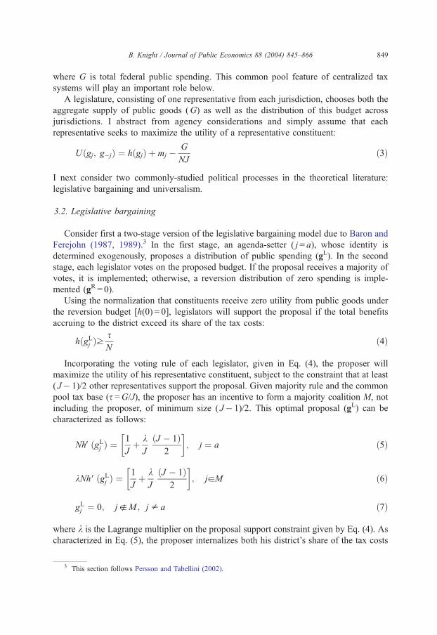
Consider first a two-stage version of the legislative bargaining model due to Baron and

Ferejohn (1987, 1989).3 In the first stage, an agenda-setter ( j= a), whose identity is

determined exogenously, proposes a distribution of public spending (gL). In the second

stage, each legislator votes on the proposed budget. If the proposal receives a majority of

votes, it is implemented; otherwise, a reversion distribution of zero spending is imple-

mented (gR = 0).

Using the normalization that constituents receive zero utility from public goods under

the reversion budget [h(0) = 0], legislators will support the proposal if the total benefits

accruing to the district exceed its share of the tax costs:

hðgLj ÞzsN

ð4Þ

Incorporating the voting rule of each legislator, given in Eq. (4), the proposer will

maximize the utility of his representative constituent, subject to the constraint that at least

( J� 1)/2 other representatives support the proposal. Given majority rule and the common

pool tax base (s =G/J), the proposer has an incentive to form a majority coalition M, not

including the proposer, of minimum size ( J� 1)/2. This optimal proposal (gL) can be

characterized as follows:

NhVðgLj Þ ¼1

Jþ k

J

ðJ � 1Þ2

� �; j ¼ a ð5Þ

kNhVðgLj Þ ¼1

Jþ k

J

ðJ � 1Þ2

� �; jaM ð6Þ

gLj ¼ 0; jgM ; j p a ð7Þ

where k is the Lagrange multiplier on the proposal support constraint given by Eq. (4). As

characterized in Eq. (5), the proposer internalizes both his district’s share of the tax costs

3 This section follows Persson and Tabellini (2002).


1/J, as well as the shadow cost k/J for each district in the size ( J� 1)/2 coalition. While

jurisdictions excluded from the coalition are under-provided, public goods are over-

provided for either the agenda-setter ( j = a), members of the winning coalition ( jaM), or

possibly both.4 Due to the incentives created by national tax financing of local public

goods, the proposer uses his agenda-setting powers in order to misallocate resources for

the benefit of his home jurisdiction and/or those jurisdictions represented in the majority

coalition. This misallocation comes at the expense of those jurisdictions excluded from the

coalition.

3.3. Universalism

Consider next the legislative model of universalism due to Weingast et al. (1981).

Given the empirical focus on voting decisions, the model is adapted to incorporate this

aspect of the political process. In the first stage, the legislature operates under a mode of

universalism; each representative independently chooses spending for their district. Taken

together, these choices on the part of representatives form a proposal (gU). In the second

stage, each representative votes over whether or not to accept this proposal, relative to a

zero reversion distribution.

Given a proposal, representatives follow voting rules identical to those of the legislative

bargaining model. That is, representatives support proposals under which the benefits

accruing to the jurisdiction exceed the tax costs associated with aggregate provision:

hðgUj ÞzsN

ð8Þ

Taking these voting rules as given, each representative chooses spending levels in order to

equate marginal jurisdictions benefits and marginal jurisdiction costs:

NhVðgUj Þ ¼1

Jð9Þ

Thus, as shown in Eq. (9), public goods are over-provided, relative to the Samuelson

condition, in every jurisdiction. Due to concentrated project benefits and dispersed tax

costs, each representative internalizes only their jurisdiction’s share of the tax costs.

4. Empirical model

This section tests for the common pool incentives documented above using the

representative voting decision rule in Eqs. (4) and (8). As demonstrated, this voting rule

is consistent with both the legislative bargaining and universalism models and thus does

not rely upon either of the assumed underlying political process. More generally, this

voting rule is consistent with any political process in which representatives, through

4 Specifically, there is no shadow cost k such that both the proposer and winning coalition members are

under-provided, relative to the Samuelson conditions. In order for both to be underprovided [NhV( gj)z 1], one

can show that 2V kV 2/J+ 1, an obvious contradiction.


majority voting, have the final authority within the legislature over proposed project

allocations.

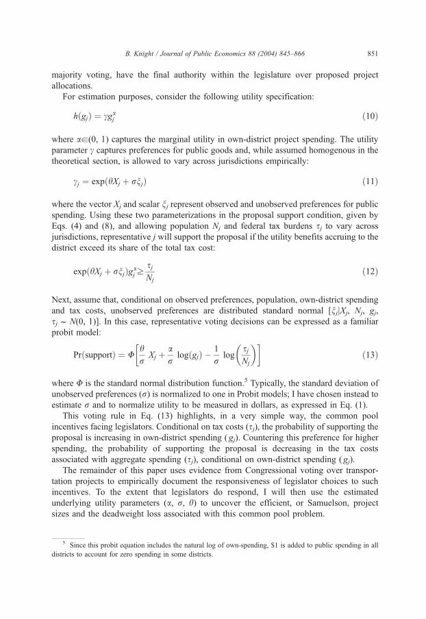
For estimation purposes, consider the following utility specification:

hðgjÞ ¼ cgaj ð10Þ

where aa(0, 1) captures the marginal utility in own-district project spending. The utility

parameter c captures preferences for public goods and, while assumed homogenous in the

theoretical section, is allowed to vary across jurisdictions empirically:

cj ¼ expðhXj þ rnjÞ ð11Þ

where the vector Xj and scalar nj represent observed and unobserved preferences for public

spending. Using these two parameterizations in the proposal support condition, given by

Eqs. (4) and (8), and allowing population Nj and federal tax burdens sj to vary across

jurisdictions, representative j will support the proposal if the utility benefits accruing to the

district exceed its share of the total tax cost:

expðhXj þ rnjÞgaj z

sjNj

ð12Þ

Next, assume that, conditional on observed preferences, population, own-district spending

and tax costs, unobserved preferences are distributed standard normal [njjXj, Nj, gj,

sjfN(0, 1)]. In this case, representative voting decisions can be expressed as a familiar

probit model:

PrðsupportÞ ¼ Uhr

Xj þar

logðgjÞ �1

rlog

sjNj

� �� ð13Þ

where U is the standard normal distribution function.5 Typically, the standard deviation of

unobserved preferences (r) is normalized to one in Probit models; I have chosen instead to

estimate r and to normalize utility to be measured in dollars, as expressed in Eq. (1).

This voting rule in Eq. (13) highlights, in a very simple way, the common pool

incentives facing legislators. Conditional on tax costs (sj), the probability of supporting theproposal is increasing in own-district spending ( gj). Countering this preference for higher

spending, the probability of supporting the proposal is decreasing in the tax costs

associated with aggregate spending (sj), conditional on own-district spending ( gj).

The remainder of this paper uses evidence from Congressional voting over transpor-

tation projects to empirically document the responsiveness of legislator choices to such

incentives. To the extent that legislators do respond, I will then use the estimated

underlying utility parameters (a, r, h) to uncover the efficient, or Samuelson, project

sizes and the deadweight loss associated with this common pool problem.

5 Since this probit equation includes the natural log of own-spending, $1 is added to public spending in all

districts to account for zero spending in some districts.


5. Transportation projects

Implementation of this empirical model requires data on legislator voting records,

district-specific public spending, and the distribution of tax liabilities across jurisdictions.

While Congressional votes on authorization or annual appropriation bills seem likely

candidates, there are several problems with this approach. First, these types of legislation

often have non-fiscal policies attached to public spending provisions.6 These provisions

tend to have differential effects across jurisdictions and thus induce both specification and

measurement error. Second, in the case of authorization or appropriation bills, the

assumption of a zero-spending reversion budget is suspect. When these bills fail to pass,

spending is typically supplemented by continuing resolutions at prior year levels, while

Congress continues the bargaining process. Thus, when deciding whether to support a

proposal, legislators trade off the provisions of the bill under consideration with both

temporary spending under continuing resolutions and future provisions likely to emerge

from ongoing negotiations. Third, federal tax incidence data across geographic entities,

such as states or congressional districts, are not readily available. The Tax Foundation

(2000) has attempted to estimate the cross-state distribution of total federal tax liabilities.

However, in doing so, one encounters thorny issues regarding economic incidence. For

example, are the burdens of the corporate income tax borne by its shareholders, customers,

or employees, each of whom may reside in different states?

To overcome these obstacles, I focus on votes over an amendment in the US House of

Representatives designed to strip away 1653 transportation projects (totaling $9.5 billion)

from the Transportation Equity Act for the 21st Century (TEA-21), which was passed in

1998 and authorized transportation spending for 1998–2003.7 This stripping amendment

failed by a 79–337 vote and the earmarked projects were included in the final

authorization bill.8 For consistency with the theoretical model, I will refer to the 337 no

votes on the stripping amendment as votes in support of the projects and the 79 yes votes

on the stripping amendment as votes in opposition of the projects. Regarding the first

problem described above, this amendment within the authorization bill had narrow

6 For example, the 1998 transportation reauthorization contained ethanol tax breaks, drunken driving

prevention incentives, air bag policies, and a ban on certain trucks.7 The amendment also stripped away $2 billion in funding for rail transit projects, although the bill did not

earmark these funds for specific projects. Rather, the bill listed projects that would be eligible to apply to the

Department of Transportation for funding. The Department would then have discretion in allocating these funds.

Due to this lack of information, I simply exclude these transit funds from the analysis.8 Given that the vote was overwhelmingly in favor of supporting the projects, votes by representatives over

this amendment may have been one of ‘‘position-taking’’. More specifically, knowing that the amendment would

fail, representatives used their votes to signal to constituents whether or not their district was a net beneficiary

from the funding of these projects. So long as these signals are accurate, however, votes over the amendment will

reflect the costs and benefits of these projects. Of course, representatives may use the vote as an opportunity to

signal the benefits and costs of not only the stripping amendment but also of the larger transportation bill.

Unfortunately, most of the funds in the larger bill were transferred to state governments, which then decided how

to allocate the resources across projects within the state. Thus, it is difficult to measure the benefits of the larger

bill across Congressional districts. In the end, this is an empirical question; to the extent that the empirical results

do not provide evidence that votes reflect the costs and benefits of these projects, one interpretation is that

representatives were sending signals to voters on the larger transportation bill.


language, restricting consideration to public spending provisions. Second, lending support

to the zero spending reversion assumption, had the amendment passed, the projects would

likely have not been included in the final legislation, since the Senate version contained no

earmarked projects and President Clinton had publicly opposed them.9 Of course, were the

amendment to pass, these projects could have been included in future legislation, such as

the transportation appropriations bill. Since such future legislation is unobserved, we view

these considerations as beyond the scope of this study and regard the zero reversion

assumption as a reasonable approximation. Regarding the third complication, measure-

ment of tax burdens at the jurisdiction level, transportation projects are funded through a

single tax, the federal gasoline tax, and the cross-state distribution of such tax liabilities is

readily available.10 While there is little formal evidence on the economic incidence of

gasoline excise taxes, Poterba (1996) and Besley and Rosen (1999) find a strong

relationship between after-tax consumer prices and sales taxes, suggesting that residents

of a jurisdiction in which commodity taxes are collected bear a substantial, if not complete,

share of the incidence.

6. Data

Summary statistics are provided in Table 1. As predicted by the theoretical model,

support for funding of these projects is increasing in own-district spending and

decreasing in tax burdens. Those districts supporting the projects tend to be smaller,

more urban and have longer commute times. Regarding industrial composition, those

supporting the projects tend to represent districts with employment in transportation and

communications and services, which is the omitted category in Table 1, although these

differences are quantitatively small. The remainder of this section describes the

construction of the two key variables in the empirical analysis: own-district spending

and tax costs.

6.1. District project spending

In order to match each of the projects with a Congressional district, I relied on the

project description in the bill. These descriptions provide a city or county name, which

could be matched with a district in the Congressional District Atlas (1998). For those cities

or counties with multiple districts, I used a variety of additional sources, including maps

from the Atlas, testimony before the Subcommittee on Surface Transportation, and press

releases from representatives’ websites. Approximately 10% of project spending could not

be assigned to a specific district, either due to the project being located in multiple districts

or insufficient information in the project description. Given this lack of information, I

9 Congressional Quarterly Almanac, 1998.10 Federal gasoline tax revenues are deposited into the Highway Trust Fund. The 1998 reauthorization

discontinued the use of this fund for general deficit reduction, effectively creating a trust fund ‘‘firewall’’, a dollar-

for-dollar correspondence between gasoline tax revenues and transportation spending.

Table 1

Summary statistics, 416 Congressional districts (sample averages, S.D. in parentheses)

Variable Support projects Not support Description Source

N= 337 N = 79

Project spending

Own spending $21 040 860 $5 743 392 Projects Author

( gj) (17 170 160) (8 306 591) in district tabulations

Coalition member 0.9169 0.4304 Positive spending Author

1 [ gj>0] (0.2764) (0.4983) in district tabulations

Tax cost $17 887 410 $18 839 510 Cost of Author prediction

(sj) ($6 198 413) ($5 170 653) proposal (see Table 2)

Demand measures

Area 0.0215 0.0299 Millions of Congressional

(0.0968) (0.0604) square kilometers districts (census)

Percent urban 0.7475 0.7291 Percent in Congressional

(0.2217) (0.2154) urban area districts (census)

Commute time 10.0588 9.7773 Average commute Congressional

(2.4523) (2.3568) (in minutes) districts (census)

Industry

Percent agriculture 0.0337 0.0423 % Employed Congressional

and mining (0.0319) (0.0358) in industry districts (Census)

Percent construction 0.24096 0.2409 % Employed Congressional

and manufacturing (0.0643) (0.0778) in industry districts (census)

Percent transportation 0.0713 0.0683 % Employed Congressional

and communication (0.0156) (0.0145) in industry districts (census)

Percent trade 0.21186 0.2171 % Employed Congressional

(0.0197) (0.0190) in industry districts (census)


simply exclude these projects from the analysis.11 Finally, since projects are funded over

the 1998–2003 horizon, spending is converted into 1998 dollars using a discount rate of

2.7%, the average rate of inflation between 1990 and 1999.

6.2. Tax costs

While the theoretical model assumed that public spending was financed exclusively

through central government tax revenues, these transportation projects were funded

through a 80% federal share and a 20% state share; each district’s share of the total tax

costs of the proposal can thus be expressed as follows:

sj ¼1

5

� �sj=s gj þ

XlaSj

gl

24

35þ 4

5

� �sj=sss=f G ð14Þ

11 As an alternative measure, I included multiple-district projects but, somewhat arbitrarily, equally allocated

the spending between the relevant districts. Results using this measure, not reported here, are similar to the

baseline results in this paper.


where sj/s is the district’s share of the state costs, ss/f is the state’s share of the federal taxes,

and Sj is the set of other districts within the state.12 Each state’s share of the federal costs

(ss/f) can be calculated using state-specific trust-fund receipts, which are available in

Highway Statistics (1998) (US Department of Transportation, 1999). Unfortunately, each

district’s share of state revenues (sj/s) are not available.

I make two attempts to resolve this data limitation. The first approach, described more

fully in the next paragraph, uses the cross-state variation in tax liabilities (ss/f) to estimate

the within-state variation (sj/s). The second approach simply aggregates the two key

district-level variables, voting decisions and project spending, from the Congressional

district-level to the state-level. After matching these measures with the state-level data on

tax liabilities, I estimate a grouped linear probability model for the sample of 50 states.

In order to estimate the within-state variation in gasoline tax receipts, I use state-level

variation in tax receipts to predict district-level receipts. More specifically, state trust fund

receipts are regressed on exogenous state characteristics, and the resulting coefficients are

then matched with exogenous district characteristics to predict receipts at the district level.

The results from this regression are provided in Table 2. Given my goal to predict

aggregate receipts at the district level, which are then converted into shares, all regressors

are measured as state aggregates.13 Only two coefficients are statistically significant, likely

reflecting the small sample of 50 states. However, the R-squared of the regression is

0.9645, suggesting strong predictive power. Using the predicted district receipts, each

district’s share of state receipts is given by:

sj=s ¼r̂eceiptsj

r̂eceiptsj þPla Sj

r̂eceiptslð15Þ

Although the within-state variation in state tax liabilities is generated from these predicted

gasoline tax receipts, it is important to note that two other sources of variation in district

gasoline tax receipts in Eq. (14), namely cross-state differences in project spending and

cross-state differences in tax liabilities, are taken from data sources and are thus independent

of the results of this prediction approach regarding variation in tax liabilities within states.

Given that users of transportation services pay a disproportionate share of gasoline

taxes, unobserved preferences for transportation services may be positively correlated with

these measured tax liabilities. To address this concern of benefits taxation, the econometric

analysis includes controls for observed preferences for transportation services, such as

area, percent urban, commute times, and the composition of employment across industries.

However, some preferences for transportation, such as geography, are difficult to measure.

While this positive correlation between unobserved preferences and gasoline tax liabilities

12 This expression implicitly assumes that state governments finance their 20% share through gasoline tax

revenues. Per Table SF-1 of US Department of Transportation (1999), Highway Statistics (1998), gasoline tax

revenues represent 52% of own-source revenues attributable to highway spending. Further, the two other largest

revenue sources, vehicle taxes (26%) and tolls (8%), should have incidence distributions that are similar to the

distribution for gasoline tax revenues since all three sources tax highway users.13 Thus, the receipts equation represents an underlying individual demand for gasoline, which has been

aggregated by summing across all state residents. Results from a per-capita specification, not reported here,

provide similar results.

Table 2

Trust fund receipts equation results, 50 states receipts source: Highway statistics, 1998 (Table FE-9) (US

Department of Transportation, 1999)

Variable Coefficient

Population 0.0731

(0.0825)

Area 3800.984

(81 005.33)

Urban � 0.0853a

(0.0514)

Commute time � 0.0052

(0.0055)

Agriculture and mining 2.3447b

(0.6365)

Construction and 0.1143

manufacturing (0.2208)

Transportation and 1.7484

communication (1.3181)

Trade 0.7066

(0.7976)

Constant � 12 301.83

(35 102.25)

R-squared 0.9645

Note: all variables measured as totals across state population.a 90% significance.b 95% significance.


may lead to biased parameter estimates, this bias with respect to the tax costs coefficient

should, if anything, be upwards and thus against measuring a negative relationship

between tax costs and support for funding of these projects.

7. Empirical results

7.1. Probit results

The results in Table 3 provide the first evidence that legislators respond to common

pool incentives to support own-district spending but to oppose tax costs associated with

aggregate spending. The first column of Table 3 presents the results of a Probit voting

model that includes only the two key independent variables from the theoretical model: log

own-district spending and log tax costs.14 As predicted by the theoretical model, the

coefficient on own-district spending is positive and statistically significant. While

14 Bootstrap standard errors, which are provided in Table 3, reflect the additional uncertainty arising from the

inclusion of log tax costs, which is a generated regressor. One hundred replications were taken from the set of

Congressional districts, and these observations were used in both the first-stage state-level tax receipts regressions

and in the second-stage Probit model. To reflect the composition of the bootstrap sample of Congressional

districts, state-level observations in the tax receipts regressions were weighted, with the weights equal to the

number of within-state Congressional districts that were represented in the bootstrap sample divided by actual

number of Congressional districts within the state.

Table 3

Representative voting decisions—baseline specification

Probit Probit FE Logit

Dependent variable Vote Vote Vote

Observations 416 416 290

Own-spending 0.1084b 0.1095b 0.1544b

(in logs) (0.0131) (0.0120) (0.0398)

Tax costs (in logs) � 0.8463b � 0.8312a � 1.9544

(0.4104) (0.4503) (2.5665)

Area � 0.4158 � 5.6771

(3.1059) (17.9221)

Percent urban 0.0229 � 0.2432

(0.7124) (2.8092)

Commute time � 0.0265 � 0.1696

(0.0734) (0.2495)

Percent agriculture � 1.1717 4.7140

and mining (4.5276) (21.7876)

Percent construction 0.9759 5.1119

and manufacturing (1.9343) (6.7321)

Percent transportation 14.5034 41.1300

and communication (9.4279) (26.1207)

Percent trade � 2.7533 5.6248

(6.3740) (19.3125)

R-squared 0.2555 0.2700 0.1836

Constant not reported, bootstrap standard errors.a 90% significance.b 95% significance.


legislators support higher own-district spending, they attempt to restrain aggregate

spending and the associated tax costs, as the coefficient on tax costs is negative and

statistically significant. These results demonstrate that legislators do act on incentives,

which are inherent in a system of local public goods financed from a national tax base, to

boost own-district spending while restraining the tax costs associated with aggregate

spending. The remainder of this paper provides evidence on the robustness of this result

and then, having found that legislators respond to common pool incentives, estimates the

efficient allocation of public goods and the deadweight loss associated with this common

pool problem.

While the theoretical model does not incorporate heterogeneity in preferences for

public goods, such heterogeneity may cast doubt on the assumption that unobserved

preferences nj are independent of spending proposals. In particular, both legislative

processes that were examined predict a positive correlation between preferences for public

spending (nj) and own-district public spending ( gj), leading to an upward bias in the

project spending coefficient. Under legislative bargaining, proposers have an incentive to

form coalitions that consist of those districts with a stronger preference for public

services.15 Under a norm of universalism, each representative chooses spending such that

the marginal jurisdiction benefit equals the marginal jurisdiction cost; thus, districts with a

strong preference for public goods will demand higher spending in their district.

15 See, for example, Chari et al. (1997) and Coate (1997).


Two approaches are taken to address such endogeneity: inclusion of observable

measures of preferences for transportation services and a state fixed effects model.16

First, the second column of Table 3 reflects the results of a Probit model that includes

the following exogenous district characteristics: area, percent urban, commute times, and

industry employment composition variables. The inclusion of these district character-

istics, which capture observable heterogeneity in preferences for transportation projects,

changes the coefficients on the two key budgetary variables, own-district spending and

tax costs, only slightly. Further, none of these preference measures are statistically

significant.

7.2. Fixed effects logit results

To the extent that unobserved preferences for transportation services vary only across

states, the inclusion of state fixed effects will correct for any endogeneity. Although

incorporating fixed effects into probit models is not feasible, Chamberlain (1980) provides

a fixed effects logit estimator and the third column of Table 3 provides such estimates.

Since the estimator uses only variation in votes within states, 126 observations from states

without such variation are dropped. Including these fixed effects, the own-spending

coefficient remains positive and statistically significant. While the coefficient on tax costs

remains negative, it is statistically insignificant, perhaps reflecting the loss in power from

both dropping observations and relying exclusively on tax cost variation within states,

which is constructed from the state-level tax receipts regressions in Table 2. Finally, the

district characteristics are all statistically insignificant in this case.

7.3. Goodness of fit

Representative voting decisions may reflect considerations other than the project

benefits and associated tax costs. For example, representatives whose districts fared

poorly under the proposed allocation of funds may have still supported the committee

and its proposal in the hopes of securing funds for their district in future legislation. To

address this issue, three measures of predictive power, or goodness of fit, are provided.

The pseudo R-squared, presented near the bottom of Table 3, ranges between 0.1836 in

the fixed effects logit model to 0.2700 for the probit model with exogenous variables.

Second, Table 4 provides marginal effects for the two key independent variables.17 In

the Probit model with exogenous variables, a one-standard deviation increase in the log

of own-spending increases the probability of voting yes by 16 percentage points. For tax

costs, a one-standard deviation increase decreases the probability of voting yes by 7

percentage points. Finally, the Probit model with exogenous variables correctly predicts

16 Alternatively, one could use a simultaneous equations probit model. However, it is difficult to identify

variables that affect federal spending within the district but not voting decisions of federal representatives. See

Knight (2002) for an analysis using the characteristics of federal representatives as an instrument for federal

spending in an analysis of spending decisions by state officials.17 Marginal effects are not available for the fixed effects logit model since the state fixed effects are not

uncovered in the estimation procedure.

Table 4

Probit marginal effects—key parameters

Probit Probit S.D.

District characteristics No Yes

log own-spending 0.0248a 0.0245a 6.3754

log tax costs � 0.1937a � 0.1857a 0.3776

a 95% significance.


the votes for 87% of representatives.18 In summary, while these project spending and tax

cost measures certainly do not explain all of the variation in voting behavior, these three

tests suggest that such measures do have effects that are both economically and

statistically significant.

7.4. Additional robustness checks

While project spending and tax costs are both economically and statistically significant

determinants of voting behavior, legislator characteristics may also play a role in voting

decisions. Table 5 provides results from a Probit model that includes the following

legislator characteristics: an indicator variable for party affiliation, tenure (defined as the

number of years the representative has served in the US House), and an indicator for

chairing a non-transportation committee, which may capture whether or not the represen-

tative is a House leader.19 As shown, Republicans were significantly less likely to support

funding for these projects, suggesting that ideology played an important role. Neither

tenure nor chairing a committee significantly affected the results. While party affiliation

certainly plays an important role in voting decisions, the coefficient on own-spending

remains positive and statistically significant in all cases and the coefficient on tax costs

remains negative, although it is statistically insignificant in two out of the three

specifications in Table 5.

Having found evidence consistent with the common tax pool problem, a key

hypothesized disadvantage to the centralized provision of local public goods, a natural

question is whether there are potentially offsetting advantages to centralization. The

federalism literature has focused on the ability of centralized governments to internalize

cross-jurisdiction spillovers.20 Consider next an extended specification of utility from

18 Using standard procedures, this analysis predicts that a representative will vote yes if the predicted

probability exceeds one-half.19 Representation on the transportation authorization committee could not be included in the Probit model

because all committee members voted in favor of funding the projects. Rather than including this variable, I

estimated the Probit model using only non-committee members in order to evaluate the role of committee

membership. The results, not reported here, were qualitatively similar to those in the baseline results, suggesting

that committee membership alone is not driving the results.20 Previous empirical analyses of spillovers include Case et al. (1993), who examine state government

spending in a decentralized setting and find strong evidence of spillovers, even after allowing for common

random shocks among neighbors.

Table 5

Key parameters, alternative specifications

Probit Probit FE Logit Probit Probit FE Logit

Dependent variable Vote Vote Vote Vote Vote Vote

District characteristics No Yes Yes No Yes Yes

Own-spending 0.1075b 0.1101b 0.1734b 0.1064b 0.1079b 0.1547b

(in logs) (0.0124) (0.0132) (0.0517) (0.0122) (0.0123) (0.0352)

Tax costs � 0.5001a � 0.1760 � 0.0176 � 0.9500b � 0.9066 � 1.9886

(in logs) (0.2911) (0.4085) (3.2489) (0.4178) (0.4413) (3.8714)

Republican � 0.9059b � 0.9729b � 2.0951b

(0.2264) (0.2658) (0.7683)

Tenure 0.0122 0.0108 0.0356

(0.0145) (0.0158) (0.0461)

Committee chair � 0.2191 � 0.2392 � 1.2755

(0.4036) (0.5009) (8.4901)

Neighbor spending 0.0027 0.0032 � 0.0036

(in logs) (0.0026) (0.0034) (0.0099)

R-squared 0.2602 0.2742 0.1872 0.2580

a Bootstrap standard errors.b 95% significance.


public goods, which allows constituents to receive utility from spending in neighboring

jurisdictions:

Hðgj; g�jÞ ¼ cgajjlaCj

gbl ð16Þ

where Cj denotes the set of neighbors and b captures spillover benefits.21 Incorporating

spillovers, the Probit model can be expressed as follows:

PrðsupportÞ ¼ Uhr

Xj þar

logðgjÞ þbr

XlaGj

logðglÞ �1

rlog

sjNj

� �24

35 ð17Þ

Neighbors are defined as the set of districts sharing a common border. These borders were

identified using the map Congressional Districts of the 105th Congress of the United

States (1998). As shown in Table 5, the coefficient on spending in border districts is small

and statistically insignificant across all three specifications, suggesting that project spill-

overs across congressional districts are not substantial. The coefficients on the two key

measures, own-district spending and tax costs, are similar to those in the baseline results of

Table 3.

21 One drawback of this Cobb–Douglass specification is that utility is zero when spending is zero in any of

the neighboring jurisdictions. To address this issue, I tried an alternative specification [H( gj, g� j) = cgjaG� j

b],

where G� j is sum, rather than the product, of spending in all neighboring districts. Results using this specification

were similar, with b positive, but small and statistically insignificant.


7.5. State-level analysis

As noted above, data on gasoline tax liabilities are available only at the state level. To

address this data limitation, this section provides an analysis in which all three key

variables, voting decisions, project spending, and tax liabilities, are measured at the state

level. Relative to the analysis at the Congressional-district level, this state-level analysis

has several advantages. First, the state-level analysis avoids the need to predict tax

liabilities at the district level. Second, even with accurate measures of district tax

payments, shopping across Congressional district borders for gasoline may create a

divergence between district payments and district incidence. While consumers certainly

shop for gasoline across state boundaries, this cross-state shopping is surely less pervasive

than cross-border shopping at the Congressional-district level. These advantages of the

state-level analysis, however, should be weighed against two possibly offsetting dis-

advantages, relative to the analysis at the district level. First, there is a loss of information

in aggregating data on voting decisions and project spending from the district-level to the

state-level. Second, there is a loss in statistical power from the reduction in the sample size

from 416 Congressional districts to 50 states.

The following state-level grouped linear probability model is estimated:

E½proportionðsupportÞs� ¼ hXs

Ns

þ a1gs

Ns

þ a2ssNs

ð18Þ

where the left-hand side variable is the proportion of representatives from state s

supporting the projects and the two key right-hand side variables, state project spending

and state tax costs, are at the state level and are measured in per-capita terms.22

As shown in Table 6, the simplest specification, which includes only a constant term in

the vector of observable characteristics (Xs), is consistent with the results from the

Congressional district analysis. Support for funding of the projects among Congressional

delegations is increasing in own-state spending but is decreasing in state gasoline tax costs

associated with aggregate spending. As a robustness check, column 2 controls for

observable state characteristics (area, percent urban, commute times, and the cross-

industry composition of employment). In this case, own-spending within the state

continues to have a positive and statistically significant effect on Congressional delegation

support for the proposal; tax costs continue to have a negative effect, although this result is

statistically insignificant, perhaps reflecting the loss in power from the reduction in the

sample size from 416 Congressional districts to 50 states. Columns 3 and 4 control for

delegation characteristics (proportion Republican, average tenure, and the proportion

chairing non-transportation committees). As shown, delegation support for the projects

is increasing in state spending in both columns, and this result is statistically significant.

The measured relationship between tax costs and delegation support is negative, although

22 This model is consistent with the following underlying linear probability model: Pr(support) = h(Xj/

Nj) + a1( gj/Nj) + a2(sj/Nj). Taking state averages of both sides of this linear probability model, and noting that

Congressional district populations within states are equal, one can derive the grouped linear probability model in

Eq. (18).

Table 6

Key parameters, grouped (state-level) linear probability models

State characteristics No Yes No Yes

Delegation characteristics No No Yes Yes

Own-spending 0.0108a 0.0106a 0.0137a 0.0130a

(per-capita) (0.0027) (0.0025) (0.0027) (0.0022)

Tax costs � 0.0170a � 0.0043 � 0.0204a � 0.0088

(per-capita) (0.0046) (0.0069) (0.0059) (0.0070)

R-squared 0.4093 0.5362 0.4908 0.5979

* 90% significance, robust standard errors. Dependent variable is proportion within delegation supporting project

funding, 50 observations.a 95% significance.


the result in the final column, which controls for characteristics of the state as well as

characteristics of Congressional delegations, is statistically insignificant.

8. Welfare analysis

Theoretical analyses have focused on political inefficiencies in the allocation of local

public goods resulting from common tax pool incentives in central legislatures. Having

found evidence that representatives respond to such common pool incentives at both the

Congressional-district level and the state-level, this section uses the parameter estimates

from the preceding empirical analysis to test for the existence of and to gauge the

magnitude of such inefficiencies in the allocation of public goods.

8.1. Estimates of underlying parameter

Using Eq. (13), Probit coefficients can be converted into estimates of the underlying

parameters of the theoretical model. For example, the implied value of r is given by

inverting the tax cost coefficient and switching the sign. Using the baseline Probit

coefficients in Table 3, these implied parameters are given in Table 7. The implied aranges from 0.0790 to 0.1318, suggesting significant diminishment in marginal utility

from these transportation projects. Taken together, these implied parameter estimates

support the model specification, as r is positive, and a is both positive and lies between

zero and unity. Note that these restrictions on the parameter set were in no way imposed by

the Probit estimator.

Table 7

Implied parameters

Probit Probit FE Logit Assumed range

Controls No Yes Yes

Implied a 0.1281 0.1318 0.0790 [0, 1]

Implied r 1.1816 1.2030 0.5117 [0, l)


8.2. Estimates of Samuelson funding levels

Using parameter estimates from the baseline probit model with exogenous variables, I

next calculate the efficient distribution of highway projects. Abstracting from the

stochastic component (nj= 0), the Samuelson condition in Eq. (2) is given by:

Nj expðhXjÞaga�1j ¼ 1 ð19Þ

Solving Eq. (19) for own-district spending ( gj) yields the Samuelson project sizes:

gSj ¼ ½Nja expðhXjÞ�1=1�a ð20Þ

These Samuelson project sizes can also be interpreted as those chosen by individual

representatives forced to fully internalize the tax costs of public spending in their district.

As shown in Table 8, while those districts represented on the transportation authori-

zation committee received nearly three times the level of spending in other districts, the

welfare-maximizing levels are only a fraction higher. Further, while 47% of those districts

without committee representation were under-provided, only 10% of those with committee

representation were under-provided. If committee representation confers political power,

this welfare analysis confirms the theoretical prediction of the legislative bargaining

model, which demonstrated a misallocation from politically weak to politically powerful

districts. While several jurisdictions are under-provided, the majority are over-provided

and, therefore, aggregate actual spending of $7.5 billion significantly exceeds the $5.0

billion aggregate efficient spending.

8.3. Deadweight loss estimates

For these over-provided districts, the marginal national costs of provision exceed the

marginal national benefits, while the opposite holds for under-provided districts. Fig. 1

depicts the deadweight losses associated with this misallocation. This deadweight loss can

be expressed analytically as follows:

DWL ¼ Nj expðhXjÞ½ðgSj Þa � ðgjÞa� � ½gSj � gj� ð21Þ

The estimated deadweight loss, provided in Table 8, totals $7.2 billion, or 96 cents for

every dollar spent on these transportation projects. Even under the maintained assumption

Table 8

Welfare analysis (district averages)

Committee representation No representation

N= 72 N = 344

Actual spending $38 460 510 $13 881 810

Samuelson spending $12 472 150 $11 880 230

Percent over-spend 90.3% 52.9%

Deadweight loss $14 509 140 $17 769 970

Under-spenders $13 015 350 $32 855 960

Over-spenders $14 670 010 $4 341 781

Fig. 1. Welfare analysis.


of legislators perfectly representing constituent preferences, there is significant deadweight

loss from a national perspective due to the incentives created by concentrated project

benefits and dispersed tax costs. This estimate is much higher than Inman (1988), who

measured deadweight loss at 17 cents for every dollar spent. Inman’s lack of cross-

sectional data may have caused downward bias in deadweight loss estimates since under-

spending districts and over-spending districts tend to cancel out one another when

aggregating spending across all districts. On the other hand, the deadweight loss estimate

here is potentially overstated here if state or local governments supplemented federal

spending for those under-provided districts.

9. Conclusion

In summary, this paper uses Congressional votes over transportation project funding in

order to test for common pool incentives. This empirical voting analysis is shown to be

consistent with the two most commonly-used legislative processes in the theoretical

literature and is thus quite general. The empirical results are consistent with legislator

reactions to common pool incentives: the probability of supporting funding for these

projects is increasing in own-district spending but is decreasing in the tax costs associated

with aggregate spending. Having found that legislators do respond to common pool

incentives, I then use the parameter estimates to calculate the efficient level of public

goods, which suggest over-spending in aggregate, especially in politically powerful

districts, and large associated deadweight loss.

While I find significant deadweight loss from federal provision of these transportation

services, it is important to note that this critique of centralized provision is specific to the

projects under consideration. National networks, such as the interstate highway system or


Amtrak, may have more prevalent spillover effects than the projects considered here and

may, therefore, be provided more efficiently in a centralized setting. Similarly, other public

policies, such as regulations, may exhibit significant uniformity under centralized

assignment, a disadvantage of centralization that has been the focus of the economic

federalism literature.23

Given this caveat, I have found significant costs to centralized provision of these

transportation projects. It is often assumed that central governments act as a benevolent

social planner, maximizing national welfare. This analysis casts doubt on that assumption,

demonstrating that the federal government consists of agents facing incentives to serve

local, rather than national, interests. This clash between national and local interests,

combined with asymmetries in political power, leads to a misallocation of economic

resources from politically weak to politically powerful districts.

Acknowledgements

Jim Andreoni, Reza Baqir, Moshe Buchinsky, Victor Davis, Jonah Gelbach, Mike

Hanmer, Bob Inman, John Straub, and Koleman Strumpf provided helpful comments.

References

Baqir, R., 2002. Districting and government overspending. Journal of Political Economy 110, 1318–1354.

Baron, D., Ferejohn, J., 1987. Bargaining and agenda formation in legislatures. American Economic Review 77,

303–309.

Baron, D., Ferejohn, J., 1989. Bargaining in legislatures. American Political Science Review 83, 1181–1206.

Besley, T., Rosen, H., 1999. Sales taxes and prices: an empirical analysis. National Tax Journal 52, 157–178.

Besley, T., Coate, S., 2003. Centralized versus decentralized provision of local public goods: a political economy

analysis. Journal of public Economics, in press.

Bradbury, J., Crain, M., 2001. Legislative organization and government spending. cross-country evidence.

Journal of Public Economics 82, 309–325.

Case, A., Hines, J., Rosen, H., 1993. Budget spillovers and fiscal policy interdependence: evidence from the

states. Journal of Public Economics 52, 285–307.

Chamberlain, G., 1980. Analysis of covariance with qualitative data. Review of Economic Studies 47, 225–238.

Chari, V., Jones, L., Marimon, R., 1997. The economics of split-ticket voting in representative democracies.

American Economic Review 52, 957–976.

Coate, S., 1997. Distributive policy making as a source of inefficiency in representative democracies. Working

paper.

Bureau of the Census, 1998. Congressional District Atlas, 105th Congress of the United States.

Bureau of the Census, 1998. Congressional Districts of the 105th Congress of the United States.

Crain, M., 1999. Districts, diversity, and fiscal biases: evidence from the American states. Journal of Law and

Economics 42, 675–698.

DelRossi, A., Inman, R., 1999. Changing the price of pork: the impact of local cost sharing and legislators

demands for distributive public goods. Journal of Public Economics 71, 247–273.

Gilligan, T., Matsusaka, J., 1995. Deviations from constituent interests: the role of legislative structure and

political parties in the states. Economic Inquiry 33, 383–401.

23 See Oates (1972, 1999). Strumpf and Oberholzer-Gee (2001) study liquor regulations, which tend to be set

uniformly under centralization. Their primary finding is that states with more heterogeneous preferences tend to

decentralize decision-making to local governments.


Inman, R., 1988. Federal assistance and local services in the united states: the evolution of the new federalist

fiscal order. In: Rosen, H.S. (Ed.), Fiscal Federalism: Quantitative Studies. University of Chicago Press.

Inman, R., Rubinfeld, D., 1997a. The political economy of federalism. In: Mueller, D. (Ed.), Perspectives on

Public Choice: A Handbook. Cambridge University Press.

Inman, R., Rubinfeld, D., 1997b. Rethinking federalism. Journal of Economic Perspectives 11, 43–64.

Knight, B., 2002. Endogenous federal grants and crowd-out of state government spending: theory and evidence

form the federal highway aid program. American Economic Review 92, 47–92.

Lockwood, B., 2002. Distributive politics and the benefits of decenralization. Review of Economic Studies 69,

313–338.

Oates, W., 1972. Fiscal Federalism. Harcourt Brace, New York.

Oates, W., 1999. An essay on fiscal federalism. Journal of Economic Literature 37, 1120–1149.

Peltzman, S., 1985. An economic interpretation of the history of congressional voting in the united states.

American Economic Review 75, 656–675.

Persson, T., Tabellini, G., 2002. Political economics and public finance. In: Auerbach, A., Feldstein, M. (Eds.),

Handbook of Public Economics, vol. III. New Holland, Amstredam.

Poole, K., Rosenthal, H., 1997. Congress: A Political–Economic History of Roll Call Voting. Oxford University

Press.

Poterba, J., 1996. Retail price reactions to changes in state and local sales taxes. National Tax Journal 49,

165–176.

Sellers, P., 1997. Fiscal consistency and federal district spending in congressional elections. American Journal of

Political Science 41, 1024–1041.

Stein, R., Bickers, K., 1995. Perpetuating the Pork Barrel: Policy Subsystems and American Democracy. Cam-

bridge University Press.

Strumpf, K., Oberholzer-Gee, F., 2001. Endogenous policy decentralization: testing the central tenet of economic

federalism. Journal of Political Economy 110, 1–36.

Tax Foundation, 2000. Facts and Figures on Government Finance. Tax Foundation, Inc.

US Department of Transportation, 1999, Highway Statistics 1998.

Weingast, B., Shepsle, K., Johnsen, C., 1981. The political economy of benefits and costs: a neoclassical

approach to distributive politics. Journal of Political Economy 89, 642–664.

Documents

Parochial interests and the centralized provision of local public goods: evidence from congressional voting on transportation projects