Embed Size (px)
Citation preview

1
PART 1: INTRODUCTION TO TENSOR CALCULUS
A scalar field describes a one-to-one correspondence between a single scalar number and a point. An n-
dimensional vector field is described by a one-to-one correspondence between n-numbers and a point. Let us
generalize these concepts by assigning n-squared numbers to a single point or n-cubed numbers to a single
point. When these numbers obey certain transformation laws they become examples of tensor fields. In
general, scalar fields are referred to as tensor fields of rank or order zero whereas vector fields are called
tensor fields of rank or order one.
Closely associated with tensor calculus is the indicial or index notation. In section 1 the indicial
notation is defined and illustrated. We also define and investigate scalar, vector and tensor fields when they
are subjected to various coordinate transformations. It turns out that tensors have certain properties which
are independent of the coordinate system used to describe the tensor. Because of these useful properties,
we can use tensors to represent various fundamental laws occurring in physics, engineering, science and
mathematics. These representations are extremely useful as they are independent of the coordinate systems
considered.
§1.1 INDEX NOTATION
Two vectors ~A and ~B can be expressed in the component form
~A = A1 e1 +A2 e2 +A3 e3 and ~B = B1 e1 +B2 e2 +B3 e3,
where e1, e2 and e3 are orthogonal unit basis vectors. Often when no confusion arises, the vectors ~A and~B are expressed for brevity sake as number triples. For example, we can write
~A = (A1, A2, A3) and ~B = (B1, B2, B3)
where it is understood that only the components of the vectors ~A and ~B are given. The unit vectors would
be represented
e1 = (1, 0, 0), e2 = (0, 1, 0), e3 = (0, 0, 1).
A still shorter notation, depicting the vectors ~A and ~B is the index or indicial notation. In the index notation,
the quantities
Ai, i = 1, 2, 3 and Bp, p = 1, 2, 3
represent the components of the vectors ~A and ~B. This notation focuses attention only on the components of
the vectors and employs a dummy subscript whose range over the integers is specified. The symbol Ai refers
to all of the components of the vector ~A simultaneously. The dummy subscript i can have any of the integer
values 1, 2 or 3. For i = 1 we focus attention on the A1 component of the vector ~A. Setting i = 2 focuses
attention on the second component A2 of the vector ~A and similarly when i = 3 we can focus attention on
the third component of ~A. The subscript i is a dummy subscript and may be replaced by another letter, say
p, so long as one specifies the integer values that this dummy subscript can have.
2
It is also convenient at this time to mention that higher dimensional vectors may be defined as ordered
n−tuples. For example, the vector~X = (X1, X2, . . . , XN )
with components Xi, i = 1, 2, . . . , N is called a N−dimensional vector. Another notation used to represent
this vector is~X = X1 e1 +X2 e2 + · · ·+XN eN
where
e1, e2, . . . , eN
are linearly independent unit base vectors. Note that many of the operations that occur in the use of the
index notation apply not only for three dimensional vectors, but also for N−dimensional vectors.
In future sections it is necessary to define quantities which can be represented by a letter with subscripts
or superscripts attached. Such quantities are referred to as systems. When these quantities obey certain
transformation laws they are referred to as tensor systems. For example, quantities like
Akij eijk δij δj
i Ai Bj aij .
The subscripts or superscripts are referred to as indices or suffixes. When such quantities arise, the indices
must conform to the following rules:
1. They are lower case Latin or Greek letters.
2. The letters at the end of the alphabet (u, v, w, x, y, z) are never employed as indices.
The number of subscripts and superscripts determines the order of the system. A system with one index
is a first order system. A system with two indices is called a second order system. In general, a system with
N indices is called a Nth order system. A system with no indices is called a scalar or zeroth order system.
The type of system depends upon the number of subscripts or superscripts occurring in an expression.
For example, Aijk and Bm
st , (all indices range 1 to N), are of the same type because they have the same
number of subscripts and superscripts. In contrast, the systems Aijk and Cmn
p are not of the same type
because one system has two superscripts and the other system has only one superscript. For certain systems
the number of subscripts and superscripts is important. In other systems it is not of importance. The
meaning and importance attached to sub- and superscripts will be addressed later in this section.
In the use of superscripts one must not confuse “powers ”of a quantity with the superscripts. For
example, if we replace the independent variables (x, y, z) by the symbols (x1, x2, x3), then we are letting
y = x2 where x2 is a variable and not x raised to a power. Similarly, the substitution z = x3 is the
replacement of z by the variable x3 and this should not be confused with x raised to a power. In order to
write a superscript quantity to a power, use parentheses. For example, (x2)3 is the variable x2 cubed. One
of the reasons for introducing the superscript variables is that many equations of mathematics and physics
can be made to take on a concise and compact form.
There is a range convention associated with the indices. This convention states that whenever there
is an expression where the indices occur unrepeated it is to be understood that each of the subscripts or
superscripts can take on any of the integer values 1, 2, . . . , N where N is a specified integer. For example,

3
the Kronecker delta symbol δij , defined by δij = 1 if i = j and δij = 0 for i 6= j, with i, j ranging over the
values 1,2,3, represents the 9 quantities
δ11 = 1
δ21 = 0
δ31 = 0
δ12 = 0
δ22 = 1
δ32 = 0
δ13 = 0
δ23 = 0
δ33 = 1.
The symbol δij refers to all of the components of the system simultaneously. As another example, consider
the equation
em · en = δmn m,n = 1, 2, 3 (1.1.1)
the subscripts m, n occur unrepeated on the left side of the equation and hence must also occur on the right
hand side of the equation. These indices are called “free ”indices and can take on any of the values 1, 2 or 3
as specified by the range. Since there are three choices for the value for m and three choices for a value of
n we find that equation (1.1.1) represents nine equations simultaneously. These nine equations are
e1 · e1 = 1
e2 · e1 = 0
e3 · e1 = 0
e1 · e2 = 0
e2 · e2 = 1
e3 · e2 = 0
e1 · e3 = 0
e2 · e3 = 0
e3 · e3 = 1.
Symmetric and Skew-Symmetric Systems
A system defined by subscripts and superscripts ranging over a set of values is said to be symmetric
in two of its indices if the components are unchanged when the indices are interchanged. For example, the
third order system Tijk is symmetric in the indices i and k if
Tijk = Tkji for all values of i, j and k.
A system defined by subscripts and superscripts is said to be skew-symmetric in two of its indices if the
components change sign when the indices are interchanged. For example, the fourth order system Tijkl is
skew-symmetric in the indices i and l if
Tijkl = −Tljki for all values of ijk and l.
As another example, consider the third order system aprs, p, r, s = 1, 2, 3 which is completely skew-
symmetric in all of its indices. We would then have
aprs = −apsr = aspr = −asrp = arsp = −arps.
It is left as an exercise to show this completely skew- symmetric systems has 27 elements, 21 of which are
zero. The 6 nonzero elements are all related to one another thru the above equations when (p, r, s) = (1, 2, 3).
This is expressed as saying that the above system has only one independent component.

4
Summation Convention
The summation convention states that whenever there arises an expression where there is an index which
occurs twice on the same side of any equation, or term within an equation, it is understood to represent a
summation on these repeated indices. The summation being over the integer values specified by the range. A
repeated index is called a summation index, while an unrepeated index is called a free index. The summation
convention requires that one must never allow a summation index to appear more than twice in any given
expression. Because of this rule it is sometimes necessary to replace one dummy summation symbol by
some other dummy symbol in order to avoid having three or more indices occurring on the same side of
the equation. The index notation is a very powerful notation and can be used to concisely represent many
complex equations. For the remainder of this section there is presented additional definitions and examples
to illustrated the power of the indicial notation. This notation is then employed to define tensor components
and associated operations with tensors.
EXAMPLE 1.1-1 The two equations
y1 = a11x1 + a12x2
y2 = a21x1 + a22x2
can be represented as one equation by introducing a dummy index, say k, and expressing the above equations
as
yk = ak1x1 + ak2x2, k = 1, 2.
The range convention states that k is free to have any one of the values 1 or 2, (k is a free index). This
equation can now be written in the form
yk =2∑
i=1
akixi = ak1x1 + ak2x2
where i is the dummy summation index. When the summation sign is removed and the summation convention
is adopted we have
yk = akixi i, k = 1, 2.
Since the subscript i repeats itself, the summation convention requires that a summation be performed by
letting the summation subscript take on the values specified by the range and then summing the results.
The index k which appears only once on the left and only once on the right hand side of the equation is
called a free index. It should be noted that both k and i are dummy subscripts and can be replaced by other
letters. For example, we can write
yn = anmxm n,m = 1, 2
where m is the summation index and n is the free index. Summing on m produces
yn = an1x1 + an2x2
and letting the free index n take on the values of 1 and 2 we produce the original two equations.
5
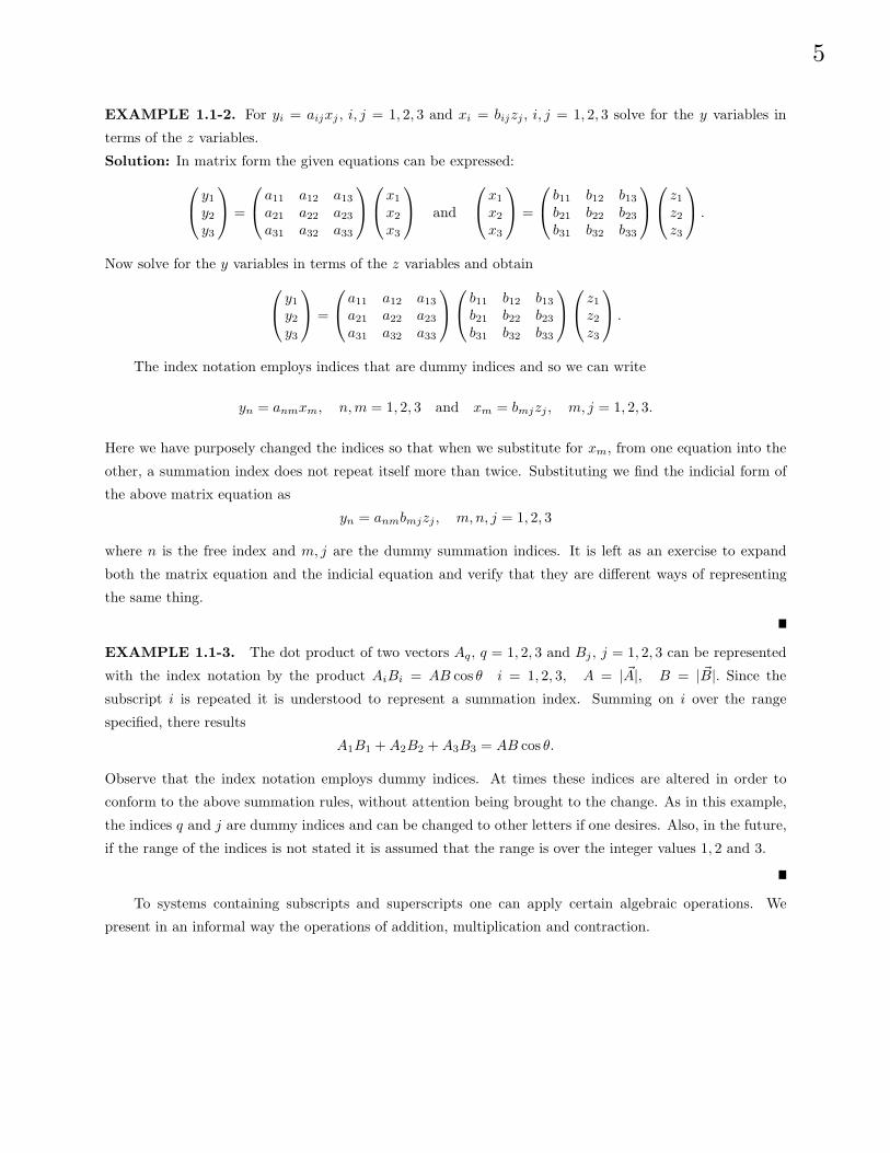
EXAMPLE 1.1-2. For yi = aijxj , i, j = 1, 2, 3 and xi = bijzj , i, j = 1, 2, 3 solve for the y variables in
terms of the z variables.
Solution: In matrix form the given equations can be expressed: y1y2y3
=
a11 a12 a13
a21 a22 a23
a31 a32 a33
x1
x2
x3
and
x1
x2
x3
=
b11 b12 b13b21 b22 b23b31 b32 b33
z1z2z3
.
Now solve for the y variables in terms of the z variables and obtain y1y2y3
=
a11 a12 a13
a21 a22 a23
a31 a32 a33
b11 b12 b13b21 b22 b23b31 b32 b33
z1z2z3
.
The index notation employs indices that are dummy indices and so we can write
yn = anmxm, n,m = 1, 2, 3 and xm = bmjzj , m, j = 1, 2, 3.
Here we have purposely changed the indices so that when we substitute for xm, from one equation into the
other, a summation index does not repeat itself more than twice. Substituting we find the indicial form of
the above matrix equation as
yn = anmbmjzj , m, n, j = 1, 2, 3
where n is the free index and m, j are the dummy summation indices. It is left as an exercise to expand
both the matrix equation and the indicial equation and verify that they are different ways of representing
the same thing.
EXAMPLE 1.1-3. The dot product of two vectors Aq, q = 1, 2, 3 and Bj , j = 1, 2, 3 can be represented
with the index notation by the product AiBi = AB cos θ i = 1, 2, 3, A = | ~A|, B = | ~B|. Since the
subscript i is repeated it is understood to represent a summation index. Summing on i over the range
specified, there results
A1B1 +A2B2 +A3B3 = AB cos θ.
Observe that the index notation employs dummy indices. At times these indices are altered in order to
conform to the above summation rules, without attention being brought to the change. As in this example,
the indices q and j are dummy indices and can be changed to other letters if one desires. Also, in the future,
if the range of the indices is not stated it is assumed that the range is over the integer values 1, 2 and 3.
To systems containing subscripts and superscripts one can apply certain algebraic operations. We
present in an informal way the operations of addition, multiplication and contraction.

6
Addition, Multiplication and Contraction
The algebraic operation of addition or subtraction applies to systems of the same type and order. That
is we can add or subtract like components in systems. For example, the sum of Aijk and Bi
jk is again a
system of the same type and is denoted by Cijk = Ai
jk +Bijk, where like components are added.
The product of two systems is obtained by multiplying each component of the first system with each
component of the second system. Such a product is called an outer product. The order of the resulting
product system is the sum of the orders of the two systems involved in forming the product. For example,
if Aij is a second order system and Bmnl is a third order system, with all indices having the range 1 to N,
then the product system is fifth order and is denoted Cimnlj = Ai
jBmnl. The product system represents N5
terms constructed from all possible products of the components from Aij with the components from Bmnl.
The operation of contraction occurs when a lower index is set equal to an upper index and the summation
convention is invoked. For example, if we have a fifth order system Cimnlj and we set i = j and sum, then
we form the system
Cmnl = Cjmnlj = C1mnl
1 + C2mnl2 + · · ·+ CNmnl
N .
Here the symbol Cmnl is used to represent the third order system that results when the contraction is
performed. Whenever a contraction is performed, the resulting system is always of order 2 less than the
original system. Under certain special conditions it is permissible to perform a contraction on two lower case
indices. These special conditions will be considered later in the section.
The above operations will be more formally defined after we have explained what tensors are.
The e-permutation symbol and Kronecker delta
Two symbols that are used quite frequently with the indicial notation are the e-permutation symbol
and the Kronecker delta. The e-permutation symbol is sometimes referred to as the alternating tensor. The
e-permutation symbol, as the name suggests, deals with permutations. A permutation is an arrangement of
things. When the order of the arrangement is changed, a new permutation results. A transposition is an
interchange of two consecutive terms in an arrangement. As an example, let us change the digits 1 2 3 to
3 2 1 by making a sequence of transpositions. Starting with the digits in the order 1 2 3 we interchange 2 and
3 (first transposition) to obtain 1 3 2. Next, interchange the digits 1 and 3 ( second transposition) to obtain
3 1 2. Finally, interchange the digits 1 and 2 (third transposition) to achieve 3 2 1. Here the total number
of transpositions of 1 2 3 to 3 2 1 is three, an odd number. Other transpositions of 1 2 3 to 3 2 1 can also be
written. However, these are also an odd number of transpositions.

7
EXAMPLE 1.1-4. The total number of possible ways of arranging the digits 1 2 3 is six. We have
three choices for the first digit. Having chosen the first digit, there are only two choices left for the second
digit. Hence the remaining number is for the last digit. The product (3)(2)(1) = 3! = 6 is the number of
permutations of the digits 1, 2 and 3. These six permutations are
1 2 3 even permutation
1 3 2 odd permutation
3 1 2 even permutation
3 2 1 odd permutation
2 3 1 even permutation
2 1 3 odd permutation.
Here a permutation of 1 2 3 is called even or odd depending upon whether there is an even or odd number
of transpositions of the digits. A mnemonic device to remember the even and odd permutations of 123
is illustrated in the figure 1.1-1. Note that even permutations of 123 are obtained by selecting any three
consecutive numbers from the sequence 123123 and the odd permutations result by selecting any three
consecutive numbers from the sequence 321321.
Figure 1.1-1. Permutations of 123.
In general, the number of permutations of n things taken m at a time is given by the relation
P (n,m) = n(n− 1)(n− 2) · · · (n−m+ 1).
By selecting a subset of m objects from a collection of n objects, m ≤ n, without regard to the ordering is
called a combination of n objects taken m at a time. For example, combinations of 3 numbers taken from
the set {1, 2, 3, 4} are (123), (124), (134), (234). Note that ordering of a combination is not considered. That
is, the permutations (123), (132), (231), (213), (312), (321) are considered equal. In general, the number of
combinations of n objects taken m at a time is given by C(n,m) =( nm
)=
n!m!(n−m)!
where(
nm
)are the
binomial coefficients which occur in the expansion
(a+ b)n =n∑
m=0
( nm
)an−mbm.

8
The definition of permutations can be used to define the e-permutation symbol.
Definition: (e-Permutation symbol or alternating tensor)
The e-permutation symbol is defined
eijk...l = eijk...l =
1 if ijk . . . l is an even permutation of the integers 123 . . . n−1 if ijk . . . l is an odd permutation of the integers 123 . . . n0 in all other cases
EXAMPLE 1.1-5. Find e612453.
Solution: To determine whether 612453 is an even or odd permutation of 123456 we write down the given
numbers and below them we write the integers 1 through 6. Like numbers are then connected by a line and
we obtain figure 1.1-2.
Figure 1.1-2. Permutations of 123456.
In figure 1.1-2, there are seven intersections of the lines connecting like numbers. The number of
intersections is an odd number and shows that an odd number of transpositions must be performed. These
results imply e612453 = −1.
Another definition used quite frequently in the representation of mathematical and engineering quantities
is the Kronecker delta which we now define in terms of both subscripts and superscripts.
Definition: (Kronecker delta) The Kronecker delta is defined:
δij = δji =
{1 if i equals j0 if i is different from j

9
EXAMPLE 1.1-6. Some examples of the e−permutation symbol and Kronecker delta are:
e123 = e123 = +1
e213 = e213 = −1
e112 = e112 = 0
δ11 = 1
δ12 = 0
δ13 = 0
δ12 = 0
δ22 = 1
δ32 = 0.
EXAMPLE 1.1-7. When an index of the Kronecker delta δij is involved in the summation convention,
the effect is that of replacing one index with a different index. For example, let aij denote the elements of an
N ×N matrix. Here i and j are allowed to range over the integer values 1, 2, . . . , N. Consider the product
aijδik
where the range of i, j, k is 1, 2, . . . , N. The index i is repeated and therefore it is understood to represent
a summation over the range. The index i is called a summation index. The other indices j and k are free
indices. They are free to be assigned any values from the range of the indices. They are not involved in any
summations and their values, whatever you choose to assign them, are fixed. Let us assign a value of j and
k to the values of j and k. The underscore is to remind you that these values for j and k are fixed and not
to be summed. When we perform the summation over the summation index i we assign values to i from the
range and then sum over these values. Performing the indicated summation we obtain
aijδik = a1jδ1k + a2jδ2k + · · ·+ akjδkk + · · ·+ aNjδNk.
In this summation the Kronecker delta is zero everywhere the subscripts are different and equals one where
the subscripts are the same. There is only one term in this summation which is nonzero. It is that term
where the summation index i was equal to the fixed value k This gives the result
akjδkk = akj
where the underscore is to remind you that the quantities have fixed values and are not to be summed.
Dropping the underscores we write
aijδik = akj
Here we have substituted the index i by k and so when the Kronecker delta is used in a summation process
it is known as a substitution operator. This substitution property of the Kronecker delta can be used to
simplify a variety of expressions involving the index notation. Some examples are:
Bijδjs = Bis
δjkδkm = δjm
eijkδimδjnδkp = emnp.
Some texts adopt the notation that if indices are capital letters, then no summation is to be performed.
For example,
aKJδKK = aKJ
10
as δKK represents a single term because of the capital letters. Another notation which is used to denote no
summation of the indices is to put parenthesis about the indices which are not to be summed. For example,
a(k)jδ(k)(k) = akj ,
since δ(k)(k) represents a single term and the parentheses indicate that no summation is to be performed.
At any time we may employ either the underscore notation, the capital letter notation or the parenthesis
notation to denote that no summation of the indices is to be performed. To avoid confusion altogether, one
can write out parenthetical expressions such as “(no summation on k)”.
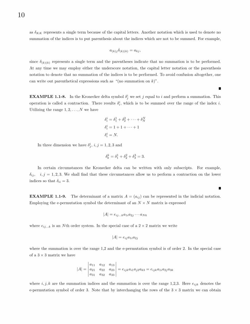
EXAMPLE 1.1-8. In the Kronecker delta symbol δij we set j equal to i and perform a summation. This
operation is called a contraction. There results δii , which is to be summed over the range of the index i.
Utilizing the range 1, 2, . . . , N we have
δii = δ11 + δ22 + · · ·+ δN
N
δii = 1 + 1 + · · ·+ 1
δii = N.
In three dimension we have δij , i, j = 1, 2, 3 and
δkk = δ11 + δ22 + δ33 = 3.
In certain circumstances the Kronecker delta can be written with only subscripts. For example,
δij , i, j = 1, 2, 3. We shall find that these circumstances allow us to perform a contraction on the lower
indices so that δii = 3.
EXAMPLE 1.1-9. The determinant of a matrix A = (aij) can be represented in the indicial notation.
Employing the e-permutation symbol the determinant of an N ×N matrix is expressed
|A| = eij...ka1ia2j · · · aNk
where eij...k is an Nth order system. In the special case of a 2× 2 matrix we write
|A| = eija1ia2j
where the summation is over the range 1,2 and the e-permutation symbol is of order 2. In the special case
of a 3× 3 matrix we have
|A| =∣∣∣∣∣∣a11 a12 a13
a21 a22 a23
a31 a32 a33
∣∣∣∣∣∣ = eijkai1aj2ak3 = eijka1ia2ja3k
where i, j, k are the summation indices and the summation is over the range 1,2,3. Here eijk denotes the
e-permutation symbol of order 3. Note that by interchanging the rows of the 3 × 3 matrix we can obtain

11
more general results. Consider (p, q, r) as some permutation of the integers (1, 2, 3), and observe that the
determinant can be expressed
∆ =
∣∣∣∣∣∣ap1 ap2 ap3
aq1 aq2 aq3
ar1 ar2 ar3
∣∣∣∣∣∣ = eijkapiaqjark.
If (p, q, r) is an even permutation of (1, 2, 3) then ∆ = |A|If (p, q, r) is an odd permutation of (1, 2, 3) then ∆ = −|A|If (p, q, r) is not a permutation of (1, 2, 3) then ∆ = 0.
We can then write
eijkapiaqjark = epqr|A|.
Each of the above results can be verified by performing the indicated summations. A more formal proof of
the above result is given in EXAMPLE 1.1-25, later in this section.
EXAMPLE 1.1-10. The expression eijkBijCi is meaningless since the index i repeats itself more than
twice and the summation convention does not allow this. If you really did want to sum over an index which
occurs more than twice, then one must use a summation sign. For example the above expression would be
writtenn∑
i=1
eijkBijCi.
EXAMPLE 1.1-11.
The cross product of the unit vectors e1, e2, e3 can be represented in the index notation by
ei × ej =
ek if (i, j, k) is an even permutation of (1, 2, 3)− ek if (i, j, k) is an odd permutation of (1, 2, 3)0 in all other cases
This result can be written in the form ei× ej = ekij ek. This later result can be verified by summing on the
index k and writing out all 9 possible combinations for i and j.
EXAMPLE 1.1-12. Given the vectors Ap, p = 1, 2, 3 and Bp, p = 1, 2, 3 the cross product of these two
vectors is a vector Cp, p = 1, 2, 3 with components
Ci = eijkAjBk, i, j, k = 1, 2, 3. (1.1.2)
The quantities Ci represent the components of the cross product vector
~C = ~A× ~B = C1 e1 + C2 e2 + C3 e3.
The equation (1.1.2), which defines the components of ~C, is to be summed over each of the indices which
repeats itself. We have summing on the index k
Ci = eij1AjB1 + eij2AjB2 + eij3AjB3. (1.1.3)

12
We next sum on the index j which repeats itself in each term of equation (1.1.3). This gives
Ci = ei11A1B1 + ei21A2B1 + ei31A3B1
+ ei12A1B2 + ei22A2B2 + ei32A3B2
+ ei13A1B3 + ei23A2B3 + ei33A3B3.
(1.1.4)
Now we are left with i being a free index which can have any of the values of 1, 2 or 3. Letting i = 1, then
letting i = 2, and finally letting i = 3 produces the cross product components
C1 = A2B3 −A3B2
C2 = A3B1 −A1B3
C3 = A1B2 −A2B1.
The cross product can also be expressed in the form ~A × ~B = eijkAjBk ei. This result can be verified by
summing over the indices i,j and k.
EXAMPLE 1.1-13. Show
eijk = −eikj = ejki for i, j, k = 1, 2, 3
Solution: The array i k j represents an odd number of transpositions of the indices i j k and to each
transposition there is a sign change of the e-permutation symbol. Similarly, j k i is an even transposition
of i j k and so there is no sign change of the e-permutation symbol. The above holds regardless of the
numerical values assigned to the indices i, j, k.
The e-δ Identity
An identity relating the e-permutation symbol and the Kronecker delta, which is useful in the simpli-
fication of tensor expressions, is the e-δ identity. This identity can be expressed in different forms. The
subscript form for this identity is
eijkeimn = δjmδkn − δjnδkm, i, j, k,m, n = 1, 2, 3
where i is the summation index and j, k,m, n are free indices. A device used to remember the positions of
the subscripts is given in the figure 1.1-3.
The subscripts on the four Kronecker delta’s on the right-hand side of the e-δ identity then are read
(first)(second)-(outer)(inner).
This refers to the positions following the summation index. Thus, j,m are the first indices after the sum-
mation index and k, n are the second indices after the summation index. The indices j, n are outer indices
when compared to the inner indices k,m as the indices are viewed as written on the left-hand side of the
identity.

13
Figure 1.1-3. Mnemonic device for position of subscripts.
Another form of this identity employs both subscripts and superscripts and has the form
eijkeimn = δjmδ
kn − δj
nδkm. (1.1.5)
One way of proving this identity is to observe the equation (1.1.5) has the free indices j, k,m, n. Each
of these indices can have any of the values of 1, 2 or 3. There are 3 choices we can assign to each of j, k,m
or n and this gives a total of 34 = 81 possible equations represented by the identity from equation (1.1.5).
By writing out all 81 of these equations we can verify that the identity is true for all possible combinations
that can be assigned to the free indices.
An alternate proof of the e− δ identity is to consider the determinant∣∣∣∣∣∣δ11 δ12 δ13δ21 δ22 δ23δ31 δ32 δ33
∣∣∣∣∣∣ =
∣∣∣∣∣∣1 0 00 1 00 0 1
∣∣∣∣∣∣ = 1.
By performing a permutation of the rows of this matrix we can use the permutation symbol and write∣∣∣∣∣∣δi1 δi
2 δi3
δj1 δj
2 δj3
δk1 δk
2 δk3
∣∣∣∣∣∣ = eijk.
By performing a permutation of the columns, we can write∣∣∣∣∣∣δir δi
s δit
δjr δj
s δjt
δkr δk
s δkt
∣∣∣∣∣∣ = eijkerst.
Now perform a contraction on the indices i and r to obtain∣∣∣∣∣∣δii δi
s δit
δji δj
s δjt
δki δk
s δkt
∣∣∣∣∣∣ = eijkeist.
Summing on i we have δii = δ11 + δ22 + δ33 = 3 and expand the determinant to obtain the desired result
δjsδ
kt − δj
t δks = eijkeist.

14
Generalized Kronecker delta
The generalized Kronecker delta is defined by the (n× n) determinant
δij...kmn...p =
∣∣∣∣∣∣∣∣∣
δim δi
n · · · δip
δjm δj
n · · · δjp
......
. . ....
δkm δk
n · · · δkp
∣∣∣∣∣∣∣∣∣.
For example, in three dimensions we can write
δijkmnp =
∣∣∣∣∣∣δim δi
n δip
δjm δj
n δjp
δkm δk
n δkp
∣∣∣∣∣∣ = eijkemnp.
Performing a contraction on the indices k and p we obtain the fourth order system
δrsmn = δrsp
mnp = erspemnp = eprsepmn = δrmδ
sn − δr
nδsm.
As an exercise one can verify that the definition of the e-permutation symbol can also be defined in terms
of the generalized Kronecker delta as
ej1j2j3···jN = δ1 2 3 ···Nj1j2j3···jN
.
Additional definitions and results employing the generalized Kronecker delta are found in the exercises.
In section 1.3 we shall show that the Kronecker delta and epsilon permutation symbol are numerical tensors
which have fixed components in every coordinate system.
Additional Applications of the Indicial Notation
The indicial notation, together with the e− δ identity, can be used to prove various vector identities.
EXAMPLE 1.1-14. Show, using the index notation, that ~A× ~B = − ~B × ~A
Solution: Let~C = ~A× ~B = C1 e1 + C2 e2 + C3 e3 = Ci ei and let
~D = ~B × ~A = D1 e1 +D2 e2 +D3 e3 = Di ei.
We have shown that the components of the cross products can be represented in the index notation by
Ci = eijkAjBk and Di = eijkBjAk.
We desire to show that Di = −Ci for all values of i. Consider the following manipulations: Let Bj = Bsδsj
and Ak = Amδmk and write
Di = eijkBjAk = eijkBsδsjAmδmk (1.1.6)
where all indices have the range 1, 2, 3. In the expression (1.1.6) note that no summation index appears
more than twice because if an index appeared more than twice the summation convention would become
meaningless. By rearranging terms in equation (1.1.6) we have
Di = eijkδsjδmkBsAm = eismBsAm.

15
In this expression the indices s and m are dummy summation indices and can be replaced by any other
letters. We replace s by k and m by j to obtain
Di = eikjAjBk = −eijkAjBk = −Ci.
Consequently, we find that ~D = −~C or ~B × ~A = − ~A× ~B. That is, ~D = Di ei = −Ci ei = −~C.Note 1. The expressions
Ci = eijkAjBk and Cm = emnpAnBp
with all indices having the range 1, 2, 3, appear to be different because different letters are used as sub-
scripts. It must be remembered that certain indices are summed according to the summation convention
and the other indices are free indices and can take on any values from the assigned range. Thus, after
summation, when numerical values are substituted for the indices involved, none of the dummy letters
used to represent the components appear in the answer.
Note 2. A second important point is that when one is working with expressions involving the index notation,
the indices can be changed directly. For example, in the above expression for Di we could have replaced
j by k and k by j simultaneously (so that no index repeats itself more than twice) to obtain
Di = eijkBjAk = eikjBkAj = −eijkAjBk = −Ci.
Note 3. Be careful in switching back and forth between the vector notation and index notation. Observe that a
vector ~A can be represented~A = Ai ei
or its components can be represented
~A · ei = Ai, i = 1, 2, 3.
Do not set a vector equal to a scalar. That is, do not make the mistake of writing ~A = Ai as this is a
misuse of the equal sign. It is not possible for a vector to equal a scalar because they are two entirely
different quantities. A vector has both magnitude and direction while a scalar has only magnitude.
EXAMPLE 1.1-15. Verify the vector identity
~A · ( ~B × ~C) = ~B · (~C × ~A)
Solution: Let~B × ~C = ~D = Di ei where Di = eijkBjCk and let
~C × ~A = ~F = Fi ei where Fi = eijkCjAk
where all indices have the range 1, 2, 3. To prove the above identity, we have
~A · ( ~B × ~C) = ~A · ~D = AiDi = AieijkBjCk
= Bj(eijkAiCk)
= Bj(ejkiCkAi)

16
since eijk = ejki. We also observe from the expression
Fi = eijkCjAk
that we may obtain, by permuting the symbols, the equivalent expression
Fj = ejkiCkAi.
This allows us to write~A · ( ~B × ~C) = BjFj = ~B · ~F = ~B · (~C × ~A)
which was to be shown.
The quantity ~A · ( ~B × ~C) is called a triple scalar product. The above index representation of the triple
scalar product implies that it can be represented as a determinant (See example 1.1-9). We can write
~A · ( ~B × ~C) =
∣∣∣∣∣∣A1 A2 A3
B1 B2 B3
C1 C2 C3
∣∣∣∣∣∣ = eijkAiBjCk
A physical interpretation that can be assigned to this triple scalar product is that its absolute value represents
the volume of the parallelepiped formed by the three noncoplaner vectors ~A, ~B, ~C. The absolute value is
needed because sometimes the triple scalar product is negative. This physical interpretation can be obtained
from an analysis of the figure 1.1-4.
Figure 1.1-4. Triple scalar product and volume

17
In figure 1.1-4 observe that: (i) | ~B × ~C| is the area of the parallelogram PQRS. (ii) the unit vector
en =~B × ~C
| ~B × ~C|
is normal to the plane containing the vectors ~B and ~C. (iii) The dot product
∣∣ ~A · en
∣∣ =∣∣∣∣ ~A ·
~B × ~C
| ~B × ~C|
∣∣∣∣ = h
equals the projection of ~A on en which represents the height of the parallelepiped. These results demonstrate
that ∣∣∣ ~A · ( ~B × ~C)∣∣∣ = | ~B × ~C|h = (area of base)(height) = volume.
EXAMPLE 1.1-16. Verify the vector identity
( ~A× ~B)× (~C × ~D) = ~C( ~D · ~A× ~B)− ~D(~C · ~A× ~B)
Solution: Let ~F = ~A× ~B = Fi ei and ~E = ~C × ~D = Ei ei. These vectors have the components
Fi = eijkAjBk and Em = emnpCnDp
where all indices have the range 1, 2, 3. The vector ~G = ~F × ~E = Gi ei has the components
Gq = eqimFiEm = eqimeijkemnpAjBkCnDp.
From the identity eqim = emqi this can be expressed
Gq = (emqiemnp)eijkAjBkCnDp
which is now in a form where we can use the e− δ identity applied to the term in parentheses to produce
Gq = (δqnδip − δqpδin)eijkAjBkCnDp.
Simplifying this expression we have:
Gq = eijk [(Dpδip)(Cnδqn)AjBk − (Dpδqp)(Cnδin)AjBk]
= eijk [DiCqAjBk −DqCiAjBk]
= Cq [DieijkAjBk]−Dq [CieijkAjBk]
which are the vector components of the vector
~C( ~D · ~A× ~B)− ~D(~C · ~A× ~B).
18
Transformation Equations
Consider two sets of N independent variables which are denoted by the barred and unbarred symbols
xi and xi with i = 1, . . . , N. The independent variables xi, i = 1, . . . , N can be thought of as defining
the coordinates of a point in a N−dimensional space. Similarly, the independent barred variables define a
point in some other N−dimensional space. These coordinates are assumed to be real quantities and are not
complex quantities. Further, we assume that these variables are related by a set of transformation equations.
xi = xi(x1, x2, . . . , xN ) i = 1, . . . , N. (1.1.7)
It is assumed that these transformation equations are independent. A necessary and sufficient condition that
these transformation equations be independent is that the Jacobian determinant be different from zero, that
is
J(x
x) =
∣∣∣∣ ∂xi
∂xj
∣∣∣∣ =
∣∣∣∣∣∣∣∣∣∣
∂x1
∂x1∂x1
∂x2 · · · ∂x1
∂xN
∂x2
∂x1∂x2
∂x2 · · · ∂x2
∂xN
......
. . ....
∂xN
∂x1∂xN
∂x2 · · · ∂xN
∂xN
∣∣∣∣∣∣∣∣∣∣6= 0.
This assumption allows us to obtain a set of inverse relations
xi = xi(x1, x2, . . . , xN ) i = 1, . . . , N, (1.1.8)
where the x′s are determined in terms of the x′s. Throughout our discussions it is to be understood that the
given transformation equations are real and continuous. Further all derivatives that appear in our discussions
are assumed to exist and be continuous in the domain of the variables considered.
EXAMPLE 1.1-17. The following is an example of a set of transformation equations of the form
defined by equations (1.1.7) and (1.1.8) in the case N = 3. Consider the transformation from cylindrical
coordinates (r, α, z) to spherical coordinates (ρ, β, α). From the geometry of the figure 1.1-5 we can find the
transformation equationsr = ρ sinβ
α = α 0 < α < 2π
z = ρ cosβ 0 < β < π
with inverse transformationρ =
√r2 + z2
α = α
β = arctan(r
z)
Now make the substitutions
(x1, x2, x3) = (r, α, z) and (x1, x2, x3) = (ρ, β, α).
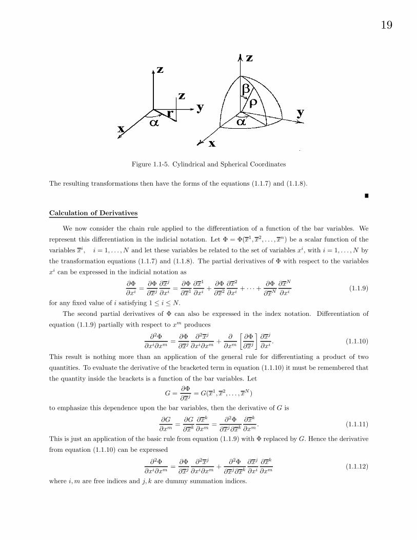
19
Figure 1.1-5. Cylindrical and Spherical Coordinates
The resulting transformations then have the forms of the equations (1.1.7) and (1.1.8).
Calculation of Derivatives
We now consider the chain rule applied to the differentiation of a function of the bar variables. We
represent this differentiation in the indicial notation. Let Φ = Φ(x1, x2, . . . , xn) be a scalar function of the
variables xi, i = 1, . . . , N and let these variables be related to the set of variables xi, with i = 1, . . . , N by
the transformation equations (1.1.7) and (1.1.8). The partial derivatives of Φ with respect to the variables
xi can be expressed in the indicial notation as
∂Φ∂xi
=∂Φ∂xj
∂xj
∂xi=
∂Φ∂x1
∂x1
∂xi+∂Φ∂x2
∂x2
∂xi+ · · ·+ ∂Φ
∂xN
∂xN
∂xi(1.1.9)
for any fixed value of i satisfying 1 ≤ i ≤ N.
The second partial derivatives of Φ can also be expressed in the index notation. Differentiation of
equation (1.1.9) partially with respect to xm produces
∂2Φ∂xi∂xm
=∂Φ∂xj
∂2xj
∂xi∂xm+
∂
∂xm
[∂Φ∂xj
]∂xj
∂xi. (1.1.10)
This result is nothing more than an application of the general rule for differentiating a product of two
quantities. To evaluate the derivative of the bracketed term in equation (1.1.10) it must be remembered that
the quantity inside the brackets is a function of the bar variables. Let
G =∂Φ∂xj = G(x1, x2, . . . , xN )
to emphasize this dependence upon the bar variables, then the derivative of G is
∂G
∂xm=
∂G
∂xk
∂xk
∂xm=
∂2Φ∂xj∂xk
∂xk
∂xm. (1.1.11)
This is just an application of the basic rule from equation (1.1.9) with Φ replaced by G. Hence the derivative
from equation (1.1.10) can be expressed
∂2Φ∂xi∂xm
=∂Φ∂xj
∂2xj
∂xi∂xm+
∂2Φ∂xj∂xk
∂xj
∂xi
∂xk
∂xm(1.1.12)
where i,m are free indices and j, k are dummy summation indices.
20
EXAMPLE 1.1-18. Let Φ = Φ(r, θ) where r, θ are polar coordinates related to the Cartesian coordinates
(x, y) by the transformation equations x = r cos θ y = r sin θ. Find the partial derivatives∂Φ∂x
and∂2Φ∂x2
Solution: The partial derivative of Φ with respect to x is found from the relation (1.1.9) and can be written
∂Φ∂x
=∂Φ∂r
∂r
∂x+∂Φ∂θ
∂θ
∂x. (1.1.13)
The second partial derivative is obtained by differentiating the first partial derivative. From the product
rule for differentiation we can write
∂2Φ∂x2
=∂Φ∂r
∂2r
∂x2+∂r
∂x
∂
∂x
[∂Φ∂r
]+∂Φ∂θ
∂2θ
∂x2+∂θ
∂x
∂
∂x
[∂Φ∂θ
]. (1.1.14)
To further simplify (1.1.14) it must be remembered that the terms inside the brackets are to be treated as
functions of the variables r and θ and that the derivative of these terms can be evaluated by reapplying the
basic rule from equation (1.1.13) with Φ replaced by ∂Φ∂r and then Φ replaced by ∂Φ
∂θ . This gives
∂2Φ∂x2
=∂Φ∂r
∂2r
∂x2+∂r
∂x
[∂2Φ∂r2
∂r
∂x+
∂2Φ∂r∂θ
∂θ
∂x
]
+∂Φ∂θ
∂2θ
∂x2+∂θ
∂x
[∂2Φ∂θ∂r
∂r
∂x+∂2Φ∂θ2
∂θ
∂x
].
(1.1.15)
From the transformation equations we obtain the relations r2 = x2 +y2 and tan θ =y
xand from
these relations we can calculate all the necessary derivatives needed for the simplification of the equations
(1.1.13) and (1.1.15). These derivatives are:
2r∂r
∂x= 2x or
∂r
∂x=x
r= cos θ
sec2 θ∂θ
∂x= − y
x2or
∂θ
∂x= − y
r2= − sin θ
r
∂2r
∂x2= − sin θ
∂θ
∂x=
sin2 θ
r
∂2θ
∂x2=−r cos θ ∂θ
∂x + sin θ ∂r∂x
r2=
2 sin θ cos θr2
.
Therefore, the derivatives from equations (1.1.13) and (1.1.15) can be expressed in the form
∂Φ∂x
=∂Φ∂r
cos θ − ∂Φ∂θ
sin θr
∂2Φ∂x2
=∂Φ∂r
sin2 θ
r+ 2
∂Φ∂θ
sin θ cos θr2
+∂2Φ∂r2
cos2 θ − 2∂2Φ∂r∂θ
cos θ sin θr
+∂2Φ∂θ2
sin2 θ
r2.
By letting x1 = r, x2 = θ, x1 = x, x2 = y and performing the indicated summations in the equations (1.1.9)
and (1.1.12) there is produced the same results as above.
Vector Identities in Cartesian Coordinates
Employing the substitutions x1 = x, x2 = y, x3 = z, where superscript variables are employed and
denoting the unit vectors in Cartesian coordinates by e1, e2, e3, we illustrated how various vector operations
are written by using the index notation.

21
Gradient. In Cartesian coordinates the gradient of a scalar field is
gradφ =∂φ
∂xe1 +
∂φ
∂ye2 +
∂φ
∂ze3.
The index notation focuses attention only on the components of the gradient. In Cartesian coordinates these
components are represented using a comma subscript to denote the derivative
ej · gradφ = φ,j =∂φ
∂xj, j = 1, 2, 3.
The comma notation will be discussed in section 4. For now we use it to denote derivatives. For example
φ ,j =∂φ
∂xj, φ ,jk =
∂2φ
∂xj∂xk, etc.
Divergence. In Cartesian coordinates the divergence of a vector field ~A is a scalar field and can be
represented
∇ · ~A = div ~A =∂A1
∂x+∂A2
∂y+∂A3
∂z.
Employing the summation convention and index notation, the divergence in Cartesian coordinates can be
represented
∇ · ~A = div ~A = Ai,i =∂Ai
∂xi=∂A1
∂x1+∂A2
∂x2+∂A3
∂x3
where i is the dummy summation index.
Curl. To represent the vector ~B = curl ~A = ∇ × ~A in Cartesian coordinates, we note that the index
notation focuses attention only on the components of this vector. The components Bi, i = 1, 2, 3 of ~B can
be represented
Bi = ei · curl ~A = eijkAk,j , for i, j, k = 1, 2, 3
where eijk is the permutation symbol introduced earlier and Ak,j = ∂Ak
∂xj . To verify this representation of the
curl ~A we need only perform the summations indicated by the repeated indices. We have summing on j that
Bi = ei1kAk,1 + ei2kAk,2 + ei3kAk,3.
Now summing each term on the repeated index k gives us
Bi = ei12A2,1 + ei13A3,1 + ei21A1,2 + ei23A3,2 + ei31A1,3 + ei32A2,3
Here i is a free index which can take on any of the values 1, 2 or 3. Consequently, we have
For i = 1, B1 = A3,2 −A2,3 =∂A3
∂x2− ∂A2
∂x3
For i = 2, B2 = A1,3 −A3,1 =∂A1
∂x3− ∂A3
∂x1
For i = 3, B3 = A2,1 −A1,2 =∂A2
∂x1− ∂A1
∂x2
which verifies the index notation representation of curl ~A in Cartesian coordinates.

22
Other Operations. The following examples illustrate how the index notation can be used to represent
additional vector operators in Cartesian coordinates.
1. In index notation the components of the vector ( ~B · ∇) ~A are
{( ~B · ∇) ~A} · ep = Ap,qBq p, q = 1, 2, 3
This can be verified by performing the indicated summations. We have by summing on the repeated
index q
Ap,qBq = Ap,1B1 +Ap,2B2 +Ap,3B3.
The index p is now a free index which can have any of the values 1, 2 or 3. We have:
for p = 1, A1,qBq = A1,1B1 +A1,2B2 +A1,3B3
=∂A1
∂x1B1 +
∂A1
∂x2B2 +
∂A1
∂x3B3
for p = 2, A2,qBq = A2,1B1 +A2,2B2 +A2,3B3
=∂A2
∂x1B1 +
∂A2
∂x2B2 +
∂A2
∂x3B3
for p = 3, A3,qBq = A3,1B1 +A3,2B2 +A3,3B3
=∂A3
∂x1B1 +
∂A3
∂x2B2 +
∂A3
∂x3B3
2. The scalar ( ~B · ∇)φ has the following form when expressed in the index notation:
( ~B · ∇)φ = Biφ,i = B1φ,1 +B2φ,2 +B3φ,3
= B1∂φ
∂x1+B2
∂φ
∂x2+B3
∂φ
∂x3.
3. The components of the vector ( ~B ×∇)φ is expressed in the index notation by
ei ·[( ~B ×∇)φ
]= eijkBjφ,k.
This can be verified by performing the indicated summations and is left as an exercise.
4. The scalar ( ~B ×∇) · ~A may be expressed in the index notation. It has the form
( ~B ×∇) · ~A = eijkBjAi,k.
This can also be verified by performing the indicated summations and is left as an exercise.
5. The vector components of ∇2 ~A in the index notation are represented
ep · ∇2 ~A = Ap,qq .
The proof of this is left as an exercise.
23
EXAMPLE 1.1-19. In Cartesian coordinates prove the vector identity
curl (f ~A) = ∇× (f ~A) = (∇f)× ~A+ f(∇× ~A).
Solution: Let ~B = curl (f ~A) and write the components as
Bi = eijk(fAk),j
= eijk [fAk,j + f,jAk]
= feijkAk,j + eijkf,jAk.
This index form can now be expressed in the vector form
~B = curl (f ~A) = f(∇× ~A) + (∇f)× ~A
EXAMPLE 1.1-20. Prove the vector identity ∇ · ( ~A+ ~B) = ∇ · ~A+∇ · ~BSolution: Let ~A+ ~B = ~C and write this vector equation in the index notation as Ai + Bi = Ci. We then
have
∇ · ~C = Ci,i = (Ai +Bi),i = Ai,i +Bi,i = ∇ · ~A+∇ · ~B.
EXAMPLE 1.1-21. In Cartesian coordinates prove the vector identity ( ~A · ∇)f = ~A · ∇fSolution: In the index notation we write
( ~A · ∇)f = Aif,i = A1f,1 +A2f,2 +A3f,3
= A1∂f
∂x1+A2
∂f
∂x2+A3
∂f
∂x3= ~A · ∇f.
EXAMPLE 1.1-22. In Cartesian coordinates prove the vector identity
∇× ( ~A× ~B) = ~A(∇ · ~B)− ~B(∇ · ~A) + ( ~B · ∇) ~A− ( ~A · ∇) ~B
Solution: The pth component of the vector ∇× ( ~A× ~B) is
ep · [∇× ( ~A× ~B)] = epqk[ekjiAjBi],q
= epqkekjiAjBi,q + epqkekjiAj,qBi
By applying the e− δ identity, the above expression simplifies to the desired result. That is,
ep · [∇× ( ~A× ~B)] = (δpjδqi − δpiδqj)AjBi,q + (δpjδqi − δpiδqj)Aj,qBi
= ApBi,i −AqBp,q +Ap,qBq −Aq,qBp
In vector form this is expressed
∇× ( ~A× ~B) = ~A(∇ · ~B)− ( ~A · ∇) ~B + ( ~B · ∇) ~A− ~B(∇ · ~A)

24
EXAMPLE 1.1-23. In Cartesian coordinates prove the vector identity ∇× (∇× ~A) = ∇(∇ · ~A)−∇2 ~A
Solution: We have for the ith component of ∇× ~A is given by ei · [∇× ~A] = eijkAk,j and consequently the
pth component of ∇× (∇× ~A) is
ep · [∇× (∇× ~A)] = epqr[erjkAk,j ],q
= epqrerjkAk,jq .
The e− δ identity produces
ep · [∇× (∇× ~A)] = (δpjδqk − δpkδqj)Ak,jq
= Ak,pk −Ap,qq .
Expressing this result in vector form we have ∇× (∇× ~A) = ∇(∇ · ~A)−∇2 ~A.
Indicial Form of Integral Theorems
The divergence theorem, in both vector and indicial notation, can be written∫∫∫V
div · ~F dτ =∫∫
S
~F · n dσ∫
V
Fi,i dτ =∫
S
Fini dσ i = 1, 2, 3 (1.1.16)
where ni are the direction cosines of the unit exterior normal to the surface, dτ is a volume element and dσ
is an element of surface area. Note that in using the indicial notation the volume and surface integrals are
to be extended over the range specified by the indices. This suggests that the divergence theorem can be
applied to vectors in n−dimensional spaces.
The vector form and indicial notation for the Stokes theorem are∫∫S
(∇× ~F ) · n dσ =∫
C
~F · d~r∫
S
eijkFk,jni dσ =∫
C
Fi dxi i, j, k = 1, 2, 3 (1.1.17)
and the Green’s theorem in the plane, which is a special case of the Stoke’s theorem, can be expressed
∫∫ (∂F2
∂x− ∂F1
∂y
)dxdy =
∫C
F1 dx+ F2 dy
∫S
e3jkFk,j dS =∫
C
Fi dxi i, j, k = 1, 2 (1.1.18)
Other forms of the above integral theorems are∫∫∫V
∇φdτ =∫∫
S
φ n dσ
obtained from the divergence theorem by letting ~F = φ~C where ~C is a constant vector. By replacing ~F by~F × ~C in the divergence theorem one can derive∫∫∫
V
(∇× ~F
)dτ = −
∫∫S
~F × ~n dσ.
In the divergence theorem make the substitution ~F = φ∇ψ to obtain∫∫∫V
[(φ∇2ψ + (∇φ) · (∇ψ)
]dτ =
∫∫S
(φ∇ψ) · n dσ.

25
The Green’s identity ∫∫∫V
(φ∇2ψ − ψ∇2φ
)dτ =
∫∫S
(φ∇ψ − ψ∇φ) · n dσ
is obtained by first letting ~F = φ∇ψ in the divergence theorem and then letting ~F = ψ∇φ in the divergence
theorem and then subtracting the results.
Determinants, Cofactors
For A = (aij), i, j = 1, . . . , n an n× n matrix, the determinant of A can be written as
detA = |A| = ei1i2i3...ina1i1a2i2a3i3 . . . anin .
This gives a summation of the n! permutations of products formed from the elements of the matrix A. The
result is a single number called the determinant of A.
EXAMPLE 1.1-24. In the case n = 2 we have
|A| =∣∣∣∣ a11 a12
a21 a22
∣∣∣∣ = enma1na2m
= e1ma11a2m + e2ma12a2m
= e12a11a22 + e21a12a21
= a11a22 − a12a21
EXAMPLE 1.1-25. In the case n = 3 we can use either of the notations
A =
a11 a12 a13
a21 a22 a23
a31 a32 a33
or A =
a1
1 a12 a1
3
a21 a2
2 a23
a31 a3
2 a33
and represent the determinant of A in any of the forms
detA = eijka1ia2ja3k
detA = eijkai1aj2ak3
detA = eijkai1a
j2a
k3
detA = eijka1i a
2ja
3k.
These represent row and column expansions of the determinant.
An important identity results if we examine the quantity Brst = eijkaira
jsa
kt . It is an easy exercise to
change the dummy summation indices and rearrange terms in this expression. For example,
Brst = eijkaira
jsa
kt = ekjia
kra
jsa
it = ekjia
ita
jsa
kr = −eijka
ita
jsa
kr = −Btsr,
and by considering other permutations of the indices, one can establish that Brst is completely skew-
symmetric. In the exercises it is shown that any third order completely skew-symmetric system satisfies
Brst = B123erst. But B123 = detA and so we arrive at the identity
Brst = eijkaira
jsa
kt = |A|erst.

26
Other forms of this identity are
eijkari a
sja
tk = |A|erst and eijkairajsakt = |A|erst. (1.1.19)
Consider the representation of the determinant
|A| =∣∣∣∣∣∣a11 a1
2 a13
a21 a2
2 a23
a31 a3
2 a33
∣∣∣∣∣∣by use of the indicial notation. By column expansions, this determinant can be represented
|A| = erstar1a
s2a
t3 (1.1.20)
and if one uses row expansions the determinant can be expressed as
|A| = eijka1i a
2ja
3k. (1.1.21)
Define Aim as the cofactor of the element am
i in the determinant |A|. From the equation (1.1.20) the cofactor
of ar1 is obtained by deleting this element and we find
A1r = ersta
s2a
t3. (1.1.22)
The result (1.1.20) can then be expressed in the form
|A| = ar1A
1r = a1
1A11 + a2
1A12 + a3
1A13. (1.1.23)
That is, the determinant |A| is obtained by multiplying each element in the first column by its corresponding
cofactor and summing the result. Observe also that from the equation (1.1.20) we find the additional
cofactors
A2s = ersta
r1a
t3 and A3
t = erstar1a
s2. (1.1.24)
Hence, the equation (1.1.20) can also be expressed in one of the forms
|A| = as2A
2s = a1
2A21 + a2
2A22 + a3
2A23
|A| = at3A
3t = a1
3A31 + a2
3A32 + a3
3A33
The results from equations (1.1.22) and (1.1.24) can be written in a slightly different form with the indicial
notation. From the notation for a generalized Kronecker delta defined by
eijkelmn = δijklmn,
the above cofactors can be written in the form
A1r = e123ersta
s2a
t3 =
12!e1jkersta
sja
tk =
12!δ1jkrst a
sja
tk
A2r = e123esrta
s1a
t3 =
12!e2jkersta
sja
tk =
12!δ2jkrst a
sja
tk
A3r = e123etsra
t1a
s2 =
12!e3jkersta
sja
tk =
12!δ3jkrst a
sja
tk.

27
These cofactors are then combined into the single equation
Air =
12!δijkrsta
sja
tk (1.1.25)
which represents the cofactor of ari . When the elements from any row (or column) are multiplied by their
corresponding cofactors, and the results summed, we obtain the value of the determinant. Whenever the
elements from any row (or column) are multiplied by the cofactor elements from a different row (or column),
and the results summed, we get zero. This can be illustrated by considering the summation
amr A
im =
12!δijkmsta
sja
tka
mr =
12!eijkemsta
mr a
sja
tk
=12!eijkerjk|A| = 1
2!δijkrjk|A| = δi
r|A|
Here we have used the e− δ identity to obtain
δijkrjk = eijkerjk = ejikejrk = δi
rδkk − δi
kδkr = 3δi
r − δir = 2δi
r
which was used to simplify the above result.
As an exercise one can show that an alternate form of the above summation of elements by its cofactors
is
armA
mi = |A|δr
i .
EXAMPLE 1.1-26. In N-dimensions the quantity δj1j2...jN
k1k2...kNis called a generalized Kronecker delta. It
can be defined in terms of permutation symbols as
ej1j2...jN ek1k2...kN = δj1j2...jN
k1k2...kN(1.1.26)
Observe that
δj1j2...jN
k1k2...kNek1k2...kN = (N !) ej1j2...jN
This follows because ek1k2...kN is skew-symmetric in all pairs of its superscripts. The left-hand side denotes
a summation of N ! terms. The first term in the summation has superscripts j1j2 . . . jN and all other terms
have superscripts which are some permutation of this ordering with minus signs associated with those terms
having an odd permutation. Because ej1j2...jN is completely skew-symmetric we find that all terms in the
summation have the value +ej1j2...jN . We thus obtain N ! of these terms.

28
EXERCISE 1.1
I 1. Simplify each of the following by employing the summation property of the Kronecker delta. Perform
sums on the summation indices only if your are unsure of the result.
(a) eijkδkn
(b) eijkδisδjm
(c) eijkδisδjmδkn
(d) aijδin
(e) δijδjn
(f) δijδjnδni
I 2. Simplify and perform the indicated summations over the range 1, 2, 3
(a) δii
(b) δijδij
(c) eijkAiAjAk
(d) eijkeijk
(e) eijkδjk
(f) AiBjδji −BmAnδmn
I 3. Express each of the following in index notation. Be careful of the notation you use. Note that ~A = Ai
is an incorrect notation because a vector can not equal a scalar. The notation ~A · ei = Ai should be used to
express the ith component of a vector.
(a) ~A · ( ~B × ~C)
(b) ~A× ( ~B × ~C)
(c) ~B( ~A · ~C)
(d) ~B( ~A · ~C)− ~C( ~A · ~B)
I 4. Show the e permutation symbol satisfies: (a) eijk = ejki = ekij (b) eijk = −ejik = −eikj = −ekji
I 5. Use index notation to verify the vector identity ~A× ( ~B × ~C) = ~B( ~A · ~C)− ~C( ~A · ~B)
I 6. Let yi = aijxj and xm = aimzi where the range of the indices is 1, 2
(a) Solve for yi in terms of zi using the indicial notation and check your result
to be sure that no index repeats itself more than twice.
(b) Perform the indicated summations and write out expressions
for y1, y2 in terms of z1, z2
(c) Express the above equations in matrix form. Expand the matrix
equations and check the solution obtained in part (b).
I 7. Use the e− δ identity to simplify (a) eijkejik (b) eijkejki
I 8. Prove the following vector identities:
(a) ~A · ( ~B × ~C) = ~B · (~C × ~A) = ~C · ( ~A× ~B) triple scalar product
(b) ( ~A× ~B)× ~C = ~B( ~A · ~C)− ~A( ~B · ~C)
I 9. Prove the following vector identities:
(a) ( ~A× ~B) · (~C × ~D) = ( ~A · ~C)( ~B · ~D)− ( ~A · ~D)( ~B · ~C)
(b) ~A× ( ~B × ~C) + ~B × (~C × ~A) + ~C × ( ~A× ~B) = ~0
(c) ( ~A× ~B)× (~C × ~D) = ~B( ~A · ~C × ~D)− ~A( ~B · ~C × ~D)
29
I 10. For ~A = (1,−1, 0) and ~B = (4,−3, 2) find using the index notation,
(a) Ci = eijkAjBk, i = 1, 2, 3
(b) AiBi
(c) What do the results in (a) and (b) represent?
I 11. Represent the differential equationsdy1dt
= a11y1 + a12y2 anddy2dt
= a21y1 + a22y2
using the index notation.
I 12.
Let Φ = Φ(r, θ) where r, θ are polar coordinates related to Cartesian coordinates (x, y) by the transfor-
mation equations x = r cos θ and y = r sin θ.
(a) Find the partial derivatives∂Φ∂y
, and∂2Φ∂y2
(b) Combine the result in part (a) with the result from EXAMPLE 1.1-18 to calculate the Laplacian
∇2Φ =∂2Φ∂x2
+∂2Φ∂y2
in polar coordinates.
I 13. (Index notation) Let a11 = 3, a12 = 4, a21 = 5, a22 = 6.
Calculate the quantity C = aijaij , i, j = 1, 2.
I 14. Show the moments of inertia Iij defined by
I11 =∫∫∫
R
(y2 + z2)ρ(x, y, z) dτ
I22 =∫∫∫
R
(x2 + z2)ρ(x, y, z) dτ
I33 =∫∫∫
R
(x2 + y2)ρ(x, y, z) dτ
I23 = I32 = −∫∫∫
R
yzρ(x, y, z) dτ
I12 = I21 = −∫∫∫
R
xyρ(x, y, z) dτ
I13 = I31 = −∫∫∫
R
xzρ(x, y, z) dτ,
can be represented in the index notation as Iij =∫∫∫
R
(xmxmδij − xixj
)ρ dτ, where ρ is the density,
x1 = x, x2 = y, x3 = z and dτ = dxdydz is an element of volume.
I 15. Determine if the following relation is true or false. Justify your answer.
ei · ( ej × ek) = ( ei × ej) · ek = eijk, i, j, k = 1, 2, 3.
Hint: Let em = (δ1m, δ2m, δ3m).
I 16. Without substituting values for i, l = 1, 2, 3 calculate all nine terms of the given quantities
(a) Bil = (δijAk + δi
kAj)ejkl (b) Ail = (δmi B
k + δki B
m)emlk
I 17. Let Amnxmyn = 0 for arbitrary xi and yi, i = 1, 2, 3, and show that Aij = 0 for all values of i, j.

30
I 18.
(a) For amn,m, n = 1, 2, 3 skew-symmetric, show that amnxmxn = 0.
(b) Let amnxmxn = 0, m, n = 1, 2, 3 for all values of xi, i = 1, 2, 3 and show that amn must be skew-
symmetric.
I 19. Let A and B denote 3× 3 matrices with elements aij and bij respectively. Show that if C = AB is a
matrix product, then det(C) = det(A) · det(B).
Hint: Use the result from example 1.1-9.
I 20.
(a) Let u1, u2, u3 be functions of the variables s1, s2, s3. Further, assume that s1, s2, s3 are in turn each
functions of the variables x1, x2, x3. Let∣∣∣∣∂um
∂xn
∣∣∣∣ =∂(u1, u2, u3)∂(x1, x2, x3)
denote the Jacobian of the u′s with
respect to the x′s. Show that ∣∣∣∣ ∂ui
∂xm
∣∣∣∣ =∣∣∣∣∂ui
∂sj
∂sj
∂xm
∣∣∣∣ =∣∣∣∣∂ui
∂sj
∣∣∣∣ ·∣∣∣∣ ∂sj
∂xm
∣∣∣∣ .(b) Note that
∂xi
∂xj
∂xj
∂xm=
∂xi
∂xm= δi
m and show that J(xx)·J( x
x ) = 1, where J(xx ) is the Jacobian determinant
of the transformation (1.1.7).
I 21. A third order system a`mn with `,m, n = 1, 2, 3 is said to be symmetric in two of its subscripts if the
components are unaltered when these subscripts are interchanged. When a`mn is completely symmetric then
a`mn = am`n = a`nm = amn` = anm` = an`m. Whenever this third order system is completely symmetric,
then: (i) How many components are there? (ii) How many of these components are distinct?
Hint: Consider the three cases (i) ` = m = n (ii) ` = m 6= n (iii) ` 6= m 6= n.
I 22. A third order system b`mn with `,m, n = 1, 2, 3 is said to be skew-symmetric in two of its subscripts
if the components change sign when the subscripts are interchanged. A completely skew-symmetric third
order system satisfies b`mn = −bm`n = bmn` = −bnm` = bn`m = −b`nm. (i) How many components does
a completely skew-symmetric system have? (ii) How many of these components are zero? (iii) How many
components can be different from zero? (iv) Show that there is one distinct component b123 and that
b`mn = e`mnb123.
Hint: Consider the three cases (i) ` = m = n (ii) ` = m 6= n (iii) ` 6= m 6= n.
I 23. Let i, j, k = 1, 2, 3 and assume that eijkσjk = 0 for all values of i. What does this equation tell you
about the values σij , i, j = 1, 2, 3?
I 24. Assume that Amn and Bmn are symmetric for m,n = 1, 2, 3. Let Amnxmxn = Bmnx
mxn for arbitrary
values of xi, i = 1, 2, 3, and show that Aij = Bij for all values of i and j.
I 25. Assume Bmn is symmetric and Bmnxmxn = 0 for arbitrary values of xi, i = 1, 2, 3, show that Bij = 0.

31
I 26. (Generalized Kronecker delta) Define the generalized Kronecker delta as the n×n determinant
δij...kmn...p =
∣∣∣∣∣∣∣∣∣
δim δi
n · · · δip
δjm δj
n · · · δjp
......
. . ....
δkm δk
n · · · δkp
∣∣∣∣∣∣∣∣∣where δr
s is the Kronecker delta.
(a) Show eijk = δ123ijk
(b) Show eijk = δijk123
(c) Show δijmn = eijemn
(d) Define δrsmn = δrsp
mnp (summation on p)
and show δrsmn = δr
mδsn − δr
nδsm
Note that by combining the above result with the result from part (c)
we obtain the two dimensional form of the e− δ identity ersemn = δrmδ
sn − δr
nδsm.
(e) Define δrm = 1
2δrnmn (summation on n) and show δrst
pst = 2δrp
(f) Show δrstrst = 3!
I 27. Let Air denote the cofactor of ar
i in the determinant
∣∣∣∣∣∣a11 a1
2 a13
a21 a2
2 a23
a31 a3
2 a33
∣∣∣∣∣∣ as given by equation (1.1.25).
(a) Show erstAir = eijkas
jatk (b) Show erstA
ri = eijka
jsa
kt
I 28. (a) Show that if Aijk = Ajik , i, j, k = 1, 2, 3 there is a total of 27 elements, but only 18 are distinct.
(b) Show that for i, j, k = 1, 2, . . . , N there are N3 elements, but only N2(N + 1)/2 are distinct.
I 29. Let aij = BiBj for i, j = 1, 2, 3 where B1, B2, B3 are arbitrary constants. Calculate det(aij) = |A|.
I 30.(a) For A = (aij), i, j = 1, 2, 3, show |A| = eijkai1aj2ak3.
(b) For A = (aij), i, j = 1, 2, 3, show |A| = eijka
i1a
j2a
k3 .
(c) For A = (aij), i, j = 1, 2, 3, show |A| = eijka1
i a2ja
3k.
(d) For I = (δij), i, j = 1, 2, 3, show |I| = 1.
I 31. Let |A| = eijkai1aj2ak3 and define Aim as the cofactor of aim. Show the determinant can be
expressed in any of the forms:
(a) |A| = Ai1ai1 where Ai1 = eijkaj2ak3
(b) |A| = Aj2aj2 where Ai2 = ejikaj1ak3
(c) |A| = Ak3ak3 where Ai3 = ejkiaj1ak2

32
I 32. Show the results in problem 31 can be written in the forms:
Ai1 =12!e1steijkajsakt, Ai2 =
12!e2steijkajsakt, Ai3 =
12!e3steijkajsakt, or Aim =
12!emsteijkajsakt
I 33. Use the results in problems 31 and 32 to prove that apmAim = |A|δip.
I 34. Let (aij) =
1 2 1
1 0 32 3 2
and calculate C = aijaij , i, j = 1, 2, 3.
I 35. Leta111 = −1, a112 = 3, a121 = 4, a122 = 2
a211 = 1, a212 = 5, a221 = 2, a222 = −2
and calculate the quantity C = aijkaijk , i, j, k = 1, 2.
I 36. Leta1111 = 2, a1112 = 1, a1121 = 3, a1122 = 1
a1211 = 5, a1212 = −2, a1221 = 4, a1222 = −2
a2111 = 1, a2112 = 0, a2121 = −2, a2122 = −1
a2211 = −2, a2212 = 1, a2221 = 2, a2222 = 2
and calculate the quantity C = aijklaijkl, i, j, k, l = 1, 2.
I 37. Simplify the expressions:
(a) (Aijkl +Ajkli +Aklij +Alijk)xixjxkxl
(b) (Pijk + Pjki + Pkij)xixjxk
(c)∂xi
∂xj
(d) aij∂2xi
∂xt∂xs
∂xj
∂xr − ami∂2xm
∂xs∂xt
∂xi
∂xr
I 38. Let g denote the determinant of the matrix having the components gij , i, j = 1, 2, 3. Show that
(a) g erst =
∣∣∣∣∣∣g1r g1s g1t
g2r g2s g2t
g3r g3s g3t
∣∣∣∣∣∣ (b) g ersteijk =
∣∣∣∣∣∣gir gis git
gjr gjs gjt
gkr gks gkt
∣∣∣∣∣∣
I 39. Show that eijkemnp = δijkmnp =
∣∣∣∣∣∣δim δi
n δip
δjm δj
n δjp
δkm δk
n δkp
∣∣∣∣∣∣I 40. Show that eijkemnpA
mnp = Aijk −Aikj +Akij −Ajik +Ajki −Akji
Hint: Use the results from problem 39.
I 41. Show that
(a) eijeij = 2!
(b) eijkeijk = 3!
(c) eijkleijkl = 4!
(d) Guess at the result ei1i2...in ei1i2...in
33
I 42. Determine if the following statement is true or false. Justify your answer. eijkAiBjCk = eijkAjBkCi.
I 43. Let aij , i, j = 1, 2 denote the components of a 2× 2 matrix A, which are functions of time t.
(a) Expand both |A| = eijai1aj2 and |A| =∣∣∣∣ a11 a12
a21 a22
∣∣∣∣ to verify that these representations are the same.
(b) Verify the equivalence of the derivative relations
d|A|dt
= eijdai1
dtaj2 + eijai1
daj2
dtand
d|A|dt
=∣∣∣∣ da11
dtda12dt
a21 a22
∣∣∣∣ +∣∣∣∣ a11 a12
da21dt
da22dt
∣∣∣∣(c) Let aij , i, j = 1, 2, 3 denote the components of a 3× 3 matrix A, which are functions of time t. Develop
appropriate relations, expand them and verify, similar to parts (a) and (b) above, the representation of
a determinant and its derivative.
I 44. For f = f(x1, x2, x3) and φ = φ(f) differentiable scalar functions, use the indicial notation to find a
formula to calculate gradφ .
I 45. Use the indicial notation to prove (a) ∇×∇φ = ~0 (b) ∇ · ∇ × ~A = 0
I 46. If Aij is symmetric and Bij is skew-symmetric, i, j = 1, 2, 3, then calculate C = AijBij .
I 47. Assume Aij = Aij(x1, x2, x3) and Aij = Aij(x1, x2, x3) for i, j = 1, 2, 3 are related by the expression
Amn = Aij∂xi
∂xm
∂xj
∂xn . Calculate the derivative∂Amn
∂xk.
I 48. Prove that if any two rows (or two columns) of a matrix are interchanged, then the value of the
determinant of the matrix is multiplied by minus one. Construct your proof using 3× 3 matrices.
I 49. Prove that if two rows (or columns) of a matrix are proportional, then the value of the determinant
of the matrix is zero. Construct your proof using 3× 3 matrices.
I 50. Prove that if a row (or column) of a matrix is altered by adding some constant multiple of some other
row (or column), then the value of the determinant of the matrix remains unchanged. Construct your proof
using 3× 3 matrices.
I 51. Simplify the expression φ = eijke`mnAi`AjmAkn.
I 52. Let Aijk denote a third order system where i, j, k = 1, 2. (a) How many components does this system
have? (b) Let Aijk be skew-symmetric in the last pair of indices, how many independent components does
the system have?
I 53. Let Aijk denote a third order system where i, j, k = 1, 2, 3. (a) How many components does this
system have? (b) In addition let Aijk = Ajik and Aikj = −Aijk and determine the number of distinct
nonzero components for Aijk .

34
I 54. Show that every second order system Tij can be expressed as the sum of a symmetric system Aij and
skew-symmetric system Bij . Find Aij and Bij in terms of the components of Tij .
I 55. Consider the system Aijk , i, j, k = 1, 2, 3, 4.
(a) How many components does this system have?
(b) Assume Aijk is skew-symmetric in the last pair of indices, how many independent components does this
system have?
(c) Assume that in addition to being skew-symmetric in the last pair of indices, Aijk + Ajki + Akij = 0 is
satisfied for all values of i, j, and k, then how many independent components does the system have?
I 56. (a) Write the equation of a line ~r = ~r0 + t ~A in indicial form. (b) Write the equation of the plane
~n · (~r − ~r0) = 0 in indicial form. (c) Write the equation of a general line in scalar form. (d) Write the
equation of a plane in scalar form. (e) Find the equation of the line defined by the intersection of the
planes 2x + 3y + 6z = 12 and 6x + 3y + z = 6. (f) Find the equation of the plane through the points
(5, 3, 2), (3, 1, 5), (1, 3, 3). Find also the normal to this plane.
I 57. The angle 0 ≤ θ ≤ π between two skew lines in space is defined as the angle between their direction
vectors when these vectors are placed at the origin. Show that for two lines with direction numbers ai and
bi i = 1, 2, 3, the cosine of the angle between these lines satisfies
cos θ =aibi√
aiai
√bibi
I 58. Let aij = −aji for i, j = 1, 2, . . . , N and prove that for N odd det(aij) = 0.
I 59. Let λ = Aijxixj where Aij = Aji and calculate (a)∂λ
∂xm(b)
∂2λ
∂xm∂xk
I 60. Given an arbitrary nonzero vector Uk, k = 1, 2, 3, define the matrix elements aij = eijkUk, where eijk
is the e-permutation symbol. Determine if aij is symmetric or skew-symmetric. Suppose Uk is defined by
the above equation for arbitrary nonzero aij , then solve for Uk in terms of the aij .
I 61. If Aij = AiBj 6= 0 for all i, j values and Aij = Aji for i, j = 1, 2, . . . , N , show that Aij = λBiBj
where λ is a constant. State what λ is.
I 62. Assume that Aijkm, with i, j, k,m = 1, 2, 3, is completely skew-symmetric. How many independent
components does this quantity have?
I 63. Consider Rijkm, i, j, k,m = 1, 2, 3, 4. (a) How many components does this quantity have? (b) If
Rijkm = −Rijmk = −Rjikm then how many independent components does Rijkm have? (c) If in addition
Rijkm = Rkmij determine the number of independent components.
I 64. Let xi = aij xj , i, j = 1, 2, 3 denote a change of variables from a barred system of coordinates to an
unbarred system of coordinates and assume that Ai = aijAj where aij are constants, Ai is a function of the
xj variables and Aj is a function of the xj variables. Calculate∂Ai
∂xm.