Agri-footprint 2.0

Part 1: Methodology and basic

principles

Document version 2.0 (September 2015)

Blonk Agri-footprint BV Gravin Beatrixstraat 34 2805 PJ Gouda The Netherlands Telephone: 0031 (0)182 547808 Email: info@agri-footprint.com Internet: www.agri-footprint.com

Part 1 - Methodology and basic principles 1

Agri-footprint 2.0

Part 1: Methodology and basic

principles

Part 1 - Methodology and basic principles 2

Contents

1 Introduction .......................................................................................................................................... 4

1.1 Change log ..................................................................................................................................... 4

1.2 Project team .................................................................................................................................. 5

Project partners .................................................................................................................... 5 1.2.1

1.3 Life Cycle Assessment (LCA) framework ....................................................................................... 6

Methodological challenges in agricultural LCAs ................................................................... 7 1.3.1

Methodological guidelines for agricultural LCAs .................................................................. 7 1.3.2

2 Goal ....................................................................................................................................................... 8

2.1 Reasons for development ............................................................................................................. 8

2.2 Intended applications ................................................................................................................... 8

3 Scope ................................................................................................................................................... 10

3.1 Definition of included processes ................................................................................................. 10

3.2 Consistency of methods, assumptions and data ........................................................................ 10

3.3 Function, functional unit and reference flow ............................................................................. 10

3.4 Cases of multi-functionality / Allocation..................................................................................... 11

Allocation types applied in Agri-footprint ........................................................................... 12 3.4.1

3.5 System boundaries ...................................................................................................................... 13

3.6 Cut-off ......................................................................................................................................... 16

3.7 Basis for impact assessment ....................................................................................................... 16

3.8 Treatment of uncertainty ............................................................................................................ 17

Which uncertainty types are included and how ................................................................. 17 3.8.1

Overview of applied uncertainty information .................................................................... 20 3.8.2

Technical note on the modelling of output uncertainties .................................................. 22 3.8.3

4 Data quality procedure ....................................................................................................................... 23

4.1 Selection data sources ................................................................................................................ 24

Establish a consistent baseline dataset as a starting point................................................. 24 4.1.1

Fill data gaps using best available data ............................................................................... 26 4.1.2

Improve baseline data whenever possible using the data quality hierarchy ..................... 27 4.1.3

4.2 Data quality checks during modelling ......................................................................................... 27

4.3 Data Quality Assessment using PEF methodology ...................................................................... 27

Part 1 - Methodology and basic principles 3

Technological Representativeness (TeR) ............................................................................ 28 4.3.1

Geographical Representativeness (GR)............................................................................... 28 4.3.2

Time-related Representativeness (TiR) ............................................................................... 28 4.3.3

Completeness (C) ................................................................................................................ 29 4.3.4

Parameter uncertainty (P) .................................................................................................. 29 4.3.5

Methodological appropriateness and consistency (M) ...................................................... 29 4.3.6

4.4 External review ........................................................................................................................... 29

5 Limitations of Agri-footprint ............................................................................................................... 30

6 References .......................................................................................................................................... 32

Review letter from the Centre for Design and Society ....................................................... 34 Appendix A.

Response to the comments in the review letter ................................................................ 38 Appendix B.

Review letter from RIVM .................................................................................................... 41 Appendix C.

Self-declarations Agri-footprint 2.0 reviewers .................................................................... 42 Appendix D.

Decision trees for Data Quality Assessment ....................................................................... 44 Appendix E.

Part 1 - Methodology and basic principles 4 Change log

1 Introduction The main objective of Agri-footprint is to bring data and methodology together to make it easily

available for the LCA community.

This document contains background information on the methodology, calculation rules and data that

are used for the development of the data published in the 2nd release of Agri-footprint, Agri-footprint

2.0, and on the website (www.agri-footprint.com). This document will be updated whenever new or

updated data is included in Agri-footprint.

Agri-footprint 2.0 is available as a library within SimaPro. Information, FAQ, logs of updates and reports

are publicly available via the website www.agri-footprint.com. Agri-footprint 2.0 users can also ask

questions via this website. The project team can also be contacted directly via info@agri-footprint.com ,

or the LinkedIn user group.

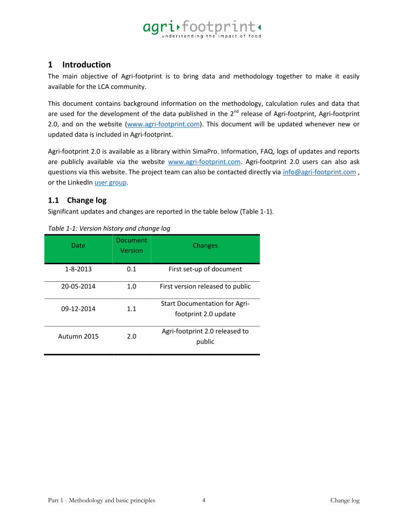
1.1 Change log

Significant updates and changes are reported in the table below (Table 1-1).

Table 1-1: Version history and change log

Date Document

Version Changes

1-8-2013 0.1 First set-up of document

20-05-2014 1.0 First version released to public

09-12-2014 1.1 Start Documentation for Agri-

footprint 2.0 update

Autumn 2015 2.0 Agri-footprint 2.0 released to

public

Part 1 - Methodology and basic principles 5 Project team

1.2 Project team

The development of Agri-footprint was executed by Blonk Consultants. The development team

consisted out of the following members:

Agri-footprint 1.0 (2013-2014):

1. Jasper Scholten

2. Bart Durlinger

3. Marcelo Tyszler

4. Roline Broekema

5. Willem-Jan van Zeist

6. Hans Blonk

Agri-footprint 2.0 (2014-2015):

1. Jasper Scholten

2. Bart Durlinger

3. Roline Broekema

4. Lody Kuling

5. Elsa Valencia-Martinez

6. Laura Batlle Bayer

Blonk Consultants can be contacted through www.blonkconsultants.nl or via LinkedIn. There is also an

Agri-footprint user group on LinkedIn.

Project partners 1.2.1

There was not a specific commissioner of Agri-footprint, however a number of parties have been

involved in sponsoring the development either financially or by delivering data.

Development support and implementation in SimaPro:

PRé Sustainability: www.pre-sustainability.com

Provision of data:

Suiker Unie: www.suikerunie.nl

OCI Nitrogen: www.ocinitrogen.com

Meatless: www.meatless.nl/en

Part 1 - Methodology and basic principles 6 Life Cycle Assessment (LCA) framework

1.3 Life Cycle Assessment (LCA) framework

Life cycle assessment (LCA) is a methodological framework for assessing the environmental impacts that

can be related to the life cycle of a product or service. Examples of environmental impacts are climate

change, toxicological stress on human health and ecosystems, depletion of resources, water use, and

land use.

Historically, most LCAs had a strong focus on consumer goods originating from industrial processes, such

as packaging, diapers, plastic and metal goods. LCAs on agricultural goods were performed less often

and methodology development on LCA of agricultural products received also less attention. During the

1990s, some publications on methodology for LCAs of agricultural products appeared (Wegener

Sleeswijk, et al. 1996; Blonk et al., 1997; Audsley et al., 1997).

Nowadays there are several LCA protocols, such as the ISO standards and guidelines for practitioners

that give directions on how to conduct an LCA. Important LCA standards and handbooks that were used

as a basis for the LCIs in Agri-footprint are:

The ISO 14040/44 series (ISO, 2006a, 2006b)

The ILCD handbook (JRC-IES, 2010)

The ISO 14040 series (ISO, 2006a) describe the basic requirements for performing an LCA study. This

includes, amongst others, directions on how to define the functional unit of a product, how to

determine which processes need to be included or excluded, and how to deal with co-production

situations where elementary flows need to be allocated to the different products. However, the ISO

standard can still lead to different methodological decisions, depending on the LCA practitioner’s

interpretation. This means that applying the ISO standards properly may still result in different

approaches and different quantitative results.

For applying ISO standards as properly and as unambiguously as possible, further guidelines on

interpretation are needed. The ILCD handbook (JRC-IES, 2010) gives these guidelines on a practical level.

One of the most valuable methodological additions in the ILCD handbook is the division between

consequential and attributional LCA, which is not made in the ISO standard. The data provided by Agri-

footprint are primarily meant to support attributional LCA studies.

Part 1 - Methodology and basic principles 7 Life Cycle Assessment (LCA) framework

Methodological challenges in agricultural LCAs 1.3.1

Performing LCAs of agriculture production systems introduces some specific topics that hardly prevail in

LCAs of non-agricultural products. It concerns the following generic inventory and impact modelling

issues:

The definition of the system boundary between nature and the economy (for example: Is

agricultural soil part of the economic or the environmental system? How should be dealt with

the emissions of living organisms?).

Some environmental impacts that are specifically important for agriculture are still under

development (for example: soil erosion and soil degradation, water depletion, biodiversity loss

due to land use and land use change or depletion of (fish) stocks).

There is a large heterogeneity in time and place of cultivation induced emissions, depending on

various local conditions

The limited data availability for modelling toxicity impacts.

Relation between soil emissions and differences in climate and soil types (e.g. peat, sand).

Next to these issues, LCAs of agricultural products have to cope with specific allocation issues not

existing elsewhere:

Segregation between animal and plant production systems (e.g. allocation of manure

emissions).

Rotation schemes and fallow land (how to allocate share benefits and emissions to a single crop

in crop rotation schemes).

Methodological guidelines for agricultural LCAs 1.3.2

Wegener Sleeswijk et al (1996) published the first set of guidelines on methodological topics for LCAs of

agricultural products in the Netherlands. As the same need for agricultural specifications was also felt in

other European countries, a number of European research institutes took concerted action to draw up

an harmonised approach for use by European agricultural LCA practitioners (Audsley & Alber, 1997). A

specific PAS 2050 guidance for horticultural products is developed in 2012 (BSI, 2012) and in 2013 the

Environmental Assessment of Food and Drink Protocol (ENVIFOOD) was published by the European Food

Sustainable Consumption and Production Round Table (Food SCP, 2012).

In the coming years, many food related LCAs will be performed due to the special attention from the

European Commission for food, feed and beverages in the Product Environmental Footprint (PEF)

program. Also the European research and innovation programme Horizon 2020 focuses on more

sustainable food production systems which have to include a LCA in line with the ILCD handbooks. A

recently methodological development is Livestock Environmental Assessment and Performance

Partnership (LEAP, coordinated by FAO). LEAP publishes sector specific LCA guidelines for livestock

production systems and feed. This document and the database are drafted as much as possible in line

with the guidelines from the ILCD handbook “Specific guide for Life Cycle Inventory data sets” (JRC-IES,

2010). The treatment of methodological issues such as allocation, naming conventions and modelling

principles will be discussed in this document.

Part 1 - Methodology and basic principles 8 Reasons for development

2 Goal

2.1 Reasons for development The main reason for development of Agri-footprint is the database developer perspective (JRC-IES,

2010); to develop descriptive high-quality generic LCI data on a range of products. These LCI data can

subsequently be used for a multitude of LCAs. By having these generic LCIs readily available, future LCAs

can be developed more efficiently. Also, some company specific life cycle inventories are included in

Agri-footprint (currently Nutramon fertilizer from OCI, sugar products from Suiker Unie and Meatless

which are vegetable fat free fibres). By making the better performance of specific companies visible, LCA

users can more easily identify improvement options in a lifecycle.

The target audiences are LCA practitioners and environmental specialists in the agricultural, food

production, environmental and related sectors. Agri-footprint is intended to be used in the public

domain and is available to LCA and sustainability experts that have a SimaPro license. It is expected that

this audience has at least a basic understanding of life cycle concepts.

2.2 Intended applications Agri-footprint aims to support both type A (“Micro level decision support”) and C (“Accounting”)

applications, including interactions with other systems (C1) as well as isolated systems (C2), as described

in the ILCD guidelines (JRC-IES, 2010). Agri-footprint is based on an attributional approach. This means

that the results give an impression of the environmental impact of a product in the current situation.

Agri-footprint does not aim to support type B (“Meso/macro-level decision support”), where LCI

modelling exclusively refers to those processes that are affected by large-scale consequences. The

processes in Agri-footprint are not modelled in a consequential way.

Agri-footprint can be used as a secondary data source to support comparisons or comparative assertions

across systems (e.g. products). It is the responsibility of the practitioner to ensure ISO

14040:2006/14044:2006 compliance (through an ISO review of the study), in case a LCA should be used

to make public claims. This document provides all relevant information to facilitate this process, through

transparent documentation of methodological choices and through description of data sources and

modelling. Ref to Part 2 report. In some comparative LCA cases, a consequential approach may be more

appropriate. In that case, the user may need to modify the LCIs to accurately reflect marginal effects.

More specifically, potential applications of Agri-footprint may be:

The identification of key environmental performance indicators of a product group

Hotspot analysis of a specific agricultural product.

Benchmarking of specific products against a product group average.

To provide policy information by basket-of-product type studies or identifying product groups

with the largest environmental impact in a certain context.

Part 1 - Methodology and basic principles 9 Intended applications

Agri-footprint also supports other applications; however additional modelling (or modification of

datasets) will be required:

Strategic decision making by providing the possibility of forecasting and analysis of the

environmental impact of raw material strategies and identifying product groups or raw

materials with the largest environmental improvement potential.

Agri-footprint supports detailed product design of food products, in which the data from Agri-

footprint can be used as a starting point.

Agri-footprint also supports the development of life cycle based Eco label criteria, but does not

provide Eco label criteria directly.

Agri-footprint can be referred to as a prescribed secondary data source to be used in life cycle

based environmental declarations of specific (food) products under the Product Environmental

Footprint (PEF) framework, or in Product Category Rules (PCRs).

Agri-footprint is not intended to be used for:

Green public or private procurement, as Agri-footprint does not (yet) provide sufficient data on

supplier or brand specific products (although this may change in the future, as incorporation of

supplier specific data is desired).

Agri-footprint is not intended for corporate or site specific environmental reporting or

environmental certification of specific life cycles, although Agri-footprint may be used as a

source for background data.

Agri-footprint provides LCI datasets on unit process level with fixed values. Agri-footprint unit processes

are linked so that detailed, interconnected, LCI models can be applied directly as input into LCAs. Agri-

footprint uses some background data that was sourced from ELCD datasets (JRC-IES, 2012). A list of

these used ELCD processes is provided in the data report (Agri-footprint 2.0 - Part 2 – Description of

data).

Part 1 - Methodology and basic principles 10 Definition of included processes

3 Scope

3.1 Definition of included processes Agri-footprint contains LCIs of food and feed products and their intermediates. These unit processes are

linked in Agri-footprint to produce commonly used food commodities. The system boundaries are from

cradle to factory gate (as shown in the figures of section 3.5). Retail, preparation at the consumer and

waste treatment after use are not incorporated in Agri-footprint. (Consumer) packaging is generally not

included in Agri-footprint.

The processes in Agri-footprint reflect an average performance for a defined region for a certain period

of time, for instance wheat cultivation in the Netherlands, or crushing of soy beans in the United States.

The data description section of the report (“Agri-footprint 2.0 - Part 2 – Description of data”) gives more

detail on how the data is generated.

3.2 Consistency of methods, assumptions and data The data in Agri-footprint are derived from different sources. The LCIs for the animal production

systems, transport, auxiliary materials, fertilizers etc. have been developed based on previous public

studies of Blonk Consultants. In these studies, data were collected mainly from the public domain

(scientific literature, FAOstat, Eurostat, etc.) or from public or confidential research initiated by the

industry and conducted by Blonk Consultants. Where possible, the data have been reviewed by industry

experts. Data gaps were filled with estimates, which were as much as possible based on industry expert

opinions. The assumptions are documented in this report, and clearly identified in the database.

3.3 Function, functional unit and reference flow In the appendix of in ‘Agri-footprint 2.0 - Part 2 – Description of data’, a list of all products in Agri-

footprint is provided. Products can fulfill different functions, which depend on the context in which they

are used. It is therefore not possible to define a complete functional unit for every product in the

database. Rather, reference flows can be defined, that can fulfill different functions in different

contexts. To allow for maximum modelling flexibility, a number of properties of the reference flow are

provided in the database. For example, the main reference flow for crop cultivation is 1 kg of crop, but

the dry matter and energy content are given as additional properties. The general principle used in Agri-

footprint is that the reference flows of products reflect ‘physical’ flows as accurately as possible, i.e.

reference flows are expressed in kg product “as traded”; thus including moisture, formulation agents

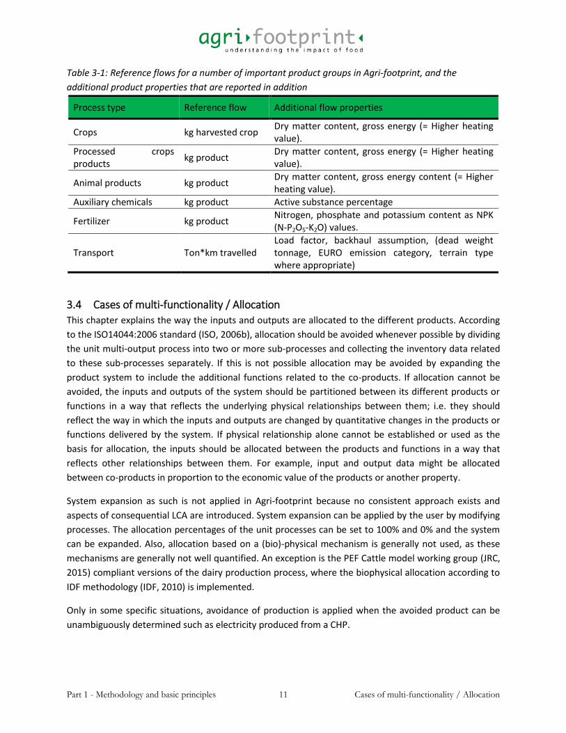
etc., with product properties listed separately in the process name and/or comment fields. Table 3-1

lists the reference flows for a number of important product groups in Agri-footprint, and the additional

flow properties that are reported in addition. These additional properties may be used to construct

alternative reference flows.

Part 1 - Methodology and basic principles 11 Cases of multi-functionality / Allocation

Table 3-1: Reference flows for a number of important product groups in Agri-footprint, and the

additional product properties that are reported in addition

Process type Reference flow Additional flow properties

Crops kg harvested crop Dry matter content, gross energy (= Higher heating value).

Processed crops products

kg product Dry matter content, gross energy (= Higher heating value).

Animal products kg product Dry matter content, gross energy content (= Higher heating value).

Auxiliary chemicals kg product Active substance percentage

Fertilizer kg product Nitrogen, phosphate and potassium content as NPK (N-P2O5-K2O) values.

Transport Ton*km travelled Load factor, backhaul assumption, (dead weight tonnage, EURO emission category, terrain type where appropriate)

3.4 Cases of multi-functionality / Allocation This chapter explains the way the inputs and outputs are allocated to the different products. According

to the ISO14044:2006 standard (ISO, 2006b), allocation should be avoided whenever possible by dividing

the unit multi-output process into two or more sub-processes and collecting the inventory data related

to these sub-processes separately. If this is not possible allocation may be avoided by expanding the

product system to include the additional functions related to the co-products. If allocation cannot be

avoided, the inputs and outputs of the system should be partitioned between its different products or

functions in a way that reflects the underlying physical relationships between them; i.e. they should

reflect the way in which the inputs and outputs are changed by quantitative changes in the products or

functions delivered by the system. If physical relationship alone cannot be established or used as the

basis for allocation, the inputs should be allocated between the products and functions in a way that

reflects other relationships between them. For example, input and output data might be allocated

between co-products in proportion to the economic value of the products or another property.

System expansion as such is not applied in Agri-footprint because no consistent approach exists and

aspects of consequential LCA are introduced. System expansion can be applied by the user by modifying

processes. The allocation percentages of the unit processes can be set to 100% and 0% and the system

can be expanded. Also, allocation based on a (bio)-physical mechanism is generally not used, as these

mechanisms are generally not well quantified. An exception is the PEF Cattle model working group (JRC,

2015) compliant versions of the dairy production process, where the biophysical allocation according to

IDF methodology (IDF, 2010) is implemented.

Only in some specific situations, avoidance of production is applied when the avoided product can be

unambiguously determined such as electricity produced from a CHP.

Part 1 - Methodology and basic principles 12 Cases of multi-functionality / Allocation

It should also be realised that allocation on the basis of physical keys of the outputs is not the same as

allocation on the basis of (bio) physical mechanism, but could be considered a proxy for this approach.

Likewise, economic allocation may be regarded as a proxy for a market based approach (substitution

through system expansion). If allocation keys are not directly related to a physical mechanism, they

should be treated as allocation on the basis of another causality (ISO step 3). Therefore all three

allocation types in Agri-footprint should be regarded as ‘allocation based on another causality’.

Allocation types applied in Agri-footprint 3.4.1

Agri-footprint currently contains three types of allocation, mass allocation, energy allocation and

economic allocation.

1. Mass allocation: For the crops and the processing of the crops, mass allocation is based on the

mass of the dry matter of the products. For the animal products, mass allocation is based on the

mass as traded.

2. Gross energy allocation: Water has a gross energy of 0 MJ/kg. The gross energy for protein, fat

and carbohydrates are respectively: 23.6, 39.3 and 17.4 MJ/kg which are based on USDA (1973).

Nutritional properties for gross energy calculations of products are based on a nutritional feed

material list (Centraal veevoederbureau, 2010). For the other products, the references to the

gross energy are given in the chapters on these products in in ‘Agri-footprint 2.0 - Part 2 –

Description of data’.

3. Economic allocation: For the crops and the processing of the crops the economic value of the

products is based on Vellinga et al. (2013). For the other products, the references to the

economic value are given in the chapters on these products in ‘Agri-footprint 2.0 - Part 2 –

Description of data’.

Allocation is applied without the use of cut-offs for so called residual product streams whenever

possible. There are three exceptions to this allocation rule:

Citrus pulp dried, from drying, at plant

Brewer's grains, wet, at plant

Animal manure

The reason for these exceptions is pragmatism. These products are required for the LCI of a couple of

animal production systems and were derived from the Feedprint database where the upstream

processes were not modelled because of the application of the residual principle. This may be adapted

in a future update of Agri-footprint. Dried citrus pulp and wet brewer’s grain do not include any inputs

from previous life cycle stages. Dried citrus pulp only includes the energy required for drying.

Animal manure is considered to be a residual product of the animal production systems and does not

receive part of the emissions of the animal production system1 when animal manure is applied.

1 The animal production systems are single farming systems and not mixed farming systems.

Part 1 - Methodology and basic principles 13 System boundaries

3.5 System boundaries

Agri-footprint covers potential impacts on the three areas of protection (Human Health, Natural

Environment and Natural Resources) that are caused by interventions between technosphere and

ecosphere that occur during normal operation (thus excluding accidents, spills and other unforeseeable

incidents).

The LCI data is ‘cradle-to-gate’, where the gate is dependent on the process analysed. No data on

distribution to retail, retail, consumer use and end of life (after the use phase) are provided (but

treatment of waste generated during processing is included). All processes that are relevant for analysis

on an attributional basis are included. Any omission or deviation is documented in the documentation of

the specific process.

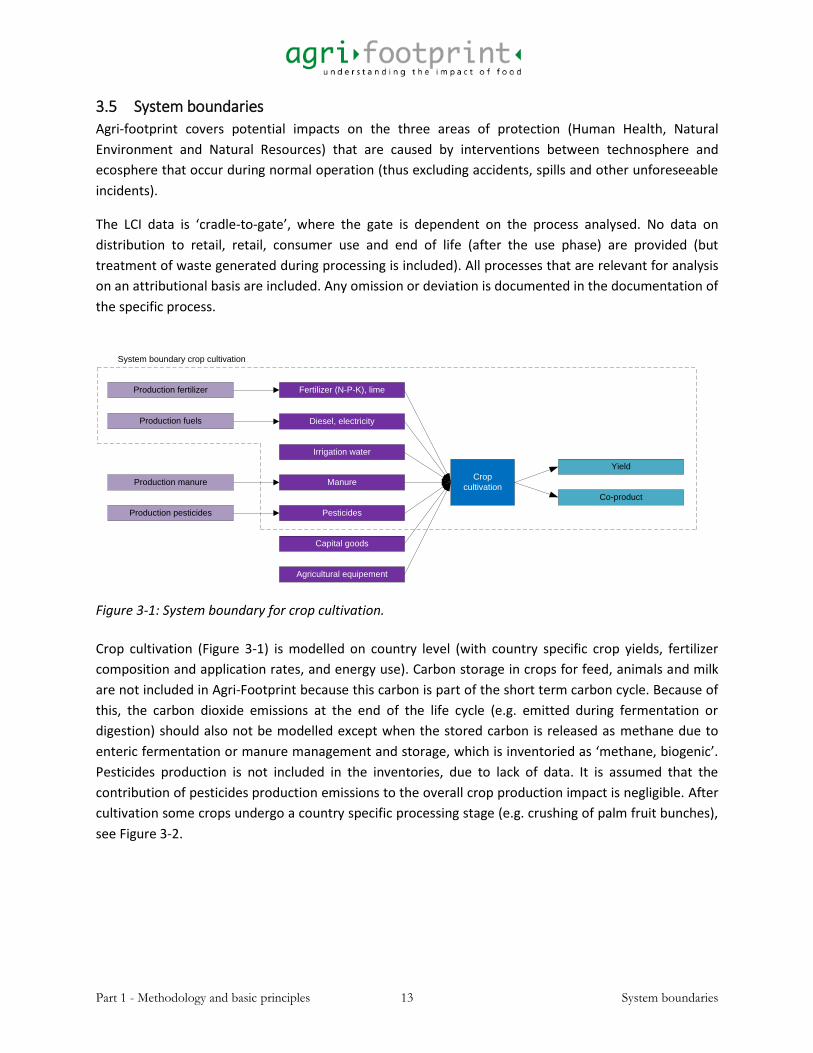
Figure 3-1: System boundary for crop cultivation.

Crop cultivation (Figure 3-1) is modelled on country level (with country specific crop yields, fertilizer

composition and application rates, and energy use). Carbon storage in crops for feed, animals and milk

are not included in Agri-Footprint because this carbon is part of the short term carbon cycle. Because of

this, the carbon dioxide emissions at the end of the life cycle (e.g. emitted during fermentation or

digestion) should also not be modelled except when the stored carbon is released as methane due to

enteric fermentation or manure management and storage, which is inventoried as ‘methane, biogenic’.

Pesticides production is not included in the inventories, due to lack of data. It is assumed that the

contribution of pesticides production emissions to the overall crop production impact is negligible. After

cultivation some crops undergo a country specific processing stage (e.g. crushing of palm fruit bunches),

see Figure 3-2.

Crop

cultivation

Fertilizer (N-P-K), lime

Irrigation water

Manure

Diesel, electricity

Pesticides

Production fertilizer

Production fuels

Production manure

Production pesticides

Capital goods

Agricultural equipement

Yield

Co-product

System boundary crop cultivation

Part 1 - Methodology and basic principles 14 System boundaries

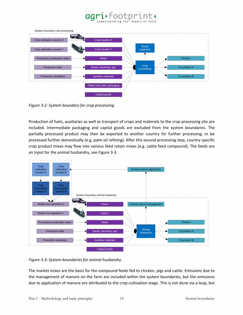
Figure 3-2: System boundary for crop processing.

Production of fuels, auxiliaries as well as transport of crops and materials to the crop processing site are

included. Intermediate packaging and capital goods are excluded from the system boundaries. The

partially processed product may then be exported to another country for further processing, or be

processed further domestically (e.g. palm oil refining). After this second processing step, country specific

crop product mixes may flow into various feed ration mixes (e.g. cattle feed compound). The feeds are

an input for the animal husbandry, see Figure 3-3.

Figure 3-3: System boundaries for animal husbandry.

The market mixes are the basis for the compound feeds fed to chicken, pigs and cattle. Emissions due to

the management of manure on the farm are included within the system boundaries, but the emissions

due to application of manure are attributed to the crop cultivation stage. This is not done via a loop, but

Crop

processing

Crop country X

Water

Diesel, electricity, gas

Crop country Y

Auxiliary materials

Crop cultivation country X

Crop cultivation country Y

Production fuels

Production auxiliaries

Pallets and other packaging

Capital goods

Product

Co-product A

System boundary crop processing

Production/ purification water

Co-product B

Waste

treatment

Animal

husbandry

Feed I

Water

Diesel, electricity, gas

Feed II

Auxiliary materials

Market mix ingredient X

Market mix ingredient Y

Production fuels

Production auxiliaries

Capital goods

Product

Co-product A

System boundary animal husbandry

Production/ purification water

Co-product B

Crop

processing

country A

Crop

processing

country B

Crop

cultivation

country A

Crop

cultivation

country B

Animal manure management

Animal manure application

Part 1 - Methodology and basic principles 15 System boundaries

when a crop is cultivated using manure this is modelled within the crop cultivation itself, not taking into

account any emissions from the animal husbandry. So the manure is treated via a cut-off. Emissions due

to animal manure transport to the field are 100% allocated to crop cultivation.

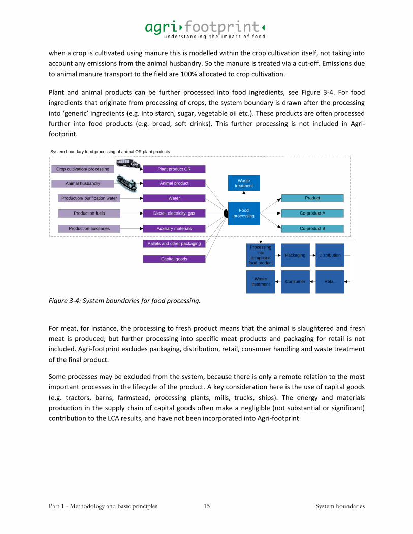
Plant and animal products can be further processed into food ingredients, see Figure 3-4. For food

ingredients that originate from processing of crops, the system boundary is drawn after the processing

into ‘generic’ ingredients (e.g. into starch, sugar, vegetable oil etc.). These products are often processed

further into food products (e.g. bread, soft drinks). This further processing is not included in Agri-

footprint.

Figure 3-4: System boundaries for food processing.

For meat, for instance, the processing to fresh product means that the animal is slaughtered and fresh

meat is produced, but further processing into specific meat products and packaging for retail is not

included. Agri-footprint excludes packaging, distribution, retail, consumer handling and waste treatment

of the final product.

Some processes may be excluded from the system, because there is only a remote relation to the most

important processes in the lifecycle of the product. A key consideration here is the use of capital goods

(e.g. tractors, barns, farmstead, processing plants, mills, trucks, ships). The energy and materials

production in the supply chain of capital goods often make a negligible (not substantial or significant)

contribution to the LCA results, and have not been incorporated into Agri-footprint.

Food

processing

Water

Diesel, electricity, gas

Animal product

Auxiliary materials

Animal husbandry

Production fuels

Production auxiliaries

Pallets and other packaging

Capital goods

Product

Co-product A

System boundary food processing of animal OR plant products

Production/ purification water

Co-product B

Plant product ORCrop cultivation/ processing

Packaging Distribution

Consumer RetailWaste

treatment

Waste

treatment

Processing

into

composed

food product

Part 1 - Methodology and basic principles 16 Cut-off

3.6 Cut-off

The cut-off criteria for the inclusion of inputs and outputs were based on mass and/or energy

consumption. It is estimated that elementary flows representing not more than 2% of the cumulative

mass and energy flows were omitted.

3.7 Basis for impact assessment

The LCIA methods ReCiPe 1.11 (PRé Consultants, Radboud University Nijmegen, Leiden University, &

RIVM, 2014) and ILCD 1.05 (JRC-IES, 2014) were taken into account when developing Agri-footprint, but

Agri-footprint may also support other impact assessment methods.

In Agri-footprint, climate change due to land use change has been modelled separately in the emissions

to air: Carbon dioxide, land transformation. This makes it possible to report on the effects of land use

change separately. Land use change is also modelled in m2 land transformation in the known inputs

from nature. Although m2 land transformation contributes to other environmental indicators than

carbon dioxide, please keep in mind that double counting of the impact of land use change should be

avoided.

Agri-footprint makes use of other databases like ELCD to provide data for some background processes. If

LCIs of other databases are used, it is possible that errors have occurred during the implementation of

those datasets into third party LCA-software. It remains to the user of Agri-footprint to select the impact

categories that are environmentally relevant for the analysed products or systems and to check which

impact categories are endorsed by other bodies of the relevant region. The inventories in Agri-footprint

support the calculation of the midpoint impact categories being proposed in the EU PEF (Product

Environmental Footprint) and ENVIFOOD protocol.

Part 1 - Methodology and basic principles 17 Treatment of uncertainty

3.8 Treatment of uncertainty

Uncertainty in inventory data exists in many ways and there are many factors determining the level of

uncertainty in LCA (Huijbregts et al., 2001). The majority of the inventory data in Agri-footprint are not

the result of actual measurements but of models that compute inventory data in relation to activity data

that are on its turn measured or estimated. We use the following classification derived from … to explain

the different types of uncertainties and how we have treated and estimated uncertainties:

1. Uncertainty due to LC modelling choices which are related to the simplifications made in

modelling the lifecycles, for instance by using cut off rules for marginal inputs and outputs or

excluding not common situations in defining the average lifecycle;

2. Data uncertainty which encompasses inaccuracy of data and lack of (representative) data;

3. Emission model and parameter uncertainty which refers to the many emissions which are

calculated by combining primary activity data with an emission factor that is the result of a

parameterized model;

4. Spatial variability refers to the variation in conditions (soil, climate) and applied technologies

(age, type, abatement techniques, etc.) the region under study

5. Temporal variability refers to variation in time related to variation in natural conditions over the

years (climate, pests, capacity usage, calamities, et cetera).

Which uncertainty types are included and how 3.8.1

In Agri-footprint, uncertainty distributions are defined for specific input or output data of LCI processes

that incorporate some main factors defining uncertainty and variability around the average. There we

focus on key parameters related to the average efficiency of processes in the regions for which average

process data are derived. This overall distribution combines the variability in technology, processing

conditions and management, which may have a spatial correlation in that region (see Table 3-2 for

further explanation).

Part 1 - Methodology and basic principles 18 Treatment of uncertainty

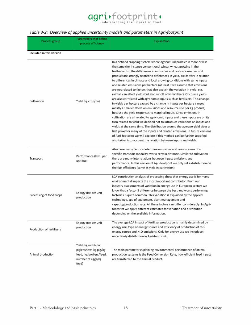
Table 3-2: Overview of applied uncertainty models and parameters in Agri-footprint

Process group Parameters that define

process efficiency Explanation

Included in this version

Cultivation Yield (kg crop/ha)

In a defined cropping system where agricultural practice is more or less

the same (for instance conventional winter wheat growing in the

Netherlands), the differences in emissions and resource use per unit

product are strongly related to differences in yield. Yields vary in relation

to differences in climate and local growing conditions with same inputs

and related emissions per hectare (at least if we assume that emissions

are not related to factors that also explain the variation in yield, e.g.

rainfall can effect yields but also runoff of N-fertilizer). Of course yields

are also correlated with agronomic inputs such as fertilizers. This change

in yields per hectare caused by a change in inputs per hectare causes

mostly a smaller effect on emissions and resource use per kg product,

because the yield responses to marginal inputs. Since emissions in

cultivation are all related to agronomic inputs and these inputs are on its

turn related to yield we decided not to introduce variations on inputs and

yields at the same time. The distribution around the average yield gives a

first proxy for many of the inputs and related emissions. In future versions

of Agri-footprint we will explore if this method can be further specified

also taking into account the relation between inputs and yields.

Transport Performance (tkm) per

unit fuel

Also here many factors determine emissions and resource use of a

specific transport modality over a certain distance. Similar to cultivation

there are many interrelations between inputs emissions and

performance. In this version of Agri-footprint we only set a distribution on

the fuel efficiency (same as yield in cultivation).

Processing of food crops Energy use per unit

production

LCA contribution analysis of processing show that energy use is for many

environmental impacts the most important contributor. From our

industry assessments of variation in energy use in European sectors we

know that a factor 2 difference between the best and worst performing

factories is quite common. This variation is explained by the applied

technology, age of equipment, plant management and

capacity/production rate. All these factors can differ considerably. In Agri-

footprint we apply different estimates for variation and distribution

depending on the available information.

Production of fertilizers

Energy use per unit

production

The average LCA impact of fertilizer production is mainly determined by

energy use, type of energy source and efficiency of production of this

energy source and N2O emissions. Only for energy use we include an

uncertainty distribution in Agri-footprint.

Animal production

Yield (kg milk/cow;

piglets/sow; kg pig/kg

feed; kg broilers/feed,

number of eggs/kg

feed)

The main parameter explaining environmental performance of animal

production systems is the Feed Conversion Rate, how efficient feed inputs

are transferred to the animal product.

Part 1 - Methodology and basic principles 19 Treatment of uncertainty

In Agri-footprint we included not all uncertainties:

1. Uncertainty due to LCA modelling arising when modifications are made in process information

to simplify or generalize the process was neglected. Examples are neglecting small inputs and

outputs of the dairy farm system and assuming that the dairy farm is on average a closed system

or only taking into account a limited set of technologies for housing systems in defining the

average pig farming system.

2. Model uncertainty is especially important for the calculation of N2O, CH4, NH3 to air emissions, N

to water, P to water and agricultural soil, heavy metals to water and soil. The literature that

describes the applied models often gives estimates for uncertainty in the relations between

input and output (e.g. the N2O emission to air due to N-fertilizer application to the soil). These

uncertainties are not included and can be quite high in some specific cases, such as N2O and

NO3. Also the choice for specific emission models is not considered.

3. Not included data uncertainties around the average process are:

3.a. Variation in mass balances of multi-output processes and the variation in the balance of

input products and output products, for instance the yield of wheat flour and wheat

bran that can vary in relation to the composition of the incoming wheat. Secondly, the

variation in composition of product mixes, such as the market mixes, the energy mix,

the mix of transport modality and the mix of feed ingredients in a compound feed.

3.b. Variation in the allocation parameters, energy content and price. Most variable are the

prices, although by using five years averages the variation is not so big (see Blonk &

Ponsioen, 2009). Energy values used for allocation can also slightly vary.

3.c. Uncertainty in emissions that are related to specific techniques, such as ammonia

releases of pig housing systems, emissions of pesticides in relation to spraying

conditions, etc.

Part 1 - Methodology and basic principles 20 Treatment of uncertainty

Overview of applied uncertainty information 3.8.2

In Table 3-3, an overview is given of applied uncertainty models and parameters. Most of these

estimates are based on expert judgements using the following principles regarding distribution and

variation:

If there is only information about the range, for instance from literature describing the

performance of technologies in practices (such as the BREF reports), a triangular distribution is

assumed around the average of this range (min, max, average).

If there is more information available, such as more data on performance and representativeness of

this performance in the total range of practices that define the average,

o A normal or a lognormal distribution is derived using the following rules of thumb:

A normal distribution is assumed for farming (cultivation and animal farming).

A lognormal distribution is assumed for all other processes.

o To determine the size of the distribution:

If specific information is available of the distribution and standard deviation of the

average process, then this is applied.

If there is no specific information available, information is derived from other processes

that are similar based on expert judgment using the following information:

In processing industry, the distance between the best and worst performing

industry in a region lays in general between a factor 2 to 3. The higher the share

of energy costs in the total costs of an industry the smaller the distribution.

In non-land based animal production systems (broilers, pigs and egg production)

there is a very big pressure on having a good feed conversion rate (FCR). So the

distributions around the FCR are small.

In land based farming, the cost breakdown and also natural conditions are more

defining variability, so there is a wider distribution around the average.

Part 1 - Methodology and basic principles 21 Treatment of uncertainty

Table 3-3: Overview of applied uncertainty models and parameters

Process Data point Uncertainty model and parameters Source

Cultivation

Kg crop production (main + co-products)/ha

Normal distribution, standard deviation is derived from statistical analysis of FAO yield data of the years 2006-2013.

FAOstat (FAO, 2012)

Transport Tonne*km Lognormal distribution, sd = 1.3 Qualified estimate based on sample of primary data of truck fuel consumption and expert judgement

Processing of food crops

Energy use

Mostly Lognormal distributions with a standard deviation varying from 1.1 to 1.4 Sometimes triangular or uniform distributions based on min and max values.

Expert judgement as applied in Feedprint documentation

Production of fertilizer

Energy use

Energy use for ammonia production has a lognormal distribution with sd of 1.35. This value is applied to all fertilizer production energy inputs.

(International Fertilizer Industry Association, 2009)

Animal production

Dairy farm

Normal distribution, coefficient of variation 0.144 of average for the outputs (milk, calves and slaughter cows) as a group.

Based on inventory of a sample of 100 something farmers of a Dutch co-operation (Kramer, Broekema, Tyszler, Durlinger, & Blonk, 2013)

Piglet farm

Outputs piglet and slaughter sows: Normally distributed. Coefficient of variation 0.077

Based on Agrovision benchmark reporting (Agrovision, 2013)

Pig farm

Outputs fattening pigs: Normally distributed. Coefficient of variation 0.061

Based on Agrovision benchmark reporting (Agrovision, 2013)

Raising laying hens

Output laying hens: Normally distributed. Coefficient of variation 0.03

Based on uncertainties around FCR (Wageningen UR, 2013)

Egg production Outputs eggs: Normally distributed. Coefficient of variation 0.06

Same value taken as for Pigs and broiler parent hens, assuming that margins are similar tight and that FCR is key to realize margins

Broiler parent hens

Outputs broiler parent hens: Normally distributed. Coefficient of variation 0.06

Based on uncertainties around FCR (Wageningen UR, 2013)

Broilers

Output: broiler; Normally distributed. Coefficient of variation 0.05

Based on uncertainties FCR. Leinonen, Williams, Wiseman, Guy, & Kyriazakis (2012) gives an estimate between 0.3 and 0.5

Irish beef Outputs: Normally distributed. Coefficient of variation 0.144

Derived from Dutch dairy farming

Part 1 - Methodology and basic principles 22 Treatment of uncertainty

Technical note on the modelling of output uncertainties 3.8.3

SimaPro, does not allow for a direct definition of a probability distribution of outputs. This is solved by

defining a parameter with a probability distribution and use this parameter as the value of the output,

when only one output is defined for a process.

For the multi-output processes a similar strategy was used. We do not include variation in the relative

mass balances of the multiple outputs nor the variation on the allocation factors. Thus it is assumed that

the ratios among the multiple outputs are constant. To keep the ratio between outputs constant (during

an uncertainty analysis) one of the multiple outputs is selected to describe the variability of the process

(reference output). A parameter with the corresponding probability distribution is created for the

reference output. For each additional output, two parameters are created: a parameter which describes

the constant ratio between the additional output and the reference output and a calculated parameter

which multiplies the reference output value by the constant ratio. This construction allows for variation

of the outputs during Monte Carlo analyses, while keeping the ratio between the outputs fixed.

Part 1 - Methodology and basic principles 23 Treatment of uncertainty

4 Data quality procedure To ensure a database with consistent data, a four stage data quality procedure has been used. Each

stage of the procedure focusses on different aspects, to ensure an efficient but at the same time robust

work procedure. Each step of the procedure has been done by a different researcher.

Figure 4-1: Data quality procedure

Part 1 - Methodology and basic principles 24 Selection data sources

4.1 Selection data sources

During the development of Agri-footprint, the following procedure was used to develop the inventories:

1. Establish a consistent baseline dataset

2. Fill data gaps with best available data

3. Improve baseline data whenever possible using data quality hierarchy

Table 4-1: Applied Data quality hierarchy

Data collection method Geography Time Completeness Technology

Most

preferred

Data from all companies

Specified

geographic

region

A year within

the last 5

years

All relevant input

and output flows

Almost all of

the common

technologies

Sample of companies made

on target LCI data

performance

Verified/non verified

Sample of companies based

on other performance (e.g,

economic)

Verified/non verified Similar

geographic

region

Different

years within

the last 10

years

Some major flows

are missing

A commonly

used

technology

Documented expert data

describing technology inputs

and environmental

performance

Statistical data having a

broader scope

Anecdotal data from other

sources Geographic

region

dissimilar

More than 10

years

Many major flows

are missing

An alternative

technology Least

preferred

Assumptions, proxies using

analogous processes, partial

modelling

Establish a consistent baseline dataset as a starting point 4.1.1

During the development of Agri-footprint, the first step was to create data that was of consistent quality

for all crops and regions covered. For example, all fertilizer application rates, fertilizer types, water use

etc. is based on the same methodologies for all crops. To create this consistent baseline dataset, data

were derived from documented expert data or data from statistics (i.e. data source in the middle of the

data hierarchy).

Part 1 - Methodology and basic principles 25 Selection data sources

Agri-footprint contains attributional LCIs, so generally average mixes are considered that are

representative for the specific crop, process, transport modality, product or location.

The main baseline data source is the public domain (Scientific literature, FAOstat, Eurostat, etc.). Data

from the public domain are assessed based on representativeness (time-related coverage, technical

coverage and geographical coverage), completeness, consistency and reproducibility. When data from

public or confidential research initiated by the industry and conducted by Blonk Consultants are more

representative, complete or consistent, these data were used. Where possible, the data have been

reviewed by industry experts.

Fertilizers production was modeled based on the latest available literature and the modeling of a

specific fertilizer product was based on primary data from a large Dutch fertilizer producer (Calcium

Ammonium Nitrate produced by OCI Nitrogen in the Netherlands). Auxiliary materials were based on

the ELCD 3.0 database or literature sources. For some background processes, estimates had to be made

(e.g. the production of asbestos used in sodium hydroxide production which is used in vegetable oil

refining), and these processes are of lower quality and representativeness.

Processing inventories were initially drawn from the feedprint study (Vellinga et al., 2013). These

inventories are generic for all provided countries and regions. These processes are either largely similar

between countries or the data available was not specific enough to create country/ region specific

processes. These generic processes are regionalised by adapting the inputs for energy consumption to

the country or region where the processing takes place. This means that the processing (mass balances,

inputs etc.) is the same for all regions. Therefore that the representativeness may have decreased for

these processes (as the geography of the data is “other region assumed similar”). During the

development of Agri-footprint 2.0, some of these ‘feedprint’ processes have been replaced by higher

quality processes using region specific / higher quality data (see Part 2 of the report).

Transport distances and modes from and to the processing plant are also country specific. The

geographical representativeness will be improved in future upgrades of Agri-footprint.

The aim for the LCI data is to be as recent as possible, which means that when better quality data or

statistics on the processes/ systems are available, these will be incorporated in Agri-footprint, generally

using five year averages. To ensure the best time related representativeness, data will be updated

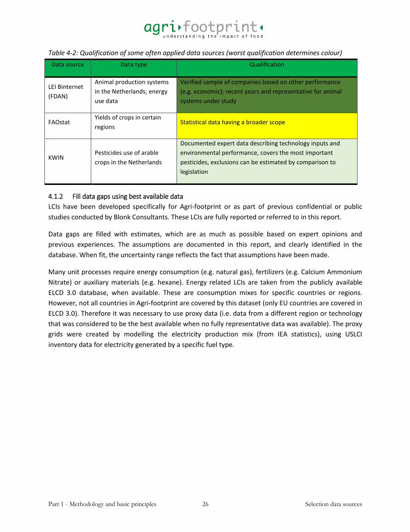
regularly. In Table 4-2, an overview is given of regularly updated data sources in Agri-footprint, and their

place in the data hierarchy.

Part 1 - Methodology and basic principles 26 Selection data sources

Table 4-2: Qualification of some often applied data sources (worst qualification determines colour)

Data source Data type Qualification

LEI Binternet

(FDAN)

Animal production systems

in the Netherlands; energy

use data

Verified sample of companies based on other performance

(e.g. economic); recent years and representative for animal

systems under study

FAOstat Yields of crops in certain

regions Statistical data having a broader scope

KWIN Pesticides use of arable

crops in the Netherlands

Documented expert data describing technology inputs and

environmental performance, covers the most important

pesticides, exclusions can be estimated by comparison to

legislation

Fill data gaps using best available data 4.1.2

LCIs have been developed specifically for Agri-footprint or as part of previous confidential or public

studies conducted by Blonk Consultants. These LCIs are fully reported or referred to in this report.

Data gaps are filled with estimates, which are as much as possible based on expert opinions and

previous experiences. The assumptions are documented in this report, and clearly identified in the

database. When fit, the uncertainty range reflects the fact that assumptions have been made.

Many unit processes require energy consumption (e.g. natural gas), fertilizers (e.g. Calcium Ammonium

Nitrate) or auxiliary materials (e.g. hexane). Energy related LCIs are taken from the publicly available

ELCD 3.0 database, when available. These are consumption mixes for specific countries or regions.

However, not all countries in Agri-footprint are covered by this dataset (only EU countries are covered in

ELCD 3.0). Therefore it was necessary to use proxy data (i.e. data from a different region or technology

that was considered to be the best available when no fully representative data was available). The proxy

grids were created by modelling the electricity production mix (from IEA statistics), using USLCI

inventory data for electricity generated by a specific fuel type.

Part 1 - Methodology and basic principles 27 Data quality checks during modelling

Improve baseline data whenever possible using the data quality hierarchy 4.1.3

The environmental impact of individual companies within an industry sector easily varies a factor 2 and

sometimes much more (Canadian Fertilizer Industry, 2008). Agri-footprint supports the opportunity to

include validated company specific data. The philosophy of this approach is that by making the improved

performance of specific companies visible, LCA users can more easily identify improvement options in a

lifecycle.

4.2 Data quality checks during modelling

As the original data has been compiled in different software programs and data structures, it is

important to check consistency and correctness of all the data during the implementation process (the

migration to a SimaPro database). Quality checking has been done iteratively. (Parts of) the database

were exported to SimaPro, checked, errors or inconsistencies corrected and data gaps identified. When

identified issues were resolved, a new SimaPro export was made, this was again checked. This process

continued until all identified errors and data gaps were resolved. Different methods were used during

the checking process:

Check naming

Remove duplicate processes, or processes that were very similar (e.g. wheat starch slurries with

slightly different starch contents).

Check correct linking

Remove empty processes whenever possible

Check if newly added processes or flows are applied consistently throughout the database.

Mass balances

o Balances; the amount of dry matter going in should be the same as dry matter going out

as product or waste/emission. The total matter ‘as is’ should be balanced as well.

Sometimes it was possible to also calculate balances of substances (e.g. hexane make-

up should be balanced by hexane emissions during crushing).

o Appropriate waste flows

Transport included in all processes

Logical differences between countries (yields, fertilizer application rates, et cetera)

Consistent calculation methodology

Compare results to existing data from other sources.

4.3 Data Quality Assessment using PEF methodology

The internal Data Quality Assessment provides insight into the quality of individual data sets to the users

of Agri-Footprint. This assessment is in accordance with the 6 main indicators of data quality (briefly

described in the below sections) from the ILCD handbook (JRC-IES., 2010). The calculation of the score

for each data quality indicator and the overall data set has been performed in accordance with the PEF

framework (European Commission, 2013), and they can be found in the comment section of each data

set.

Part 1 - Methodology and basic principles 28 Data Quality Assessment using PEF methodology

The assessment procedure was independently done by two researchers. They scored all data quality

indicators from 1 (excellent) to 5 (very poor) in accordance to PEF (European Commission, 2013) . Both

surveys were compared by the absolute difference of scores between the two researchers (Table 2.6). In

the majority of cases (56%), both researchers came to the same score, while only in 2% of the cases the

difference was 3 or higher. To resolve minor differences of 1 or 2, the average value has been used, and

in the case of a difference of 1, the average is rounded upwards (e.g. a score of 2.5 becomes 3). In case

of a major difference of 3 or 4, the particular indicator for that dataset has been revaluated by more in-

depth research.

Table 2-6: Overview of differences in data quality scores.

Absolute

difference % Rules for scoring

0 56 Value

1 30 Average value rounded upwards

2 12 Average value

3 2 Revaluate in-depth

4 0 Revaluate in-depth

Technological Representativeness (TeR) 4.3.1

The Technological Representativeness (TeR) of a data set is defined by the ILCD as “the degree to which

the data set reflects the true population of interest regarding technology, including for included

background data sets, if any.” For Agri-Footprint we operationalized this indicator by defining 3 levels of

technological foreground representativeness and 2 levels of technological background

representativeness. The decision tree for TeR can be found in figure E.1 in appendix E.

Geographical Representativeness (GR) 4.3.2

The Geographical Representativeness (GR) of a data set is defined by the ILCD as “the degree to which

the data set reflects the true population of interest regarding geography, including for included

background data sets, if any.” For Agri-Footprint we operationalized this indicator by defining 5 levels of

geographical foreground representativeness and 2 levels of geographical background

representativeness. The decision tree for GR can be found in figure E.2 in appendix E.

Time-related Representativeness (TiR) 4.3.3

The Time-related Representativeness (TiR) of a data set is defined by the ILCD as “the degree to which

the data set reflects the true population of interest regarding time / age of the data, including for

included background data sets, if any.” For Agri-Footprint we operationalized this indicator by defining 3

levels of time-related foreground representativeness and 3 levels of time-related background

representativeness. The decision tree for TiR can be found in figure E.3 in appendix E.

Part 1 - Methodology and basic principles 29 External review

Completeness (C) 4.3.4

The Completeness of a data set is defined by the ILCD as “the share of (elementary) flows that are

quantitatively included in the inventory. Note that for product and waste flows this needs to be judged

on a system's level.” For Agri-Footprint we operationalized this indicator by defining 3 levels of

foreground completeness and 2 levels of background completeness. The decision tree for C can be

found in figure E.4 in appendix E.

Parameter uncertainty (P) 4.3.5

The Parameter uncertainty (P) of a data set is defined by the ILCD as a “measure of the variability of the

data values for each data expressed (e.g. low variance = high precision). Note that for product and waste

flows this needs to be judged on a system's level.” For Agri-Footprint we operationalized this indicator

by defining 5 levels of uncertainty in accordance with the PEF (European Commission, 2013). The

decision tree for P can be found in figure E.5 in appendix E.

Methodological appropriateness and consistency (M) 4.3.6

The methodological appropriateness and consistency (M) of a data set is measured in accordance to the

PEF methodology (European Commission, 2013), which scales the score on this indicator relative to its

standards concerning: multi-functionality, end of life modeling and system boundaries. Most data sets in

Agri-Footprint are compliant with or all three requirements set by the PEF methodology. Therefore most

datasets (98%) have a score of 2 for this indicator. The decision tree for M can be found in figure E.6 in

appendix E.

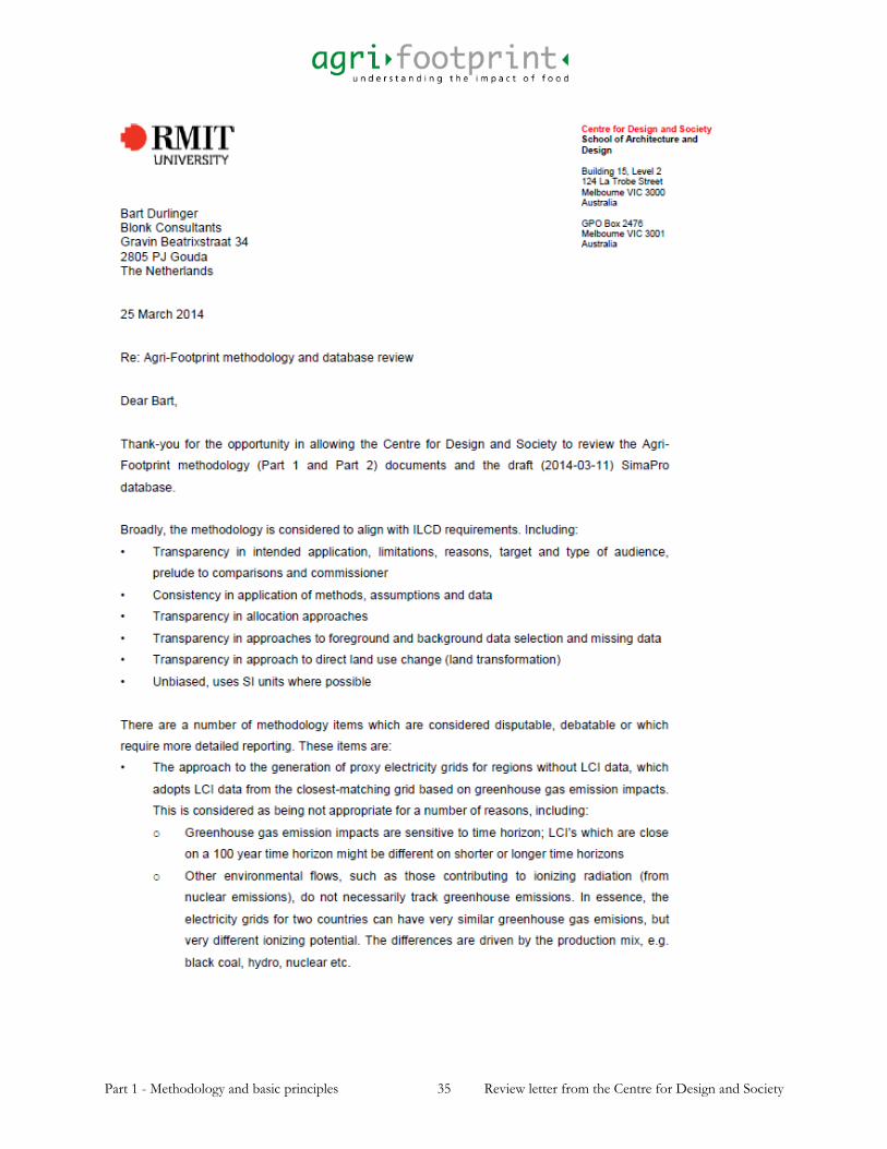
4.4 External review

Agri-footprint 1.0 was externally reviewed on ILCD requirements by the Centre for Design and Society,

RMIT University, Melbourne, Australia. The external reviewers checked the consistency and

transparency of the methodology applied and completeness and transparency of data documentation.

Agri-footprint 2.0 is reviewed by RIVM (Dutch National Institute for Public Health and the Environment).

This critical review is performed to ensure compliance with ISO 14040 (ISO, 2006a), 14044 (ISO, 2006b)

on the following points:

the methods used for the LCIs are consistent with this International Standard,

the methods used for the LCIs are scientifically and technically valid,

the data used are appropriate and reasonable in relation to the, intended goal of the LCIs.

This critical review;

is performed at the end of Agri-footprint 2.0 development,

includes an assessment of the LCI model,

excludes life cycle impact assessment (LCIA).

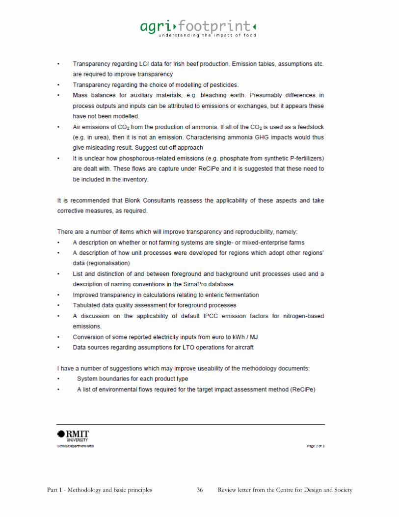
Appendix A contains the original review letter from the Centre for Design (RMIT University). Appendix B

provides responses to the comments and how it is integrated into the final Agri-footprint version.

Appendix C and D contain the review report by RIVM and the response to these comments respectively.

Part 1 - Methodology and basic principles 30 Limitations of Agri-footprint

5 Limitations of Agri-footprint There are a number of limitations that should be taken into account when using Agri-footprint. Some

additional limitations apply to specific processes; these limitations are reported in the data description

section of that specific dataset (in ‘Agri-footprint 2.0 - Part 2 – Description of data’).

Agri-footprint provides LCI data with a standard reference unit of 1 kg. It is the responsibility of the user

to determine an appropriate basis for comparison (functional unit).

The impact categories of ReCiPe and ILCD were taken into account when developing Agri-footprint. Agri-

footprint uses some background data that was sourced from ELCD datasets (JRC-IES, 2012). Where LCIs

of other databases are used, it is possible that errors have occurred during the development of those

datasets or during implementation into third party LCA-software, the correction of these errors are

beyond the control of the Agri-footprint development team. Naturally, errors that were discovered in

those datasets were reported to the appropriate parties.

Elementary flows have been collated to align with requirements of ReCiPe and ILCD. Other LCIA

methods may assess substances which are not included in Agri-footprint.

There are methodological limitations of LCA, which are not specific for Agri-footprint, but which are

relevant for all agricultural and food product life cycle inventories:

There is no internationally accepted methodology which is suitable for use in LCAs for loss of

biodiversity due to land use or direct and indirect land use change.

Multiple methods have been developed internationally on the impact of land use change, but

there is no consensus yet on which method is best. For Agri-footprint the choice was made for

the PAS2050:2012-1 method (BSI, 2012).

For water depletion and water use related to water scarcity there is no international consensus

on the methodology. The water footprint was developed (Hoekstra & et al., 2011) but

internationally there is discussion on whether the green, grey as well as the blue water footprint

are a suitable indicator for environmental impact. Agri-footprint incorporates water use as

regionalized blue water flows to allow impact assessments such as Pfister, Koehler, & Hellweg

(2009) and water resource depletion (Federal Office for the Environment, 2009) as

recommended by the ILCD.

Use of statistical data for crop yields, (artificial and organic) fertilizer application rates, when

there is not specific data available.

Due to limited data availability, elementary flows related to the environmental impact due to

soil erosion and soil degradation is not included in Agri-footprint.

Data availability is also limited in relation to production and the use of pesticides (impacting on

eco-toxicity), but an approach was developed to estimate the impact on ecotoxicity of

agricultural cultivation.

Part 1 - Methodology and basic principles 31 Limitations of Agri-footprint

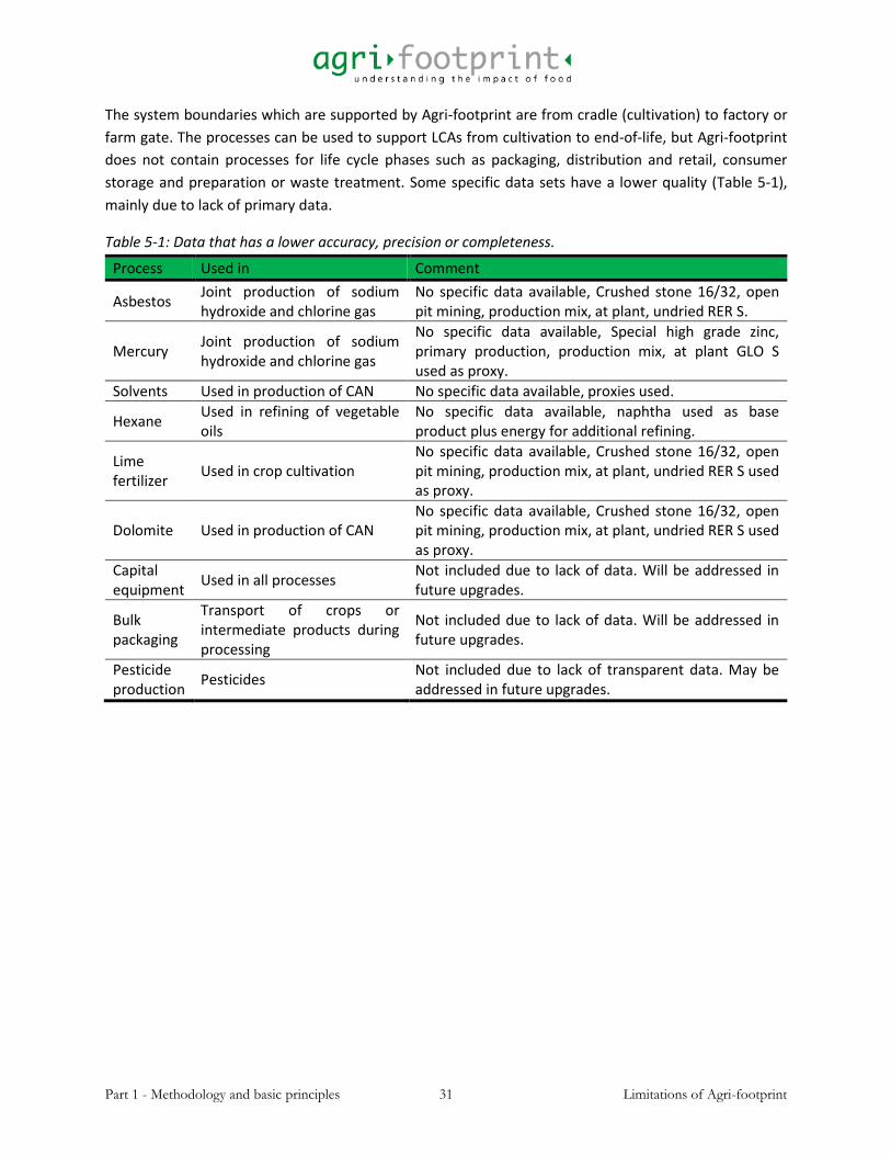
The system boundaries which are supported by Agri-footprint are from cradle (cultivation) to factory or

farm gate. The processes can be used to support LCAs from cultivation to end-of-life, but Agri-footprint

does not contain processes for life cycle phases such as packaging, distribution and retail, consumer

storage and preparation or waste treatment. Some specific data sets have a lower quality (Table 5-1),

mainly due to lack of primary data.

Table 5-1: Data that has a lower accuracy, precision or completeness.

Process Used in Comment

Asbestos Joint production of sodium hydroxide and chlorine gas

No specific data available, Crushed stone 16/32, open pit mining, production mix, at plant, undried RER S.

Mercury Joint production of sodium hydroxide and chlorine gas

No specific data available, Special high grade zinc, primary production, production mix, at plant GLO S used as proxy.

Solvents Used in production of CAN No specific data available, proxies used.

Hexane Used in refining of vegetable oils

No specific data available, naphtha used as base product plus energy for additional refining.

Lime fertilizer

Used in crop cultivation No specific data available, Crushed stone 16/32, open pit mining, production mix, at plant, undried RER S used as proxy.

Dolomite Used in production of CAN No specific data available, Crushed stone 16/32, open pit mining, production mix, at plant, undried RER S used as proxy.

Capital equipment

Used in all processes Not included due to lack of data. Will be addressed in future upgrades.

Bulk packaging

Transport of crops or intermediate products during processing

Not included due to lack of data. Will be addressed in future upgrades.

Pesticide production

Pesticides Not included due to lack of transparent data. May be addressed in future upgrades.

Part 1 - Methodology and basic principles 32 References

6 References

Agrovision. (2013). Kengetallenspiegel.

Audsley, E., & Alber, S. (1997). Harmonisation of environmental life cycle assessment for agriculture. European Comm., DG VI Agriculture.

Blonk, H., & Ponsioen, T. (2009). Towards a tool for assessing carbon footprints of animal feed. Blonk Milieu Advies, Gouda.

BSI. (2012). PAS 2050-1: 2012 Assessment of life cycle greenhouse gas emissions from horticultural products. BSI.

Canadian Fertilizer Industry. (2008). Benchmarking energy efficiency and carbon dioxode emissions.

Centraal veevoederbureau. (2010). Grondstoffenlijst CVB.

European Commission. (2013). COMMISSION RECOMMENDATION of 9 April 2013 on the use of common methods to measure and communicate the life cycle environmental performance of products and organisations. Official Journal of the European Union.

FAO. (2012). Faostat production statistics. Retrieved from http://faostat.fao.org/default.aspx

Federal Office for the Environment. (2009). The Ecological Scarcity Method – Eco-Factors 2006.

Food SCP. (2012). ENVIFOOD Protocol Environmental Assessment of Food and Drink Protocol. Draft Version 0.1.

Hoekstra, A. Y., & et al. (2011). The Water Footprint Assessment Manual. The Water Footprint Network.

Huijbregts, M. A. J., Norris, G., Bretz, R., Ciroth, A., Maurice, B., von Bahr, B., & Weidema, B. (2001). Framework for modelling data uncertainty in life cycle inventories. International Journal of Life Cycle Assessment, 127–132.

IDF. (2010). The IDF guide to standard LCA methodology for the dairy sector. Bulletin of the International Dairy Federation, 445, 1–40.

International Fertilizer Industry Association. (2009). Energy Efficiency and CO2 Emissions in Ammonia Production. Paris.

ISO. (2006a). ISO 14040 Environmental management — Life cycle assessment — Principles and framework.

ISO. (2006b). ISO 14044 - Environmental management — Life cycle assessment — Requirements and guidelines. ISO.

Part 1 - Methodology and basic principles 33 References

JRC. (2015). Baseline Approaches for the Cross-Cutting Issues of the Cattle Related Product Environmental Footprint Pilots in the Context of the Pilot Phase.

JRC-IES. (2010). ILCD handbook - Specific guide for Life Cycle Inventory data sets. doi:10.2788/39726

JRC-IES. (2012). ELCD database. Retrieved from http://elcd.jrc.ec.europa.eu/ELCD3/

JRC-IES. (2014). Characterisation factors of the ILCD Recommended Life Cycle Impact Assessment methods (version 1.05). Retrieved from http://eplca.jrc.ec.europa.eu/?page_id=86

Kramer, G. F. H., Broekema, R., Tyszler, M., Durlinger, B., & Blonk, H. (2013). Comparative LCA of Dutch dairy products and plant- based alternatives. Gouda, the Netherlands.

Leinonen, I., Williams, a G., Wiseman, J., Guy, J., & Kyriazakis, I. (2012). Predicting the environmental impacts of chicken systems in the United Kingdom through a life cycle assessment: broiler production systems. Poultry Science, 91(1), 8–25. doi:10.3382/ps.2011-01634

Pfister, S., Koehler, A., & Hellweg, S. (2009). Assessing the environmental impacts of freshwater consumption in LCA. Environmental Science & Technology, 43(11), 4098–104. Retrieved from http://www.ncbi.nlm.nih.gov/pubmed/19569336

PRé Consultants, Radboud University Nijmegen, Leiden University, & RIVM. (2014). ReCiPe 1.11: Characterisation factors spreadsheet. Retrieved from http://www.lcia-recipe.net/file-cabinet

USDA. (1973). Energy value of foods.

Vellinga, T. V., Blonk, H., Marinussen, M., Zeist, W. J. Van, Boer, I. J. M. De, & Starmans, D. (2013). Report 674 Methodology used in feedprint: a tool quantifying greenhouse gas emissions of feed production and utilization. Retrieved from http://www.wageningenur.nl/nl/show/Feedprint.htm

Wageningen UR. (2013). Kwantitatieve informatie veehouderij 2013-2014. Wageningen UR, Wageningen.

Wegener Sleeswijk, A., Kleijn, R., Van Zeijts, H., Reus, J., Meeusen - van Onna, M., Leneman, H., & Sengers, H. (1996). Application of LCA to agricultural products. Leiden: CML.

Part 1 - Methodology and basic principles 34 Review letter from the Centre for Design and Society

Review letter from the Centre for Design and Society Appendix A.

The external review was performed on the draft documentation and Agri-footprint. Appendix B provides

the responses.

Part 1 - Methodology and basic principles 35 Review letter from the Centre for Design and Society

Part 1 - Methodology and basic principles 36 Review letter from the Centre for Design and Society

Part 1 - Methodology and basic principles 37 Review letter from the Centre for Design and Society

Part 1 - Methodology and basic principles 38 Response to the comments in the review letter

Response to the comments in the review letter Appendix B.

Appendix A contains the original review letter from the Centre for Design (RMIT University). This

appendix provides responses to the comments and how it is integrated into the final Agri-footprint

version. The responses are indicated by ‘Agri-footprint team:’

Review letter from the Centre for Design (RMIT University):

There are a number of methodology items which are considered disputable, debatable or which require

more detailed reporting. These items are:

The approach to the generation of proxy electricity grids for regions without LCI data, which adopts LCI

data from the closest-matching grid based on greenhouse gas emission impacts. This is considered as

being not appropriate for a number of reasons, including:

o Greenhouse gas emission impacts are sensitive to time horizon; LCI’s which are close on a 100

year time horizon might be different on shorter or longer time horizons

o Other environmental flows, such as those contributing to ionizing radiation (from nuclear

emissions), do not necessarily track greenhouse emissions. In essence, the electricity grids for

two countries can have very similar greenhouse gas emissions, but very different ionizing

potential. The differences are driven by the production mix, e.g. black coal, hydro, nuclear etc.

o Agri-footprint team: Good comment. New inventories for non-EU countries were developed. See

section ‘Extension of ELCD data’ for more explanation.

- Transparency regarding LCI data for Irish beef production. Emission tables, assumptions etc. are

required to improve transparency

Agri-footprint team: The section in the data description report in which the Irish beef system is

described is extended.

- Transparency regarding the choice of modelling of pesticides.

Agri-footprint team: A new table is included in section ‘Pesticide application’ of the data

description report in which the substance replacements and the reason for replacement are

given.

- Mass balances for auxiliary materials, e.g. bleaching earth. Presumably differences in process

outputs and inputs can be attributed to emissions or exchanges, but it appears these have not

been modelled.

Agri-footprint team: A scaling error happened and return flows were not modelled. The error is

solved and the return flows are now explained in the text.

- Air emissions of CO2 from the production of ammonia. If all of the CO2 is used as a feedstock

(e.g. in urea), then it is not an emission. Characterising ammonia GHG impacts would thus give

misleading result. Suggest cut-off approach

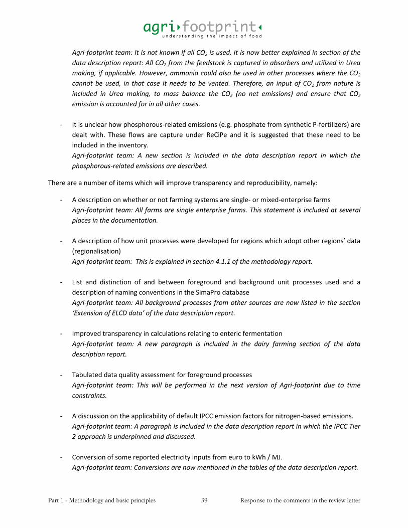
Part 1 - Methodology and basic principles 39 Response to the comments in the review letter

Agri-footprint team: It is not known if all CO2 is used. It is now better explained in section of the

data description report: All CO2 from the feedstock is captured in absorbers and utilized in Urea

making, if applicable. However, ammonia could also be used in other processes where the CO2

cannot be used, in that case it needs to be vented. Therefore, an input of CO2 from nature is

included in Urea making, to mass balance the CO2 (no net emissions) and ensure that CO2

emission is accounted for in all other cases.

- It is unclear how phosphorous-related emissions (e.g. phosphate from synthetic P-fertilizers) are

dealt with. These flows are capture under ReCiPe and it is suggested that these need to be

included in the inventory.

Agri-footprint team: A new section is included in the data description report in which the

phosphorous-related emissions are described.

There are a number of items which will improve transparency and reproducibility, namely:

- A description on whether or not farming systems are single- or mixed-enterprise farms

Agri-footprint team: All farms are single enterprise farms. This statement is included at several

places in the documentation.

- A description of how unit processes were developed for regions which adopt other regions’ data

(regionalisation)

Agri-footprint team: This is explained in section 4.1.1 of the methodology report.

- List and distinction of and between foreground and background unit processes used and a

description of naming conventions in the SimaPro database

Agri-footprint team: All background processes from other sources are now listed in the section

‘Extension of ELCD data’ of the data description report.

- Improved transparency in calculations relating to enteric fermentation

Agri-footprint team: A new paragraph is included in the dairy farming section of the data

description report.

- Tabulated data quality assessment for foreground processes

Agri-footprint team: This will be performed in the next version of Agri-footprint due to time

constraints.

- A discussion on the applicability of default IPCC emission factors for nitrogen-based emissions.

Agri-footprint team: A paragraph is included in the data description report in which the IPCC Tier

2 approach is underpinned and discussed.

- Conversion of some reported electricity inputs from euro to kWh / MJ.

Agri-footprint team: Conversions are now mentioned in the tables of the data description report.

Part 1 - Methodology and basic principles 40 Response to the comments in the review letter

- Data sources regarding assumptions for LTO operations for aircraft.

Agri-footprint team: The data source is ‘European Environment Agency (2006) Emission

Inventory Guidebook’ and is included in the air transport section of the data description report.

I have a number of suggestions which may improve usability of the methodology documents:

- System boundaries for each product type

Agri-footprint team: System boundaries for each product type are included in section 3.5.

- A list of environmental flows required for the target impact assessment method (ReCiPe)

Agri-footprint team: After consultation with RMIT it was decided that the added value was

limited. So this is not included in the reports.

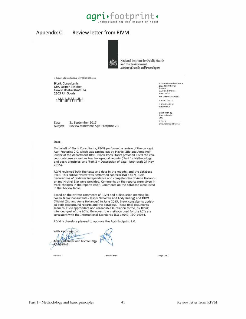
Part 1 - Methodology and basic principles 41 Review letter from RIVM

Review letter from RIVM Appendix C.

Part 1 - Methodology and basic principles 42 Self-declarations Agri-footprint 2.0 reviewers

Self-declarations Agri-footprint 2.0 reviewers Appendix D.

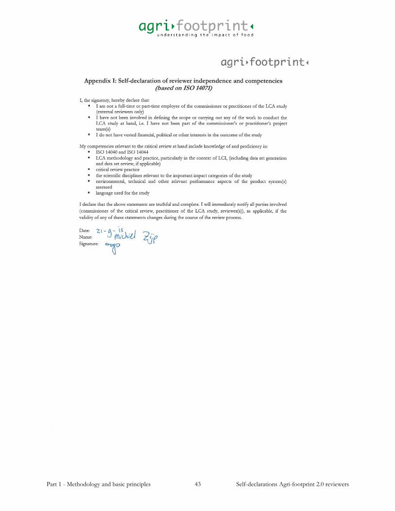
Part 1 - Methodology and basic principles 43 Self-declarations Agri-footprint 2.0 reviewers

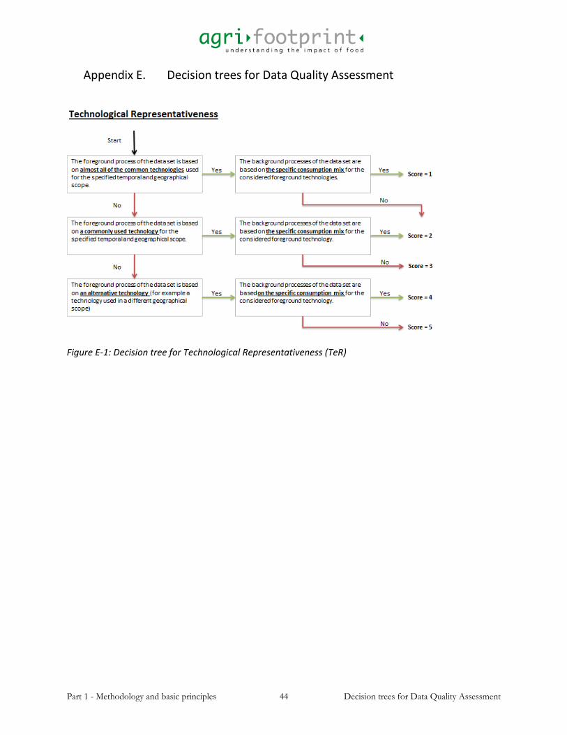
Part 1 - Methodology and basic principles 44 Decision trees for Data Quality Assessment

Decision trees for Data Quality Assessment Appendix E.

Figure E-1: Decision tree for Technological Representativeness (TeR)

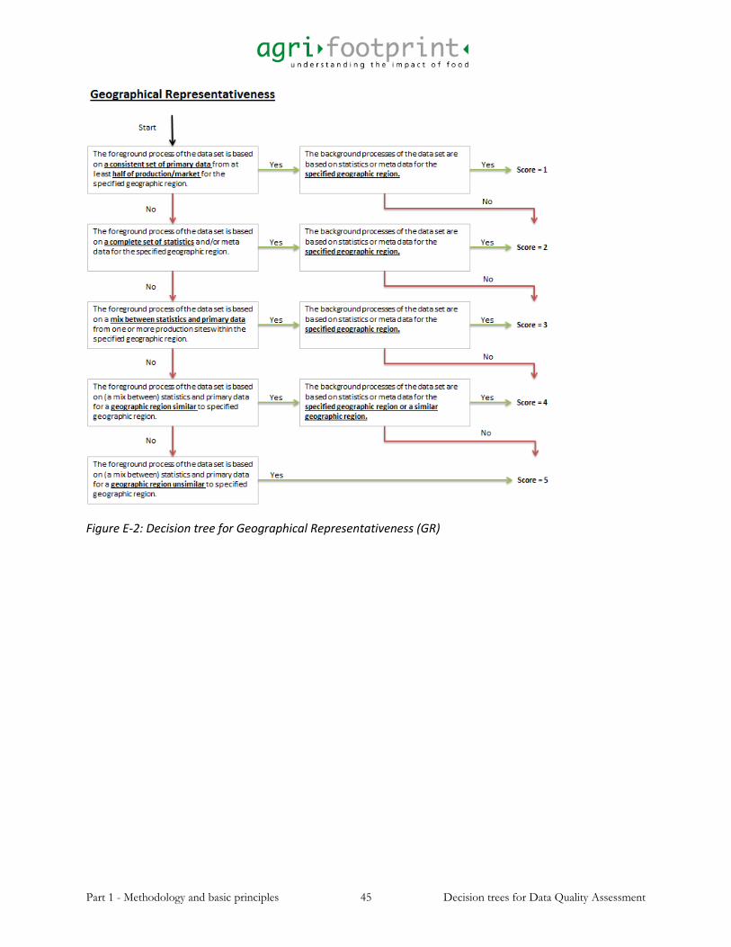
Part 1 - Methodology and basic principles 45 Decision trees for Data Quality Assessment

Figure E-2: Decision tree for Geographical Representativeness (GR)

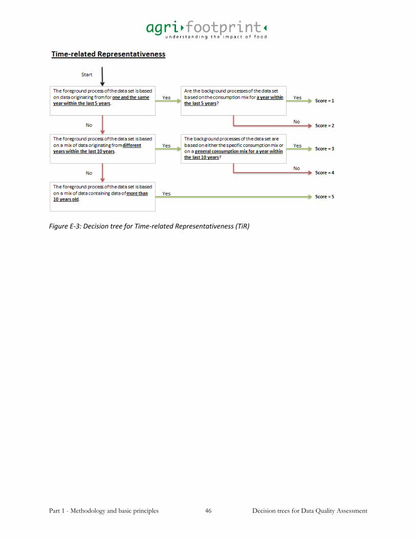
Part 1 - Methodology and basic principles 46 Decision trees for Data Quality Assessment

Figure E-3: Decision tree for Time-related Representativeness (TiR)

Part 1 - Methodology and basic principles 47 Decision trees for Data Quality Assessment

Figure E-4: Decision tree for Completeness (C)

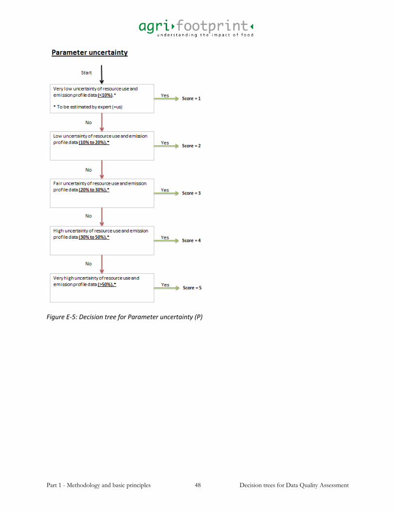
Part 1 - Methodology and basic principles 48 Decision trees for Data Quality Assessment

Figure E-5: Decision tree for Parameter uncertainty (P)

Part 1 - Methodology and basic principles 49 Decision trees for Data Quality Assessment

Figure E-6: Decision tree for methodological appropriateness and consistency (M)