Part 19: MLE Applications19-1/31

Econometrics IProfessor William Greene

Stern School of Business

Department of Economics

Part 19: MLE Applications19-2/31

Econometrics I

Part 19 –MLE Applications and a Two Step Estimator

Part 19: MLE Applications19-3/31

Model for a Binary Dependent Variable

Binary outcome. Event occurs or doesn’t (e.g., the democrat wins, the

person enters the labor force,… Model the probability of the event. P(x)=Prob(y=1|x) Probability responds to independent variables

Requirements 0 < Probability < 1 P(x) should be monotonic in x – it’s a CDF

Part 19: MLE Applications19-4/31

Two Standard Models Based on the normal distribution:

Prob[y=1|x] = (β’x) = CDF of normal distribution The “probit” model

Based on the logistic distribution Prob[y=1|x] = exp(β’x)/[1+ exp(β’x)] The “logit” model

Log likelihood P(y|x) = (1-F)(1-y) Fy where F = the cdf LogL = Σi (1-yi)log(1-Fi) + yilogFi

= Σi F[(2yi-1)β’x] since F(-t)=1-F(t) for both.

Part 19: MLE Applications19-5/31

Coefficients in the Binary Choice Models E[y|x] = 0*(1-Fi) + 1*Fi = P(y=1|x)

= F(β’x)

The coefficients are not the slopes, as usual

in a nonlinear model

∂E[y|x]/∂x= f(β’x)β

These will look similar for probit and logit

Part 19: MLE Applications19-6/31

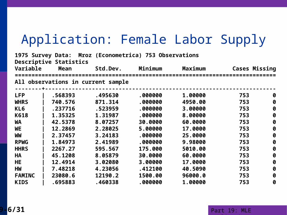
Application: Female Labor Supply1975 Survey Data: Mroz (Econometrica) 753 ObservationsDescriptive StatisticsVariable Mean Std.Dev. Minimum Maximum Cases Missing==============================================================================All observations in current sample--------+---------------------------------------------------------------------LFP | .568393 .495630 .000000 1.00000 753 0WHRS | 740.576 871.314 .000000 4950.00 753 0KL6 | .237716 .523959 .000000 3.00000 753 0K618 | 1.35325 1.31987 .000000 8.00000 753 0WA | 42.5378 8.07257 30.0000 60.0000 753 0WE | 12.2869 2.28025 5.00000 17.0000 753 0WW | 2.37457 3.24183 .000000 25.0000 753 0RPWG | 1.84973 2.41989 .000000 9.98000 753 0HHRS | 2267.27 595.567 175.000 5010.00 753 0HA | 45.1208 8.05879 30.0000 60.0000 753 0HE | 12.4914 3.02080 3.00000 17.0000 753 0HW | 7.48218 4.23056 .412100 40.5090 753 0FAMINC | 23080.6 12190.2 1500.00 96000.0 753 0KIDS | .695883 .460338 .000000 1.00000 753 0

Part 19: MLE Applications19-7/31

----------------------------------------------------------------------Binomial Probit ModelDependent variable LFPLog likelihood function -488.26476 (Probit)Log likelihood function -488.17640 (Logit)--------+-------------------------------------------------------------Variable| Coefficient Standard Error b/St.Er. P[|Z|>z] Mean of X--------+------------------------------------------------------------- |Index function for probabilityConstant| .77143 .52381 1.473 .1408 WA| -.02008 .01305 -1.538 .1241 42.5378 WE| .13881*** .02710 5.122 .0000 12.2869 HHRS| -.00019** .801461D-04 -2.359 .0183 2267.27 HA| -.00526 .01285 -.410 .6821 45.1208 HE| -.06136*** .02058 -2.982 .0029 12.4914 FAMINC| .00997** .00435 2.289 .0221 23.0806 KIDS| -.34017*** .12556 -2.709 .0067 .69588--------+-------------------------------------------------------------Binary Logit Model for Binary Choice--------+------------------------------------------------------------- |Characteristics in numerator of Prob[Y = 1]Constant| 1.24556 .84987 1.466 .1428 WA| -.03289 .02134 -1.542 .1232 42.5378 WE| .22584*** .04504 5.014 .0000 12.2869 HHRS| -.00030** .00013 -2.326 .0200 2267.27 HA| -.00856 .02098 -.408 .6834 45.1208 HE| -.10096*** .03381 -2.986 .0028 12.4914 FAMINC| .01727** .00752 2.298 .0215 23.0806 KIDS| -.54990*** .20416 -2.693 .0071 .69588--------+-------------------------------------------------------------

Estimated Choice Models for Labor Force Participation

Part 19: MLE Applications19-8/31

Partial Effects----------------------------------------------------------------------Partial derivatives of probabilities withrespect to the vector of characteristics.They are computed at the means of the Xs.Observations used are All Obs.--------+-------------------------------------------------------------Variable| Coefficient Standard Error b/St.Er. P[|Z|>z] Elasticity--------+------------------------------------------------------------- |PROBIT: Index function for probability WA| -.00788 .00512 -1.538 .1240 -.58479 WE| .05445*** .01062 5.127 .0000 1.16790 HHRS|-.74164D-04** .314375D-04 -2.359 .0183 -.29353 HA| -.00206 .00504 -.410 .6821 -.16263 HE| -.02407*** .00807 -2.983 .0029 -.52488 FAMINC| .00391** .00171 2.289 .0221 .15753 |Marginal effect for dummy variable is P|1 - P|0. KIDS| -.13093*** .04708 -2.781 .0054 -.15905Variable| Coefficient Standard Error b/St.Er. P[|Z|>z] Elasticity--------+------------------------------------------------------------- |LOGIT: Marginal effect for variable in probability WA| -.00804 .00521 -1.542 .1231 -.59546 WE| .05521*** .01099 5.023 .0000 1.18097 HHRS|-.74419D-04** .319831D-04 -2.327 .0200 -.29375 HA| -.00209 .00513 -.408 .6834 -.16434 HE| -.02468*** .00826 -2.988 .0028 -.53673 FAMINC| .00422** .00184 2.301 .0214 .16966 |Marginal effect for dummy variable is P|1 - P|0. KIDS| -.13120*** .04709 -2.786 .0053 -.15894--------+-------------------------------------------------------------

Part 19: MLE Applications19-9/31

I have a question. The question is as follows. We have a probit model. We used LM tests to test for the hetercodeaticiy in this model and found that there is heterocedasticity in this model...

How do we proceed now?  What do we do to get rid of heterescedasticiy?

Testing for heteroscedasticity in a probit model and then getting rid of heteroscedasticit in this model is not a common procedure. In fact I do not remember seen an applied (or theoretical also) works which tests for heteroscedasticiy and then uses a method to get rid of it???

See Econometric Analysis, 7th ed. pages 714-714

Part 19: MLE Applications19-10/31

2

11

21 1 1

1( | ) exp( / ),

exp( ) [ | ]; [ | ]

log ( | ) log

loglog 11

loNote since [ | ], E

i i i ii

i i i i i i i

n n ii i iii

i

n n ni i i ii i ii i i

i i i i

i i i

P y y

E y Var y

yLogL P y

L y yL

E y

x

x x x

x

x x

x

gL

0

Exponential Regression Model

Part 19: MLE Applications19-11/31

Variance of the First Derivative

1

1 1

1( | ) exp( / ),

log1

logNote since [ | ], E

log 1 1Var [ | ]

i i i ii

n iii

i

i i i

n n

i i i i i i ii ii i

P y y

yL

LE y

LVar y

22 2

x

x

x 0

x x x x x X X

Part 19: MLE Applications19-12/31

Hessian

1

2

21 1

2

1( | ) exp( / ),

log1

log

log because E[ | ]

i i i ii

n iii

i

n ni ii i i i ii i

i i

i i i

P y y

yL

y yL

LE y

x

x

x x x x

X X, x

Part 19: MLE Applications19-13/31

Variance Estimators

1

1

2

Negative inverse of actual second derivatives Matrix

ˆ ˆ, expˆ

Negative inverse of expected second derivatives

log

Sum of outer

n ii i i MLE ii

i

y

LE

-1

x x x

X X, so [X X]

1

1

1

1 1 1

products of first derivatives (BHHH)

1ˆ

"Robust" estimator in wide use

1ˆ ˆ ˆ

n ii ii

i

n n ni i ii i i i i ii i i

i i i

y

y y y

2

2

x x

x x x x x x

1

Part 19: MLE Applications19-14/31

Income Data

Fre

quency

H H N IN C

.000 .438 .876 1.314 1.753 2.191 2.629 3.067

Part 19: MLE Applications19-15/31

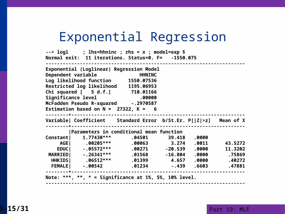
Exponential Regression--> logl ; lhs=hhninc ; rhs = x ; model=exp $Normal exit: 11 iterations. Status=0. F= -1550.075----------------------------------------------------------------------Exponential (Loglinear) Regression ModelDependent variable HHNINCLog likelihood function 1550.07536Restricted log likelihood 1195.06953Chi squared [ 5 d.f.] 710.01166Significance level .00000McFadden Pseudo R-squared -.2970587Estimation based on N = 27322, K = 6--------+-------------------------------------------------------------Variable| Coefficient Standard Error b/St.Er. P[|Z|>z] Mean of X--------+------------------------------------------------------------- |Parameters in conditional mean functionConstant| 1.77430*** .04501 39.418 .0000 AGE| .00205*** .00063 3.274 .0011 43.5272 EDUC| -.05572*** .00271 -20.539 .0000 11.3202 MARRIED| -.26341*** .01568 -16.804 .0000 .75869 HHKIDS| .06512*** .01399 4.657 .0000 .40272 FEMALE| -.00542 .01234 -.439 .6603 .47881--------+-------------------------------------------------------------Note: ***, **, * = Significance at 1%, 5%, 10% level.----------------------------------------------------------------------

Part 19: MLE Applications19-16/31

Variance Estimators

histogram;rhs=hhninc$reject ; hhninc=0$namelist ; X = one, age,educ,married,hhkids,female $loglinear ; lhs=hhninc ; rhs = x ; model=exp $create ; thetai = exp(b'x) $create ; gi = (hhninc/thetai - 1) ; gi2 = gi^2 $$create ; hi = (hhninc/thetai) $matrix ; Expected = <X'X> ; Stat(b,Expected,X)$matrix ; Actual = <X'[hi]X> ; Stat(b,Actual,X) $matrix ; BHHH = <X'[gi2]X> ; Stat(b,BHHH,X) $ matrix ; Robust = Actual * X'[gi2]X * Actual ; Stat(b,Robust,X) $

Part 19: MLE Applications19-17/31

Estimates

--------+--------------------------------------------------Variable| Coefficient Standard Error b/St.Er. P[|Z|>z]--------+----------------------------------------------------> matrix ; Expected = <X'X> ; Stat(b,Expected,X)$Constant| 1.77430*** .04548 39.010 .0000 AGE| .00205*** .00061 3.361 .0008 EDUC| -.05572*** .00269 -20.739 .0000 MARRIED| -.26341*** .01558 -16.902 .0000 HHKIDS| .06512*** .01425 4.571 .0000 FEMALE| -.00542 .01235 -.439 .6605--> matrix ; Actual = <X'[hi]X> ; Stat(b,Actual,X) $Constant| 1.77430*** .11922 14.883 .0000 AGE| .00205 .00181 1.137 .2553 EDUC| -.05572*** .00631 -8.837 .0000 MARRIED| -.26341*** .04954 -5.318 .0000 HHKIDS| .06512* .03920 1.661 .0967 FEMALE| -.00542 .03471 -.156 .8759--> matrix ; BHHH = <X'[gi2]X> ; Stat(b,BHHH,X) $Constant| 1.77430*** .05409 32.802 .0000 AGE| .00205*** .00069 2.973 .0029 EDUC| -.05572*** .00331 -16.815 .0000 MARRIED| -.26341*** .01737 -15.165 .0000 HHKIDS| .06512*** .01637 3.978 .0001 FEMALE| -.00542 .01410 -.385 .7004--> matrix ; Robust = Actual * X'[gi2]X * Actual $Constant| 1.77430*** .28500 6.226 .0000 AGE| .00205 .00481 .427 .6691 EDUC| -.05572*** .01306 -4.268 .0000 MARRIED| -.26341* .14581 -1.806 .0708 HHKIDS| .06512 .09459 .689 .4911 FEMALE| -.00542 .08580 -.063 .9496

Part 19: MLE Applications19-18/31

GARCH Models: A Model for Time Series with Latent Heteroscedasticity

Bollerslev/Ghysel, 1974

Part 19: MLE Applications19-19/31

ARCH Model

Part 19: MLE Applications19-20/31

GARCH Model

Part 19: MLE Applications19-21/31

Estimated GARCH Model----------------------------------------------------------------------GARCH MODELDependent variable YLog likelihood function -1106.60788Restricted log likelihood -1311.09637Chi squared [ 2 d.f.] 408.97699Significance level .00000McFadden Pseudo R-squared .1559676Estimation based on N = 1974, K = 4GARCH Model, P = 1, Q = 1Wald statistic for GARCH = 3727.503--------+-------------------------------------------------------------Variable| Coefficient Standard Error b/St.Er. P[|Z|>z] Mean of X--------+------------------------------------------------------------- |Regression parametersConstant| -.00619 .00873 -.709 .4783 |Unconditional VarianceAlpha(0)| .01076*** .00312 3.445 .0006 |Lagged Variance TermsDelta(1)| .80597*** .03015 26.731 .0000 |Lagged Squared Disturbance TermsAlpha(1)| .15313*** .02732 5.605 .0000 |Equilibrium variance, a0/[1-D(1)-A(1)]EquilVar| .26316 .59402 .443 .6577--------+-------------------------------------------------------------

Part 19: MLE Applications19-22/31

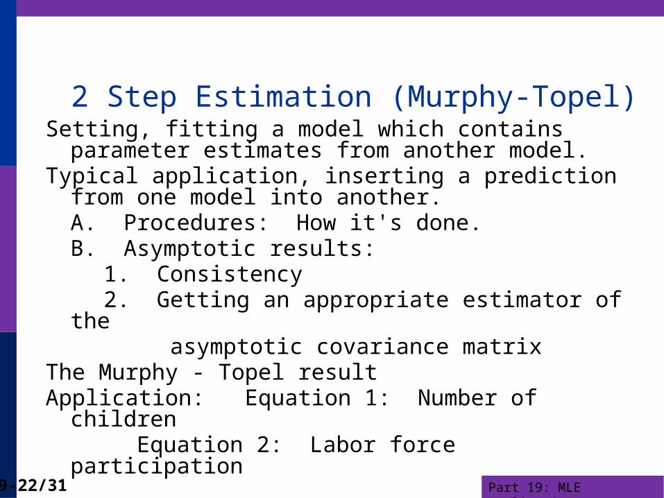
2 Step Estimation (Murphy-Topel)Setting, fitting a model which contains parameter estimates

from another model.Typical application, inserting a prediction from one model

into another.A. Procedures: How it's done.B. Asymptotic results:

1. Consistency2. Getting an appropriate estimator of the asymptotic covariance matrix

The Murphy - Topel resultApplication: Equation 1: Number of children

Equation 2: Labor force participation

Part 19: MLE Applications19-23/31

Setting

Two equation model: Model for y1 = f(y1 | x1, θ1)

Model for y2 = f(y2 | x2, θ2, x1, θ1) (Note, not ‘simultaneous’ or even ‘recursive.’)

Procedure: Estimate θ1 by ML, with covariance matrix (1/n)V1

Estimate θ2 by ML treating θ1 as if it were known. Correct the estimated asymptotic covariance matrix,

(1/n)V2 for the estimator of θ2

Part 19: MLE Applications19-24/31

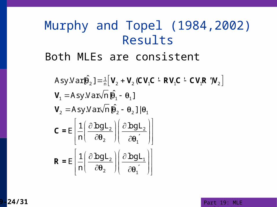
Murphy and Topel (1984,2002) Results Both MLEs are consistent

12 2 2 1 1 1 2n

1 1 1

2 2 2 1

2 2

2 1

2 1

2 1

ˆAsy.Var[ ] ( ' ' ')

ˆAsy.Var n[ ]

ˆAsy.Var n[ ] |

logL logL1E

n

logL logL1E

n

V V CV C RV C CVR V

V

V

C =

R =

Part 19: MLE Applications19-25/31

M&T Computations

H g g

H g g

1

1 1N N1 11 i 1 i1 i 1 i1 i1n n

2 1

1 1N N1 12 i 1 i2 i 1 i2 i3n n

ˆFirst equation: =MLE,

ˆˆ ˆ ˆ or

ˆ ˆSecond equation: =MLE|

ˆˆ ˆ ˆ or

V

V

C

R

N 2 2 2 2 1 1 2 2 2 2 1 1i 1

2 1

N 2 2 2 2 1 1 1 1 1 1i 1

2 1

ˆ ˆ ˆ ˆln f (y | , , , ) ln f (y | , , , )1 =

ˆ ˆn

ˆ ˆ ˆln f (y | , , , ) ln f (y | , )1 =

ˆ ˆn

x x x x

x x x

Part 19: MLE Applications19-26/31

Example

Equation 1: Number of Kids – Poisson Regression p(yi1|xi1, β)=exp(-λi)λi

yi1/yi1!

λi = exp(xi1’β)

gi1 = xi1(yi1 – λi)

V1 = [(1/n)Σ(-λi)xi1xi1’]-1

Part 19: MLE Applications19-27/31

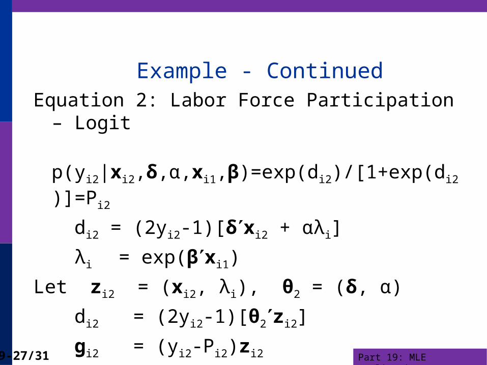
Example - ContinuedEquation 2: Labor Force Participation – Logit

p(yi2|xi2,δ,α,xi1,β)=exp(di2)/[1+exp(di2)]=Pi2

di2 = (2yi2-1)[δxi2 + αλi]

λi = exp(βxi1)

Let zi2 = (xi2, λi), θ2 = (δ, α)

di2 = (2yi2-1)[θ2zi2]

gi2 = (yi2-Pi2)zi2

V2 = [(1/n)Σ{-Pi2(1-Pi2)}zi2zi2’]-1

Part 19: MLE Applications19-28/31

Murphy and Topel Correction

N1i 1 i2 i2 i2 i2 i2 i i1N

N1i 1 i2 i2 i2 i1 i i1N

(y P ) (y P )

(y P ) (y )

C z x

R z x

Part 19: MLE Applications19-29/31

Two Step Estimation of LFP Model? Data transformations. Number of kids, scale income variablesCreate ; Kids = kl6 + k618 ; income = faminc/10000 ; Wifeinc = ww*whrs/1000 $? Equation 1, number of kids. Standard Poisson fertility model.? Fit equation, collect parameters BETA and covariance matrix V1? Then compute fitted values and derivativesNamelist ; X1 = one,wa,we,income,wifeinc$Poisson ; Lhs = kids ; Rhs = X1 $Matrix ; Beta = b ; V1 = N*VARB $Create ; Lambda = Exp(X1'Beta); gi1 = Kids - Lambda $? Set up logit labor force participation model? Compute probit model and collect results. Delta=Coefficients on X2? Alpha = coefficient on fitted number of kids. Namelist ; X2 = one,wa,we,ha,he,income ; Z2 = X2,Lambda $Logit ; Lhs = lfp ; Rhs = Z2 $Calc ; alpha = b(kreg) ; K2 = Col(X2) $Matrix ; delta=b(1:K2) ; Theta2 = b ; V2 = N*VARB $? Poisson derivative of with respect to beta is (kidsi - lambda)´X1Create ; di = delta'X2 + alpha*Lambda ; pi2= exp(di)/(1+exp(di)) ; gi2 = LFP - Pi2? These are the terms that are used to compute R and C. ; ci = gi2*gi2*alpha*lambda ; ri = gi2*gi1$MATRIX ; C = 1/n*Z2'[ci]X1 ; R = 1/n*Z2'[ri]X1 ; A = C*V1*C' - R*V1*C' - C*V1*R' ; V2S = V2+V2*A*V2 ; V2s = 1/N*V2S $? Compute matrix products and report resultsMatrix ; Stat(Theta2,V2s,Z2)$

Part 19: MLE Applications19-30/31

Estimated Equation 1: E[Kids]

+---------------------------------------------+| Poisson Regression || Dependent variable KIDS || Number of observations 753 || Log likelihood function -1123.627 |+---------------------------------------------++---------+--------------+----------------+--------+---------+----------+|Variable | Coefficient | Standard Error |b/St.Er.|P[|Z|>z] | Mean of X|+---------+--------------+----------------+--------+---------+----------+ Constant 3.34216852 .24375192 13.711 .0000 WA -.06334700 .00401543 -15.776 .0000 42.5378486 WE -.02572915 .01449538 -1.775 .0759 12.2868526 INCOME .06024922 .02432043 2.477 .0132 2.30805950 WIFEINC -.04922310 .00856067 -5.750 .0000 2.95163126

Part 19: MLE Applications19-31/31

Two Step Estimator+---------------------------------------------+| Multinomial Logit Model || Dependent variable LFP || Number of observations 753 || Log likelihood function -351.5765 || Number of parameters 7 |+---------------------------------------------++---------+--------------+----------------+--------+---------+----------+|Variable | Coefficient | Standard Error |b/St.Er.|P[|Z|>z] | Mean of X|+---------+--------------+----------------+--------+---------+----------+ Characteristics in numerator of Prob[Y = 1] Constant 33.1506089 2.88435238 11.493 .0000 WA -.54875880 .05079250 -10.804 .0000 42.5378486 WE -.02856207 .05754362 -.496 .6196 12.2868526 HA -.01197824 .02528962 -.474 .6358 45.1208499 HE -.02290480 .04210979 -.544 .5865 12.4913679 INCOME .39093149 .09669418 4.043 .0001 2.30805950 LAMBDA -5.63267225 .46165315 -12.201 .0000 1.59096946With Corrected Covariance Matrix+---------+--------------+----------------+--------+---------+|Variable | Coefficient | Standard Error |b/St.Er.|P[|Z|>z] |+---------+--------------+----------------+--------+---------+ Constant 33.1506089 5.41964589 6.117 .0000 WA -.54875880 .07780642 -7.053 .0000 WE -.02856207 .12508144 -.228 .8194 HA -.01197824 .02549883 -.470 .6385 HE -.02290480 .04862978 -.471 .6376 INCOME .39093149 .27444304 1.424 .1543 LAMBDA -5.63267225 1.07381248 -5.245 .0000