Embed Size (px)
Citation preview
Part 3 IE 312 1
Solving LP Models Improving Search
Unimodal Convex feasible region Should be successful!
Special Form of Improving Search Simplex method (now) Interior point methods (later)

Part 3 IE 312 2
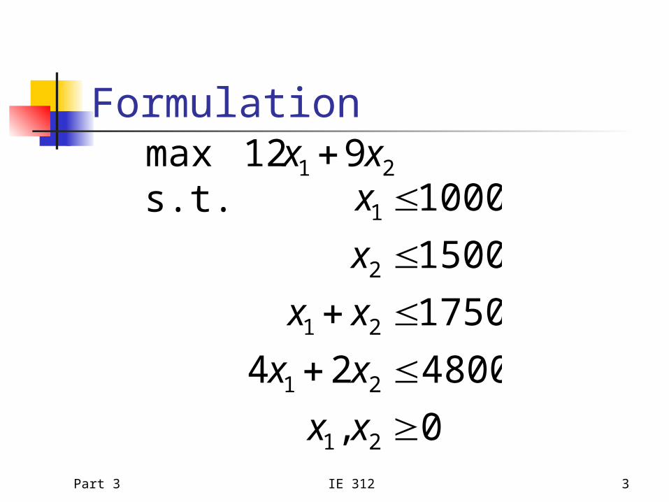
Simple Example Top Brass Trophy Company Makes trophies for
football wood base, engraved plaque, brass football on top $12 profit and uses 4’ of wood
soccer wood base, engraved plaque, soccer ball on top $9 profit and uses 2’ of wood
Current stock 1000 footballs, 1500 soccer balls, 1750
plaques, and 4800 feet of wood
Part 3 IE 312 3
Formulation
0,
480024
1750
1500
1000s.t.912max
21
21
21
2
1
21
xx
xx
xx
x
xxx
Part 3 IE 312 4
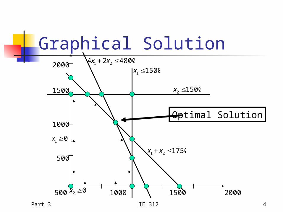
Graphical Solution2000
1500
1000
500
500 1000 1500 2000
15002 x
15001 x
175021 xx
480024 21 xx
01 x
02 x
Optimal Solution
Part 3 IE 312 5
Feasible Solutions Feasible solution is a
boundary point if at least one inequality constraint that can be strict is active
interior point if no such constraints are active
Extreme points of convex sets do not lie within the line segment of any other points in the set

Part 3 IE 312 6
Example2000
1500
1000
500
500 1000 1500 2000

Part 3 IE 312 7
Optimal Solutions Every optimal solution is a boundary
point We can find an improving direction whenever
we are at an interior point
If optimum unique the it must be an extreme point of the feasible region
If optimal solution exist, an optimal extreme point exists
Part 3 IE 312 8
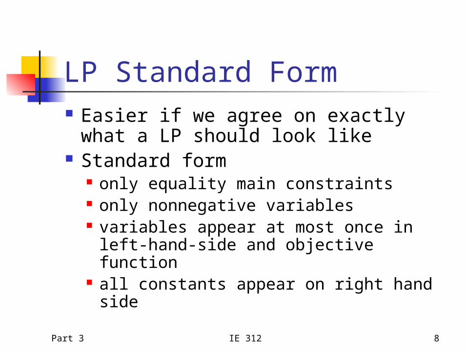
LP Standard Form Easier if we agree on exactly what
a LP should look like Standard form
only equality main constraints only nonnegative variables variables appear at most once in left-
hand-side and objective function all constants appear on right hand
side
Part 3 IE 312 9
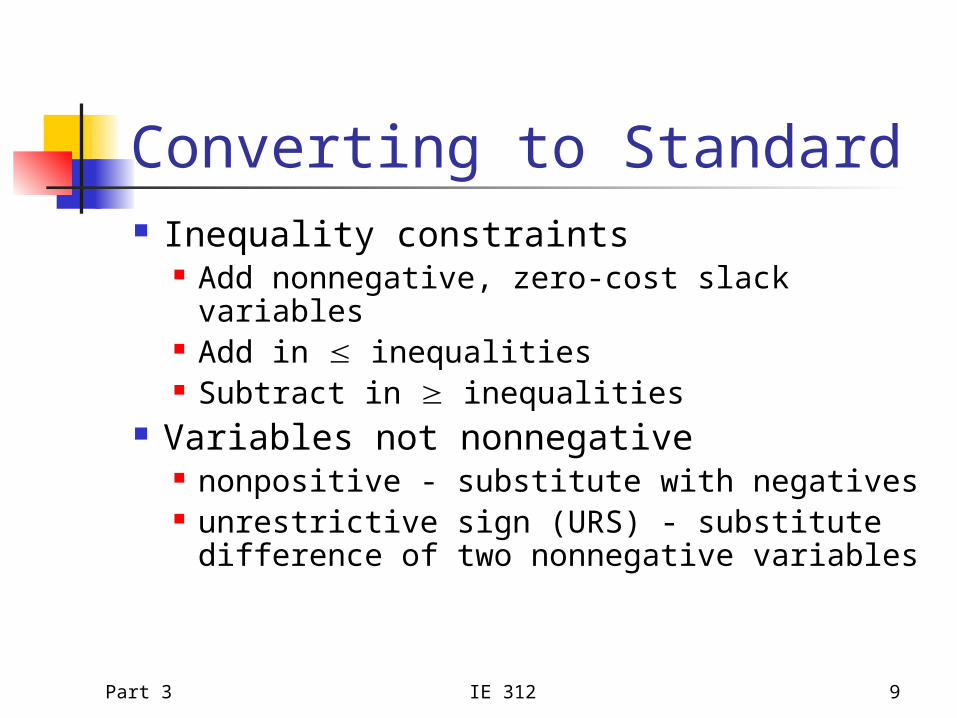
Converting to Standard Inequality constraints
Add nonnegative, zero-cost slack variables
Add in inequalities Subtract in inequalities
Variables not nonnegative nonpositive - substitute with negatives unrestrictive sign (URS) - substitute
difference of two nonnegative variables
Part 3 IE 312 10
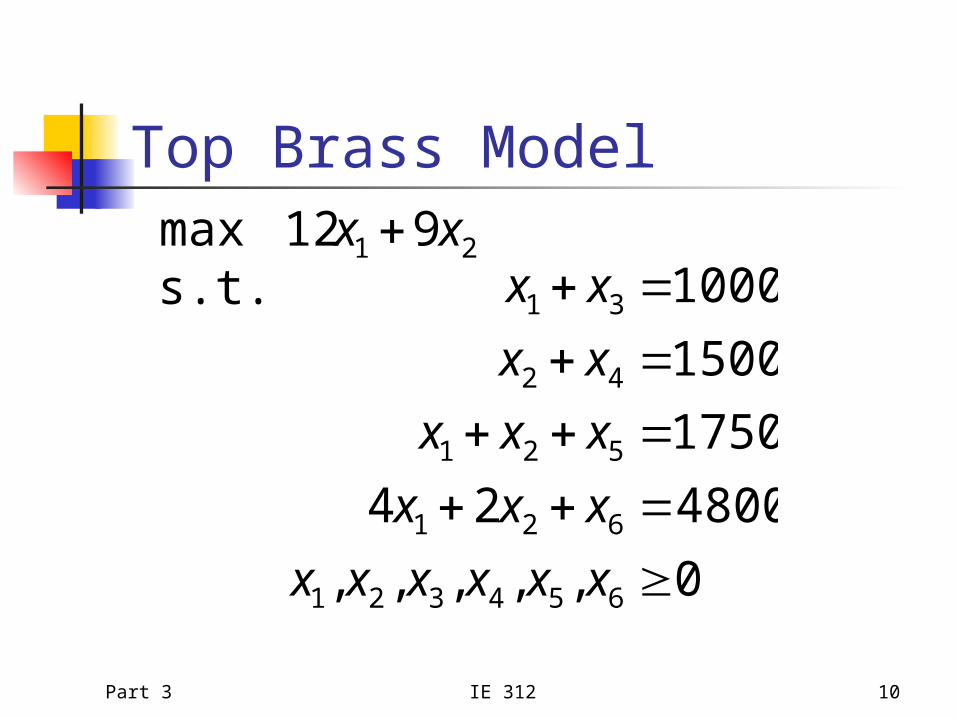
Top Brass Model
0,,,,,
480024
1750
1500
1000s.t.912max
654321
621
521
42
31
21
xxxxxx
xxx
xxx
xx
xxxx
Part 3 IE 312 11
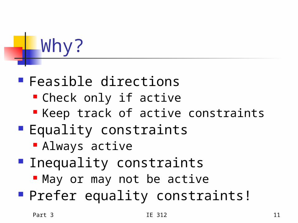
Why?
Feasible directions Check only if active Keep track of active constraints
Equality constraints Always active
Inequality constraints May or may not be active
Prefer equality constraints!
Part 3 IE 312 12
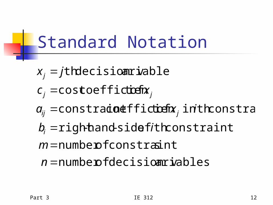
Standard Notation
ariablesdecision v ofnumber
sconstraint ofnumber
constraintth of side-hand-right
constraintth in oft coefficien constraint
oft coefficiencost
ariabledecision vth
n
m
ib
ixa
xc
jx
i
jij
jj
j
Part 3 IE 312 13
LP Standard Form
jx
ibxa
xc
j
n
jjjij
m
jjj
,0
,s.t.
maxmin/
1
1
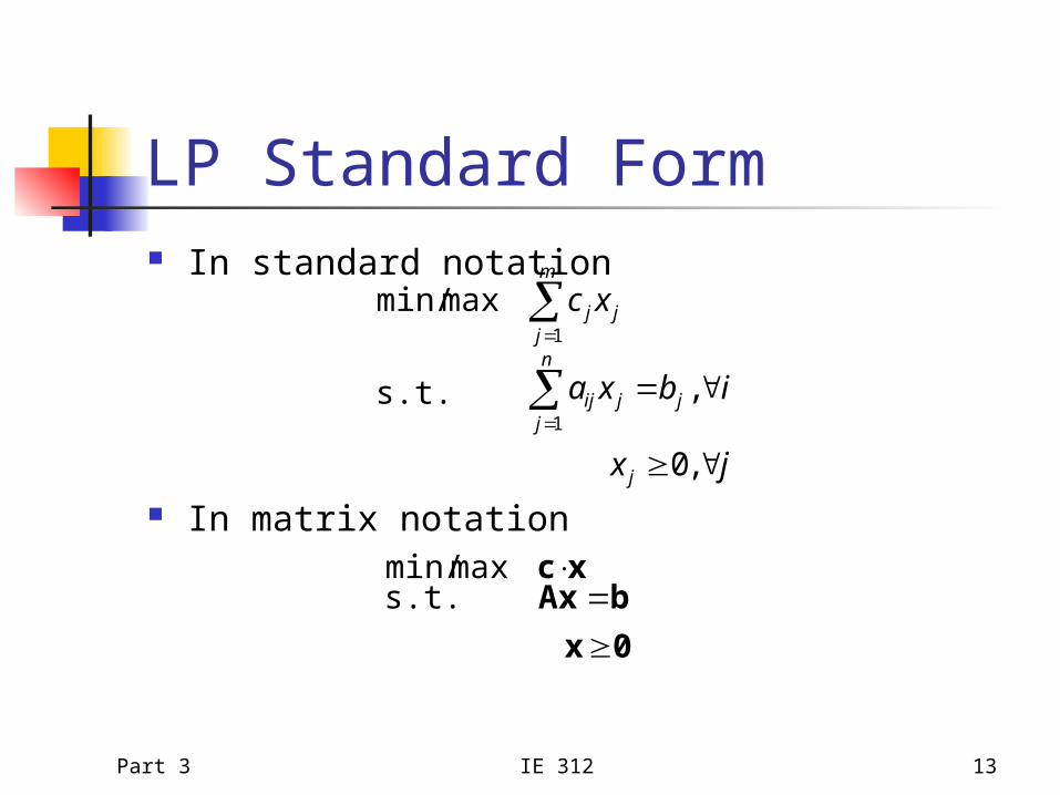
In standard notation
In matrix notation
0x
bAxxc
s.t.
maxmin/

Part 3 IE 312 14
Write in Matrix Form1 2 3
1 2 3 4
1 3 5
2 3
1 2 3 4 5
max 30 120 4
2 5 55s.t.
0
2 18 50
, , , , 0
x x x
x x x x
x x x
x x
x x x x x
bA
c
)(
Part 3 IE 312 15
Extreme Points Know that an extreme point
optimum exists Will search trough extreme points
An extreme point is define by a set of constraints that are active simultaneously

Part 3 IE 312 16
Improving Search Move from one extreme point to a
neighboring extreme point Extreme points are adjacent if they
are defined by sets of active constraints that differ by only one element
An edge is a line segment determined by a set of active constraints
Part 3 IE 312 17
Basic Solutions Extreme points are defined by set
of active nonnegativity constraints
A basic solution is a solution that is obtained by fixing enough variable to be equal to zero, so that the equality constraints have a unique solution
Part 3 IE 312 18
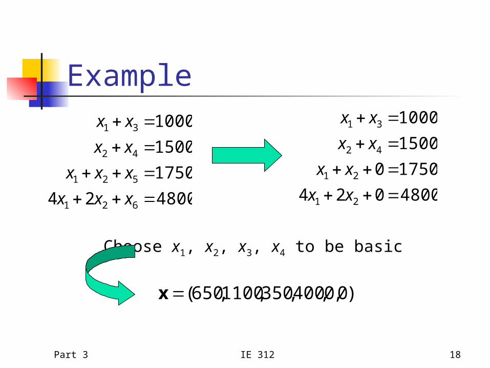
Example
480024
1750
1500
1000
621
521
42
31
xxx
xxx
xx
xx
4800024
17500
1500
1000
21
21
42
31
xx
xx
xx
xx
Choose x1, x2, x3, x4 to be basic
)0,0,400,350,1100,650(x
Part 3 IE 312 19
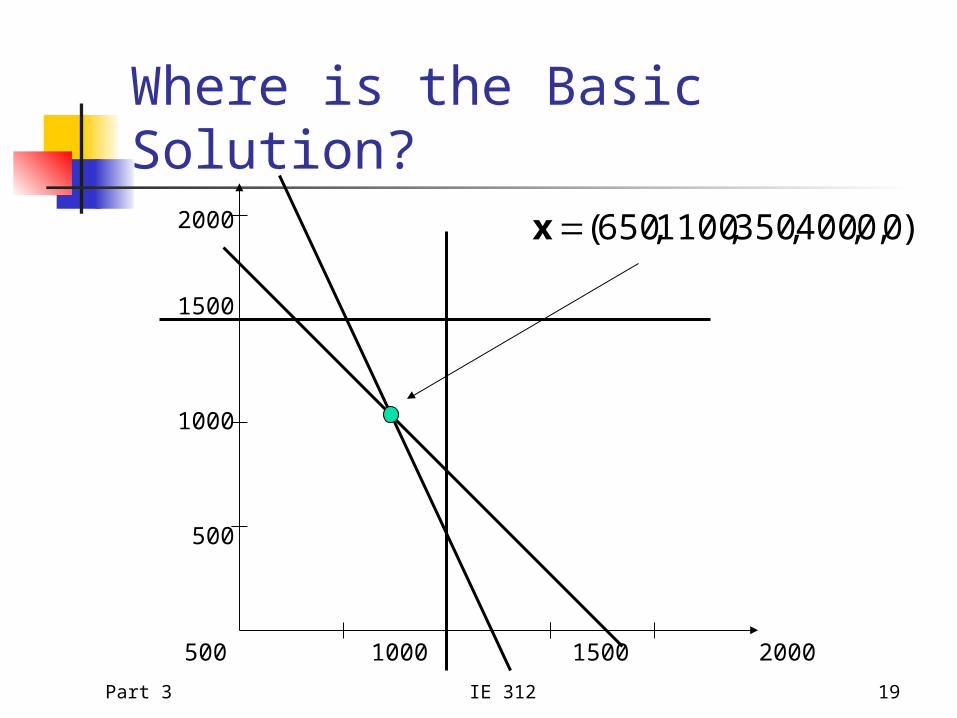
Where is the Basic Solution?2000
1500
1000
500
500 1000 1500 2000
)0,0,400,350,1100,650(x

Part 3 IE 312 20
Example
Compute the basic solution for x1 and x2 basis:
Solve
0,,,
8223
14
321
321
321
xxx
xxx
xxx
823
14
21
21
xx
xx3
1
2
1
x
x
Part 3 IE 312 21
Existence of Basis Solutions
Remember linear algebra?
A basis solution exists if and only if the columns of corresponding equality constraint form a basis(in other words, a largest possible linearly independent collection)
Part 3 IE 312 22
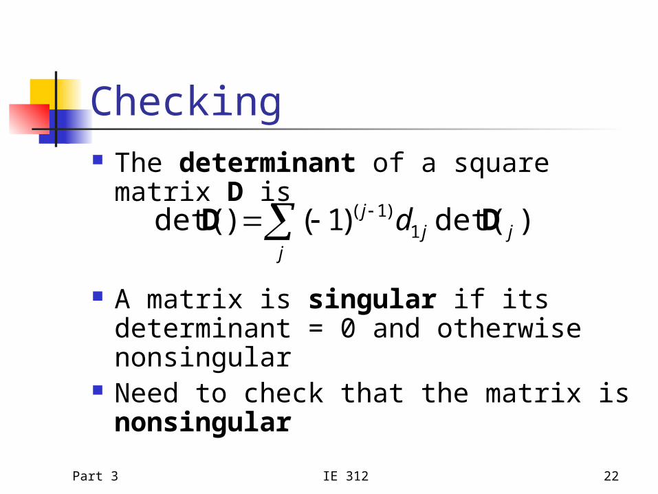
Checking The determinant of a square
matrix D is
A matrix is singular if its determinant = 0 and otherwise nonsingular
Need to check that the matrix is nonsingular
j
jjj d )det()1()det( 1
)1( DD
Part 3 IE 312 23
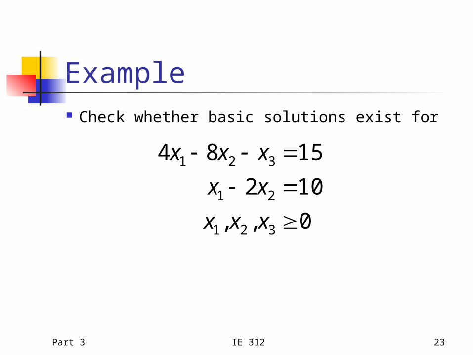
Example Check whether basic solutions exist for
0,,
102
1584
321
21
321
xxx
xx
xxx
Part 3 IE 312 24
Basic Feasible Solutions A basic feasible solution to a LP
is a basic solution that satisfies all the nonnegativity contraints
The basic feasible solutions correspond exactly to the extreme points of the feasible region
Part 3 IE 312 25
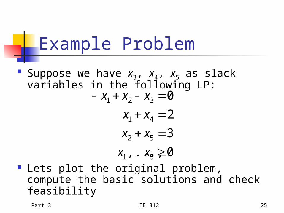
Example Problem Suppose we have x3, x4, x5 as slack
variables in the following LP:
Lets plot the original problem, compute the basic solutions and check feasibility
0,...,
3
2
0
51
52
41
321
xx
xx
xx
xxx
Part 3 IE 312 26
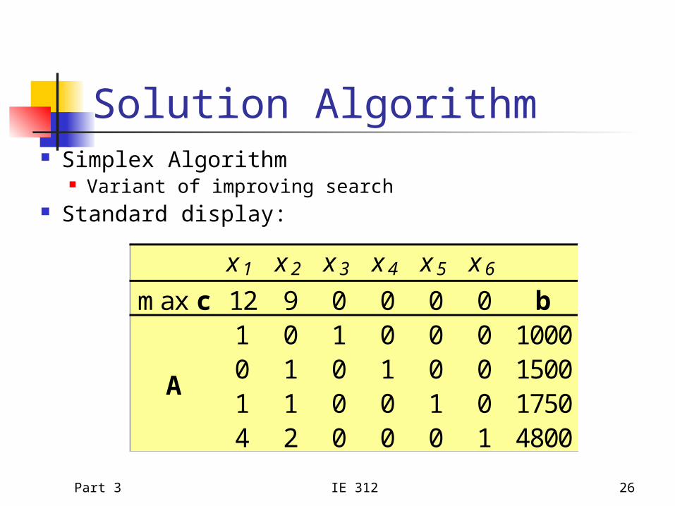
Solution Algorithm Simplex Algorithm
Variant of improving search Standard display:
x1 x2 x3 x4 x5 x6max c 12 9 0 0 0 0 b
1 0 1 0 0 0 10000 1 0 1 0 0 15001 1 0 0 1 0 17504 2 0 0 0 1 4800
A

Part 3 IE 312 27
Simplex Algorithm Starting point
A basic feasible solution (extreme point) Direction
Follow an edge to adjacent extreme point: Increase one nonbasic variable Compute changes needed to preserve
equality constraints One direction for each nonbasic variable
Part 3 IE 312 28
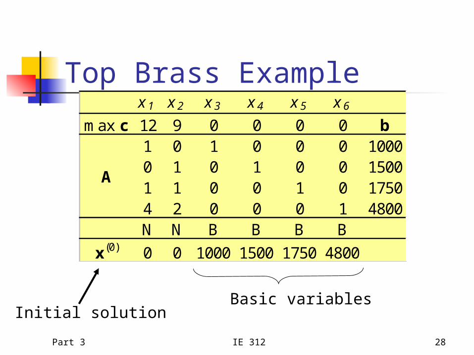
Top Brass Examplex 1 x 2 x 3 x 4 x 5 x 6
max c 12 9 0 0 0 0 b1 0 1 0 0 0 10000 1 0 1 0 0 15001 1 0 0 1 0 17504 2 0 0 0 1 4800N N B B B B
x(0) 0 0 1000 1500 1750 4800
A
Initial solutionBasic variables
Part 3 IE 312 29
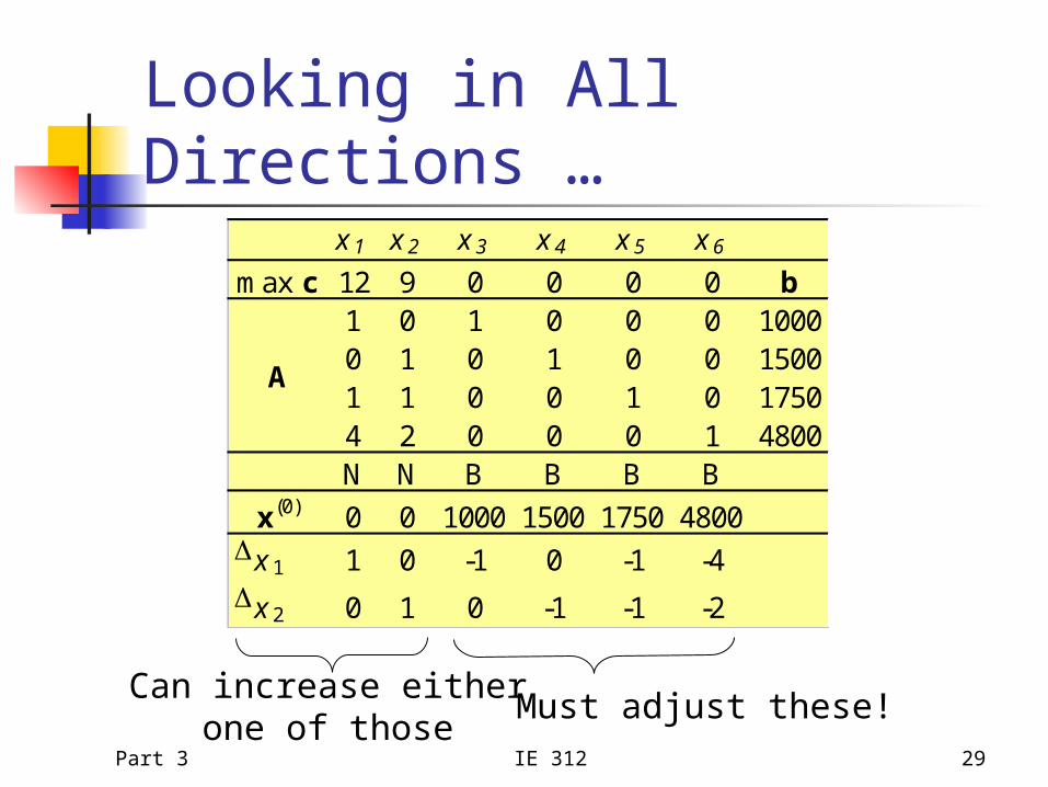
Looking in All Directions …x 1 x 2 x 3 x 4 x 5 x 6
max c 12 9 0 0 0 0 b1 0 1 0 0 0 10000 1 0 1 0 0 15001 1 0 0 1 0 17504 2 0 0 0 1 4800N N B B B B
x(0) 0 0 1000 1500 1750 4800Dx 1 1 0 -1 0 -1 -4
Dx 2 0 1 0 -1 -1 -2
A
Must adjust these!Can increase either
one of those
Part 3 IE 312 30
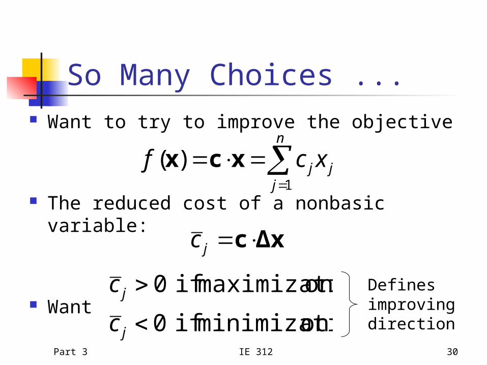
So Many Choices ... Want to try to improve the objective
The reduced cost of a nonbasic variable:
Want
n
jjj xcf
1
)( xcx
Δxcjc
onminimizati if 0
onmaximizati if 0
j
j
c
c Definesimprovingdirection
Part 3 IE 312 31
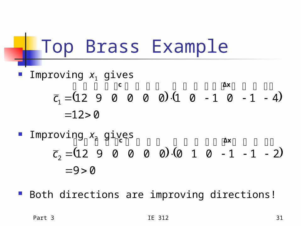
Top Brass Example Improving x1 gives
Improving x2 gives
Both directions are improving directions!
012
41010100009121
Δxc
c
09
21101000009122
Δxc
c

Part 3 IE 312 32
Where and How Far? Any improving direction will do If no component is negative Improve forever - unbounded!
Otherwise, compute the minimum ratio
DD
0:min)(
jj
tj xx
x

Part 3 IE 312 33
Computing Minimum Ratiox1 x2 x3 x4 x5 x6N N B B B B
x(0) 0 0 1000 1500 1750 4800Dx 1 0 -1 0 -1 -4
1000 1750 4800-(-1) -(-1) -(-4)
10004
4800,
1
1750,
1
1000min
0:min)(
DD
jj
tj xx
x

Part 3 IE 312 34
Moving to New Solution
480017501500000100
4101011000
480017501500100000
)0()1(
D xxx
Part 3 IE 312 35
Updating Basis
New basic variable
Nonbasic variable generating
direction
New nonbasic variable(s)
Basic variables fixing the step size
Part 3 IE 312 36
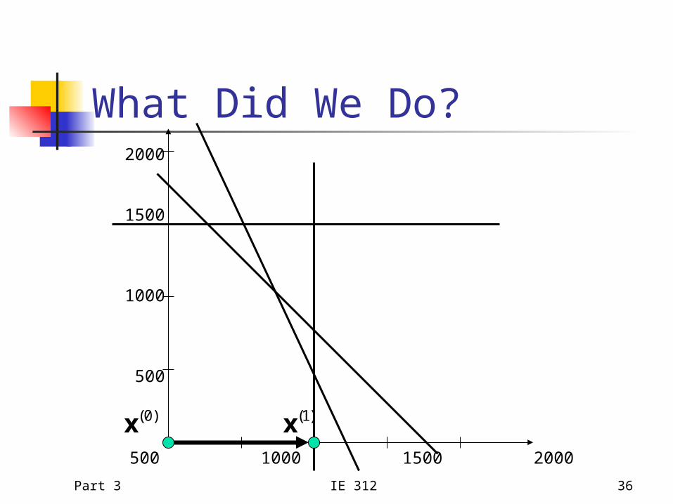
What Did We Do?2000
1500
1000
500
500 1000 1500 2000
)0(x )1(x
Part 3 IE 312 37
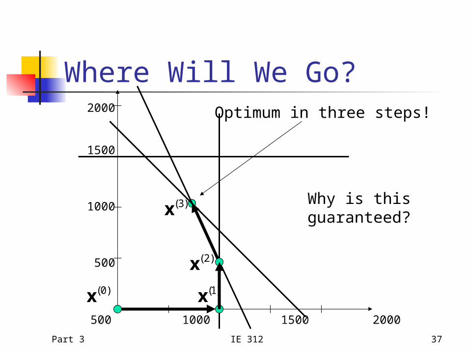
Where Will We Go?2000
1500
1000
500
500 1000 1500 2000
)0(x )1(x
Why is thisguaranteed?
)2(x
)3(x
Optimum in three steps!
Part 3 IE 312 38
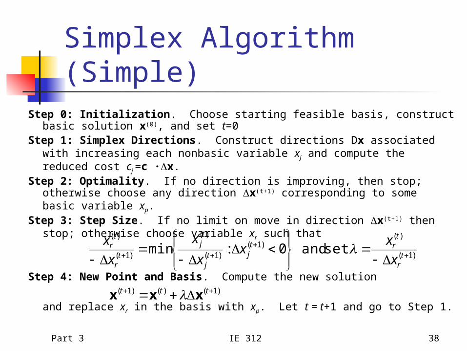
Simplex Algorithm (Simple)
Step 0: Initialization. Choose starting feasible basis, construct basic solution x(0), and set t=0
Step 1: Simplex Directions. Construct directions Dx associated with increasing each nonbasic variable xj and compute the reduced cost cj =c ·Dx.
Step 2: Optimality. If no direction is improving, then stop; otherwise choose any direction Dx(t+1) corresponding to some basic variable xp.
Step 3: Step Size. If no limit on move in direction Dx(t+1) then stop; otherwise choose variable xr such that
Step 4: New Point and Basis. Compute the new solution
and replace xr in the basis with xp. Let t = t+1 and go to Step 1.
)1(
)()1(
)1(
)(
)1(
)(
set and 0:min
D
DD
D t
r
trt
jtj
tj
tr
tr
x
xx
x
x
x
x
)1()()1( D ttt xxx
Part 3 IE 312 39
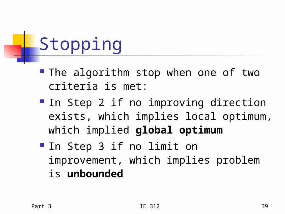
Stopping The algorithm stop when one of two
criteria is met: In Step 2 if no improving direction
exists, which implies local optimum, which implied global optimum
In Step 3 if no limit on improvement, which implies problem is unbounded
Part 3 IE 312 40
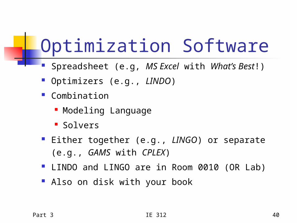
Optimization Software Spreadsheet (e.g, MS Excel with What’s Best!) Optimizers (e.g., LINDO) Combination
Modeling Language Solvers
Either together (e.g., LINGO) or separate (e.g., GAMS with CPLEX)
LINDO and LINGO are in Room 0010 (OR Lab) Also on disk with your book
Part 3 IE 312 41
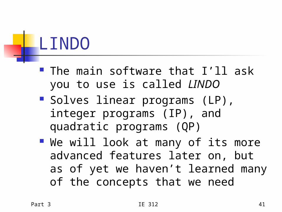
LINDO The main software that I’ll ask you to use is
called LINDO Solves linear programs (LP), integer
programs (IP), and quadratic programs (QP) We will look at many of its more advanced
features later on, but as of yet we haven’t learned many of the concepts that we need
Part 3 IE 312 42
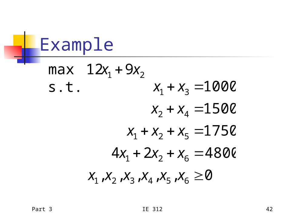
Example
0,,,,,
480024
1750
1500
1000s.t.912max
654321
621
521
42
31
21
xxxxxx
xxx
xxx
xx
xxxx
Part 3 IE 312 43
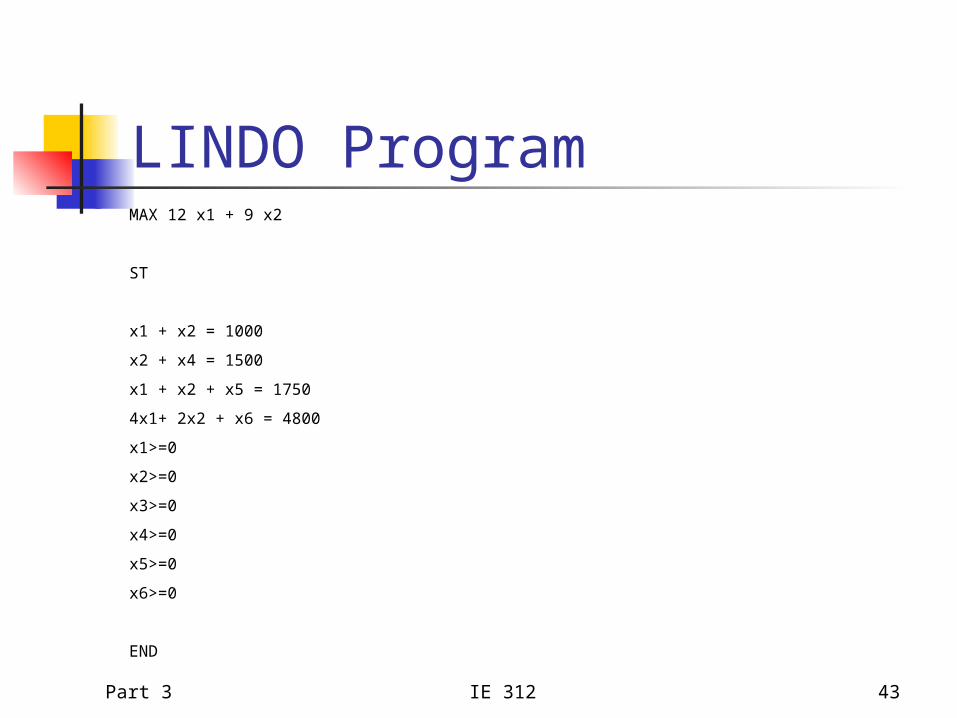
LINDO ProgramMAX 12 x1 + 9 x2
ST
x1 + x2 = 1000
x2 + x4 = 1500
x1 + x2 + x5 = 1750
4x1+ 2x2 + x6 = 4800
x1>=0
x2>=0
x3>=0
x4>=0
x5>=0
x6>=0
END
Part 3 IE 312 44

Part 3 IE 312 45
Part 3 IE 312 46
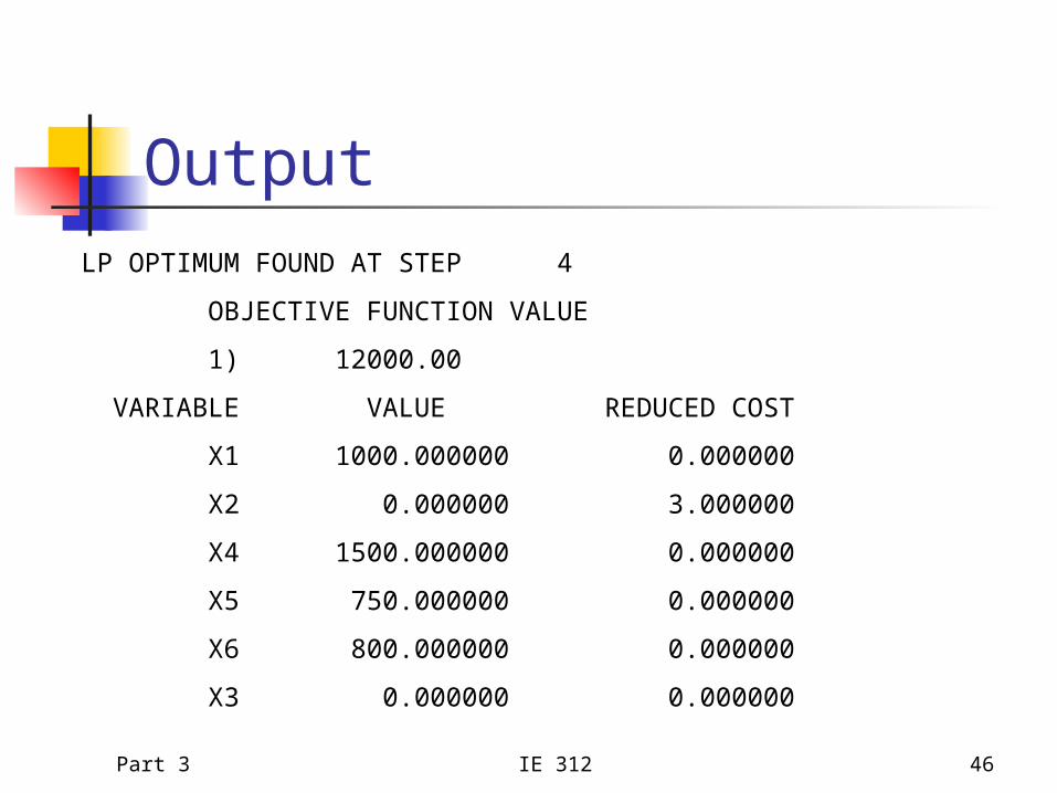
OutputLP OPTIMUM FOUND AT STEP 4
OBJECTIVE FUNCTION VALUE
1) 12000.00
VARIABLE VALUE REDUCED COST
X1 1000.000000 0.000000
X2 0.000000 3.000000
X4 1500.000000 0.000000
X5 750.000000 0.000000
X6 800.000000 0.000000
X3 0.000000 0.000000
Part 3 IE 312 47
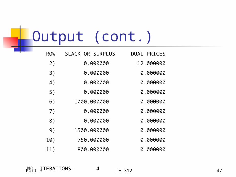
Output (cont.) ROW SLACK OR SURPLUS DUAL PRICES
2) 0.000000 12.000000
3) 0.000000 0.000000
4) 0.000000 0.000000
5) 0.000000 0.000000
6) 1000.000000 0.000000
7) 0.000000 0.000000
8) 0.000000 0.000000
9) 1500.000000 0.000000
10) 750.000000 0.000000
11) 800.000000 0.000000
NO. ITERATIONS= 4
Part 3 IE 312 48
LINDO: Basic Syntax Objective Function Syntax: Start all
models with MAX or MIN Variable Names: Limited to 8
characters Constraint Name: Terminated with a
parenthesis Recognized Operators (+, -, >, <, =) Order of Precedence: Parentheses not
recognized
Part 3 IE 312 49
Syntax (cont.) Adding Comment: Start with an
exclamation mark Splitting lines in a model: Permitted in
LINDO Case Sensitivity: LINDO has none Right-hand Side Syntax: Only constant
values Left-hand Side Syntax: Only variables
and their coefficients
Part 3 IE 312 50
Why Modeling Language? More to learn! More ‘complicated’ to use than
LINDO (at least at first glance) Advantages
Natural representations Similar to mathematical notation Can enter many terms simultaneously Much faster and easier to read
Part 3 IE 312 51
Why Solvers?
Best commercial software has modeling
language and solvers separated
Advantages: Select solver that is best for your application
Learn one modeling language use any solver
Buy 3rd party solvers or write your own!

Part 3 IE 312 52
Example ProblemBisco’s new sugar-free, fat-free chocolate squares are so popular that the companycnnot keep up with demand. Regional demands shown in the following table total2000 cases per week, but Bisco can produce only 60% of that number.
NE SE MW W
Demand 620 490 510 380
Profit 1.6 1.4 1.9 1.2
The table also shows the different profit levels per case experienced in the regionsdue to competition and consumer tastes. Bisco wants to find a maximum profitplan that fulfills between 50% and 70% of each region’s demand.

Part 3 IE 312 53
Problem Formulation
4,3,2,1,
1200
max
4
1
4
1
iuxl
x
xp
iii
ii
iii
Part 3 IE 312 54
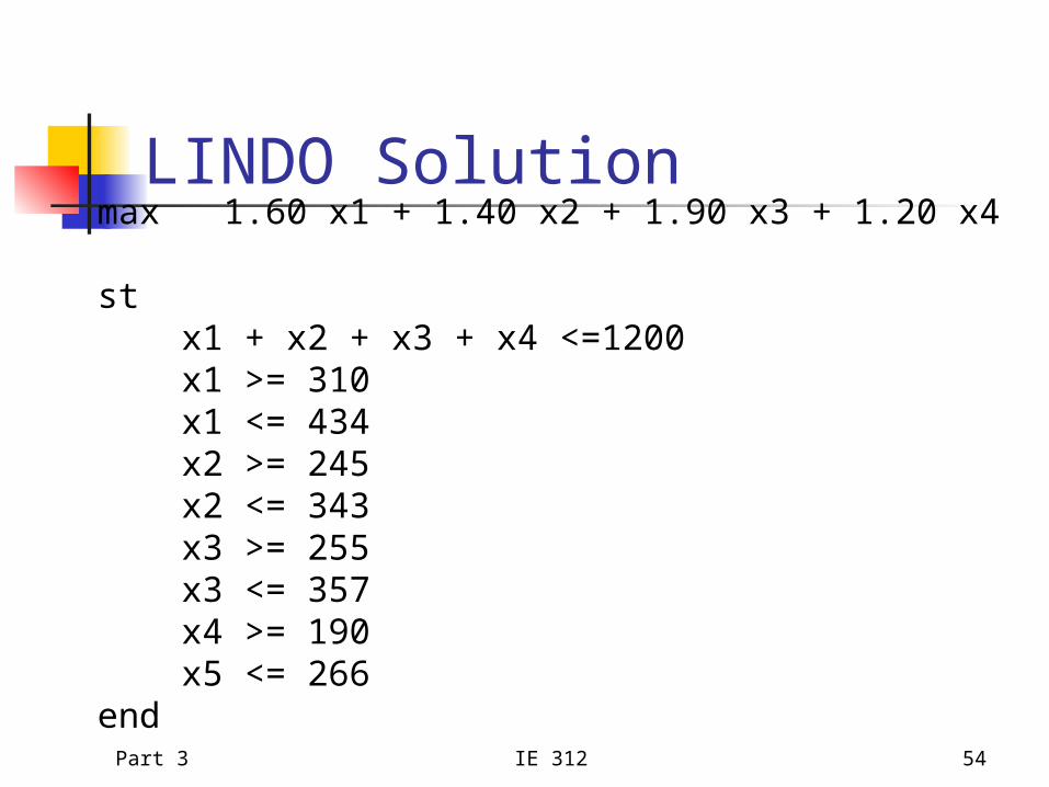
LINDO Solutionmax 1.60 x1 + 1.40 x2 + 1.90 x3 + 1.20 x4
st x1 + x2 + x3 + x4 <=1200 x1 >= 310 x1 <= 434 x2 >= 245 x2 <= 343 x3 >= 255 x3 <= 357 x4 >= 190 x5 <= 266end
Part 3 IE 312 55
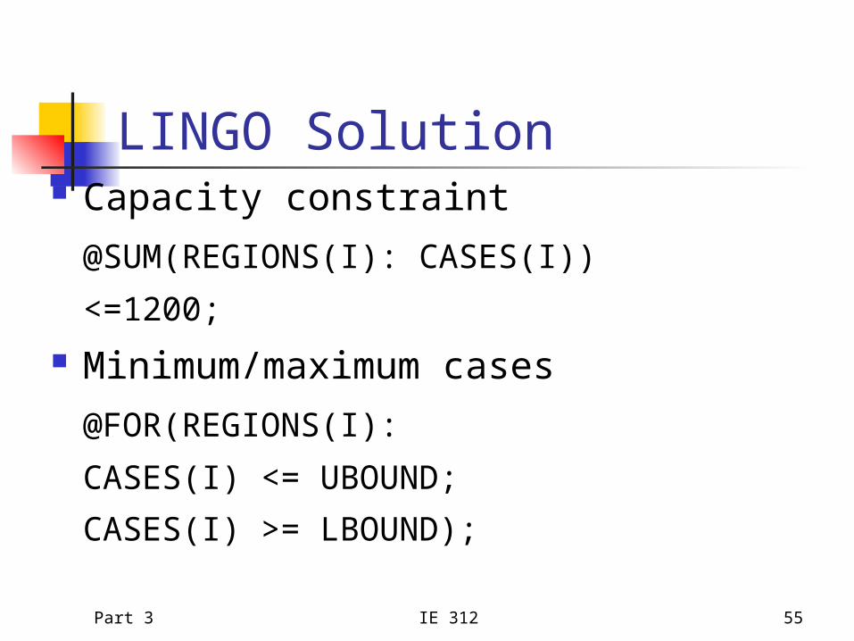
LINGO Solution Capacity constraint
@SUM(REGIONS(I): CASES(I))
<=1200;
Minimum/maximum cases
@FOR(REGIONS(I):
CASES(I) <= UBOUND;
CASES(I) >= LBOUND);
Part 3 IE 312 56
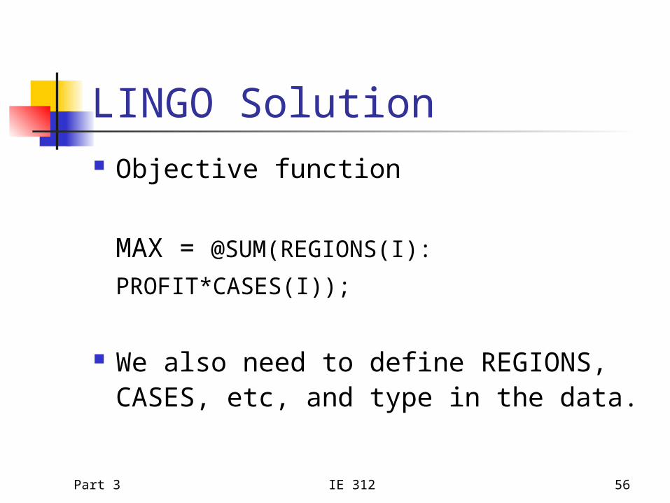
LINGO Solution Objective function
MAX = @SUM(REGIONS(I): PROFIT*CASES(I));
We also need to define REGIONS, CASES, etc, and type in the data.
Part 3 IE 312 57
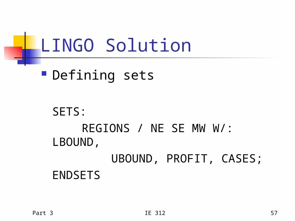
LINGO Solution Defining sets
SETS:
REGIONS / NE SE MW W/: LBOUND,
UBOUND, PROFIT, CASES;
ENDSETS

Part 3 IE 312 58
LINGO Solution Enter the data
DATA:
LBOUND = 310 245 255 190;
UBOUND = 434 343 357 266;
PROFIT = 1.6 1.4 1.9 1.2;
ENDDATA
Part 3 IE 312 59
Sensitivity Analysis Basic Question: How does our solution
change as the input parameters change? The objective function?
More/less profit or cost The optimal values of decision variables?
Make different decisions!
Why? Only have estimates of input parameters May want to change input parameters
Part 3 IE 312 60
What We Know Qualitative Answers for All Problems Quantitative Answers for Linear
Programs (LP) Dual program Same input parameters Decision variables give sensitivities Dual prices Easy to set up Theory is somewhat complicated

Part 3 IE 312 61
Back to Example Problem
Bisco’s new sugar-free, fat-free chocolate squares are so popular that the companycnnot keep up with demand. Regional demands shown in the following table total2000 cases per week, but Bisco can produce only 60% of that number.
NE SE MW W
Demand 620 490 510 380
Profit 1.6 1.4 1.9 1.2
The table also shows the different profit levels per case experienced in the regionsdue to competition and consumer tastes. Bisco wants to find a maximum profitplan that fulfills between 50% and 70% of each region’s demand.

Part 3 IE 312 62
LINDO Formulation
max 1.60 x1 + 1.40 x2 + 1.90 x3 + 1.20 x4
st
x1 + x2 + x3 + x4 <=1200
x1 >= 310
x1 <= 434
x2 >= 245
x2 <= 343
x3 >= 255
x3 <= 357
x4 >= 190
x5 <= 266
end
Part 3 IE 312 63
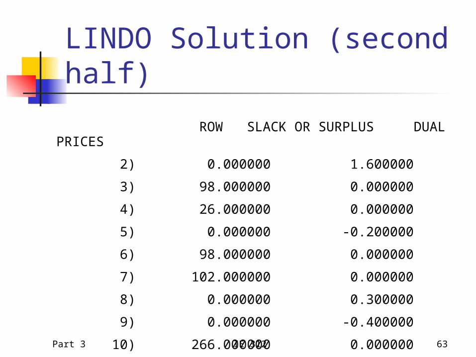
LINDO Solution (second half)
ROW SLACK OR SURPLUS DUAL PRICES
2) 0.000000 1.600000
3) 98.000000 0.000000
4) 26.000000 0.000000
5) 0.000000 -0.200000
6) 98.000000 0.000000
7) 102.000000 0.000000
8) 0.000000 0.300000
9) 0.000000 -0.400000
10) 266.000000 0.000000
Part 3 IE 312 64
Dual Prices The Dual is Automatically Formed
Also in LINGO Also in (all) other optimization software
Report dual prices Gives us sensitivities to RHS parameter Know how much objective function will
change When will the optimal solution change? Need to select that we want sensitivity
analysis
Part 3 IE 312 65
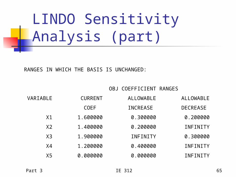
LINDO Sensitivity Analysis (part)
RANGES IN WHICH THE BASIS IS UNCHANGED:
OBJ COEFFICIENT RANGES
VARIABLE CURRENT ALLOWABLE ALLOWABLE
COEF INCREASE DECREASE
X1 1.600000 0.300000 0.200000
X2 1.400000 0.200000 INFINITY
X3 1.900000 INFINITY 0.300000
X4 1.200000 0.400000 INFINITY
X5 0.000000 0.000000 INFINITY
Part 3 IE 312 66
Interpretation As long as prices for the NE region
are between $1.4 and $1.9, we want to sell the same quantity to each region, etc.
Part 3 IE 312 67
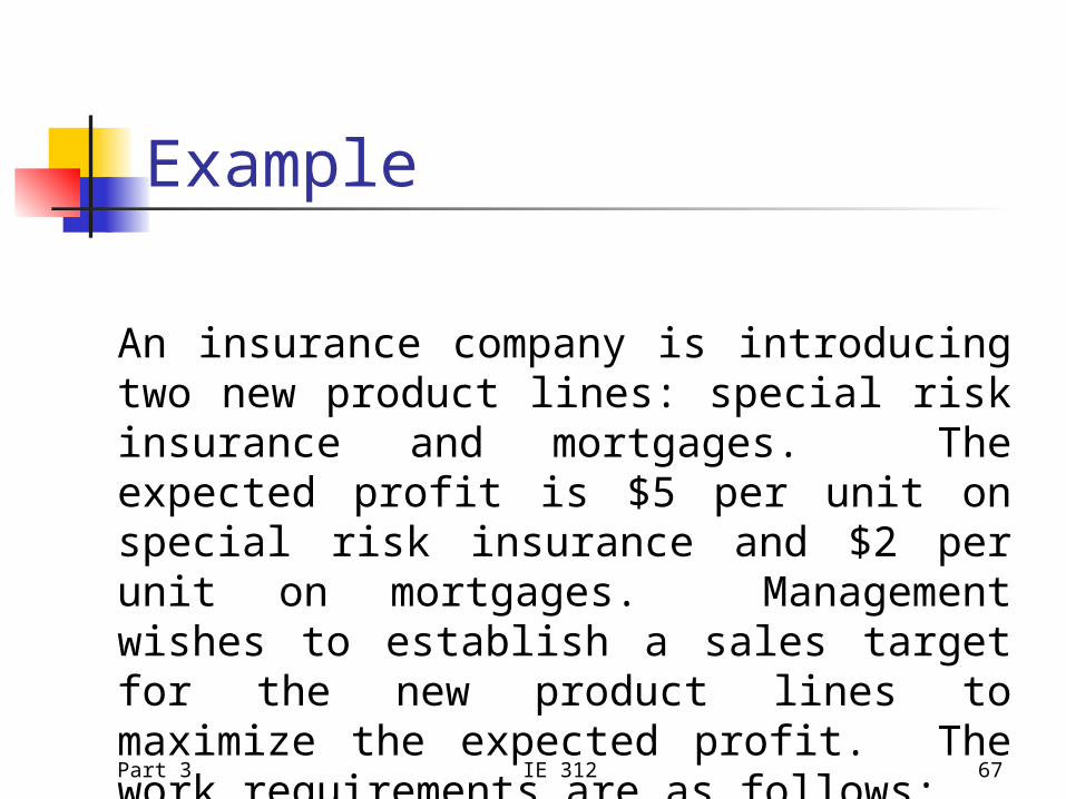
Example
An insurance company is introducing two new product lines: special risk insurance and mortgages. The expected profit is $5 per unit on special risk insurance and $2 per unit on mortgages. Management wishes to establish a sales target for the new product lines to maximize the expected profit. The work requirements are as follows:

Part 3 IE 312 68
LINDO Formulation
max 5 x1 + 2 x2
st
3 x1 + 2 x2 <= 2400x2 <= 8002 x1 <= 1200x1 >=0x2 >=0
end
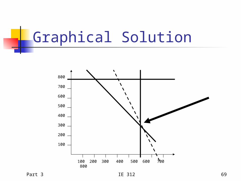
Part 3 IE 312 69
Graphical Solution
100 200 300 400 500 600 700 800
800
700
600
500
400
300
200
100

Part 3 IE 312 70
Solution
VARIABLE VALUE REDUCED COST
X1 600.000000 0.000000
X2 300.000000 0.000000
ROW SLACK OR SURPLUS DUAL PRICES
2) 0.000000 1.000000
3) 500.000000 0.000000
4) 0.000000 1.000000
5) 600.000000 0.000000
6) 300.000000 0.000000
Part 3 IE 312 71
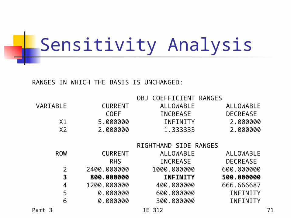
Sensitivity Analysis
RANGES IN WHICH THE BASIS IS UNCHANGED:
OBJ COEFFICIENT RANGES VARIABLE CURRENT ALLOWABLE ALLOWABLE COEF INCREASE DECREASE X1 5.000000 INFINITY 2.000000 X2 2.000000 1.333333 2.000000
RIGHTHAND SIDE RANGES ROW CURRENT ALLOWABLE ALLOWABLE RHS INCREASE DECREASE 2 2400.000000 1000.000000 600.000000 3 800.000000 INFINITY 500.000000 4 1200.000000 400.000000 666.666687 5 0.000000 600.000000 INFINITY 6 0.000000 300.000000 INFINITY
Part 3 IE 312 72
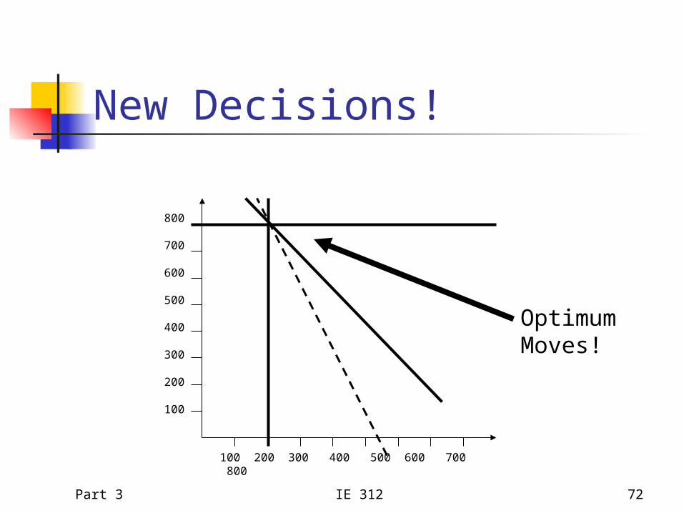
New Decisions!
100 200 300 400 500 600 700 800
800
700
600
500
400
300
200
100
OptimumMoves!
Part 3 IE 312 73
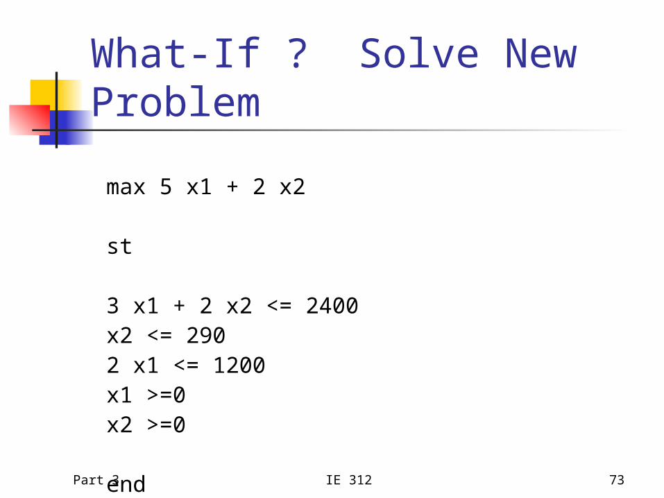
What-If ? Solve New Problem
max 5 x1 + 2 x2
st
3 x1 + 2 x2 <= 2400x2 <= 2902 x1 <= 1200x1 >=0x2 >=0
end
Part 3 IE 312 74
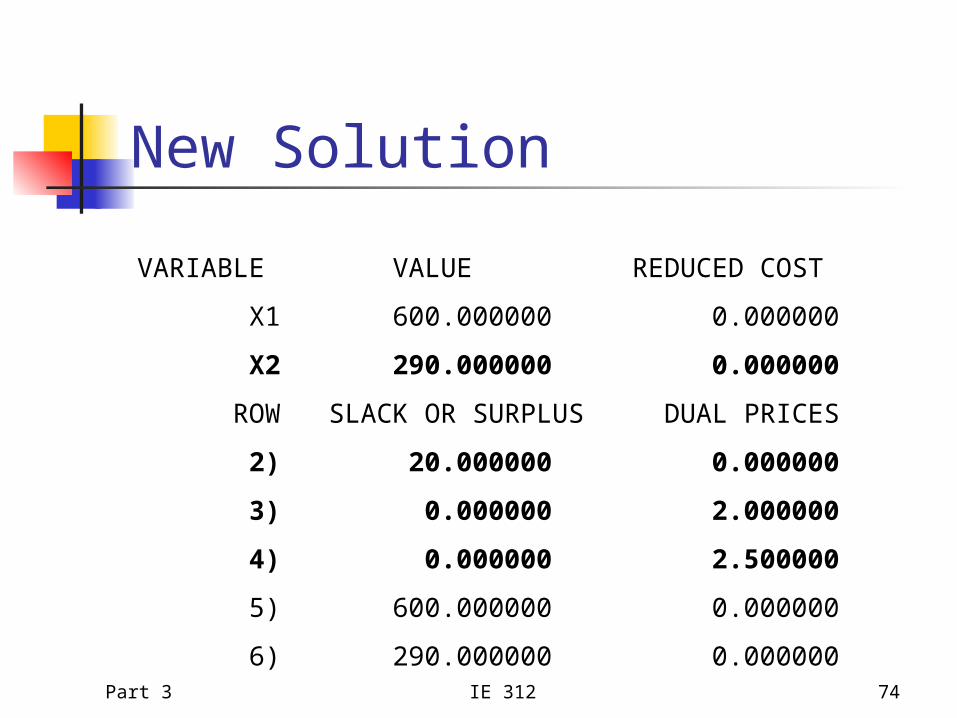
New Solution
VARIABLE VALUE REDUCED COST
X1 600.000000 0.000000
X2 290.000000 0.000000
ROW SLACK OR SURPLUS DUAL PRICES
2) 20.000000 0.000000
3) 0.000000 2.000000
4) 0.000000 2.500000
5) 600.000000 0.000000
6) 290.000000 0.000000
Part 3 IE 312 75
Interior Point Methods
Simplex always stays on the boundary
Can take short cuts across the interior
Interior point methods More effort in each move
More improvement in each move
Much faster for large problems
Part 3 IE 312 76
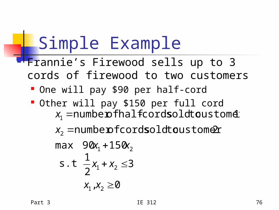
Simple Example Frannie’s Firewood sells up to 3 cords of
firewood to two customers One will pay $90 per half-cord Other will pay $150 per full cord
0,
32
1s.t
15090max
2customer tosold cords ofnumber
1customer tosold cords-half ofnumber
21
21
21
2
1
xx
xx
xx
x
x
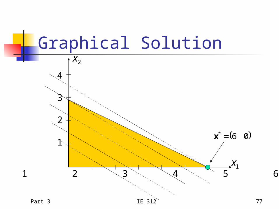
Part 3 IE 312 77
Graphical Solution
1 2 3 4 5 6
4
3
2
1
1x
2x
06* x
Part 3 IE 312 78
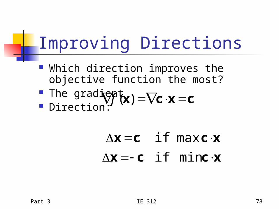
Improving Directions Which direction improves the objective
function the most? The gradient Direction:
xccx
xccx
cxcx
DD
minif
maxif
)(f
Part 3 IE 312 79
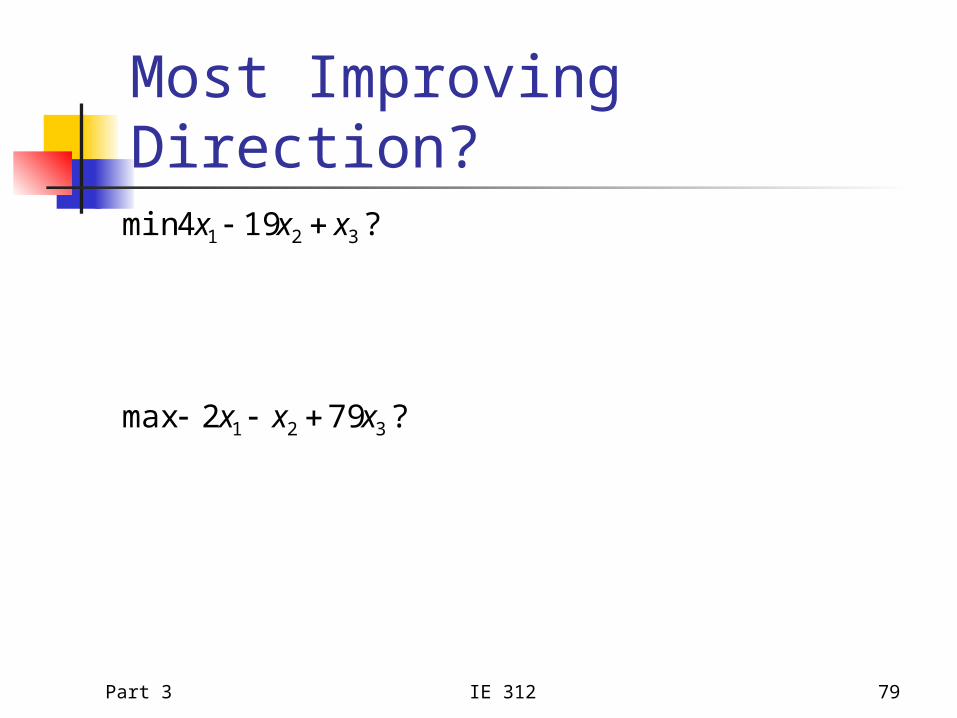
Most Improving Direction?
?792max
?194min
321
321
xxx
xxx
Part 3 IE 312 80
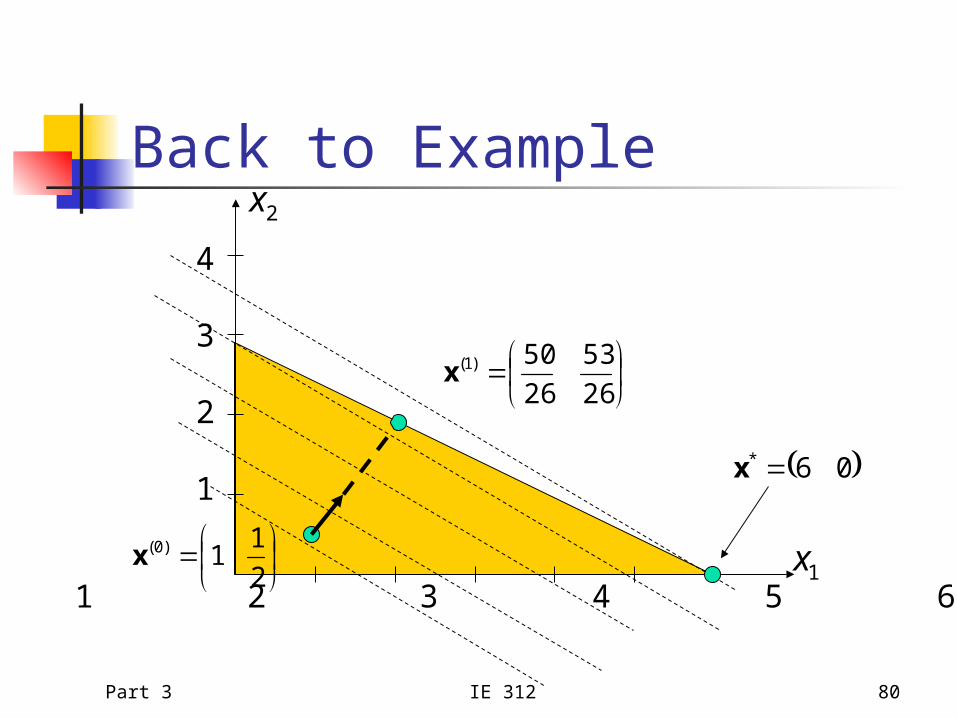
Back to Example
1 2 3 4 5 6
4
3
2
1
1x
2x
06* x
2
11)0(x
26
53
26
50)1(x
Part 3 IE 312 81
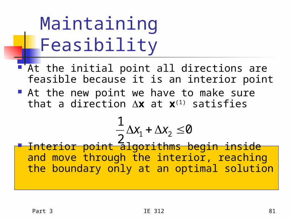
Maintaining Feasibility At the initial point all directions are
feasible because it is an interior point At the new point we have to make sure
that a direction Dx at x(1) satisfies
Interior point algorithms begin inside and move through the interior, reaching the boundary only at an optimal solution
02
121 DD xx
Part 3 IE 312 82
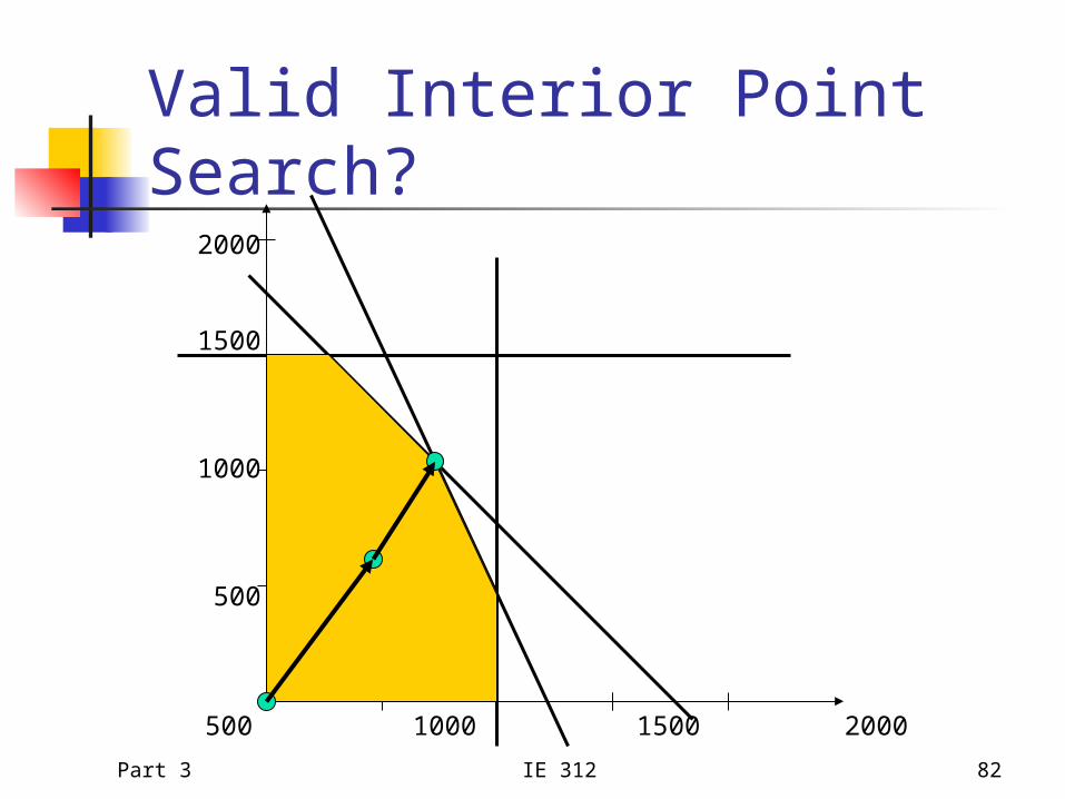
Valid Interior Point Search?2000
1500
1000
500
500 1000 1500 2000

Part 3 IE 312 83
Valid Interior Point Search?2000
1500
1000
500
500 1000 1500 2000
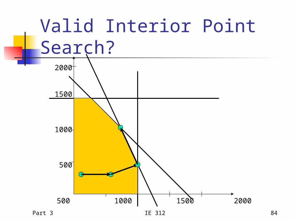
Part 3 IE 312 84
Valid Interior Point Search?2000
1500
1000
500
500 1000 1500 2000

Part 3 IE 312 85
LP Standard Form For Simplex used the form
In Frannie’s Firewood
0x
bAxxc
s.t.
maxmin/
0,,
32
1s.t
15090max
321
321
21
xxx
xxx
xx
Part 3 IE 312 86
Benefits of Standard Form?
In Simplex: Made easy to check which variables are basic,
non-basic, etc. Needed to know which solutions are on boundary
Here quite similar: Know which are not on boundary Check that nonnegativity constraints are strict!
A feasible solution to standard LP is interior point if every component is strictly positive
Part 3 IE 312 87
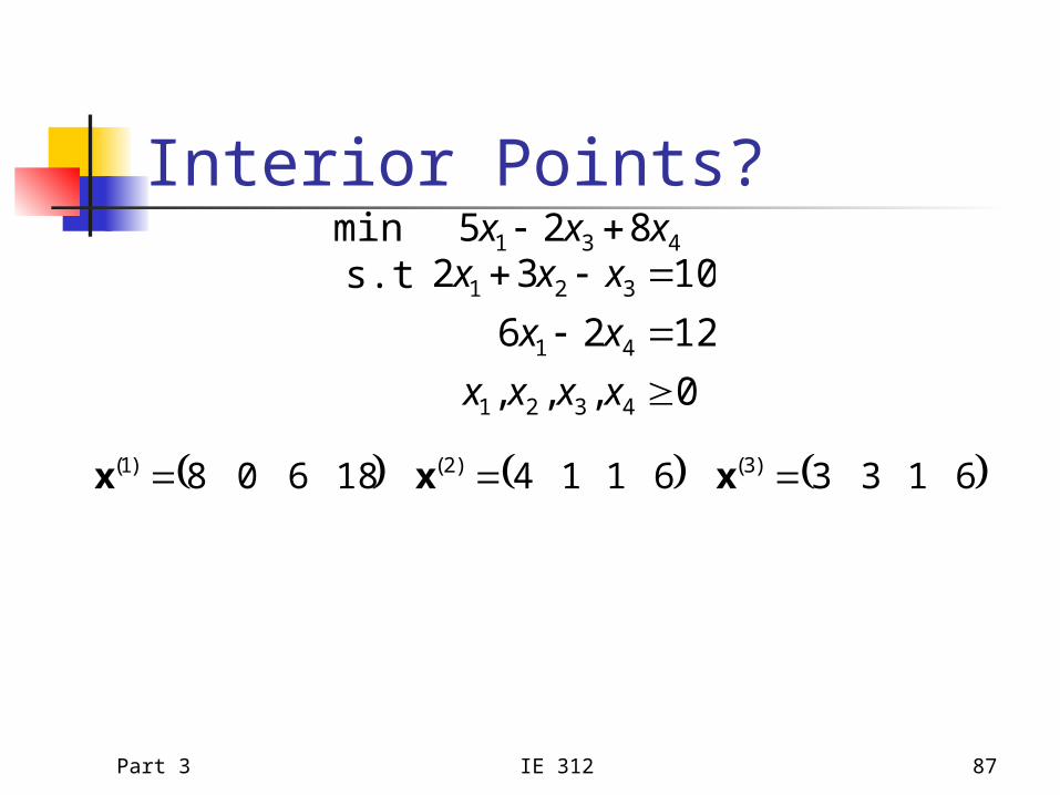
Interior Points?
0,,,
1226
1032s.t825min
4321
41
321
431
xxxx
xx
xxxxxx
6133611418608 )3()2()1( xxx
Part 3 IE 312 88
Projections Must satisfy main equality constraints
Want direction Dx that satisfies this equation and is as nearly d as possible
The projection of a vector d onto a system of equalities is the vector that satisfies the constraints and minimizes the total squared difference between the components
0xA
bAx
D
Part 3 IE 312 89
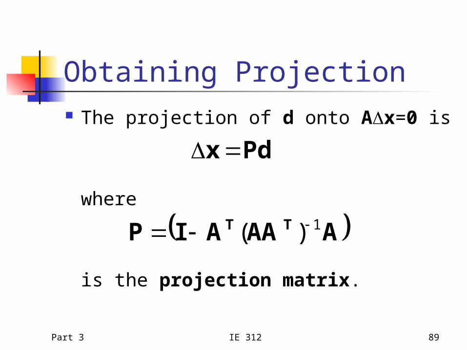
Obtaining Projection The projection of d onto ADx=0 is
where
is the projection matrix.
Pdx D
AAAAIP TT 1)(
Part 3 IE 312 90
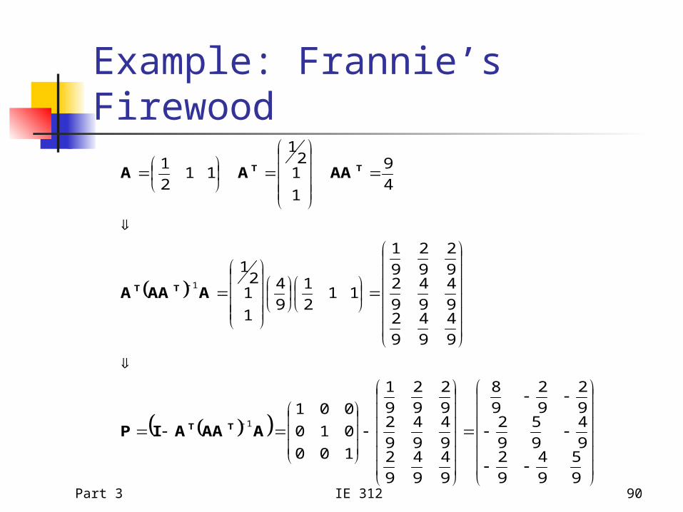
Example: Frannie’s Firewood
9
5
9
4
9
29
4
9
5
9
29
2
9
2
9
8
9
4
9
4
9
29
4
9
4
9
29
2
9
2
9
1
100
010
001
9
4
9
4
9
29
4
9
4
9
29
2
9
2
9
1
112
1
9
4
1
12
1
4
9
1
12
1
112
1
1
1
AAAAIP
AAAA
AAAA
TT
TT
TT
Part 3 IE 312 91
Example
D
9
269
199
14
0
5
3
9
5
9
4
9
29
4
9
5
9
29
2
9
2
9
8
Pdx
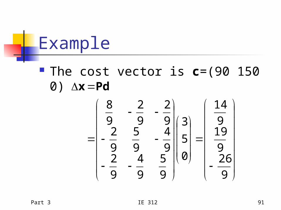
The cost vector is c=(90 150 0)
Part 3 IE 312 92
Improvement The projection matrix is design to
make an improving direction feasible with minimum changes
Is it still an improving direction? Yes!
The projection Dx=Pc of c onto Ax=b is an improving direction at every x
Part 3 IE 312 93
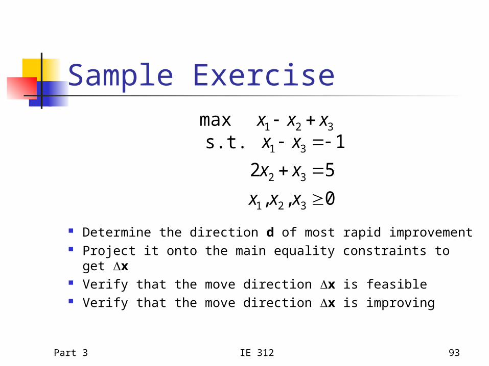
Sample Exercise
0,,
52
1s.t.max
321
32
31
321
xxx
xx
xxxxx
Determine the direction d of most rapid improvement Project it onto the main equality constraints to get Dx Verify that the move direction Dx is feasible Verify that the move direction Dx is improving

![Is there a Ghost in the [Search] Machine? Improving Search ...jason/talks/dlf2015-search-ux.pdf · Improving Search UX using Query Analysis and Machine Cues Jason A. Clark Associate](https://img.pdfslide.net/doc/110x75/603c28345fe50818960bc90d/is-there-a-ghost-in-the-search-machine-improving-search-jasontalksdlf2015-search-uxpdf.jpg)