Chapter 1

1

Chapter 1

Chapter 1: Signals and Systems ......................................................... 2

1.1 Introduction ............................................................................. 2 1.2 Signals ..................................................................................... 3

1.2.1 Sampling ........................................................................... 4 1.2.2 Discrete-Time Sinusoidal Signals ................................... 10 1.2.3 Discrete-time Exponential Signals ................................. 12 1.2.4 The Unit Impulse ............................................................ 12 1.2.5 Simple Manipulations of Discrete-Time Signals ........... 14

1.3 Systems ................................................................................. 15 Chapter 1: Problem Sheet 1

Chapter 1

2

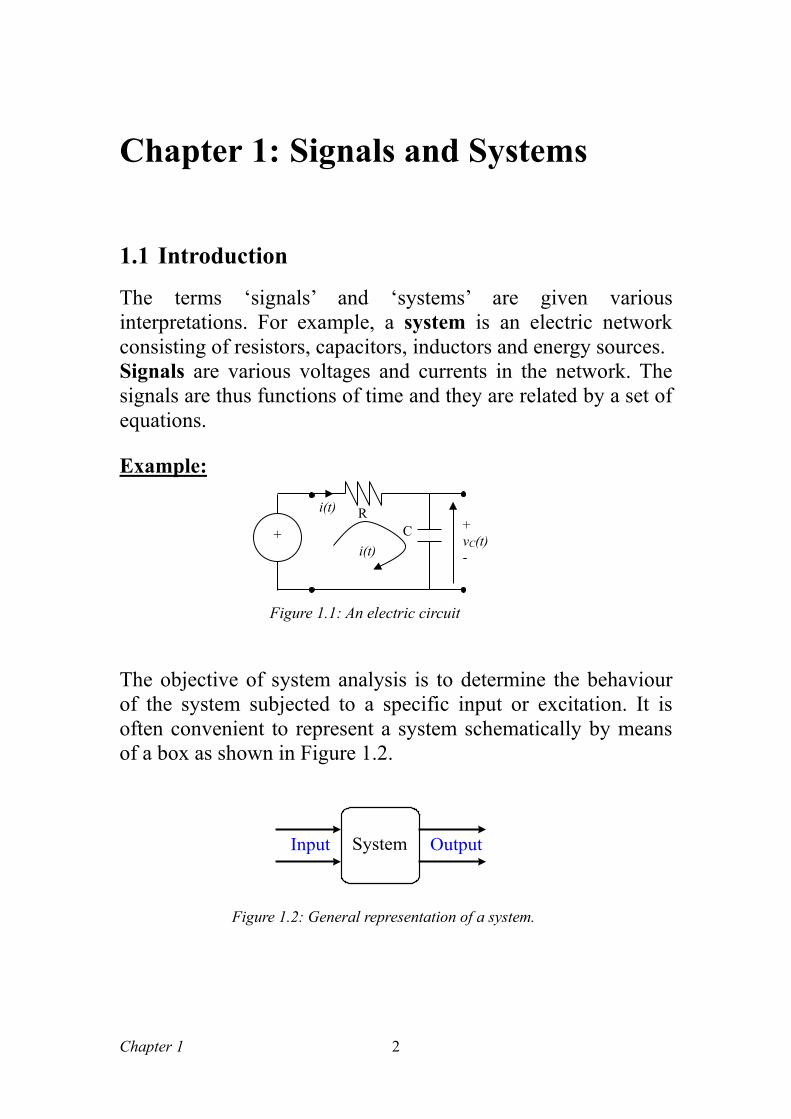
Chapter 1: Signals and Systems

1.1 Introduction The terms ‘signals’ and ‘systems’ are given various interpretations. For example, a system is an electric network consisting of resistors, capacitors, inductors and energy sources. Signals are various voltages and currents in the network. The signals are thus functions of time and they are related by a set of equations.

Example:

The objective of system analysis is to determine the behaviour of the system subjected to a specific input or excitation. It is often convenient to represent a system schematically by means of a box as shown in Figure 1.2.

Figure 1.2: General representation of a system.

i(t) R C +

vC(t) -

+ i(t)

Figure 1.1: An electric circuit

SystemInput Output

Chapter 1

3

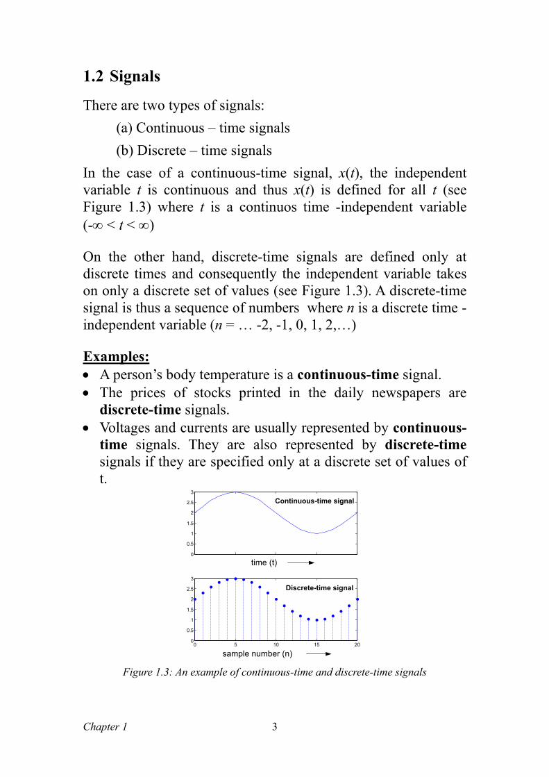
1.2 Signals There are two types of signals:

(a) Continuous – time signals (b) Discrete – time signals

In the case of a continuous-time signal, x(t), the independent variable t is continuous and thus x(t) is defined for all t (see Figure 1.3) where t is a continuos time -independent variable (-∞ < t < ∞)

On the other hand, discrete-time signals are defined only at discrete times and consequently the independent variable takes on only a discrete set of values (see Figure 1.3). A discrete-time signal is thus a sequence of numbers where n is a discrete time - independent variable (n = … -2, -1, 0, 1, 2,…)

Examples: • A person’s body temperature is a continuous-time signal. • The prices of stocks printed in the daily newspapers are

discrete-time signals. • Voltages and currents are usually represented by continuous-

time signals. They are also represented by discrete-time signals if they are specified only at a discrete set of values of t.

0

0.5

1

1.5

2

2.5

3

0 5 10 15 200

0.5

1

1.5

2

2.5

3

Continuous-time signal

Discrete-time signal

time (t)

sample number (n)

Figure 1.3: An example of continuous-time and discrete-time signals

Chapter 1

4

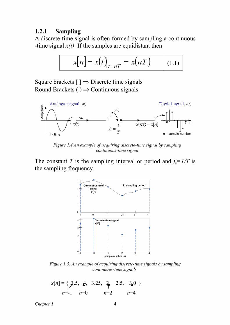
1.2.1 Sampling A discrete-time signal is often formed by sampling a continuous -time signal x(t). If the samples are equidistant then

[ ] ( ) ( )nTxtxnx nTt ===

(1.1)

Square brackets [ ] ⇒ Discrete time signals Round Brackets ( ) ⇒ Continuous signals

n0 1 7t

t - time n – sample number

Ampl

itude

, x(t) , x(n)

The constant T is the sampling interval or period and fs=1/T is the sampling frequency.

4

3

2

1

0 -T 0 T 2T 3T 4T

x(t)

-1 0 1 2 3 4

x[n]4

3

2

1

0

sample number (n)

T: sampling periodContinuous-time signal

Discrete-time signal

Figure 1.5: An example of acquiring discrete-time signals by sampling continuous-time signals.

x[n] = { 3.5, 4, 3.25, 2, 2.5, 3.0 }

n=-1 n=0 n=2 n=4

Figure 1.4 An example of acquiring discrete-time signal by sampling continuous-time signal

Chapter 1

5

It is important to recognize that x[n] is only defined for integer values of n. It is not correct to think of x[n] as being zero for n not an integer, say n=1.5. x[n] is simply undefined for non-integer values of n.

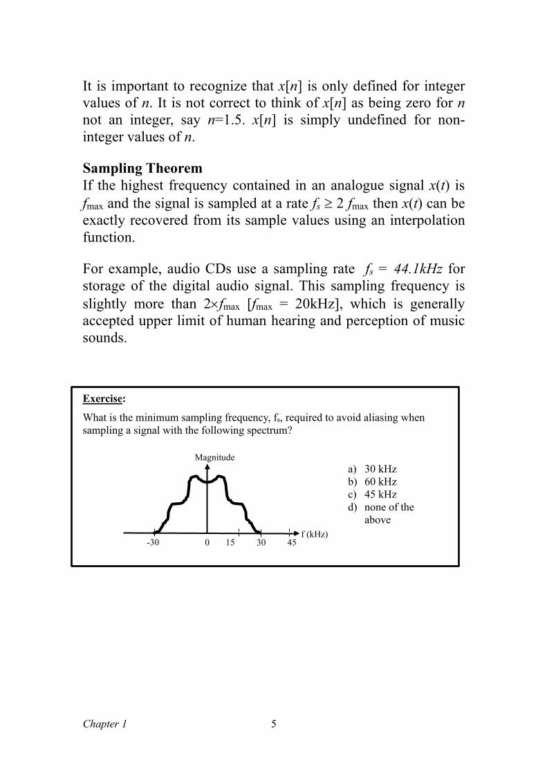
Sampling Theorem If the highest frequency contained in an analogue signal x(t) is fmax and the signal is sampled at a rate fs ≥ 2 fmax then x(t) can be exactly recovered from its sample values using an interpolation function.

For example, audio CDs use a sampling rate fs = 44.1kHz for storage of the digital audio signal. This sampling frequency is slightly more than 2×fmax [fmax = 20kHz], which is generally accepted upper limit of human hearing and perception of music sounds.

Exercise:

What is the minimum sampling frequency, fs, required to avoid aliasing when sampling a signal with the following spectrum?

30 15 45 f (kHz)

0 -30

Magnitude a) 30 kHz b) 60 kHz c) 45 kHz d) none of the

above

Chapter 1

6

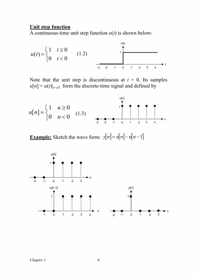
Unit step function A continuous-time unit step function u(t) is shown below:

Note that the unit step is discontinuous at t = 0. Its samples u[n] = u(t)|t=nT form the discrete-time signal and defined by

Example: Sketch the wave form: [ ] [ ] [ ]1−−= nununy

(1.2)

(1.3)

<≥

=0001

)(tt

tu

<≥

=0001

][nn

nu

Chapter 1

7

6. An analog signal x(t) = 14sin(5000πt) is sampled at a rate of 6 KHz. The resulting digital signal, x[n], is given by: a) sin[2π n] b) 14sin[ n]

c) 14sin[1000πn] d) 14sin[11000πn]

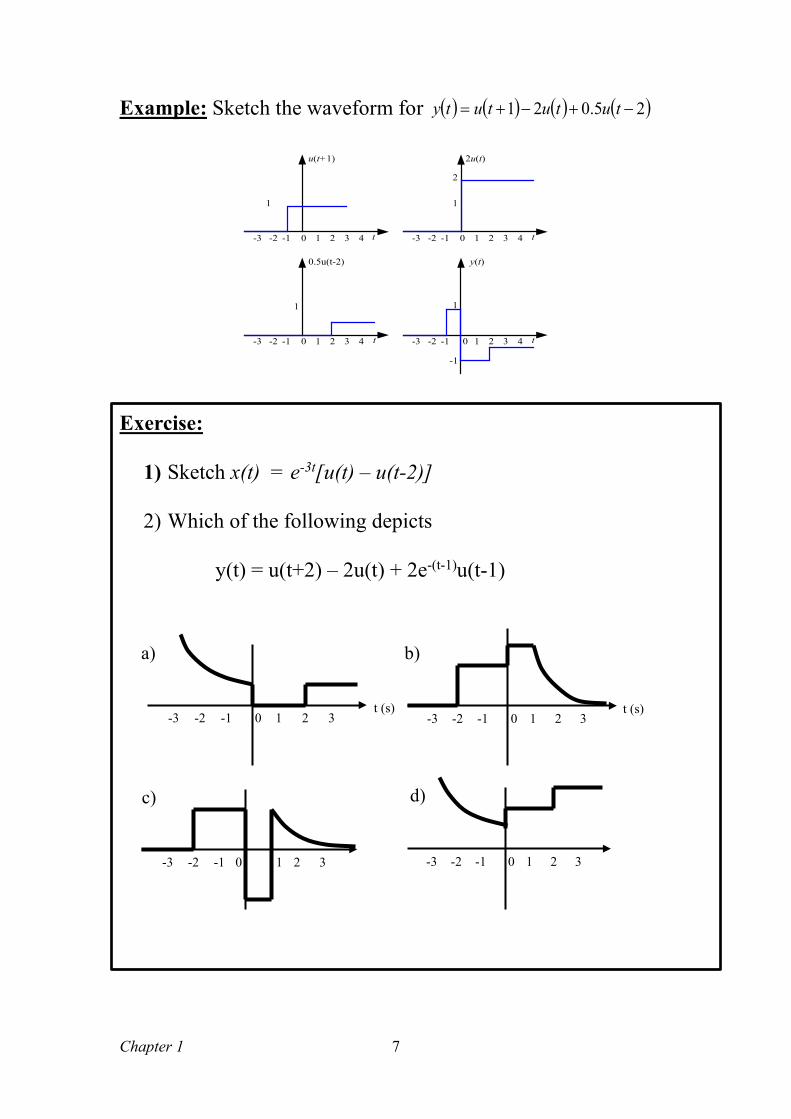
Example: Sketch the waveform for ( ) ( ) ( ) ( )25.021 −+−+= tutututy

0 1 2 3 4-1-2-3

1

t

u(t+1)

0 1 2 3 4-1-2-3

1

t

2u(t)

2

0 1 2 3 4-1-2-3

1

t

0.5u(t-2)

0 1 2 3 4-1-2-3

1

y(t)

t

-1

Exercise:

1) Sketch x(t) = e-3t[u(t) – u(t-2)]

2) Which of the following depicts

y(t) = u(t+2) – 2u(t) + 2e-(t-1)u(t-1)

0 t (s)

1 2 3 -1 -2 -3 0 t (s)

1 2 3 -1 -2 -3

0 1 2 3 -1 -2 -3 0 1 2 3 -1 -2 -3

a) b)

c) d)

Chapter 1

8

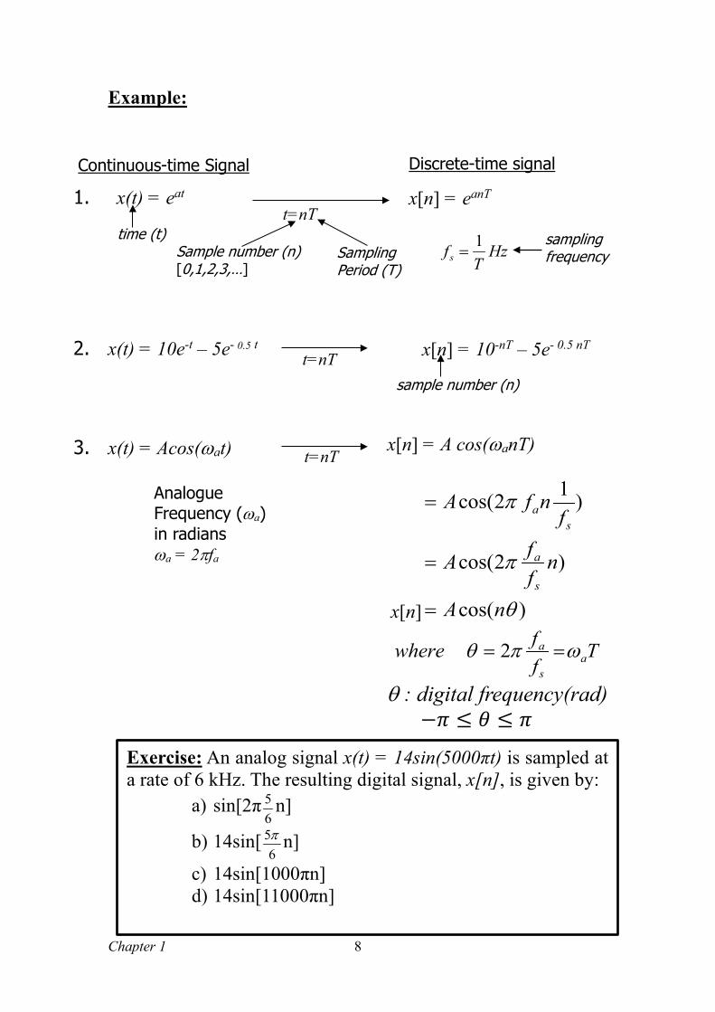
Example:

Continuous-time Signal

x[n] = eanT

Discrete-time signal

t=nT

Sample number (n) [0,1,2,3,…]

Sampling Period (T)

2. x(t) = 10e-t – 5e- 0.5 t t=nT

t=nT x[n] = A cos(ωanT)

x[n] = 10-nT – 5e- 0.5 nT

sample number (n)

3. x(t) = Acos(ωat)

Analogue Frequency (ωa) in radians ωa = 2πfa

θ : digital frequency(rad) −𝜋𝜋 ≤ 𝜃𝜃 ≤ 𝜋𝜋

1. x(t) = eat

time (t)

x[n]

HzT

fs1

=sampling frequency

)cos(

)2cos(

)12cos(

θ

π

π

nA

nffA

fnfA

s

a

sa

=

=

=

Tffwhere a

s

a ωπθ == 2

Exercise: An analog signal x(t) = 14sin(5000πt) is sampled at a rate of 6 kHz. The resulting digital signal, x[n], is given by:

a) sin[2π65 n]

b) 14sin[6

5π n]

c) 14sin[1000πn] d) 14sin[11000πn]

Chapter 1

9

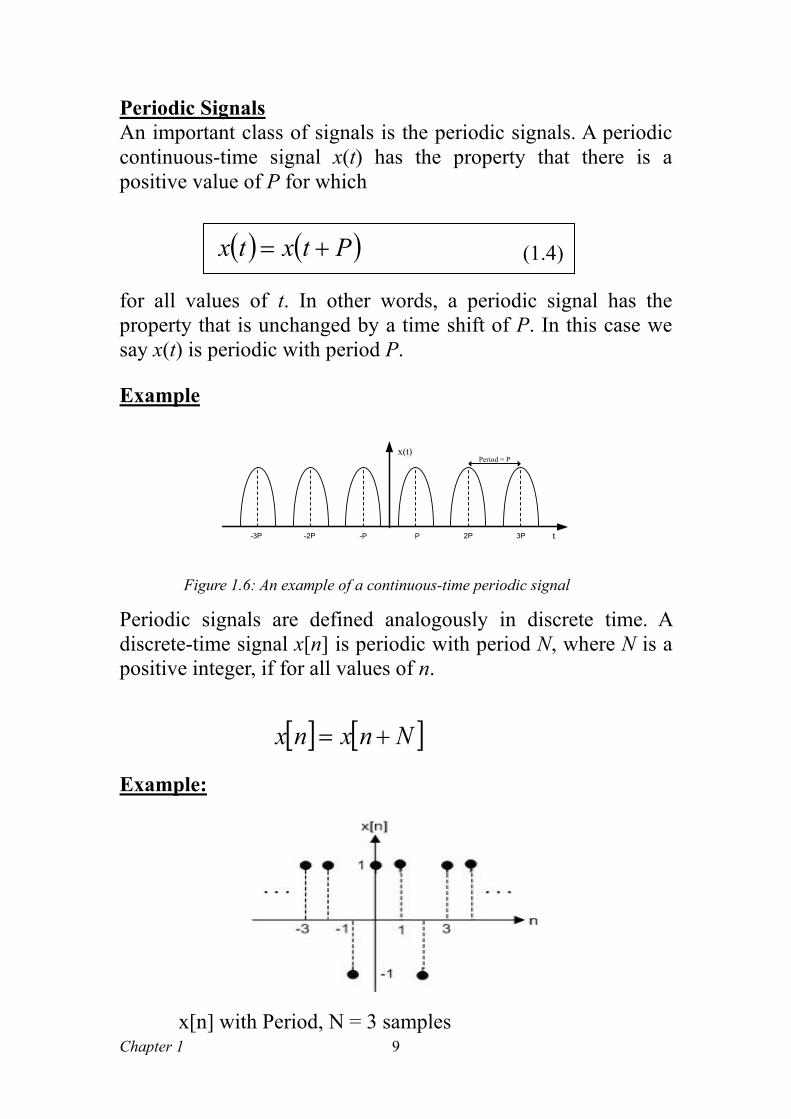
Periodic Signals An important class of signals is the periodic signals. A periodic continuous-time signal x(t) has the property that there is a positive value of P for which

for all values of t. In other words, a periodic signal has the property that is unchanged by a time shift of P. In this case we say x(t) is periodic with period P.

Example

P 2P 3P-P-2P-3P

x(t)Period = P

t

Periodic signals are defined analogously in discrete time. A discrete-time signal x[n] is periodic with period N, where N is a positive integer, if for all values of n.

Example:

Figure 1.6: An example of a continuous-time periodic signal

( ) ( )Ptxtx += (1.4)

[ ] [ ]Nnxnx +=

x[n] with Period, N = 3 samples

Chapter 1

10

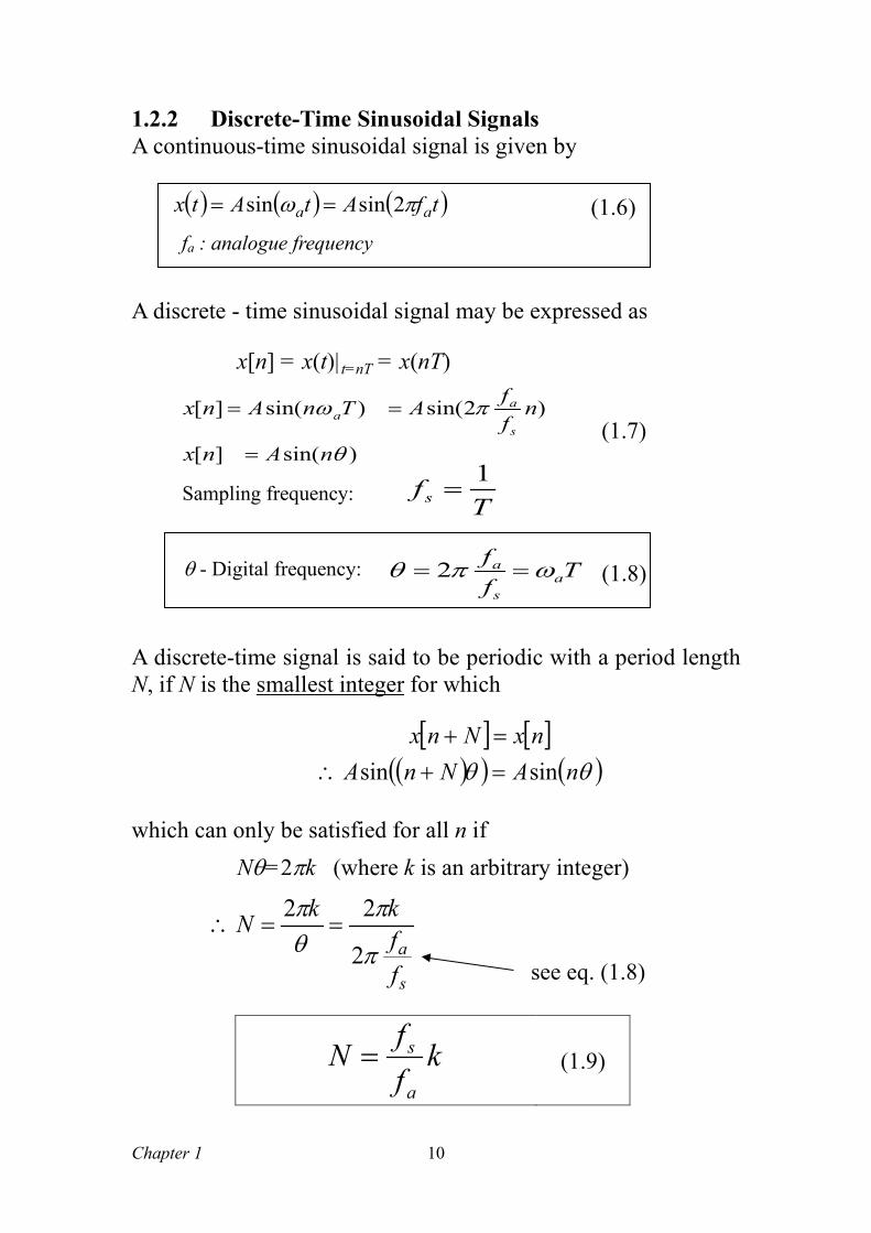
1.2.2 Discrete-Time Sinusoidal Signals A continuous-time sinusoidal signal is given by

A discrete - time sinusoidal signal may be expressed as

x[n] = x(t)|t=nT = x(nT)

A discrete-time signal is said to be periodic with a period length N, if N is the smallest integer for which

[ ] [ ]( )( ) ( )θθ nANnA

nxNnxsinsin =+∴

=+

which can only be satisfied for all n if

Nθ=2πk (where k is an arbitrary integer)

kffN

a

s=

(1.9)

( ) ( ) ( )tfAtAtx aa πω 2sinsin == (1.6)

fa : analogue frequency

(1.7)

see eq. (1.8)

(1.8)

Sampling frequency:

)sin(][

)2sin()sin(][

θ

πω

nAnx

nffATnAnx

s

aa

=

==

s

affkkN

π

πθπ

2

22==∴

T

fs1

=

θ - Digital frequency: Tff

as

a ωπθ == 2

Chapter 1

11

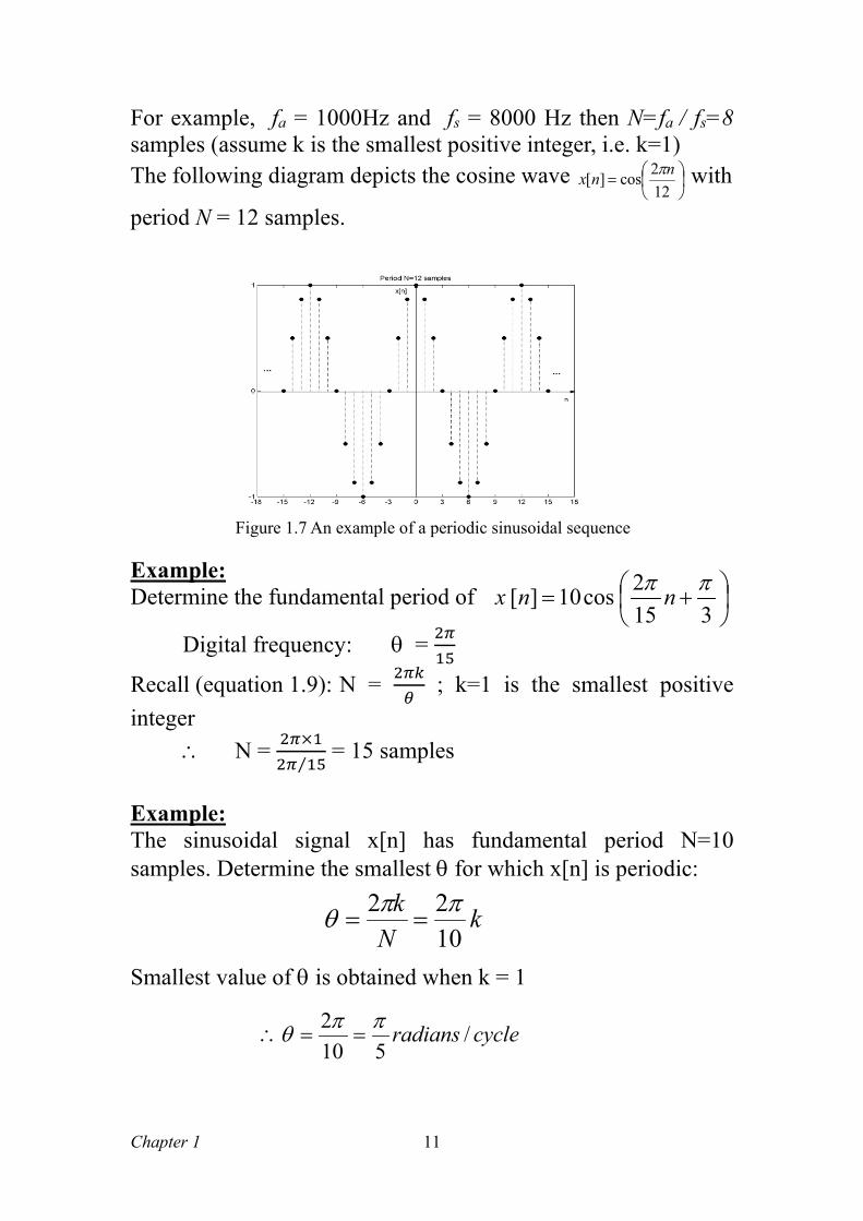
For example, fa = 1000Hz and fs = 8000 Hz then N=fa / fs=8 samples (assume k is the smallest positive integer, i.e. k=1) The following diagram depicts the cosine wave

=

122cos][ nnx π with

period N = 12 samples.

Example: Determine the fundamental period of

Digital frequency: θ = 2𝜋𝜋15

Recall (equation 1.9): N = 2𝜋𝜋𝜋𝜋𝜃𝜃

; k=1 is the smallest positive integer

∴ N = 2𝜋𝜋×12𝜋𝜋 15⁄

= 15 samples Example: The sinusoidal signal x[n] has fundamental period N=10 samples. Determine the smallest θ for which x[n] is periodic: Smallest value of θ is obtained when k = 1

kN

k1022 ππθ ==

cycleradians /510

2 ππθ ==∴

Figure 1.7 An example of a periodic sinusoidal sequence

+=

3152cos10][ ππ nnx

Chapter 1

12

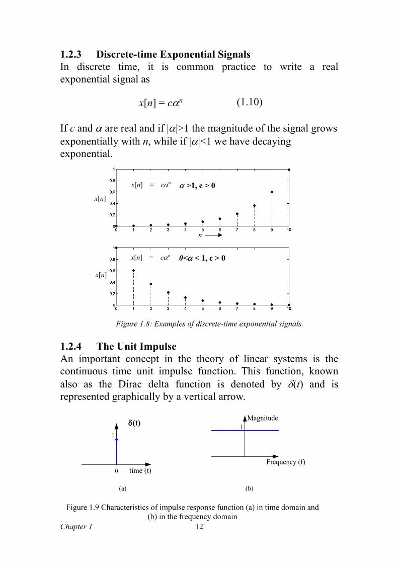
1.2.3 Discrete-time Exponential Signals In discrete time, it is common practice to write a real exponential signal as

x[n] = cαn

If c and α are real and if |α|>1 the magnitude of the signal grows exponentially with n, while if |α|<1 we have decaying exponential.

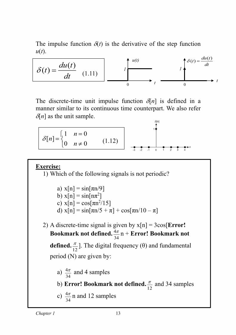
1.2.4 The Unit Impulse An important concept in the theory of linear systems is the continuous time unit impulse function. This function, known also as the Dirac delta function is denoted by δ(t) and is represented graphically by a vertical arrow.

Figure 1.8: Examples of discrete-time exponential signals.

(1.10)

α >1, c > 0 x[n] = cαn

0<α < 1, c > 0 x[n] = cαn

x[n]

x[n]

n

Figure 1.9 Characteristics of impulse response function (a) in time domain and (b) in the frequency domain

1

Frequency (f)

Magnitude

1

time (t)0

δ(t)

(a) (b)

Chapter 1

13

The impulse function δ(t) is the derivative of the step function u(t).

The discrete-time unit impulse function δ[n] is defined in a manner similar to its continuous time counterpart. We also refer δ[n] as the unit sample.

Exercise:

1) Which of the following signals is not periodic?

a) x[n] = sin[πn/9] b) x[n] = sin[nπ2] c) x[n] = cos[πn2/15] d) x[n] = sin[πn/5 + π] + cos[πn/10 – π]

2) A discrete-time signal is given by x[n] = 3cos[Error!

Bookmark not defined.344π n + Error! Bookmark not

defined.12π ]. The digital frequency (θ) and fundamental

period (N) are given by:

a) 344π and 4 samples

b) Error! Bookmark not defined.12π and 34 samples

c) 344π n and 12 samples

dttdut )()( =δ (1.11)

≠=

=0001

][nn

nδ (1.12)

0 0

1

u(t)

t

dttdut )()( =δ

1

t

Chapter 1

14

d) 172π and 17 samples

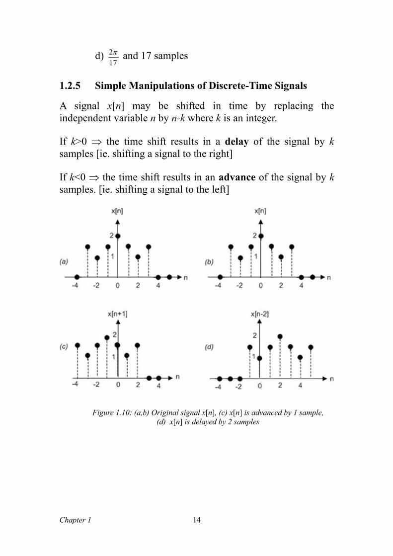
1.2.5 Simple Manipulations of Discrete-Time Signals A signal x[n] may be shifted in time by replacing the independent variable n by n-k where k is an integer.

If k>0 ⇒ the time shift results in a delay of the signal by k samples [ie. shifting a signal to the right]

If k<0 ⇒ the time shift results in an advance of the signal by k samples. [ie. shifting a signal to the left]

Figure 1.10: (a,b) Original signal x[n], (c) x[n] is advanced by 1 sample, (d) x[n] is delayed by 2 samples

Chapter 1

15

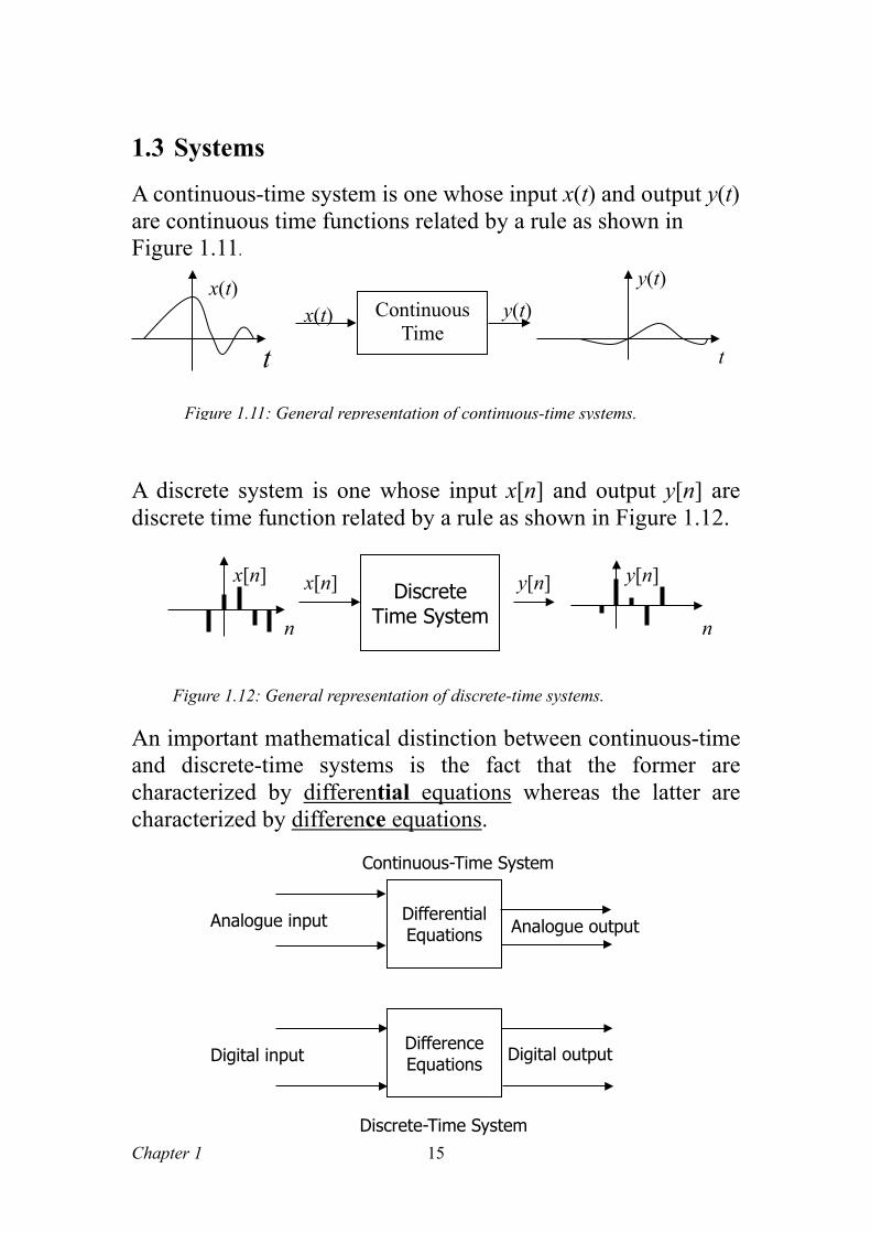
1.3 Systems A continuous-time system is one whose input x(t) and output y(t) are continuous time functions related by a rule as shown in Figure 1.11.

A discrete system is one whose input x[n] and output y[n] are discrete time function related by a rule as shown in Figure 1.12.

An important mathematical distinction between continuous-time and discrete-time systems is the fact that the former are characterized by differential equations whereas the latter are characterized by difference equations.

Figure 1.11: General representation of continuous-time systems.

Continuous Time

y(t) y(t)

t

x(t)

t

x(t)

Discrete Time System

x[n] x[n]

n

y[n]

n

y[n]

Figure 1.12: General representation of discrete-time systems.

Differential Equations

Continuous-Time System

Analogue input Analogue output

Difference Equations

Discrete-Time System

Digital input Digital output

Chapter 1

16

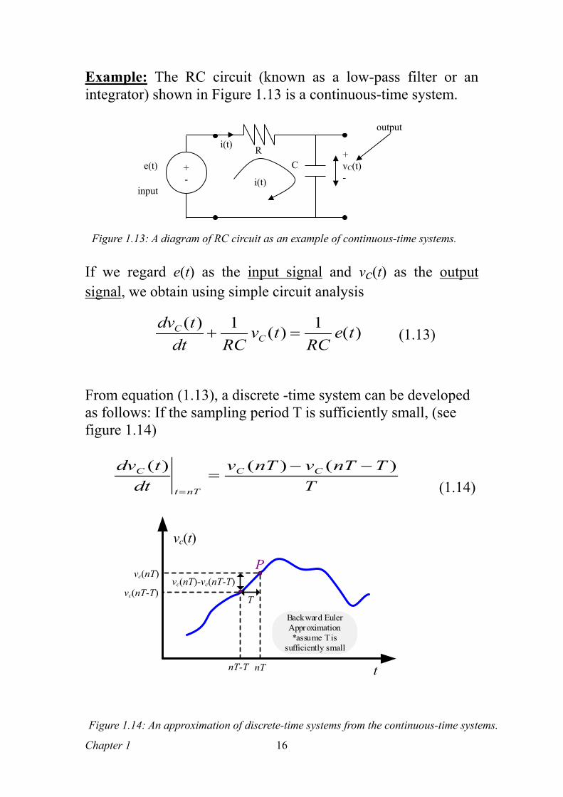
Example: The RC circuit (known as a low-pass filter or an integrator) shown in Figure 1.13 is a continuous-time system.

If we regard e(t) as the input signal and vc(t) as the output signal, we obtain using simple circuit analysis

(1.13)

From equation (1.13), a discrete -time system can be developed as follows: If the sampling period T is sufficiently small, (see figure 1.14)

TTnTvnTv

dttdv CC

nTt

C )()()( −−=

= (1.14)

i(t) R C

+ vC(t) -

+ - i(t)

e(t)

input

output

Figure 1.13: A diagram of RC circuit as an example of continuous-time systems.

Figure 1.14: An approximation of discrete-time systems from the continuous-time systems.

)(1)(1)( teRC

tvRCdt

tdvC

C =+

T

nTnT-T

vc(nT)-vc(nT-T)

vc(t)

t

vc(nT)

vc(nT-T)

P

Backward Euler Approximation *assume T is

sufficiently small

Chapter 1

17

By substituting equation (1.14) into (1.13) and replacing t by nT, we obtain:

The difference equation is:

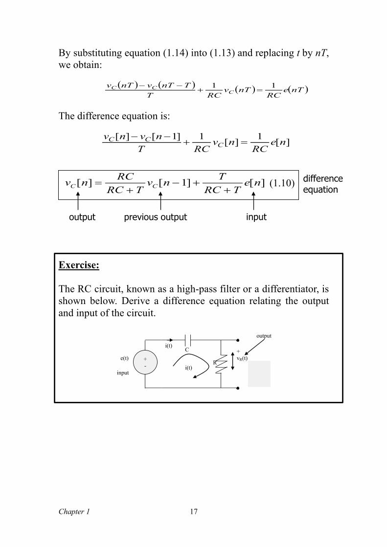
Exercise: The RC circuit, known as a high-pass filter or a differentiator, is shown below. Derive a difference equation relating the output and input of the circuit.

i(t)

R

C + vR(t)

+ - i(t)

e(t)

input

output

(1.10)

][1][1]1[][ neRC

nvRCT

nvnvC

CC =+−−

( ) ( ) ( ) ( )nTeRC

nTvRCT

TnTvnTvC

CC 11=+

−−

difference equation

][]1[][ neTRC

TnvTRC

RCnv CC ++−

+=

output previous output input

Chapter 1

18

CHAPTER 1: PROBLEM SHEET 1

Q1. Sketch the following: a) x(t) = u(t-3) – u(t-5)

b) y[n] = u[n+3] – u[n-10]

c) x(t) = e2tu(-t)

d) y[n] = u[-n]

e) h[n] = 2δ[n+1] + 2δ[n-1]

f) h[n] = u[n], p[n] = h[-n]; q[n] = h[-1-n], r[n] = h[1-n]

Q2.

a) Consider a discrete-time sequence

Determine the fundamental period of x[n]. Ans: 16 samples

b) i) Consider the sinusoidal signal

x(t) = 10 sin(2πfat) where fa -analogue frequency and t- time, Write an equation for the discrete time signal x[n]. Ans: x[n]=10 sin(nθ)

ii) If fa = 200 Hz and sampling frequency, fs = 8000 Hz, determine the fundamental

period of x[n]. Ans: N=40

End of Chapter 1

+=

58cos][ ππnnx