Part II Estimation - Econometrics Laboratory, UC Berkeley · P1: JYD/... CB495-08Drv CB495/Train KEY BOARDED March 24, 2009 22:7 Char Count= 0 Part II Estimation 183

P1: JYD/...

CB495-08Drv CB495/Train KEY BOARDED March 24, 2009 22:7 Char Count= 0

Part II

Estimation

183

P1: JYD/...


184

P1: JYD/...


8 Numerical Maximization

8.1 Motivation

Most estimation involves maximization of some function, such as thelikelihood function, the simulated likelihood function, or squared mo-ment conditions. This chapter describes numerical procedures that areused to maximize a likelihood function. Analogous procedures applywhen maximizing other functions.

Knowing and being able to apply these procedures is critical in our newage of discrete choice modeling. In the past, researchers adapted theirspecifications to the few convenient models that were available. Thesemodels were included in commercially available estimation packages,so that the researcher could estimate the models without knowing thedetails of how the estimation was actually performed from a numericalperspective. The thrust of the wave of discrete choice methods is to freethe researcher to specify models that are tailor-made to her situationand issues. Exercising this freedom means that the researcher will oftenfind herself specifying a model that is not exactly the same as any incommercial software. The researcher will need to write special code forher special model.

The purpose of this chapter is to assist in this exercise. Though notusually taught in econometrics courses, the procedures for maximiza-tion are fairly straightforward and easy to implement. Once learned, thefreedom they allow is invaluable.

8.2 Notation

The log-likelihood function takes the form LL(β) = ∑Nn=1 ln Pn(β)/N ,

where Pn(β) is the probability of the observed outcome for decisionmaker n, N is the sample size, and β is a K × 1 vector of parameters.In this chapter, we divide the log-likelihood function by N , so that LLis the average log-likelihood in the sample. Doing so does not affect thelocation of the maximum (since N is fixed for a given sample) and yet

185

P1: JYD/...


186 Estimation

LL(β)

β

βt β^

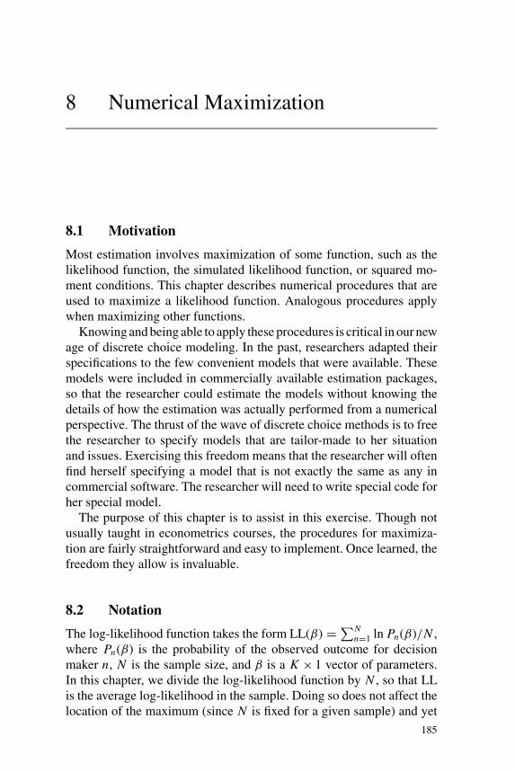
Figure 8.1. Maximum likelihood estimate.

facilitates interpretation of some of the procedures. All the proceduresoperate the same whether or not the log-likelihood is divided by N . Thereader can verify this fact as we go along by observing that N cancelsout of the relevant formulas.

The goal is to find the value of β that maximizes LL(β). In terms ofFigure 8.1, the goal is to locate β̂. Note in this figure that LL is alwaysnegative, since the likelihood is a probability between 0 and 1 and the logof any number between 0 and 1 is negative. Numerically, the maximumcan be found by “walking up” the likelihood function until no furtherincrease can be found. The researcher specifies starting values β0. Eachiteration, or step, moves to a new value of the parameters at which LL(β)is higher than at the previous value. Denote the current value of β as βt ,which is attained after t steps from the starting values. The question is:what is the best step we can take next, that is, what is the best value forβt+1?

The gradient at βt is the vector of first derivatives of LL(β) evaluatedat βt :

gt =(

∂LL(β)

∂β

)βt

.

This vector tells us which way to step in order to go up the likelihoodfunction. The Hessian is the matrix of second derivatives:

Ht =(

∂gt

∂β ′

)βt

=(

∂2LL(β)

∂β ∂β ′

)βt

.

The gradient has dimension K × 1, and the Hessian is K × K . As wewill see, the Hessian can help us to know how far to step, given that thegradient tells us in which direction to step.

P1: JYD/...


Numerical Maximization 187

8.3 Algorithms

Of the numerous maximization algorithms that have been developed overthe years, I next describe only the most prominent, with an emphasis onthe pedagogical value of the procedures as well as their practical use.Readers who are induced to explore further will find the treatments byJudge et al. (1985, Appendix B) and Ruud (2000) rewarding.

8.3.1. Newton–Raphson

To determine the best value of βt+1, take a second-order Taylor’sapproximation of LL(βt+1) around LL(βt ):

(8.1)

LL(βt+1) = LL(βt ) + (βt+1 − βt )′gt + 1

2(βt+1 − βt )

′ Ht (βt+1 − βt ).

Now find the value of βt+1 that maximizes this approximation toLL(βt+1):

∂LL(βt+1)

∂βt+1

= gt + Ht (βt+1 − βt ) = 0,

Ht (βt+1 − βt ) = −gt ,

βt+1 − βt = −H−1t gt ,

βt+1 = βt + (−H−1t )gt .

The Newton–Raphson (NR) procedure uses this formula. The stepfrom the current value of β to the new value is (−H−1

t )gt , that is,the gradient vector premultiplied by the negative of the inverse of theHessian.

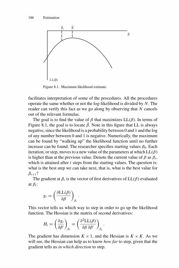
This formula is intuitively meaningful. Consider K = 1, as illustratedin Figure 8.2. The slope of the log-likelihood function is gt . The secondderivative is the Hessian Ht , which is negative for this graph, since thecurve is drawn to be concave. The negative of this negative Hessian ispositive and represents the degree of curvature. That is, −Ht is the posi-tive curvature. Each step of β is the slope of the log-likelihood functiondivided by its curvature. If the slope is positive, β is raised as in the firstpanel, and if the slope if negative, β is lowered as in the second panel. Thecurvature determines how large a step is made. If the curvature is great,meaning that the slope changes quickly as in the first panel of Figure 8.3,then the maximum is likely to be close, and so a small step is taken.

P1: JYD/...


188 Estimation

LL(β)

β

βt

β

βt

Positive slope move forward

LL(β)

Negative slope move backward

Figure 8.2. Direction of step follows the slope.

LL(β)

β

βt

β

Greater curvature

smaller step

LL(β)

β^

βt

Less curvature

larger step

β^

Figure 8.3. Step size is inversely related to curvature.

(Dividing the gradient by a large number gives a small number.) Con-versely, if the curvature is small, meaning that the slope is not changingmuch, then the maximum seems to be further away and so a larger step istaken.

Three issues are relevant to the NR procedure.

Quadratics

If LL(β) were exactly quadratic in β, then the NR procedurewould reach the maximum in one step from any starting value. This factcan easily be verified with K = 1. If LL(β) is quadratic, then it can bewritten as

LL(β) = a + bβ + cβ2.

The maximum is

∂LL(β)

∂β= b + 2cβ = 0,

β̂ = − b

2c.

P1: JYD/...



β

LL(β)

βt

LL(βt)LL(βt+1

)

βt+1

Actual LL

Quadratic

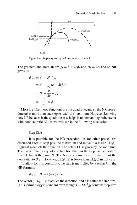
Figure 8.4. Step may go beyond maximum to lower LL.

The gradient and Hessian are gt = b + 2cβt and Ht = 2c, and so NRgives us

βt+1 = βt − H−1t gt

= βt − 1

2c(b + 2cβt )

= βt − b

2c− βt

= − b

2c= β̂.

Most log-likelihood functions are not quadratic, and so the NR proce-dure takes more than one step to reach the maximum. However, knowinghow NR behaves in the quadratic case helps in understanding its behaviorwith nonquadratic LL, as we will see in the following discussion.

Step Size

It is possible for the NR procedure, as for other proceduresdiscussed later, to step past the maximum and move to a lower LL(β).Figure 8.4 depicts the situation. The actual LL is given by the solid line.The dashed line is a quadratic function that has the slope and curvaturethat LL has at the point βt . The NR procedure moves to the top of thequadratic, to βt+1. However, LL(βt+1) is lower than LL(βt ) in this case.

To allow for this possibility, the step is multiplied by a scalar λ in theNR formula:

βt+1 = βt + λ(−Ht )−1gt .

The vector (−Ht )−1gt is called the direction, and λ is called the step size.

(This terminology is standard even though (−Ht )−1gt contains step-size

P1: JYD/...


190 Estimation

β

LL(β)

βt βt+1

for λ=1

Actual LL

Quadratic

βt+1

for λ=2

βt+1

for λ=4

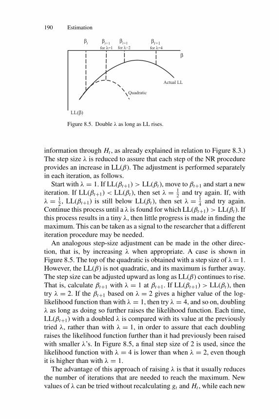
Figure 8.5. Double λ as long as LL rises.

information through Ht , as already explained in relation to Figure 8.3.)The step size λ is reduced to assure that each step of the NR procedureprovides an increase in LL(β). The adjustment is performed separatelyin each iteration, as follows.

Start with λ = 1. If LL(βt+1) > LL(βt ), move to βt+1 and start a newiteration. If LL(βt+1) < LL(βt ), then set λ = 1

2and try again. If, with

λ = 12, LL(βt+1) is still below LL(βt ), then set λ = 1

4and try again.

Continue this process until a λ is found for which LL(βt+1) > LL(βt ). Ifthis process results in a tiny λ, then little progress is made in finding themaximum. This can be taken as a signal to the researcher that a differentiteration procedure may be needed.

An analogous step-size adjustment can be made in the other direc-tion, that is, by increasing λ when appropriate. A case is shown inFigure 8.5. The top of the quadratic is obtained with a step size of λ = 1.However, the LL(β) is not quadratic, and its maximum is further away.The step size can be adjusted upward as long as LL(β) continues to rise.That is, calculate βt+1 with λ = 1 at βt+1. If LL(βt+1) > LL(βt ), thentry λ = 2. If the βt+1 based on λ = 2 gives a higher value of the log-likelihood function than with λ = 1, then try λ = 4, and so on, doublingλ as long as doing so further raises the likelihood function. Each time,LL(βt+1) with a doubled λ is compared with its value at the previouslytried λ, rather than with λ = 1, in order to assure that each doublingraises the likelihood function further than it had previously been raisedwith smaller λ’s. In Figure 8.5, a final step size of 2 is used, since thelikelihood function with λ = 4 is lower than when λ = 2, even thoughit is higher than with λ = 1.

The advantage of this approach of raising λ is that it usually reducesthe number of iterations that are needed to reach the maximum. Newvalues of λ can be tried without recalculating gt and Ht , while each new

P1: JYD/...



iteration requires calculation of these terms. Adjusting λ can thereforequicken the search for the maximum.

Concavity

If the log-likelihood function is globally concave, then the NRprocedure is guaranteed to provide an increase in the likelihood functionat each iteration. This fact is demonstrated as follows. LL(β) being con-cave means that its Hessian is negative definite at all values of β. (In onedimension, the slope of LL(β) is declining, so that the second derivativeis negative.) If H is negative definite, then H−1 is also negative definite,and −H−1 is positive definite. By definition, a symmetric matrix Mis positive definite if x ′Mx > 0 for any x �= 0. Consider a first-orderTaylor’s approximation of LL(βt+1) around LL(βt ):

LL(βt+1) = LL(βt ) + (βt+1 − βt )′gt .

Under the NR procedure, βt+1 − βt = λ(−H−1t )gt . Substituting gives

LL(βt+1) = LL(βt ) + (λ( − H−1

t

)gt

)′gt

= LL(βt ) + λg′t

( − H−1t

)gt .

Since −H−1 is positive definite, we have g′t (−H−1

t )gt > 0 andLL(βt+1) > LL(βt ). Note that since this comparison is based on a first-order approximation, an increase in LL(β) may only be obtained in asmall neighborhood of βt . That is, the value of λ that provides an in-crease might be small. However, an increase is indeed guaranteed at eachiteration if LL(β) is globally concave.

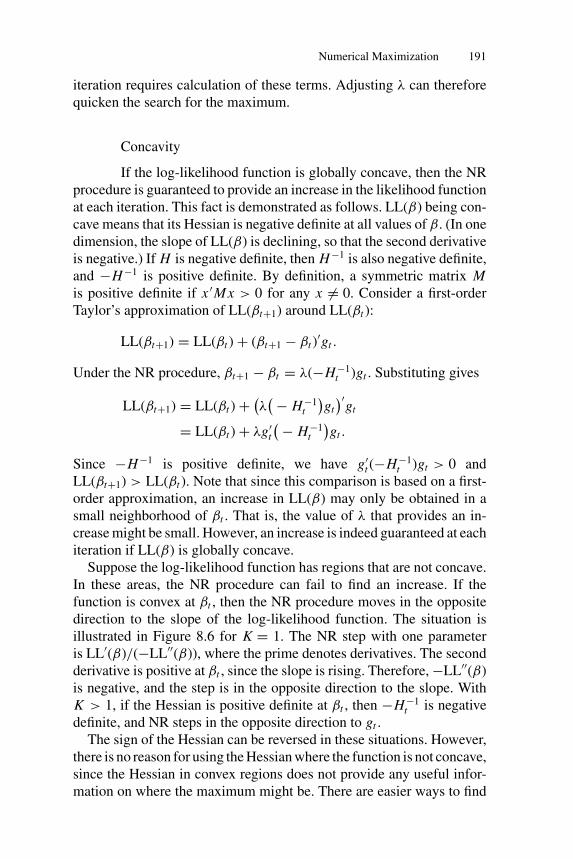
Suppose the log-likelihood function has regions that are not concave.In these areas, the NR procedure can fail to find an increase. If thefunction is convex at βt , then the NR procedure moves in the oppositedirection to the slope of the log-likelihood function. The situation isillustrated in Figure 8.6 for K = 1. The NR step with one parameteris LL′(β)/(−LL′′(β)), where the prime denotes derivatives. The secondderivative is positive at βt , since the slope is rising. Therefore, −LL′′(β)is negative, and the step is in the opposite direction to the slope. WithK > 1, if the Hessian is positive definite at βt , then −H−1

t is negativedefinite, and NR steps in the opposite direction to gt .

The sign of the Hessian can be reversed in these situations. However,there is no reason for using the Hessian where the function is not concave,since the Hessian in convex regions does not provide any useful infor-mation on where the maximum might be. There are easier ways to find

P1: JYD/...


192 Estimation

β

LL(β)

βt

Figure 8.6. NR in the convex portion of LL.

an increase in these situations than calculating the Hessian and reversingits sign. This issue is part of the motivation for other procedures.

The NR procedure has two drawbacks. First, calculation of the Hessianis usually computation-intensive. Procedures that avoid calculating theHessian at every iteration can be much faster. Second, as we have justshown, the NR procedure does not guarantee an increase in each step ifthe log-likelihood function is not globally concave. When −H−1

t is notpositive definite, an increase is not guaranteed.

Other approaches use approximations to the Hessian that address thesetwo issues. The methods differ in the form of the approximation. Eachprocedure defines a step as

βt+1 = βt + λMt gt ,

where Mt is a K × K matrix. For NR, Mt = −H−1. Other proceduresuse Mt ’s that are easier to calculate than the Hessian and are necessarilypositive definite, so as to guarantee an increase at each iteration even inconvex regions of the log-likelihood function.

8.3.2. BHHH

The NR procedure does not utilize the fact that the function be-ing maximized is actually the sum of log likelihoods over a sample ofobservations. The gradient and Hessian are calculated just as one woulddo in maximizing any function. This characteristic of NR provides gen-erality, in that the NR procedure can be used to maximize any function,not just a log likelihood. However, as we will see, maximization can befaster if we utilize the fact that the function being maximized is a sumof terms in a sample.

We need some additional notation to reflect the fact that the log-likelihood function is a sum over observations. The score of an

P1: JYD/...



observation is the derivative of that observation’s log likelihood withrespect to the parameters: sn(βt ) = ∂ ln Pn(β)/∂β evaluated at βt . Thegradient, which we defined earlier and used for the NR procedure, is theaverage score: gt = ∑

n sn(βt )/N . The outer product of observation n’sscore is the K × K matrix

sn(βt )sn(βt )′ =

⎛⎜⎜⎜⎝

s1ns1

n s1ns2

n · · · s1nsK

n

s1ns2

n s2ns2

n · · · s2nsK

n......

...s1

nsKn s2

nsKn · · · sK

n sKn

⎞⎟⎟⎟⎠ ,

where skn is the kth element of sn(βt ) with the dependence on βt

omitted for convenience. The average outer product in the sample isBt = ∑

n sn(βt )sn(βt )′/N . This average is related to the covariance ma-

trix: if the average score were zero, then B would be the covariancematrix of scores in the sample. Often Bt is called the “outer prod-uct of the gradient.” This term can be confusing, since Bt is not theouter product of gt . However, it does reflect the fact that the score isan observation-specific gradient and Bt is the average outer product ofthese observation-specific gradients.

At the parameters that maximize the likelihood function, the averagescore is indeed zero. The maximum occurs where the slope is zero,which means that the gradient, that is, the average score, is zero. Sincethe average score is zero, the outer product of the scores, Bt , becomesthe variance of the scores. That is, at the maximizing values of theparameters, Bt is the variance of scores in the sample.

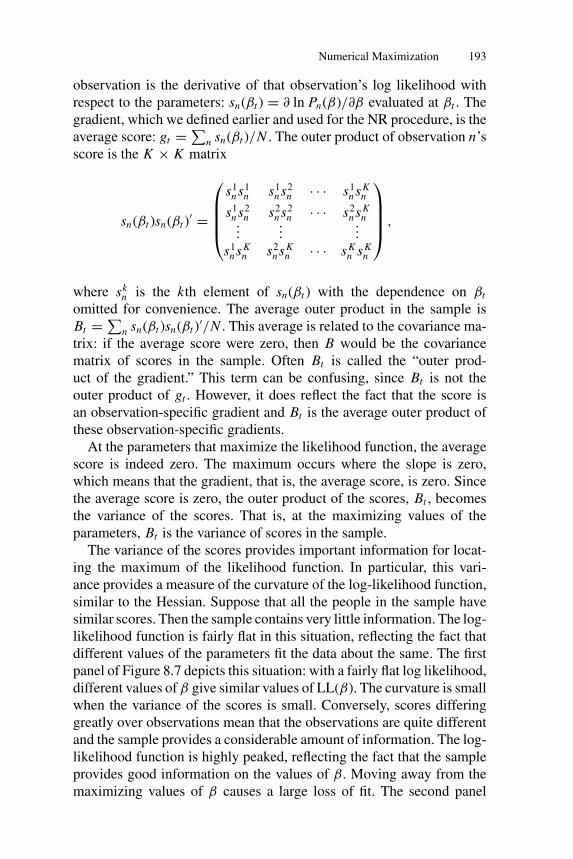
The variance of the scores provides important information for locat-ing the maximum of the likelihood function. In particular, this vari-ance provides a measure of the curvature of the log-likelihood function,similar to the Hessian. Suppose that all the people in the sample havesimilar scores. Then the sample contains very little information. The log-likelihood function is fairly flat in this situation, reflecting the fact thatdifferent values of the parameters fit the data about the same. The firstpanel of Figure 8.7 depicts this situation: with a fairly flat log likelihood,different values of β give similar values of LL(β). The curvature is smallwhen the variance of the scores is small. Conversely, scores differinggreatly over observations mean that the observations are quite differentand the sample provides a considerable amount of information. The log-likelihood function is highly peaked, reflecting the fact that the sampleprovides good information on the values of β. Moving away from themaximizing values of β causes a large loss of fit. The second panel

P1: JYD/...


194 Estimation

LL(β)

ββ

LL(β)

LL nearly flat near

maximum

LL highly curved

near maximum

Figure 8.7. Shape of log-likelihood function near maximum.

of Figure 8.7 illustrates this situation. The curvature is great when thevariance of the scores is high.

These ideas about the variance of the scores and their relation to thecurvature of the log-likelihood function are formalized in the famousinformation identity. This identity states that the covariance of the scoresat the true parameters is equal to the negative of the expected Hessian. Wedemonstrate this identity in the last section of this chapter; Theil (1971)and Ruud (2000) also provide useful and heuristic proofs. However, evenwithout proof, it makes intuitive sense that the variance of the scoresprovides information on the curvature of the log-likelihood function.

Berndt, Hall, Hall, and Hausman (1974), hereafter referred to asBHHH (and commonly pronounced B-triple H), proposed using this re-lationship in the numerical search for the maximum of the log-likelihoodfunction. In particular, the BHHH procedure uses Bt in the optimizationroutine in place of −Ht . Each iteration is defined by

βt+1 = βt + λB−1t gt .

This step is the same as for NR except that Bt is used in place of −Ht .Given the preceding discussion about the variance of the scores indicat-ing the curvature of the log-likelihood function, replacing −Ht with Bt

makes sense.There are two advantages to the BHHH procedure over NR:

1. Bt is far faster to calculate that Ht . The scores must be calcu-lated to obtain the gradient for the NR procedure anyway, andso calculating Bt as the average outer product of the scores takeshardly any extra computer time. In contrast, calculating Ht re-quires calculating the second derivatives of the log-likelihoodfunction.

2. Bt is necessarily positive definite. The BHHH procedure istherefore guaranteed to provide an increase in LL(β) in eachiteration, even in convex portions of the function. Using theproof given previously for NR when −Ht is positive definite,the BHHH step λB−1

t gt raises LL(β) for a small enough λ.

P1: JYD/...



Our discussion about the relation of the variance of the scores to thecurvature of the log-likelihood function can be stated a bit more precisely.For a correctly specified model at the true parameters, B → −H asN → ∞. This relation between the two matrices is an implication ofthe information identity, discussed at greater length in the last section.This convergence suggests that Bt can be considered an approximationto −Ht . The approximation is expected to be better as the sample sizerises. And the approximation can be expected to be better close to thetrue parameters, where the expected score is zero and the informationidentity holds, than for values of β that are farther from the true values.That is, Bt can be expected to be a better approximation close to themaximum of the LL(β) than farther from the maximum.

There are some drawbacks of BHHH. The procedure can give smallsteps that raise LL(β) very little, especially when the iterative process isfar from the maximum. This behavior can arise because Bt is not a goodapproximation to −Ht far from the true value, or because LL(β) is highlynonquadratic in the area where the problem is occurring. If the functionis highly nonquadratic, NR does not perform well, as explained earlier;since BHHH is an approximation to NR, BHHH would not perform welleven if Bt were a good approximation to −Ht .

8.3.3. BHHH-2

The BHHH procedure relies on the matrix Bt , which, as we havedescribed, captures the covariance of the scores when the average scoreis zero (i.e., at the maximizing value of β). When the iterative processis not at the maximum, the average score is not zero and Bt does notrepresent the covariance of the scores.

A variant on the BHHH procedure is obtained by subtracting out themean score before taking the outer product. For any level of the averagescore, the covariance of the scores over the sampled decision makers is

Wt =∑

n

(sn(βt ) − gt )(sn(βt ) − gt )′

N,

where the gradient gt is the average score. Wt is the covariance of thescores around their mean, and Bt is the average outer product of thescores. Wt and Bt are the same when the mean gradient is zero (i.e., atthe maximizing value of β), but differ otherwise.

The maximization procedure can use Wt instead of Bt :

βt+1 = βt + λW −1t gt .

P1: JYD/...


196 Estimation

This procedure, which I call BHHH-2, has the same advantages asBHHH. Wt is necessarily positive definite, since it is a covariance matrix,and so the procedure is guaranteed to provide an increase in LL(β) atevery iteration. Also, for a correctly specified model at the true para-meters, W → −H as N → ∞, so that Wt can be considered an approx-imation to −Ht . The information identity establishes this equivalence,as it does for B.

For β’s that are close to the maximizing value, BHHH and BHHH-2give nearly the same results. They can differ greatly at values far fromthe maximum. Experience indicates, however, that the two methods arefairly similar in that either both of them work effectively for a givenlikelihood function, or neither of them does. The main value of BHHH-2is pedagogical, to elucidate the relation between the covariance of thescores and the average outer product of the scores. This relation is criticalin the analysis of the information identity in Section 8.7.

8.3.4. Steepest Ascent

This procedure is defined by the iteration formula

βt+1 = βt + λgt .

The defining matrix for this procedure is the identity matrix I . Since I ispositive definite, the method guarantees an increase in each iteration. It iscalled “steepest ascent” because it provides the greatest possible increasein LL(β) for the distance between βt and βt+1, at least for small enoughdistance. Any other step of the same distance provides less increase. Thisfact is demonstrated as follows. Take a first-order Taylor’s expansion ofLL(βt+1) around LL(βt ): LL(βt+1) = LL(βt ) + (βt+1 − βt )gt . Maximizethis expression for LL(βt+1) subject to the Euclidian distance from βt toβt+1 being

√k. That is, maximize subject to (βt+1 − βt )

′(βt+1 − βt ) = k.The Lagrangian is

L = LL(βt ) + (βt+1 − βt )gt − 1

2λ[(βt+1 − βt )

′(βt+1 − βt ) − k],

and we have

∂L

∂βt+1

= gt − 1

λ(βt+1 − βt ) = 0,

βt+1 − βt = λgt ,

βt+1 = βt + λgt ,

which is the formula for steepest ascent.

P1: JYD/...



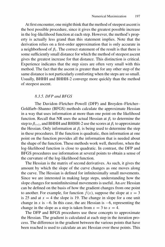
At first encounter, one might think that the method of steepest ascent isthe best possible procedure, since it gives the greatest possible increasein the log-likelihood function at each step. However, the method’s prop-erty is actually less grand than this statement implies. Note that thederivation relies on a first-order approximation that is only accurate ina neighborhood of βt . The correct statement of the result is that there issome sufficiently small distance for which the method of steepest ascentgives the greatest increase for that distance. This distinction is critical.Experience indicates that the step sizes are often very small with thismethod. The fact that the ascent is greater than for any other step of thesame distance is not particularly comforting when the steps are so small.Usually, BHHH and BHHH-2 converge more quickly than the methodof steepest ascent.

8.3.5. DFP and BFGS

The Davidon–Fletcher–Powell (DFP) and Broyden–Fletcher–Goldfarb–Shanno (BFGS) methods calculate the approximate Hessianin a way that uses information at more than one point on the likelihoodfunction. Recall that NR uses the actual Hessian at βt to determine thestep to βt+1, and BHHH and BHHH-2 use the scores at βt to approximatethe Hessian. Only information at βt is being used to determine the stepin these procedures. If the function is quadratic, then information at onepoint on the function provides all the information that is needed aboutthe shape of the function. These methods work well, therefore, when thelog-likelihood function is close to quadratic. In contrast, the DFP andBFGS procedures use information at several points to obtain a sense ofthe curvature of the log-likelihood function.

The Hessian is the matrix of second derivatives. As such, it gives theamount by which the slope of the curve changes as one moves alongthe curve. The Hessian is defined for infinitesimally small movements.Since we are interested in making large steps, understanding how theslope changes for noninfinitesimal movements is useful. An arc Hessiancan be defined on the basis of how the gradient changes from one pointto another. For example, for function f (x), suppose the slope at x = 3is 25 and at x = 4 the slope is 19. The change in slope for a one unitchange in x is −6. In this case, the arc Hessian is −6, representing thechange in the slope as a step is taken from x = 3 to x = 4.

The DFP and BFGS procedures use these concepts to approximatethe Hessian. The gradient is calculated at each step in the iteration pro-cess. The difference in the gradient between the various points that havebeen reached is used to calculate an arc Hessian over these points. This

P1: JYD/...


198 Estimation

arc Hessian reflects the change in gradient that occurs for actual move-ment on the curve, as opposed to the Hessian, which simply reflects thechange in slope for infinitesimally small steps around that point. Whenthe log-likelihood function is nonquadratic, the Hessian at any point pro-vides little information about the shape of the function. The arc Hessianprovides better information.

At each iteration, the DFP and BFGS procedures update the arcHessian using information that is obtained at the new point, that is,using the new gradient. The two procedures differ in how the updatingis performed; see Greene (2000) for details. Both methods are extremelyeffective – usually far more efficient that NR, BHHH, BHHH-2, or steep-est ascent. BFGS refines DFP, and my experience indicates that it nearlyalways works better. BFGS is the default algorithm in the optimizationroutines of many commercial software packages.

8.4 Convergence Criterion

In theory the maximum of LL(β) occurs when the gradient vector iszero. In practice, the calculated gradient vector is never exactly zero:it can be very close, but a series of calculations on a computer cannotproduce a result of exactly zero (unless, of course, the result is set tozero through a Boolean operator or by multiplication by zero, neither ofwhich arises in calculation of the gradient). The question arises: whenare we sufficiently close to the maximum to justify stopping the iterativeprocess?

The statistic mt = g′t (−H−1

t )gt is often used to evaluate convergence.The researcher specifies a small value for m, such as m̆ = 0.0001, anddetermines in each iteration whether g′

t (−H−1t )gt < m̆. If this inequality

is satisfied, the iterative process stops and the parameters at that iterationare considered the converged values, that is, the estimates. For proce-dures other than NR that use an approximate Hessian in the iterativeprocess, the approximation is used in the convergence statistic to avoidcalculating the actual Hessian. Close to the maximum, where the crite-rion becomes relevant, each form of approximate Hessian that we havediscussed is expected to be similar to the actual Hessian.

The statistic mt is the test statistic for the hypothesis that all elementsof the gradient vector are zero. The statistic is distributed chi-squaredwith K degrees of freedom. However, the convergence criterion m̆ isusually set far more stringently (that is, lower) than the critical value ofa chi-squared at standard levels of significance, so as to assure that theestimated parameters are very close to the maximizing values. Usually,the hypothesis that the gradient elements are zero cannot be rejected for a

P1: JYD/...



fairly wide area around the maximum. The distinction can be illustratedfor an estimated coefficient that has a t-statistic of 1.96. The hypothesiscannot be rejected if this coefficient has any value between zero andtwice its estimated value. However, we would not want convergence tobe defined as having reached any parameter value within this range.

It is tempting to view small changes in βt from one iteration to thenext, and correspondingly small increases in LL(βt ), as evidence thatconvergence has been achieved. However, as stated earlier, the iterativeprocedures may produce small steps because the likelihood function isnot close to a quadratic rather than because of nearing the maximum.Small changes in βt and LL(βt ) accompanied by a gradient vector thatis not close to zero indicate that the numerical routine is not effective atfinding the maximum.

Convergence is sometimes assessed on the basis of the gradient vectoritself rather than through the test statistic mt . There are two procedures:(1) determine whether each element of the gradient vector is smaller inmagnitude than some value that the researcher specifies, and (2) divideeach element of the gradient vector by the corresponding element of β,and determine whether each of these quotients is smaller in magnitudethan some value specified by the researcher. The second approach nor-malizes for the units of the parameters, which are determined by theunits of the variables that enter the model.

8.5 Local versus Global Maximum

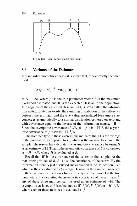
All of the methods that we have discussed are susceptible to converg-ing at a local maximum that is not the global maximum, as shown inFigure 8.8. When the log-likelihood function is globally concave, as forlogit with linear-in-parameters utility, then there is only one maximumand the issue doesn’t arise. However, most discrete choice models arenot globally concave.

A way to investigate the issue is to use a variety of starting valuesand observe whether convergence occurs at the same parameter values.For example, in Figure 8.8, starting at β0 will lead to convergenceat β1. Unless other starting values were tried, the researcher wouldmistakenly believe that the maximum of LL(β) had been achieved.Starting at β2, convergence is achieved at β̂. By comparing LL(β̂)with LL(β1), the researcher finds that β1 is not the maximizing value.Liu and Mahmassani (2000) propose a way to select starting values thatinvolves the researcher setting upper and lower bounds on each para-meter and randomly choosing values within those bounds.

P1: JYD/...


200 Estimation

β

LL(β)

β0

β^β1 β

2

Figure 8.8. Local versus global maximum.

8.6 Variance of the Estimates

In standard econometric courses, it is shown that, for a correctly specifiedmodel,

√N (β̂ − β∗)

d→ N (0, (−H)−1)

as N → ∞, where β∗ is the true parameter vector, β̂ is the maximumlikelihood estimator, and H is the expected Hessian in the population.The negative of the expected Hessian, −H, is often called the informa-tion matrix. Stated in words, the sampling distribution of the differencebetween the estimator and the true value, normalized for sample size,converges asymptotically to a normal distribution centered on zero andwith covariance equal to the inverse of the information matrix, −H−1.Since the asymptotic covariance of

√N (β̂ − β∗) is −H−1, the asymp-

totic covariance of β̂ itself is −H−1/N .The boldface type in these expressions indicates that H is the average

in the population, as opposed to H , which is the average Hessian in thesample. The researcher calculates the asymptotic covariance by using Has an estimate of H. That is, the asymptotic covariance of β̂ is calculatedas −H−1/N , where H is evaluated at β̂.

Recall that W is the covariance of the scores in the sample. At themaximizing values of β, B is also the covariance of the scores. By theinformation identity just discussed and explained in the last section, −H,which is the (negative of the) average Hessian in the sample, convergesto the covariance of the scores for a correctly specified model at the trueparameters. In calculating the asymptotic covariance of the estimates β̂,any of these three matrices can be used as an estimate of −H. Theasymptotic variance of β̂ is calculated as W −1/N , B−1/N , or −H−1/N ,where each of these matrices is evaluated at β̂.

P1: JYD/...



If the model is not correctly specified, then the asymptotic covarianceof β̂ is more complicated. In particular, for any model for which theexpected score is zero at the true parameters,

√N (β̂ − β∗)

d→ N (0, H−1VH−1),

where V is the variance of the scores in the population. When the model iscorrectly specified, the matrix −H = V by the information identity, suchthat H−1VH−1 = −H−1 and we get the formula for a correctly specifiedmodel. However, if the model is not correctly specified, this simplifica-tion does not occur. The asymptotic variance of β̂ is H−1VH−1/N . Thismatrix is called the robust covariance matrix, since it is valid whetheror not the model is correctly specified.

To estimate the robust covariance matrix, the researcher must cal-culate the Hessian H . If a procedure other than NR is being used toreach convergence, the Hessian need not be calculated at each iteration;however, it must be calculated at the final iteration. Then the asymptoticcovariance is calculated as H−1WH−1, or with B instead of W . Thisformula is sometimes called the “sandwich” estimator of the covariance,since the Hessian inverse appears on both sides.

An alternative way to estimate the covariance matrix is through boot-strapping, as suggested by Efron (1979). Under this procedure, the modelis re-estimated numerous times on different samples taken from the orig-inal sample. Let the original sample be labeled A, which consists of thedecision-makers that we have been indexing by n = 1, . . . , N . That is,the original sample consists of N observations. The estimate that isobtained on this sample is β̂. Bootstapping consists of the followingsteps:

1. Randomly sample with replacement N observations from theoriginal sample A. Since the sampling is with replacement, somedecision-makers might be represented more than once in the newsample and others might not be included at all. This new sampleis the same size as the original, but looks different from theoriginal because some decision-makers are repeated and othersare not included.

2. Re-estimate the model on this new sample, and label the estimateβr with r = 1 for this first new sample.

3. Repeated steps 1 and 2 numerous times, obtaining estimates βr

for r = 1, . . . , R where R is the number of times the estimationis repeated on a new sample.

4. Calculate the covariance of the resulting estimates around theoriginal estimate: V = 1

R

∑r (βr − β̂)(βr − β̂)′.

P1: JYD/...


202 Estimation

This V is an estimate of the asymptotic covariance matrix. The samplingvariance for any statistics that is based on the parameters is calculatedsimilarly. For scalar statistic t(β), the sampling variance is

∑r [t(βr ) −

t(β̂)]2/R.The logic of the procedure is the following. The sampling covariance

of an estimator is, by definition, a measure of the amount by which theestimates change when different samples are taken from the population.Our original sample is one sample from the population. However, if thissample is large enough, then it is probably similar to the population,such that drawing from it is similar to drawing from the populationitself. The bootstrap does just that: draws from the original sample, withreplacement, as a proxy for drawing from the population itself. Theestimates obtained on the bootstrapped samples provide information onthe distribution of estimates that would be obtained if alternative sampleshad actually been drawn from the population.

The advantage of the bootstrap is that it is conceptually straightfor-ward and does not rely on formulas that hold asymptotically but mightnot be particularly accurate for a given sample size. Its disadvantage isthat it is computer-intensive since it entails estimating the model numer-ous times. Efron and Tibshirant (1993) and Vinod (1993) provide usefuldiscussions and applications.

8.7 Information Identity

The information identity states that, for a correctly specified model atthe true parameters, V = −H, where V is the covariance matrix of thescores in the population and H is the average Hessian in the population.The score for a person is the vector of first derivatives of that person’sln P(β) with respect to the parameters, and the Hessian is the matrixof second derivatives. The information identity states that, in the popu-lation, the covariance matrix of the first derivatives equals the averagematrix of second derivatives (actually, the negative of that matrix). Thisis a startling fact, not something that would be expected or even believedif there were not proof. It has implications throughout econometrics. Theimplications that we have used in the previous sections of this chapterare easily derivable from the identity. In particular:

(1) At the maximizing value of β, W → −H as N → ∞, where Wis the sample covariance of the scores and H is the sample average ofeach observation’s Hessian. As sample size rises, the sample covarianceapproaches the population covariance: W → V. Similarly, the sampleaverage of the Hessian approaches the population average: H → H.

P1: JYD/...



Since V= −H by the information identity, W approaches the same ma-trix that −H approaches, and so they approach each other.

(2) At the maximizing value of β, B → −H as N → ∞, where B isthe sample average of the outer product of the scores. At β̂, the averagescore in the sample is zero, so that B is the same as W . The result for Wapplies for B.

We now demonstrate the information identity. We need to expand ournotation to encompass the population instead of simply the sample. LetPi (x, β) be the probability that a person who faces explanatory variablesx chooses alternative i given the parameters β. Of the people in thepopulation who face variables x , the share who choose alternative i is thisprobability calculated at the true parameters: Si (x) = Pi (x, β∗) whereβ∗ are the true parameters. Consider now the gradient of ln Pi (x, β) withrespect to β. The average gradient in the population is

(8.2) g =∫ ∑

i

∂ ln Pi (x, β)

∂βSi (x) f (x) dx,

where f (x) is the density of explanatory variables in the population.This expression can be explained as follows. The gradient for peoplewho face x and choose i is ∂ ln Pni (β)/∂β. The average gradient is theaverage of this term over all values of x and all alternatives i . The shareof people who face a given value of x is given by f (x), and the share ofpeople who face this x that choose i is Si (x). So Si (x) f (x) is the shareof the population who face x and choose i and therefore have gradient∂ ln Pi (x, β)/∂β. Summing this term over all values of i and integratingover all values of x (assuming the x’s are continuous) gives the averagegradient, as expressed in (8.2).

The average gradient in the population is equal to zero at the trueparameters. This fact can be considered either the definition of the trueparameters or the result of a correctly specified model. Also, we knowthat Si (x) = Pi (x, β∗). Substituting these facts into (8.2), we have

0 =∫ ∑

i

∂ ln Pi (x, β)

∂βPi (x, β) f (x) dx,

where all functions are evaluated at β∗. We now take the derivative ofthis equation with respect to the parameters:

0 =∫ ∑

i

(∂2 ln Pi (x, β)

∂β ∂β ′ Pi (x, β) + ∂ ln Pi (x, β)

∂β

∂ Pi (x, β)

∂β ′

)f (x) dx .

P1: JYD/...


204 Estimation

Since ∂ ln P/∂β = (1/P) ∂ P/∂β by the rules of derivatives, we cansubstitute [∂ ln Pi (x, β)/∂β ′]Pi (x, β) for ∂ Pi (x, β)/∂β ′ in the last termin parentheses:

0 =∫ ∑

i

(∂2 ln Pi (x, β)

∂β ∂β ′ Pi (x, β)

+ ∂ ln Pi (x, β)

∂β

∂lnPi (x, β)

∂β ′ Pi (x, β)

)f (x) dx .

Rearranging,

−∫ ∑

i

∂2 ln Pi (x, β)

∂β ∂β ′ Pi (x, β) f (x) dx

=∫ ∑

i

∂ ln Pi (x, β)

∂β

∂ ln Pi (x, β)

∂β ′ Pi (x, β) f (x) dx .

Since all terms are evaluated at the true parameters, we can replacePi (x, β) with Si (x) to obtain

−∫ ∑

i

∂2 ln Pi (x, β)

∂β ∂β ′ Si (x) f (x) dx

=∫ ∑

i

∂ ln Pi (x, β)

∂β

∂ ln Pi (x, β)

∂β ′ Si (x) f (x) dx .

The left-hand side is the negative of the average Hessian in the popula-tion, −H. The right-hand side is the average outer product of the gradient,which is the covariance of the gradient, V, since the average gradientis zero. Therefore, −H = V, the information identity. As stated, thematrix −H is often called the information matrix.

Documents

Part II Estimation - Econometrics Laboratory, UC Berkeley · P1: JYD/... CB495-08Drv CB495/Train KEY BOARDED March 24, 2009 22:7 Char Count= 0 Part II Estimation 183