Part III - Electrical and Computer Engineeringparhami/pres_folder/f31-book-arith-pres... · Basic Addition and Counting Carry-Lookahead Adders ... = p = ax + p(0)2 ... Performing

Apr. 2015 Computer Arithmetic, Multiplication Slide 1

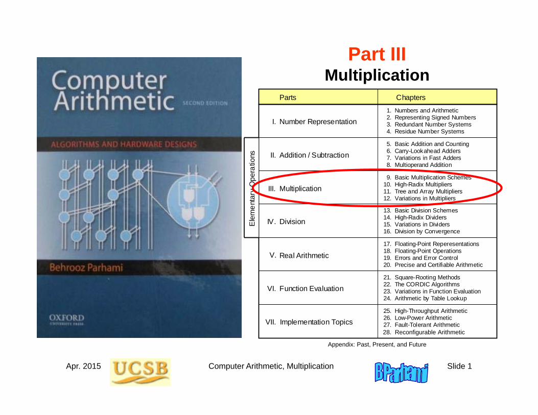
Part IIIMultiplication

Number Representation Numbers and Arithmetic Representing Signed Numbers Redundant Number Systems Residue Number Systems

Addition / Subtraction Basic Addition and Counting Carry-Lookahead Adders Variations in Fast Adders Multioperand Addition

Multiplication Basic Multiplication Schemes High-Radix Multipliers Tree and Array Multipliers Variations in Multipliers

Division Basic Division Schemes High-Radix Dividers Variations in Dividers Division by Convergence

Real Arithmetic Floating-Point Reperesentations Floating-Point Operations Errors and Error Control Precise and Certifiable Arithmetic

Function Evaluation Square-Rooting Methods The CORDIC Algorithms Variations in Function Evaluation Arithmetic by Table Lookup

Implementation Topics High-Throughput Arithmetic Low-Power Arithmetic Fault-Tolerant Arithmetic Past, Present, and Future

Parts Chapters

I.

II.

III.

IV.

V.

VI.

VII.

1. 2. 3. 4.

5. 6. 7. 8.

9. 10. 11. 12.

25. 26. 27. 28.

21. 22. 23. 24.

17. 18. 19. 20.

13. 14. 15. 16.

Ele

men

tary

Ope

ratio

ns

28. Reconfigurable Arithmetic

Appendix: Past, Present, and Future


About This Presentation

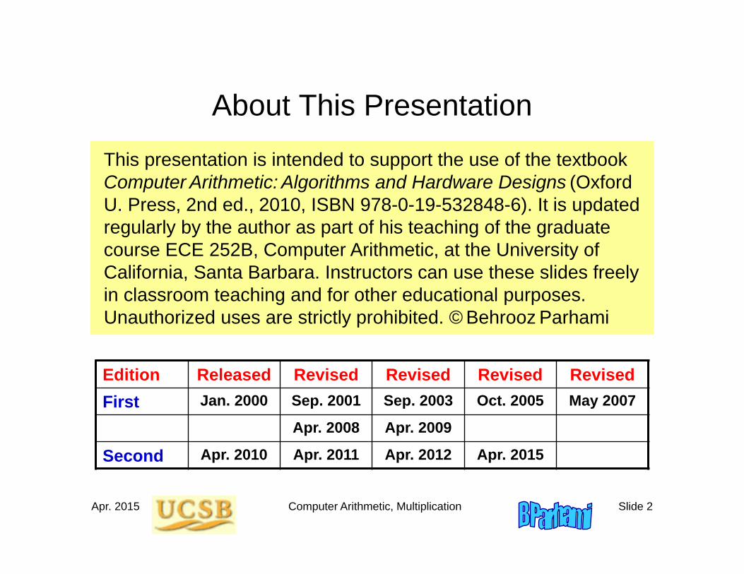
Edition Released Revised Revised Revised RevisedFirst Jan. 2000 Sep. 2001 Sep. 2003 Oct. 2005 May 2007

Apr. 2008 Apr. 2009

Second Apr. 2010 Apr. 2011 Apr. 2012 Apr. 2015

This presentation is intended to support the use of the textbook Computer Arithmetic: Algorithms and Hardware Designs (Oxford U. Press, 2nd ed., 2010, ISBN 978-0-19-532848-6). It is updated regularly by the author as part of his teaching of the graduate course ECE 252B, Computer Arithmetic, at the University of California, Santa Barbara. Instructors can use these slides freely in classroom teaching and for other educational purposes. Unauthorized uses are strictly prohibited. © Behrooz Parhami


III Multiplication

Topics in This PartChapter 9 Basic Multiplication SchemesChapter 10 High-Radix MultipliersChapter 11 Tree and Array MultipliersChapter 12 Variations in Multipliers

Review multiplication schemes and various speedup methods• Multiplication is heavily used (in arith & array indexing)• Division = reciprocation + multiplication• Multiplication speedup: high-radix, tree, recursive • Bit-serial, modular, and array multipliers


“Well, well, for a rabbit, you’re not very good at multiplying, are you?”


9 Basic Multiplication Schemes

Chapter GoalsStudy shift/add or bit-at-a-time multipliersand set the stage for faster methods andvariations to be covered in Chapters 10-12

Chapter HighlightsMultiplication = multioperand additionHardware, firmware, software algorithmsMultiplying 2’s-complement numbersThe special case of one constant operand


Basic Multiplication Schemes: Topics

Topics in This Chapter

9.1 Shift/Add Multiplication Algorithms

9.2 Programmed Multiplication

9.3 Basic Hardware Multipliers

9.4 Multiplication of Signed Numbers

9.5 Multiplication by Constants

9.6 Preview of Fast Multipliers


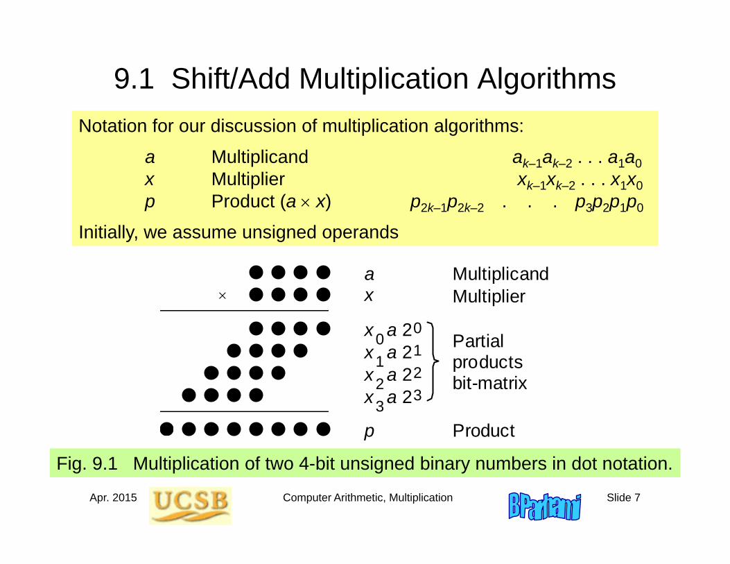
9.1 Shift/Add Multiplication AlgorithmsNotation for our discussion of multiplication algorithms:

a Multiplicand ak–1ak–2 . . . a1a0x Multiplier xk–1xk–2 . . . x1x0p Product (a x) p2k–1p2k–2 . . . p3p2p1p0

Initially, we assume unsigned operands

Fig. 9.1 Multiplication of two 4-bit unsigned binary numbers in dot notation.

Product

Partial products bit-matrix

a x

p

2

x a

0 0

1 x a 2 1 x a 2

2 2

2 3 3

x a

Multiplicand Multiplier


Preferred

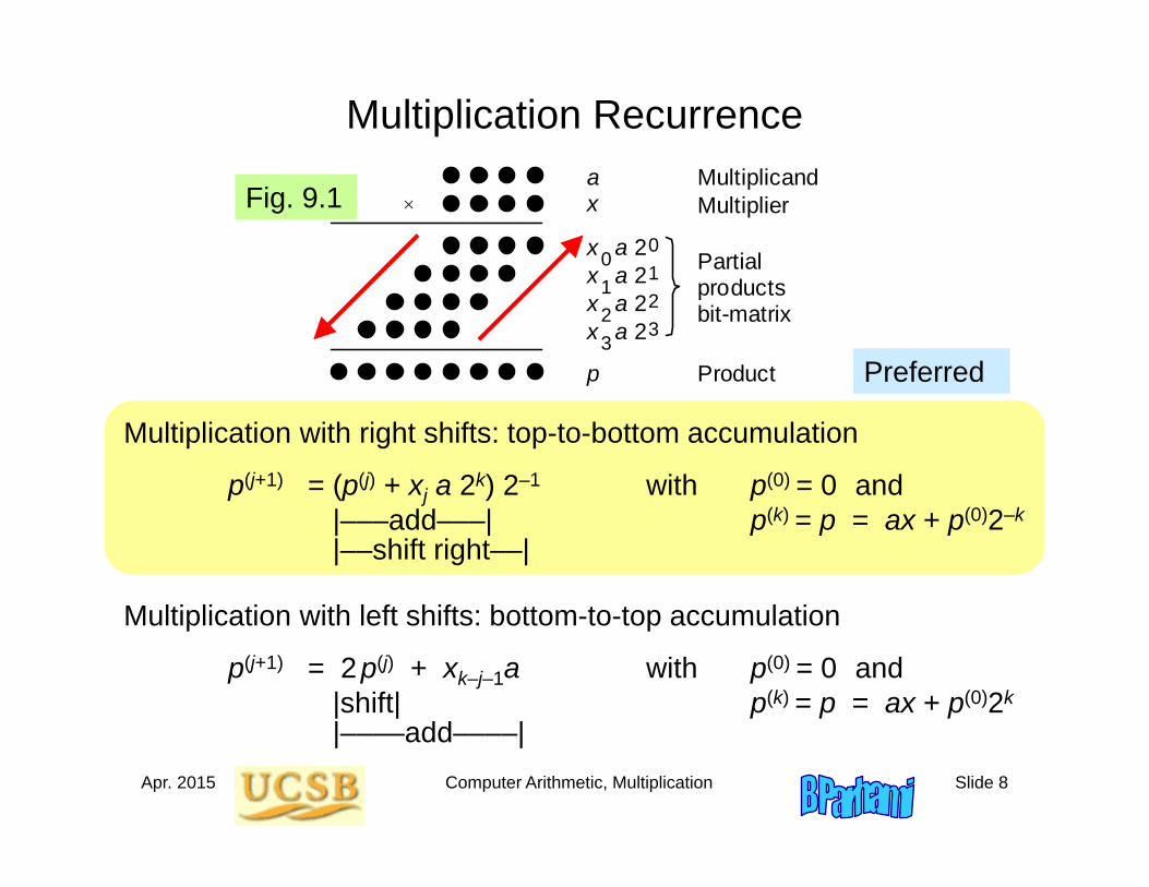
Multiplication Recurrence

Multiplication with right shifts: top-to-bottom accumulation

p(j+1) = (p(j) + xj a 2k) 2–1 with p(0) = 0 and|–––add–––| p(k) = p = ax + p(0)2–k

|––shift right––|

Product


a x

p

2

x a

0 0

1 x a 2 1 x a 2

2 2

2 3 3

x a


Multiplication with left shifts: bottom-to-top accumulation

p(j+1) = 2p(j) + xk–j–1a with p(0) = 0 and|shift| p(k) = p = ax + p(0)2k

|––––add––––|

Fig. 9.1


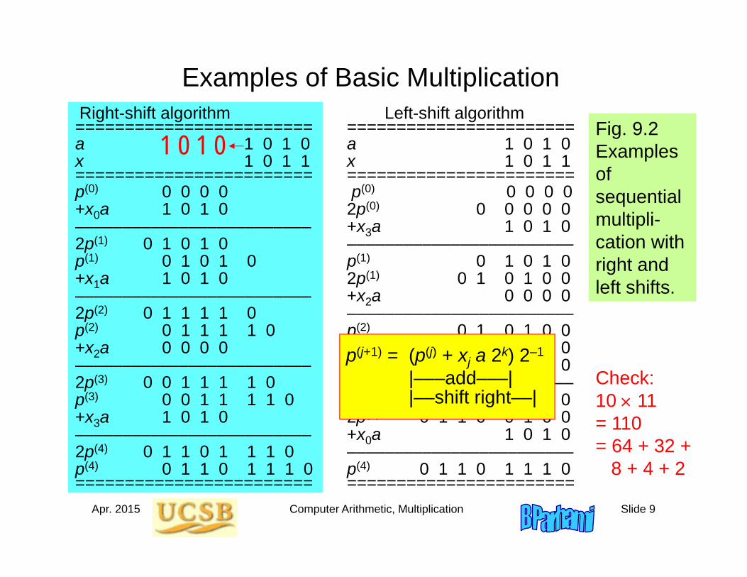
Examples of Basic Multiplication

Fig. 9.2Examples of sequential multipli-cation with right and left shifts.

Right-shift algorithm Left-shift algorithm======================== =======================a 1 0 1 0 a 1 0 1 0x 1 0 1 1 x 1 0 1 1======================== =======================p(0) 0 0 0 0 p(0) 0 0 0 0+x0a 1 0 1 0 2p(0) 0 0 0 0 0––––––––––––––––––––––––– +x3a 1 0 1 02p(1) 0 1 0 1 0 ––––––––––––––––––––––––p(1) 0 1 0 1 0 p(1) 0 1 0 1 0+x1a 1 0 1 0 2p(1) 0 1 0 1 0 0––––––––––––––––––––––––– +x2a 0 0 0 02p(2) 0 1 1 1 1 0 ––––––––––––––––––––––––p(2) 0 1 1 1 1 0 p(2) 0 1 0 1 0 0+x2a 0 0 0 0 2p(2) 0 1 0 1 0 0 0––––––––––––––––––––––––– +x1a 1 0 1 02p(3) 0 0 1 1 1 1 0 ––––––––––––––––––––––––p(3) 0 0 1 1 1 1 0 p(3) 0 1 1 0 0 1 0+x3a 1 0 1 0 2p(3) 0 1 1 0 0 1 0 0––––––––––––––––––––––––– +x0a 1 0 1 02p(4) 0 1 1 0 1 1 1 0 ––––––––––––––––––––––––p(4) 0 1 1 0 1 1 1 0 p(4) 0 1 1 0 1 1 1 0======================== =======================

p(j+1) = (p(j) + xj a 2k) 2–1

|–––add–––||––shift right––|

1 0 1 0

Check:10 11= 110= 64 + 32 +

8 + 4 + 2


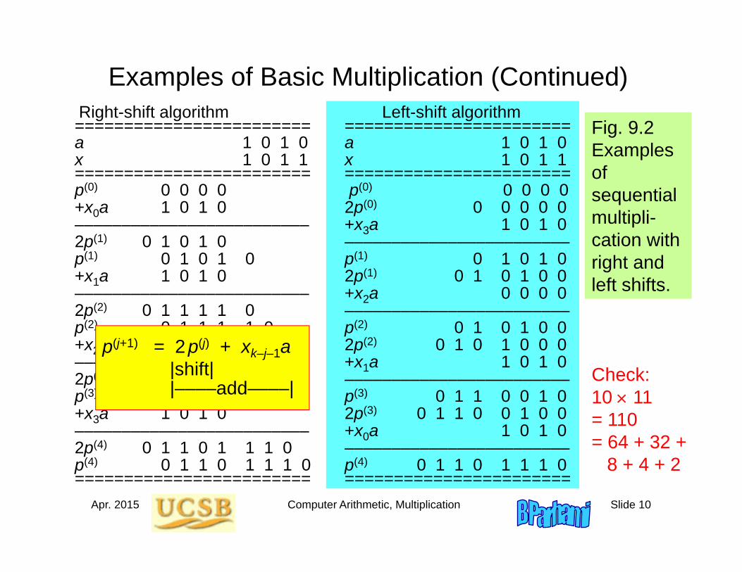
Examples of Basic Multiplication (Continued)

Fig. 9.2Examples of sequential multipli-cation with right and left shifts.

Right-shift algorithm Left-shift algorithm======================== =======================a 1 0 1 0 a 1 0 1 0x 1 0 1 1 x 1 0 1 1======================== =======================p(0) 0 0 0 0 p(0) 0 0 0 0+x0a 1 0 1 0 2p(0) 0 0 0 0 0––––––––––––––––––––––––– +x3a 1 0 1 02p(1) 0 1 0 1 0 ––––––––––––––––––––––––p(1) 0 1 0 1 0 p(1) 0 1 0 1 0+x1a 1 0 1 0 2p(1) 0 1 0 1 0 0––––––––––––––––––––––––– +x2a 0 0 0 02p(2) 0 1 1 1 1 0 ––––––––––––––––––––––––p(2) 0 1 1 1 1 0 p(2) 0 1 0 1 0 0+x2a 0 0 0 0 2p(2) 0 1 0 1 0 0 0––––––––––––––––––––––––– +x1a 1 0 1 02p(3) 0 0 1 1 1 1 0 ––––––––––––––––––––––––p(3) 0 0 1 1 1 1 0 p(3) 0 1 1 0 0 1 0+x3a 1 0 1 0 2p(3) 0 1 1 0 0 1 0 0––––––––––––––––––––––––– +x0a 1 0 1 02p(4) 0 1 1 0 1 1 1 0 ––––––––––––––––––––––––p(4) 0 1 1 0 1 1 1 0 p(4) 0 1 1 0 1 1 1 0======================== =======================

p(j+1) = 2p(j) + xk–j–1a|shift||––––add––––|

Check:10 11= 110= 64 + 32 +

8 + 4 + 2


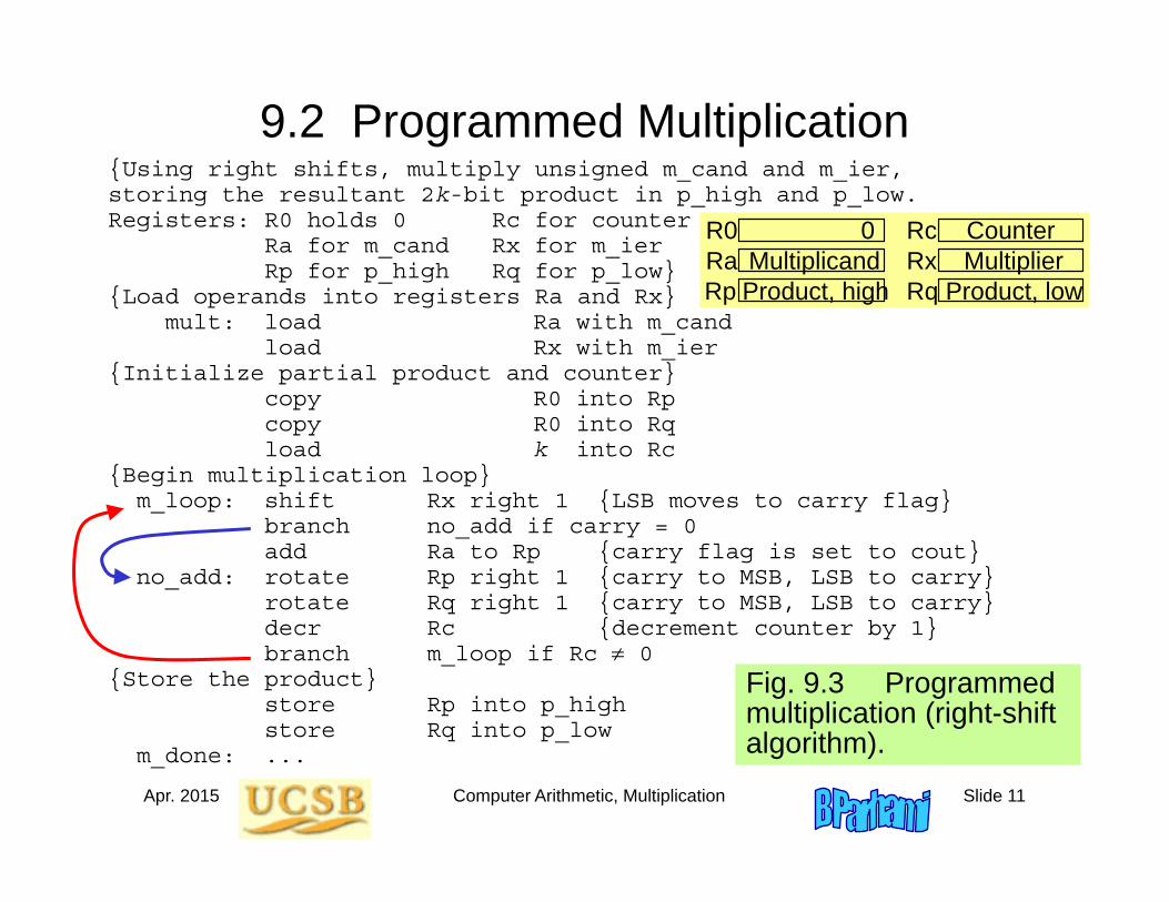
9.2 Programmed Multiplication

Fig. 9.3 Programmed multiplication (right-shift algorithm).

{Using right shifts, multiply unsigned m_cand and m_ier, storing the resultant 2k-bit product in p_high and p_low. Registers: R0 holds 0 Rc for counter

Ra for m_cand Rx for m_ierRp for p_high Rq for p_low}

{Load operands into registers Ra and Rx}mult: load Ra with m_cand

load Rx with m_ier {Initialize partial product and counter}

copy R0 into Rpcopy R0 into Rqload k into Rc

{Begin multiplication loop}m_loop: shift Rx right 1 {LSB moves to carry flag}

branch no_add if carry = 0 add Ra to Rp {carry flag is set to cout}

no_add: rotate Rp right 1 {carry to MSB, LSB to carry}rotate Rq right 1 {carry to MSB, LSB to carry}decr Rc {decrement counter by 1}branch m_loop if Rc 0

{Store the product}store Rp into p_highstore Rq into p_low

m_done: ...

R0 Rc Counter0Ra RxRp Rq

Multiplicand MultiplierProduct, high Product, low


Time Complexity of Programmed Multiplication

Assume k-bit words

k iterations of the main loop6-7 instructions per iteration, depending on the multiplier bit

Thus, 6k + 3 to 7k + 3 machine instructions,ignoring operand loads and result store

k = 32 implies 200+ instructions on average

This is too slow for many modern applications!

Microprogrammed multiply would be somewhat better


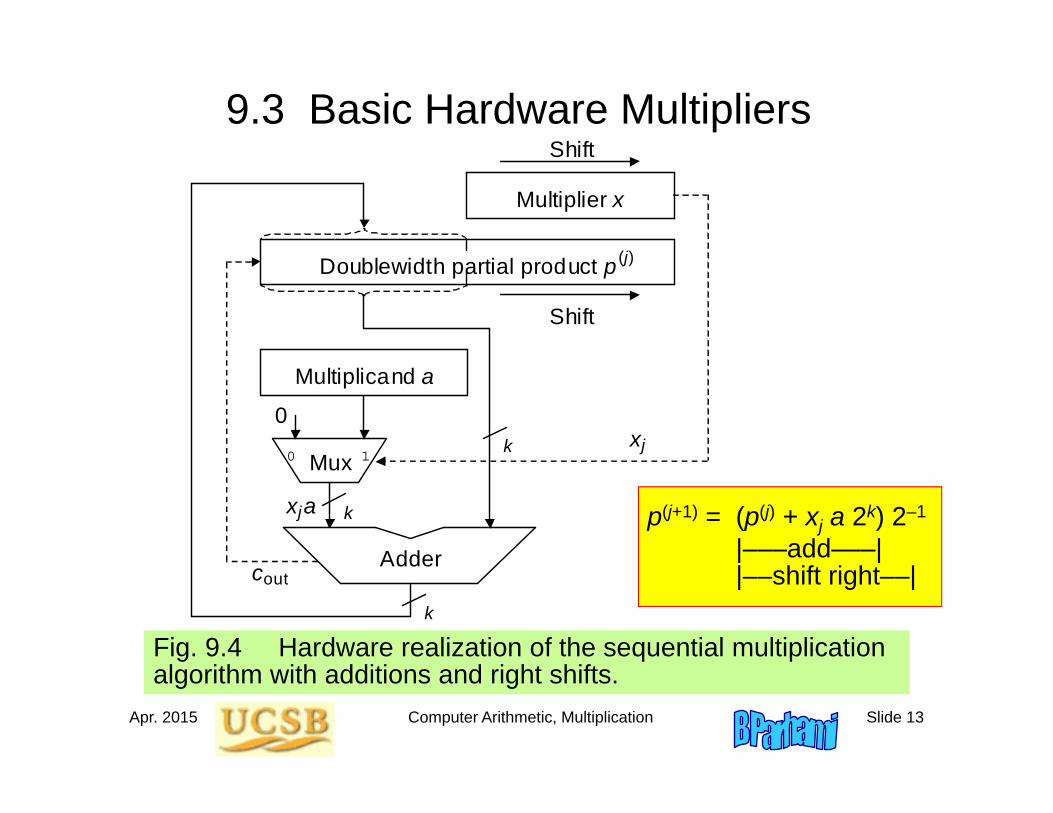
9.3 Basic Hardware Multipliers

Fig. 9.4 Hardware realization of the sequential multiplication algorithm with additions and right shifts.

Multiplier x

Mux

Adder

0

out c

0 1

Doublewidth partial product p

Multiplicand a

Shift

Shift

(j)

j x

x a j

k

k

k p(j+1) = (p(j) + xj a 2k) 2–1



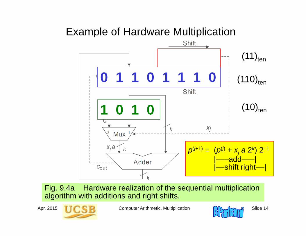
Example of Hardware Multiplication

Fig. 9.4a Hardware realization of the sequential multiplication algorithm with additions and right shifts.

1 0 1 1

1 0 1 0

0 0 0 01 0 1 01 0 1

0 1 0 1 01 1 1 1 01 0

0 1 1 1 1 01

0 0 1 1 1 1 01 1 0 1 1 1 00 1 1 0 1 1 1 0(11)ten

(10)ten

(110)ten

p(j+1) = (p(j) + xj a 2k) 2–1



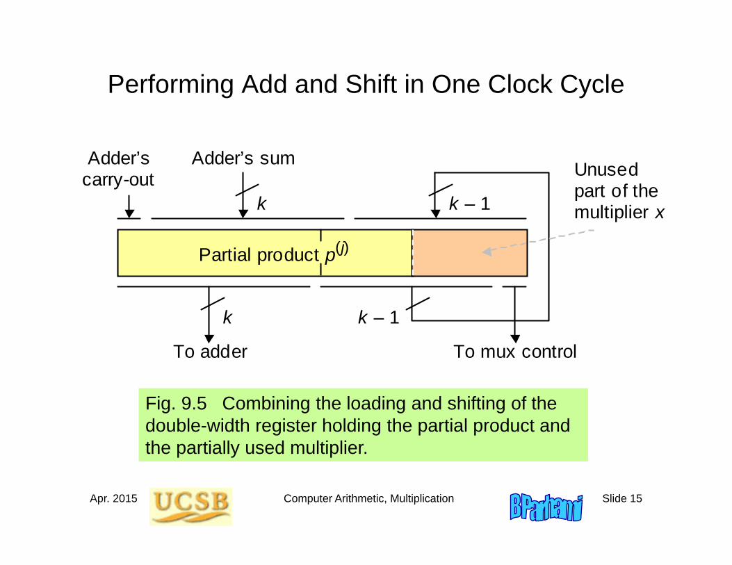
Performing Add and Shift in One Clock Cycle

Partial product p (j)

k

Unused part of the multiplier x

Adder’s carry-out

Adder’s sum

k

k – 1

k – 1

To mux control To adder

Fig. 9.5 Combining the loading and shifting of the double-width register holding the partial product and the partially used multiplier.


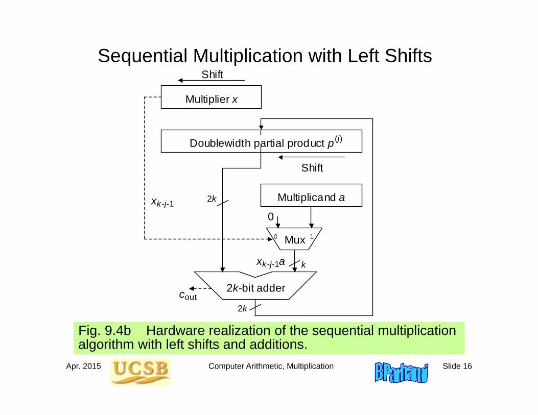
Sequential Multiplication with Left Shifts

Fig. 9.4b Hardware realization of the sequential multiplication algorithm with left shifts and additions.

Multiplier x

Mux

2k-bit adder

0

out c

0 1

Doublewidth partial product p

Multiplicand a

Shift

Shift

(j)

k-j-1 x

a

2k

k k-j-1 x

2k


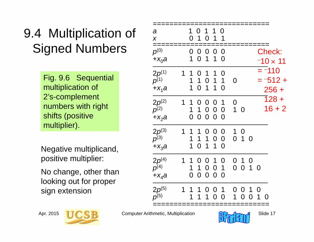
9.4 Multiplication of Signed Numbers

Fig. 9.6 Sequential multiplication of 2’s-complement numbers with right shifts (positive multiplier).

============================a 1 0 1 1 0x 0 1 0 1 1============================p(0) 0 0 0 0 0+x0a 1 0 1 1 0–––––––––––––––––––––––––––––2p(1) 1 1 0 1 1 0p(1) 1 1 0 1 1 0+x1a 1 0 1 1 0–––––––––––––––––––––––––––––2p(2) 1 1 0 0 0 1 0p(2) 1 1 0 0 0 1 0+x2a 0 0 0 0 0–––––––––––––––––––––––––––––2p(3) 1 1 1 0 0 0 1 0p(3) 1 1 1 0 0 0 1 0+x3a 1 0 1 1 0–––––––––––––––––––––––––––––2p(4) 1 1 0 0 1 0 0 1 0p(4) 1 1 0 0 1 0 0 1 0+x4a 0 0 0 0 0–––––––––––––––––––––––––––––2p(5) 1 1 1 0 0 1 0 0 1 0p(5) 1 1 1 0 0 1 0 0 1 0============================

Negative multiplicand,positive multiplier:

No change, other than looking out for propersign extension

Check:–10 11= –110= –512 +

256 + 128 + 16 + 2


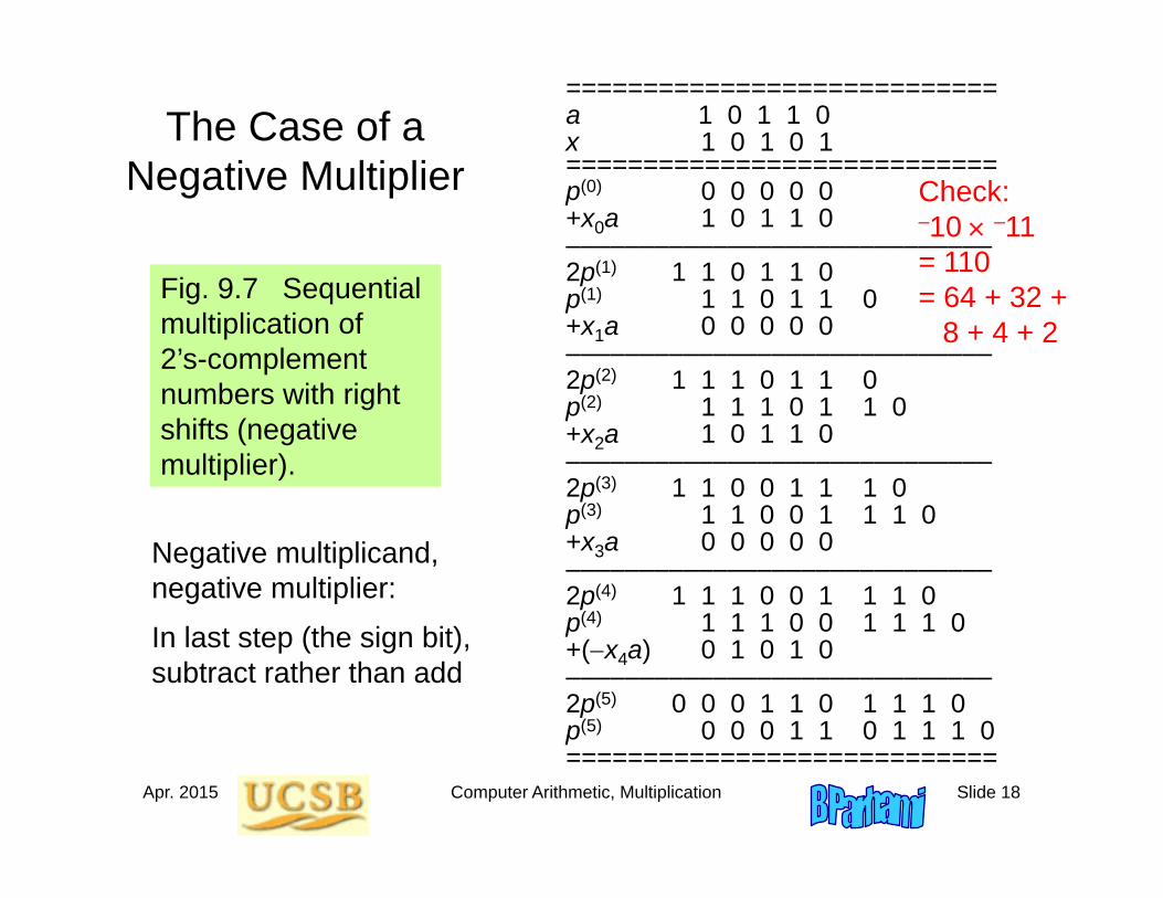
The Case of a Negative Multiplier

Fig. 9.7 Sequential multiplication of 2’s-complement numbers with right shifts (negative multiplier).

============================a 1 0 1 1 0x 1 0 1 0 1============================p(0) 0 0 0 0 0+x0a 1 0 1 1 0–––––––––––––––––––––––––––––2p(1) 1 1 0 1 1 0p(1) 1 1 0 1 1 0+x1a 0 0 0 0 0–––––––––––––––––––––––––––––2p(2) 1 1 1 0 1 1 0p(2) 1 1 1 0 1 1 0+x2a 1 0 1 1 0–––––––––––––––––––––––––––––2p(3) 1 1 0 0 1 1 1 0p(3) 1 1 0 0 1 1 1 0+x3a 0 0 0 0 0–––––––––––––––––––––––––––––2p(4) 1 1 1 0 0 1 1 1 0p(4) 1 1 1 0 0 1 1 1 0+(x4a) 0 1 0 1 0–––––––––––––––––––––––––––––2p(5) 0 0 0 1 1 0 1 1 1 0p(5) 0 0 0 1 1 0 1 1 1 0============================

Negative multiplicand,negative multiplier:

In last step (the sign bit), subtract rather than add

Check:–10 –11= 110= 64 + 32 +

8 + 4 + 2


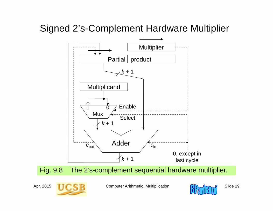
Signed 2’s-Complement Hardware Multiplier

Fig. 9.8 The 2’s-complement sequential hardware multiplier.

Adder

k + 1

0, except in last cycle

01Mux

k + 1

Enable

Select

Partial product

Multiplier

Multiplicand

k + 1

cincout


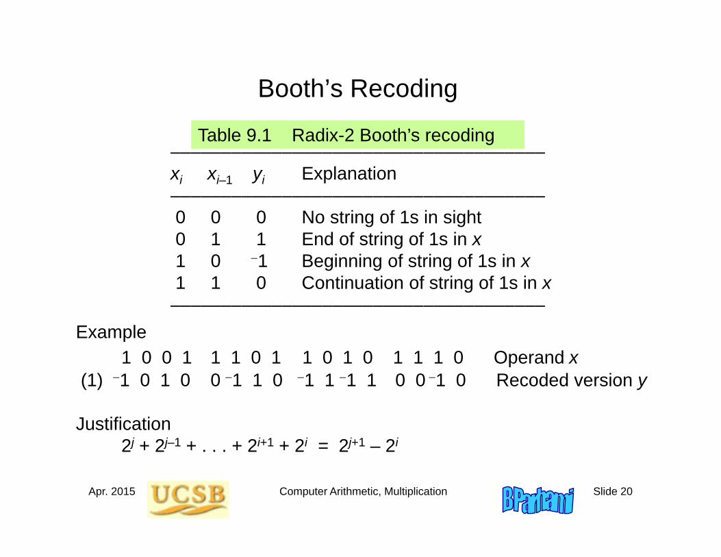
Booth’s Recoding

Table 9.1 Radix-2 Booth’s recoding–––––––––––––––––––––––––––––––––––––xi xi–1 yi Explanation–––––––––––––––––––––––––––––––––––––0 0 0 No string of 1s in sight0 1 1 End of string of 1s in x1 0 1 Beginning of string of 1s in x1 1 0 Continuation of string of 1s in x–––––––––––––––––––––––––––––––––––––

Example1 0 0 1 1 1 0 1 1 0 1 0 1 1 1 0 Operand x

(1) 1 0 1 0 0 1 1 0 1 1 1 1 0 0 1 0 Recoded version y

Justification2j + 2j–1 + . . . + 2i+1 + 2i = 2j+1 – 2i


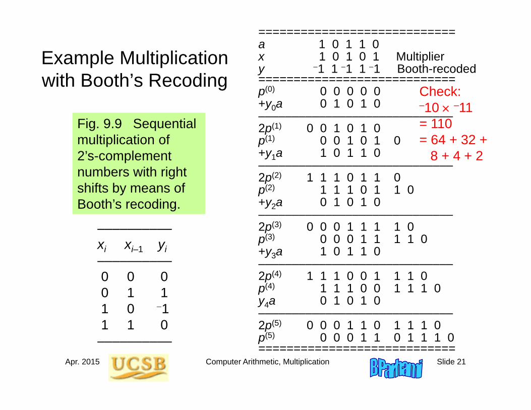
Example Multiplication with Booth’s Recoding

Fig. 9.9 Sequential multiplication of 2’s-complement numbers with right shifts by means of Booth’s recoding.

============================a 1 0 1 1 0x 1 0 1 0 1 Multipliery 1 1 1 1 1 Booth-recoded============================p(0) 0 0 0 0 0+y0a 0 1 0 1 0–––––––––––––––––––––––––––––2p(1) 0 0 1 0 1 0p(1) 0 0 1 0 1 0+y1a 1 0 1 1 0–––––––––––––––––––––––––––––2p(2) 1 1 1 0 1 1 0p(2) 1 1 1 0 1 1 0+y2a 0 1 0 1 0–––––––––––––––––––––––––––––2p(3) 0 0 0 1 1 1 1 0p(3) 0 0 0 1 1 1 1 0+y3a 1 0 1 1 0–––––––––––––––––––––––––––––2p(4) 1 1 1 0 0 1 1 1 0p(4) 1 1 1 0 0 1 1 1 0y4a 0 1 0 1 0–––––––––––––––––––––––––––––2p(5) 0 0 0 1 1 0 1 1 1 0p(5) 0 0 0 1 1 0 1 1 1 0============================

––––––––––xi xi–1 yi––––––––––0 0 00 1 11 0 11 1 0––––––––––

Check:–10 –11= 110= 64 + 32 +

8 + 4 + 2


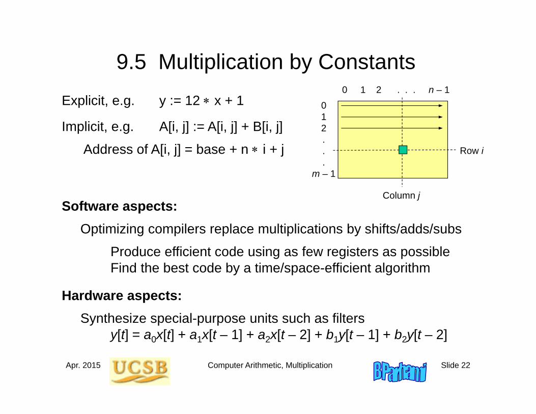
9.5 Multiplication by ConstantsExplicit, e.g. y := 12 x + 1

Implicit, e.g. A[i, j] := A[i, j] + B[i, j]

Address of A[i, j] = base + n i + j

Software aspects:Optimizing compilers replace multiplications by shifts/adds/subs

Produce efficient code using as few registers as possible Find the best code by a time/space-efficient algorithm

0 1 2 . . . n – 1 0 1 2 ...

m – 1

Row i

Column j

Hardware aspects:Synthesize special-purpose units such as filters

y[t] = a0x[t] + a1x[t – 1] + a2x[t – 2] + b1y[t – 1] + b2y[t – 2]


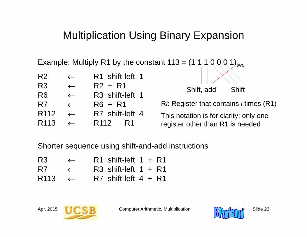
Multiplication Using Binary Expansion

Example: Multiply R1 by the constant 113 = (1 1 1 0 0 0 1)two

R2 R1 shift-left 1R3 R2 + R1R6 R3 shift-left 1R7 R6 + R1R112 R7 shift-left 4R113 R112 + R1

Shift, add Shift

Ri: Register that contains i times (R1)

This notation is for clarity; only one register other than R1 is needed

Shorter sequence using shift-and-add instructions

R3 R1 shift-left 1 + R1R7 R3 shift-left 1 + R1R113 R7 shift-left 4 + R1


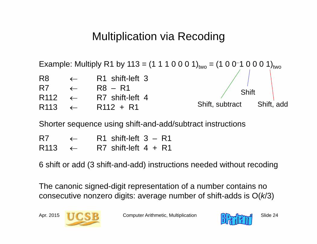
Multiplication via Recoding

Example: Multiply R1 by 113 = (1 1 1 0 0 0 1)two = (1 0 01 0 0 0 1)two

R8 R1 shift-left 3R7 R8 – R1R112 R7 shift-left 4R113 R112 + R1 Shift, add

Shift

Shorter sequence using shift-and-add/subtract instructions

R7 R1 shift-left 3 – R1R113 R7 shift-left 4 + R1

Shift, subtract

6 shift or add (3 shift-and-add) instructions needed without recoding

The canonic signed-digit representation of a number contains no consecutive nonzero digits: average number of shift-adds is O(k/3)


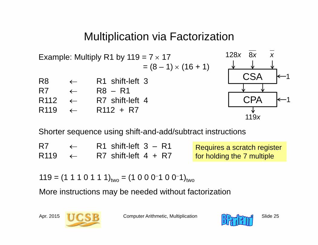
Multiplication via Factorization

Example: Multiply R1 by 119 = 7 17 = (8 – 1) (16 + 1)

R8 R1 shift-left 3R7 R8 – R1R112 R7 shift-left 4R119 R112 + R7

Shorter sequence using shift-and-add/subtract instructions

R7 R1 shift-left 3 – R1R119 R7 shift-left 4 + R7

119 = (1 1 1 0 1 1 1)two = (1 0 0 01 0 01)two

More instructions may be needed without factorization

Requires a scratch register for holding the 7 multiple

CSA

CPA

128x 8x x

119x

1

1


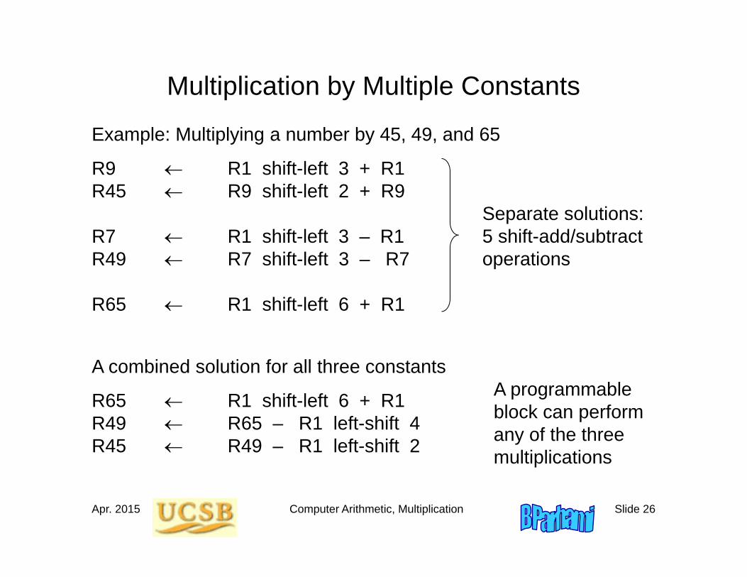
Multiplication by Multiple Constants

Example: Multiplying a number by 45, 49, and 65

R9 R1 shift-left 3 + R1R45 R9 shift-left 2 + R9

R7 R1 shift-left 3 – R1R49 R7 shift-left 3 – R7

R65 R1 shift-left 6 + R1

A combined solution for all three constants

R65 R1 shift-left 6 + R1R49 R65 – R1 left-shift 4R45 R49 – R1 left-shift 2

Separate solutions:5 shift-add/subtractoperations

A programmable block can perform any of the three multiplications


9.6 Preview of Fast MultipliersViewing multiplication as a multioperand addition problem,there are but two ways to speed it up

a. Reducing the number of operands to be added:Handling more than one multiplier bit at a time(high-radix multipliers, Chapter 10)

b. Adding the operands faster:Parallel/pipelined multioperand addition(tree and array multipliers, Chapter 11)

In Chapter 12, we cover all remaining multiplication topics:

Bit-serial multipliersModular multipliersMultiply-add unitsSquaring as a special case


10 High-Radix Multipliers

Chapter GoalsStudy techniques that allow us to handlemore than one multiplier bit in each cycle(two bits in radix 4, three in radix 8, . . .)

Chapter HighlightsHigh radix gives rise to “difficult” multiplesRecoding (change of digit-set) as remedyCarry-save addition reduces cycle timeImplementation and optimization methods


High-Radix Multipliers: Topics


10.1 Radix-4 Multiplication

10.2 Modified Booth’s Recoding

10.3 Using Carry-Save Adders

10.4 Radix-8 and Radix-16 Multipliers

10.5 Multibeat Multipliers

10.6 VLSI Complexity Issues


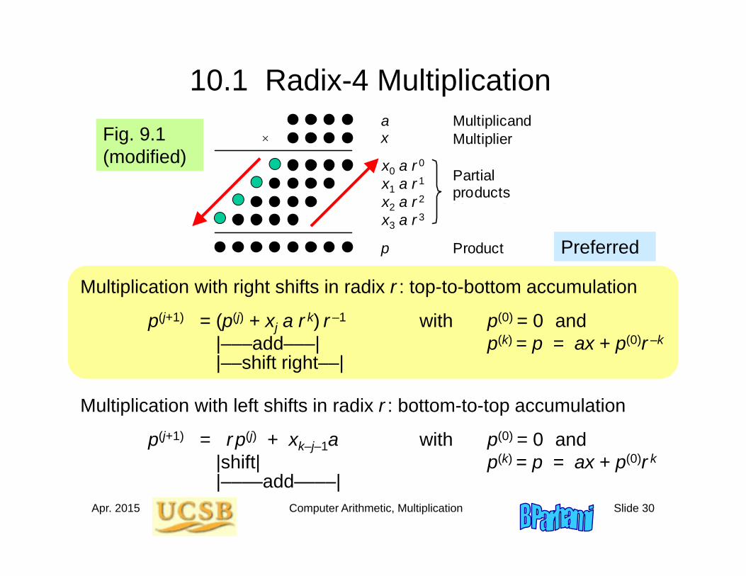
10.1 Radix-4 Multiplication

Preferred

Multiplication with right shifts in radix r : top-to-bottom accumulation

p(j+1) = (p(j) + xj a r k) r –1 with p(0) = 0 and|–––add–––| p(k) = p = ax + p(0)r –k

|––shift right––|

Multiplication with left shifts in radix r : bottom-to-top accumulation

p(j+1) = rp(j) + xk–j–1a with p(0) = 0 and|shift| p(k) = p = ax + p(0)r k

|––––add––––|

Fig. 9.1 (modified)

Product


a x

p

2

x a

0 0

1 x a 2 1 x a 2

2 2

2 3 3

x a


x0 a r 0

x1 a r 1

x2 a r 2

x3 a r 3


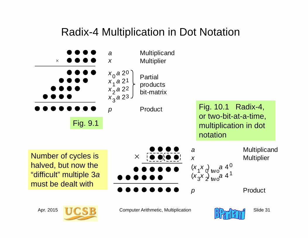
Radix-4 Multiplication in Dot Notation

Number of cycles is halved, but now the “difficult” multiple 3amust be dealt with

Product


a x

p

2

x a

0 0

1 x a 2 1 x a 2

2 2

2 3 3

x a


Multiplier x

p Product

Multiplicand a

(x x ) a 4 1 3 2 two

4 0 a (x x ) 1 0 two

Fig. 9.1

Fig. 10.1 Radix-4, or two-bit-at-a-time, multiplication in dot notation


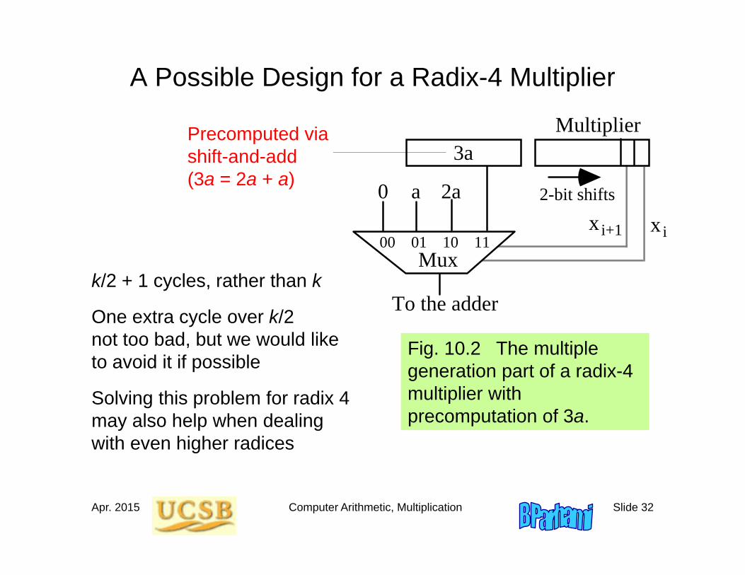
A Possible Design for a Radix-4 Multiplier

Precomputed via shift-and-add(3a = 2a + a)

k/2 + 1 cycles, rather than k

One extra cycle over k/2 not too bad, but we would like to avoid it if possible

Solving this problem for radix 4 may also help when dealing with even higher radices

0 a 2a

3aMultiplier

To the adder

2-bit shifts

00 01 10 11Mux

xi+1 xi

Fig. 10.2 The multiple generation part of a radix-4 multiplier with precomputation of 3a.


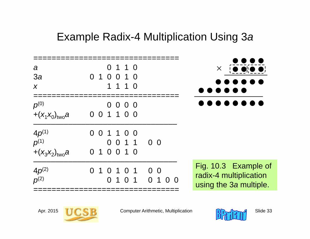
Example Radix-4 Multiplication Using 3a

================================a 0 1 1 03a 0 1 0 0 1 0x 1 1 1 0================================p(0) 0 0 0 0+(x1x0)twoa 0 0 1 1 0 0–––––––––––––––––––––––––––––––––4p(1) 0 0 1 1 0 0p(1) 0 0 1 1 0 0+(x3x2)twoa 0 1 0 0 1 0–––––––––––––––––––––––––––––––––4p(2) 0 1 0 1 0 1 0 0p(2) 0 1 0 1 0 1 0 0================================

Fig. 10.3 Example of radix-4 multiplication using the 3a multiple.

x

p

a

(x x )3 2

(x x )1 0


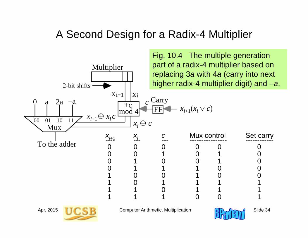
A Second Design for a Radix-4 Multiplier

xi+1 xi c Mux control Set carry---- --- --- ---------------- ------------0 0 0 0 0 00 0 1 0 1 00 1 0 0 1 00 1 1 1 0 01 0 0 1 0 01 0 1 1 1 11 1 0 1 1 11 1 1 0 0 1

Fig. 10.4 The multiple generation part of a radix-4 multiplier based on replacing 3a with 4a (carry into next higher radix-4 multiplier digit) and –a.

0 a 2a –a

Multiplier

To the adder

+c FF Set if = = 1 or if = c = 1c

00 01 10 11Mux

2-bit shifts

mod 4Carry

xi+1 xi

xi+1xi+1

xixi+1(xi c)xi+1 xi c xi c

c


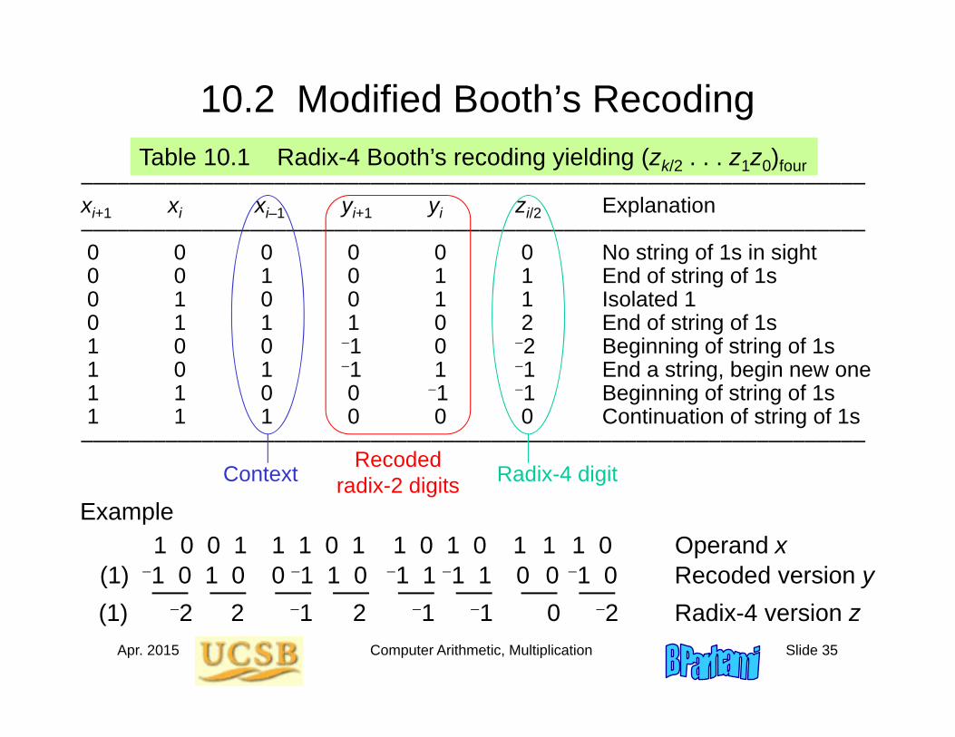
10.2 Modified Booth’s RecodingTable 10.1 Radix-4 Booth’s recoding yielding (zk/2 . . . z1z0)four

–––––––––––––––––––––––––––––––––––––––––––––––––––––––––––––––––xi+1 xi xi–1 yi+1 yi zi/2 Explanation–––––––––––––––––––––––––––––––––––––––––––––––––––––––––––––––––0 0 0 0 0 0 No string of 1s in sight0 0 1 0 1 1 End of string of 1s0 1 0 0 1 1 Isolated 10 1 1 1 0 2 End of string of 1s1 0 0 1 0 2 Beginning of string of 1s1 0 1 1 1 1 End a string, begin new one1 1 0 0 1 1 Beginning of string of 1s1 1 1 0 0 0 Continuation of string of 1s–––––––––––––––––––––––––––––––––––––––––––––––––––––––––––––––––

(1) 2 2 1 2 1 1 0 2 Radix-4 version z

ContextRecoded

radix-2 digits Radix-4 digit

Example1 0 0 1 1 1 0 1 1 0 1 0 1 1 1 0 Operand x

(1) 1 0 1 0 0 1 1 0 1 1 1 1 0 0 1 0 Recoded version y


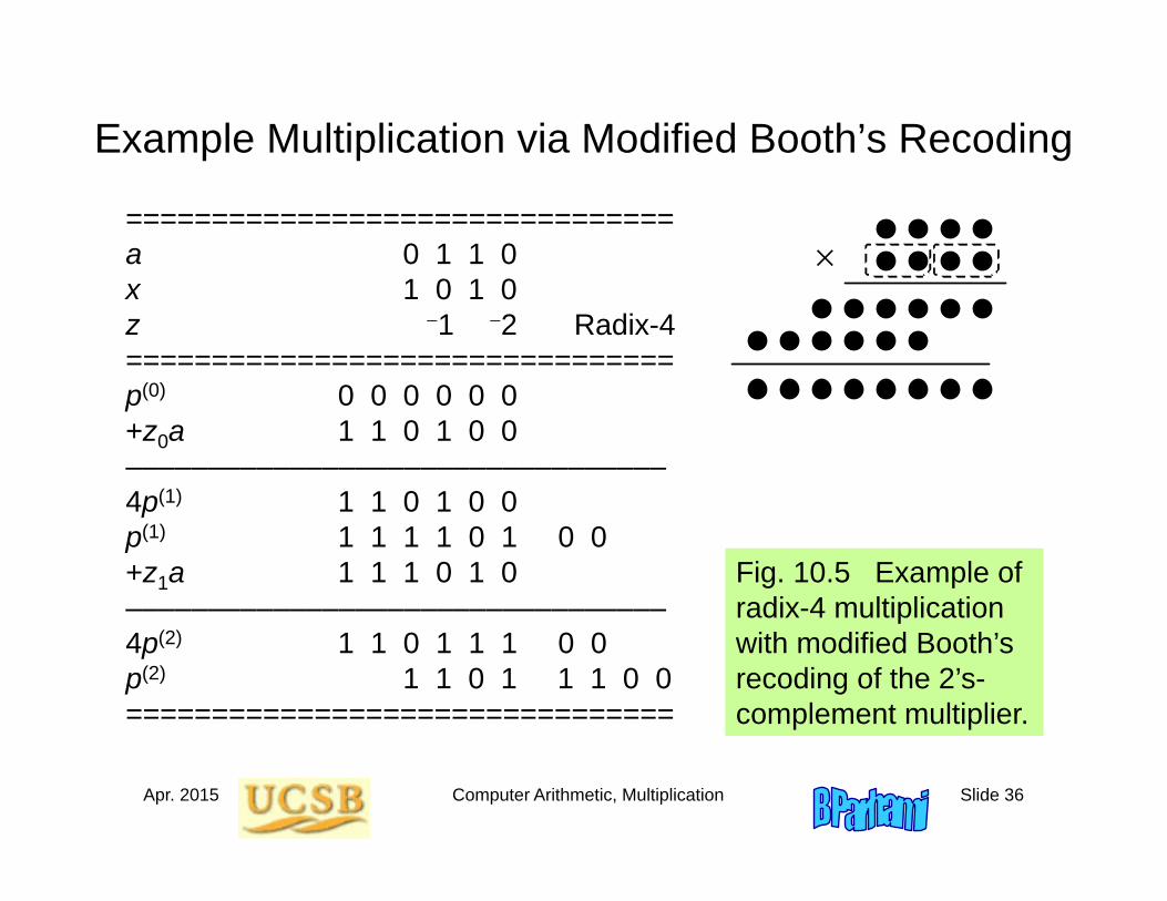
Example Multiplication via Modified Booth’s Recoding

================================a 0 1 1 0x 1 0 1 0z 1 2 Radix-4================================p(0) 0 0 0 0 0 0+z0a 1 1 0 1 0 0–––––––––––––––––––––––––––––––––4p(1) 1 1 0 1 0 0p(1) 1 1 1 1 0 1 0 0+z1a 1 1 1 0 1 0–––––––––––––––––––––––––––––––––4p(2) 1 1 0 1 1 1 0 0p(2) 1 1 0 1 1 1 0 0================================

Fig. 10.5 Example of radix-4 multiplication with modified Booth’s recoding of the 2’s-complement multiplier.

x

p

a

(x x )3 2

(x x )1 0


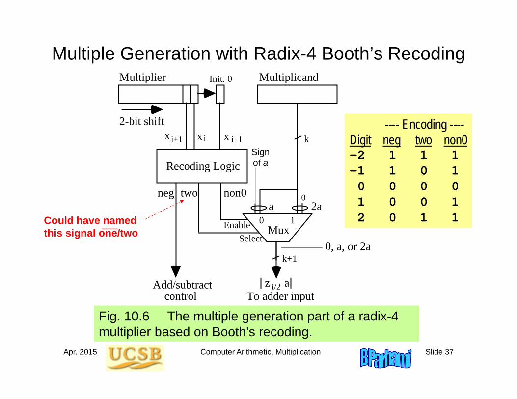
Multiple Generation with Radix-4 Booth’s Recoding

Fig. 10.6 The multiple generation part of a radix-4 multiplier based on Booth’s recoding.

Could have named this signal one/two

two non0a 2a

EnableSelect

z a

neg

ii+1 i–1

i/2

0 1Mux

k+10, a, or 2a

To adder inputAdd/subtract control

x

Multiplier

xx

Recoding Logic

Multiplicand

0

k

0

2-bit shift

Init. 0

Sign of a

---- Encoding ----Digit neg two non0–2 1 1 1 –1 1 0 1 0 0 0 01 0 0 12 0 1 1


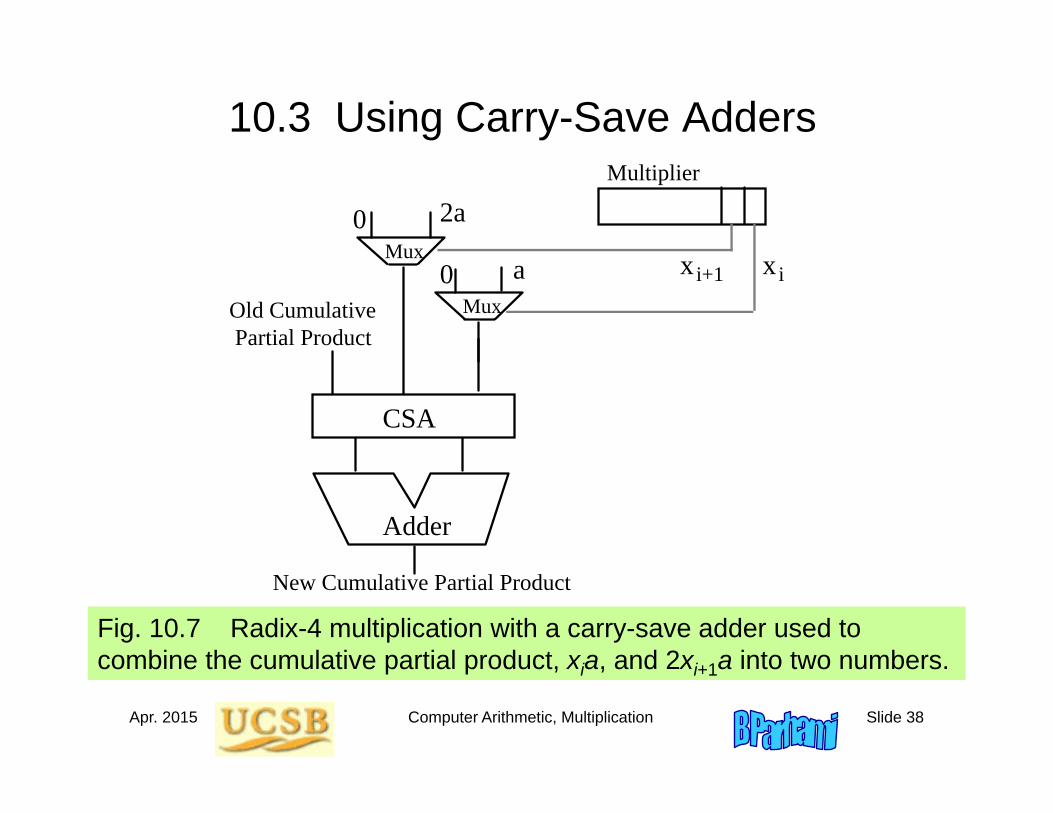
10.3 Using Carry-Save Adders

Fig. 10.7 Radix-4 multiplication with a carry-save adder used to combine the cumulative partial product, xia, and 2xi+1a into two numbers.

Mux

0 2a

0 a

Multiplier

New Cumulative Partial Product

Old Cumulative Partial Product

CSA

Mux xi+1 xi

Adder


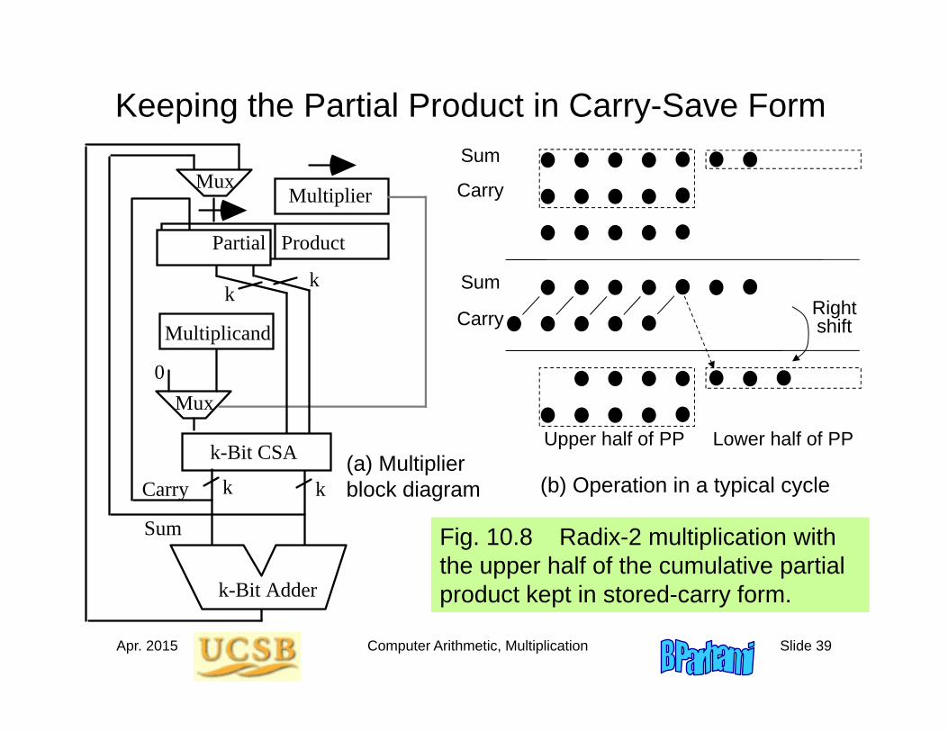
Keeping the Partial Product in Carry-Save Form

Fig. 10.8 Radix-2 multiplication with the upper half of the cumulative partial product kept in stored-carry form.

0

Multiplier

k

k

k-Bit CSA

k

Partial Product

k

Mux

k-Bit Adder

Mux

Multiplicand

Carry

Sum

Upper half of PP Lower half of PP

Right shift

Sum

Carry

Sum

Carry

(a) Multiplier block diagram (b) Operation in a typical cycle


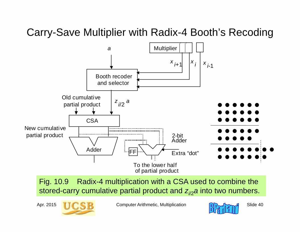
Carry-Save Multiplier with Radix-4 Booth’s Recoding

Fig. 10.9 Radix-4 multiplication with a CSA used to combine the stored-carry cumulative partial product and zi/2a into two numbers.

a

Multiplier

x i+1

x i

Adder

New cumulative partial product

Old cumulative partial product

FF

2-bit Adder

To the lower half of partial product

Booth recoder and selector

CSA

x i-1

z a i/2

Extra “dot”


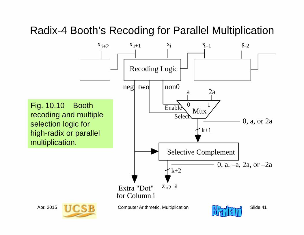
Radix-4 Booth’s Recoding for Parallel Multiplication

Fig. 10.10 Booth recoding and multiple selection logic for high-radix or parallel multiplication.

x x x x

Recoding Logic

two non0a 2a

EnableSelect

z a

neg

ii+1 i–1

i/2

i–2

0 1Mux

k+10, a, or 2a

k+2

Selective Complement

0, a, –a, 2a, or –2a

Extra "Dot" for Column i

xi+2


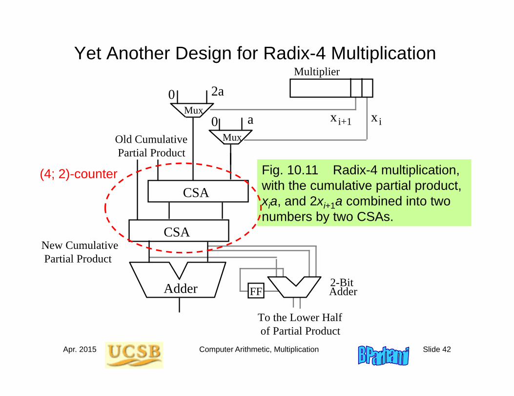
Yet Another Design for Radix-4 Multiplication

Fig. 10.11 Radix-4 multiplication, with the cumulative partial product, xia, and 2xi+1a combined into two numbers by two CSAs.

Mux

0 2a

0 a

Multiplier

CSA

Mux xi+1 xi

Adder

CSANew Cumulative Partial Product

Old Cumulative Partial Product

FF2-BitAdder

To the Lower Half of Partial Product

(4; 2)-counter


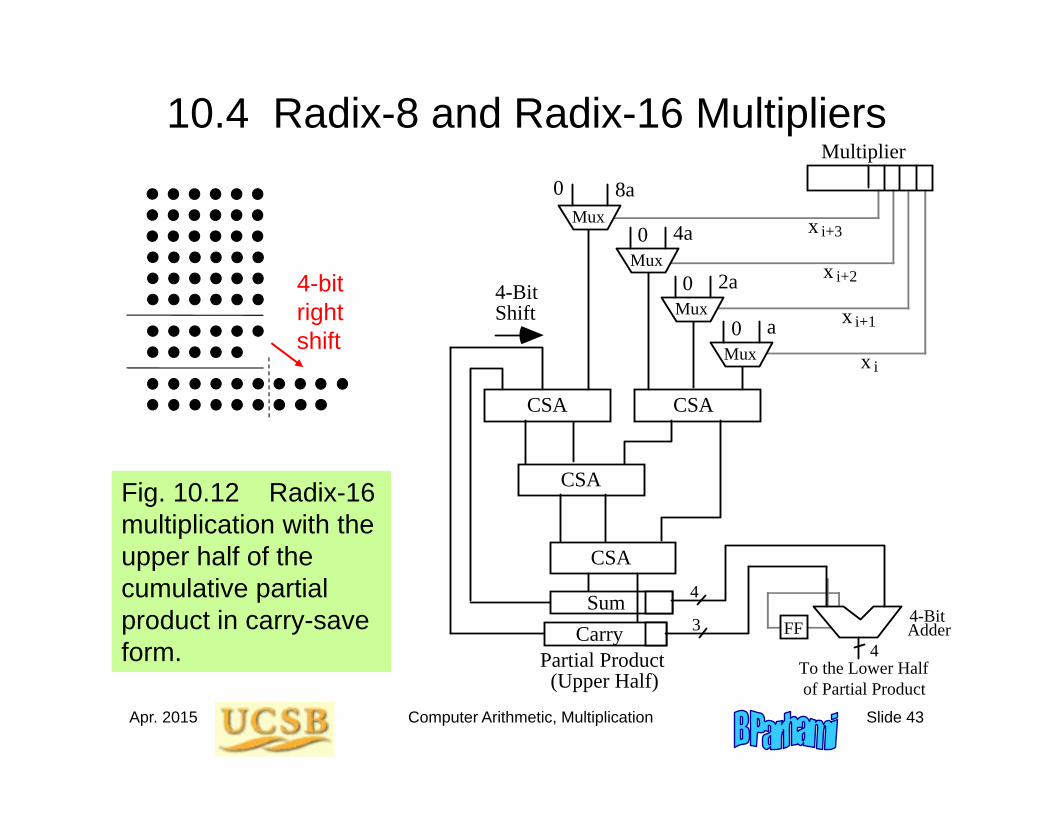
10.4 Radix-8 and Radix-16 Multipliers

Fig. 10.12 Radix-16 multiplication with the upper half of the cumulative partial product in carry-save form.

Multiplier

CSA CSA

CSA

CSA

Partial Product (Upper Half)

Mux0 8a

Mux0 4a

Mux0 2a

Mux0 a

x i+3

x i+2

x i+1

x i

CarrySum

4-Bit Shift

FF


3 4-BitAdder

4

4

4-bitrightshift


Other High-Radix MultipliersMultiplier

CSA CSA

CSA

CSA

Partial Product (Upper Half)

Mux0 8a

Mux0 4a

Mux0 2a

Mux0 a

xi+3

xi+2

xi+1

xi

CarrySum

4-Bit Shift

FF


3 4-BitAdder

4

4

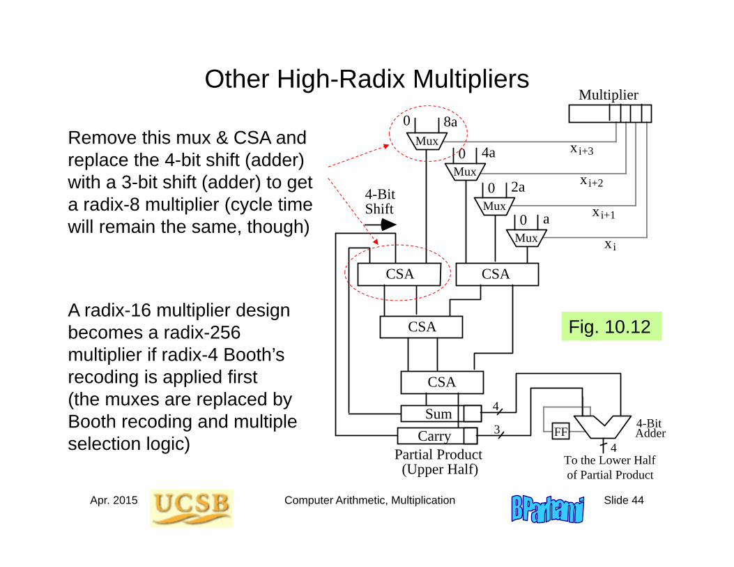
Fig. 10.12A radix-16 multiplier design becomes a radix-256 multiplier if radix-4 Booth’s recoding is applied first (the muxes are replaced by Booth recoding and multiple selection logic)

Remove this mux & CSA and replace the 4-bit shift (adder) with a 3-bit shift (adder) to get a radix-8 multiplier (cycle time will remain the same, though)


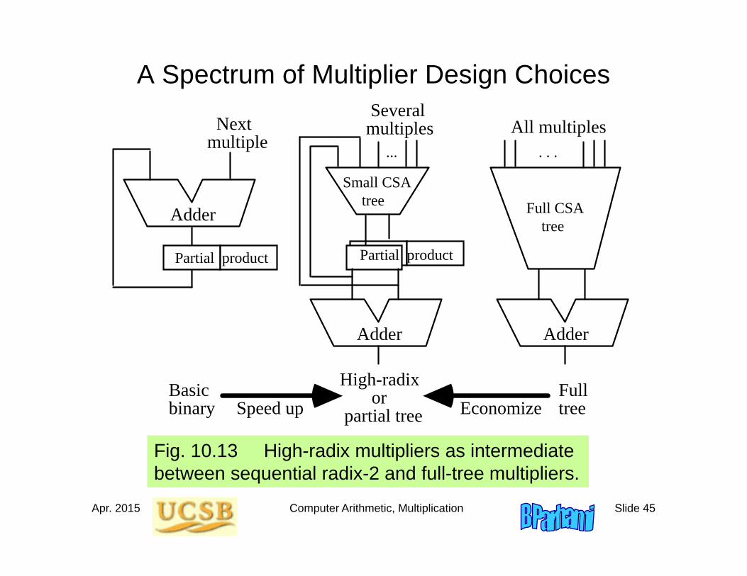
A Spectrum of Multiplier Design Choices

Basic binary

Adder

Adder

Next multiple

Partial product

...

Several multiples

Adder

. . .All multiples

Small CSA tree Full CSA

tree

High-radix or partial tree

Full treeSpeed up Economize

Partial product

Fig. 10.13 High-radix multipliers as intermediate between sequential radix-2 and full-tree multipliers.


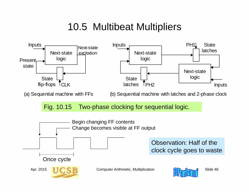
10.5 Multibeat Multipliers

Observation: Half of the clock cycle goes to waste

Fig. 10.15 Two-phase clocking for sequential logic.

Next-state logic

State flip-flops

Inputs Next-state excitation

Present state

Next-state logic

State latches

Inputs

Next-state logic

InputsState

latches

PH1

PH2 CLK

(a) Sequential machine with FFs (b) Sequential machine with latches and 2-phase clock

Once cycle

Begin changing FF contentsChange becomes visible at FF output


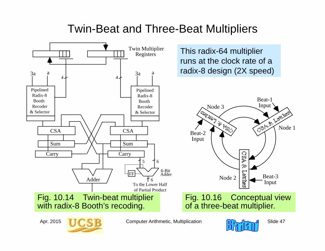
Twin-Beat and Three-Beat Multipliers

This radix-64 multiplier runs at the clock rate of a radix-8 design (2X speed)

Fig. 10.14 Twin-beat multiplier with radix-8 Booth’s recoding.

Adder

CSA

Sum

Carry

CSA

Sum

Carry

FF


6-BitAdder

6

65

Pipelined Radix-8 Booth Recoder & Selector

3a a 3a a4 4

Twin Multiplier Registers

Pipelined Radix-8 Booth Recoder & Selector

Beat-1 Input

Beat-3 Input

Beat-2 Input

Node 1

Node 2

Node 3

Fig. 10.16 Conceptual view of a three-beat multiplier.


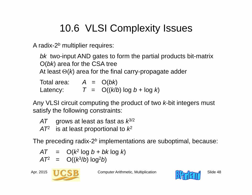
10.6 VLSI Complexity IssuesA radix-2b multiplier requires:

bk two-input AND gates to form the partial products bit-matrixO(bk) area for the CSA treeAt least (k) area for the final carry-propagate adder

Total area: A = O(bk)Latency: T = O((k/b) log b + log k)

Any VLSI circuit computing the product of two k-bit integers must satisfy the following constraints:

AT grows at least as fast as k3/2

AT2 is at least proportional to k2

The preceding radix-2b implementations are suboptimal, because:

AT = O(k2 log b + bk log k)AT2 = O((k3/b) log2b)


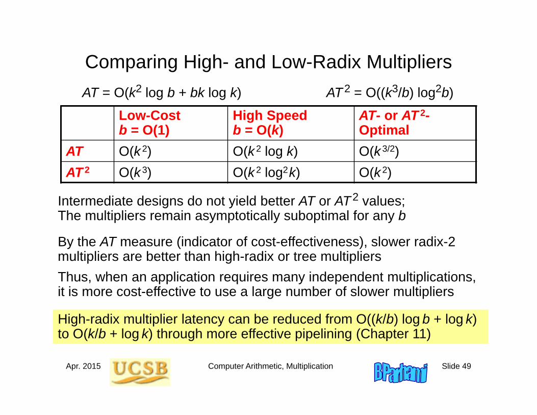
Comparing High- and Low-Radix Multipliers

Intermediate designs do not yield better AT or AT2 values;The multipliers remain asymptotically suboptimal for any b

Low-Costb = O(1)

High Speedb = O(k)

AT- or AT 2-Optimal

AT O(k2) O(k2 log k) O(k3/2)AT 2 O(k3) O(k2 log2k) O(k2)

AT = O(k2 log b + bk log k) AT2 = O((k3/b) log2b)

By the AT measure (indicator of cost-effectiveness), slower radix-2 multipliers are better than high-radix or tree multipliersThus, when an application requires many independent multiplications, it is more cost-effective to use a large number of slower multipliers

High-radix multiplier latency can be reduced from O((k/b) log b + log k) to O(k/b + log k) through more effective pipelining (Chapter 11)


11 Tree and Array Multipliers

Chapter GoalsStudy the design of multipliers for highestpossible performance (speed, throughput)

Chapter HighlightsTree multiplier = reduction tree

+ redundant-to-binary converterAvoiding full sign extension in multiplying

signed numbersArray multiplier = one-sided reduction tree

+ ripple-carry adder


Tree and Array Multipliers: Topics


11.1. Full-Tree Multipliers

11.2. Alternative Reduction Trees

11.3. Tree Multipliers for Signed Numbers

11.4. Partial-Tree and Truncated Multipliers

11.5. Array Multipliers

11.6. Pipelined Tree and Array Multipliers


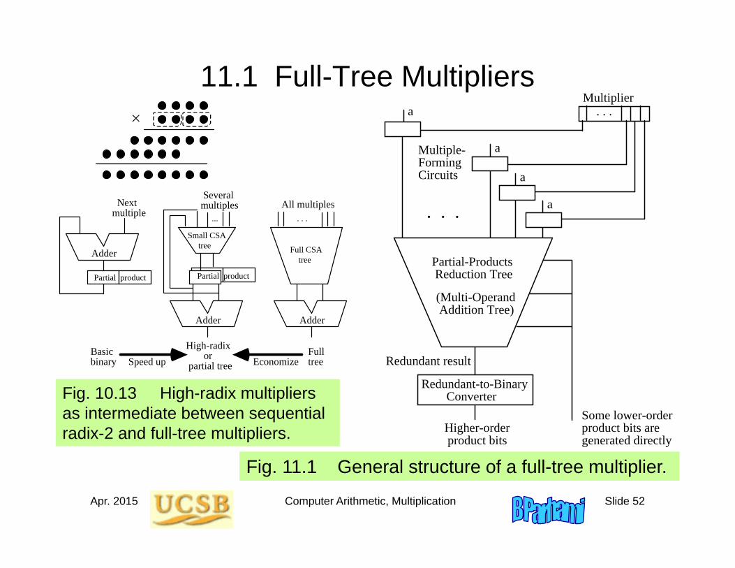
11.1 Full-Tree Multipliers

Basic binary

Adder

Adder

Next multiple

Partial product

...

Several multiples

Adder

. . .All multiples

Small CSA tree Full CSA

tree

High-radix or partial tree

Full treeSpeed up Economize

Partial product

Fig. 10.13 High-radix multipliers as intermediate between sequential radix-2 and full-tree multipliers. Higher-order

product bits

Multipliera

a

a

a. . .

. . .

Some lower-order product bits are generated directly

Redundant result

Redundant-to-Binary Converter

Multiple- Forming Circuits

(Multi-Operand Addition Tree)

Partial-Products Reduction Tree

Fig. 11.1 General structure of a full-tree multiplier.

Multiplier x

p Product

Multiplicand a

(x x ) a 4 1 3 2 two

4 0 a (x x ) 1 0 two


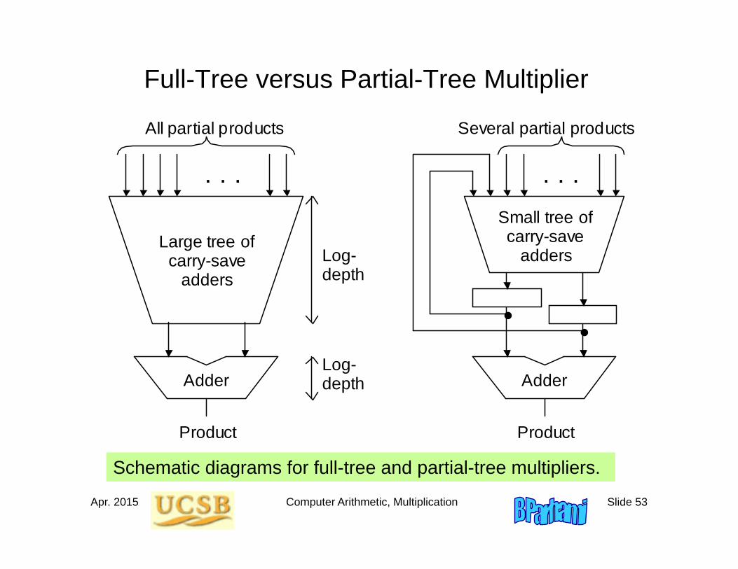
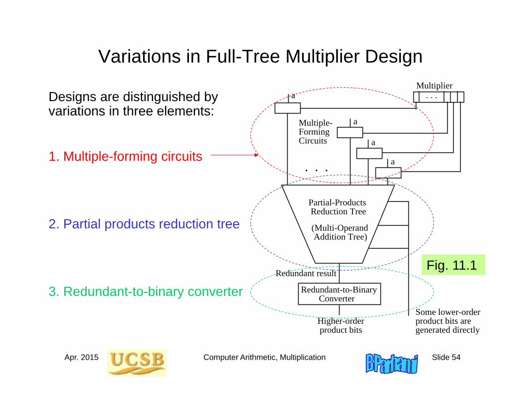
Full-Tree versus Partial-Tree Multiplier

Schematic diagrams for full-tree and partial-tree multipliers.

Adder

Large tree of carry-save

adders

. . .

All partial products

Product

Adder

Small tree of carry-save

adders

. . .

Several partial products

Product

Log-depth

Log-depth


Variations in Full-Tree Multiplier Design

Designs are distinguished by variations in three elements:

Higher-order product bits

Multipliera

a

a

a. . .

. . .

Some lower-order product bits are generated directly

Redundant result

Redundant-to-Binary Converter

Multiple- Forming Circuits

(Multi-Operand Addition Tree)

Partial-Products Reduction Tree

Fig. 11.1

2. Partial products reduction tree

3. Redundant-to-binary converter

1. Multiple-forming circuits


Product


a x

p

2

x a

0 0

1 x a 2 1 x a 2

2 2

2 3 3

x a


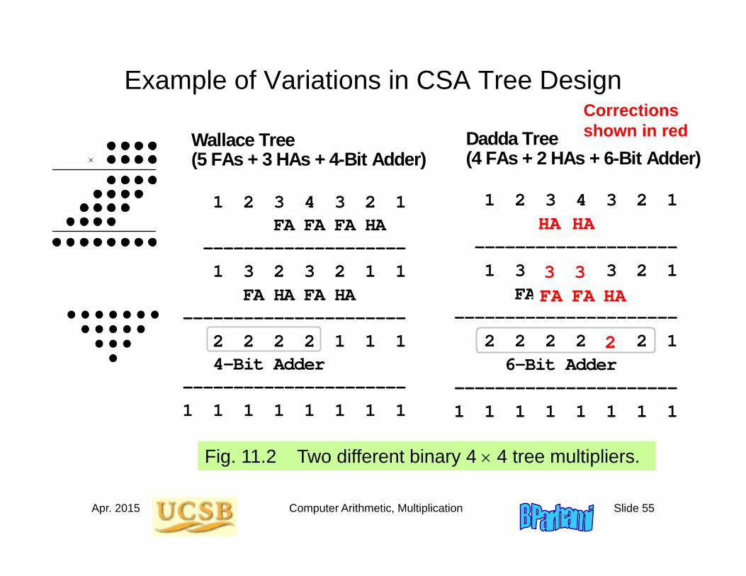
Example of Variations in CSA Tree Design

1 2 3 4 3 2 1 FA FA FA HA -------------------- 1 3 2 3 2 1 1 FA HA FA HA ---------------------- 2 2 2 2 1 1 1 4-Bit Adder ----------------------1 1 1 1 1 1 1 1

Wallace Tree (5 FAs + 3 HAs + 4-Bit Adder)

1 2 3 4 3 2 1 FA FA -------------------- 1 3 2 2 3 2 1 FA HA HA FA ---------------------- 2 2 2 2 1 2 1 6-Bit Adder ----------------------1 1 1 1 1 1 1 1

Dadda Tree (4 FAs + 2 HAs + 6-Bit Adder)

Fig. 11.2 Two different binary 4 4 tree multipliers.

HA

3

HA

3FAFA HA

Correctionsshown in red

2


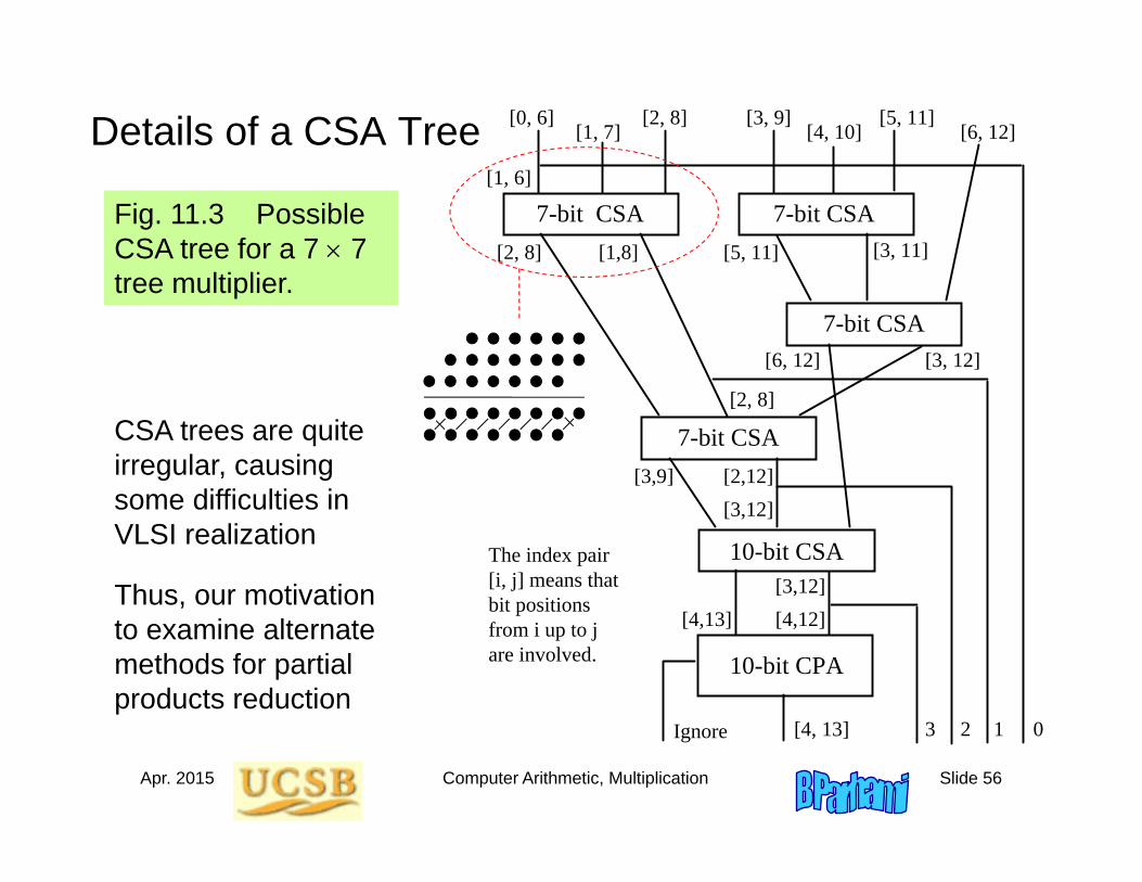
Details of a CSA Tree

Fig. 11.3 Possible CSA tree for a 7 7 tree multiplier.

CSA trees are quite irregular, causing some difficulties in VLSI realization

10-bit CPA

7-bit CSA 7-bit CSA

7-bit CSA

10-bit CSA

2Ignore

The index pair [i, j] means that bit positions from i up to j are involved.

7-bit CSA

[0, 6] [1, 7]

[2, 8] [6, 12]

[3, 11] [1,8]

[3, 9] [4, 10]

[5, 11]

[2, 8] [5, 11]

[6, 12]

[2,12]

[3, 12]

[4,13] [4,12]

[4, 13]

[3,9]

3

[3,12]

[2, 8]

[3,12]

[1, 6]

01

Thus, our motivation to examine alternate methods for partial products reduction


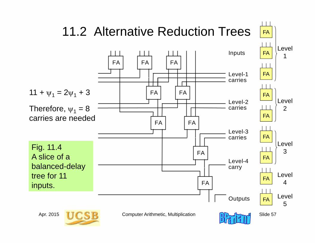
11.2 Alternative Reduction Trees

Fig. 11.4 A slice of a balanced-delay tree for 11 inputs.

FA FA FA

FA FA

FA FA

FA

FA

Inputs

Level-1 carries

Level-2 carries

Level-3 carries

Level-4 carry

Outputs

FA

FA

FA

FA

FA

FA

FA

FA

FA

11 + 1 = 21 + 3

Therefore, 1 = 8 carries are needed

Level1

Level5

Level4

Level3

Level2


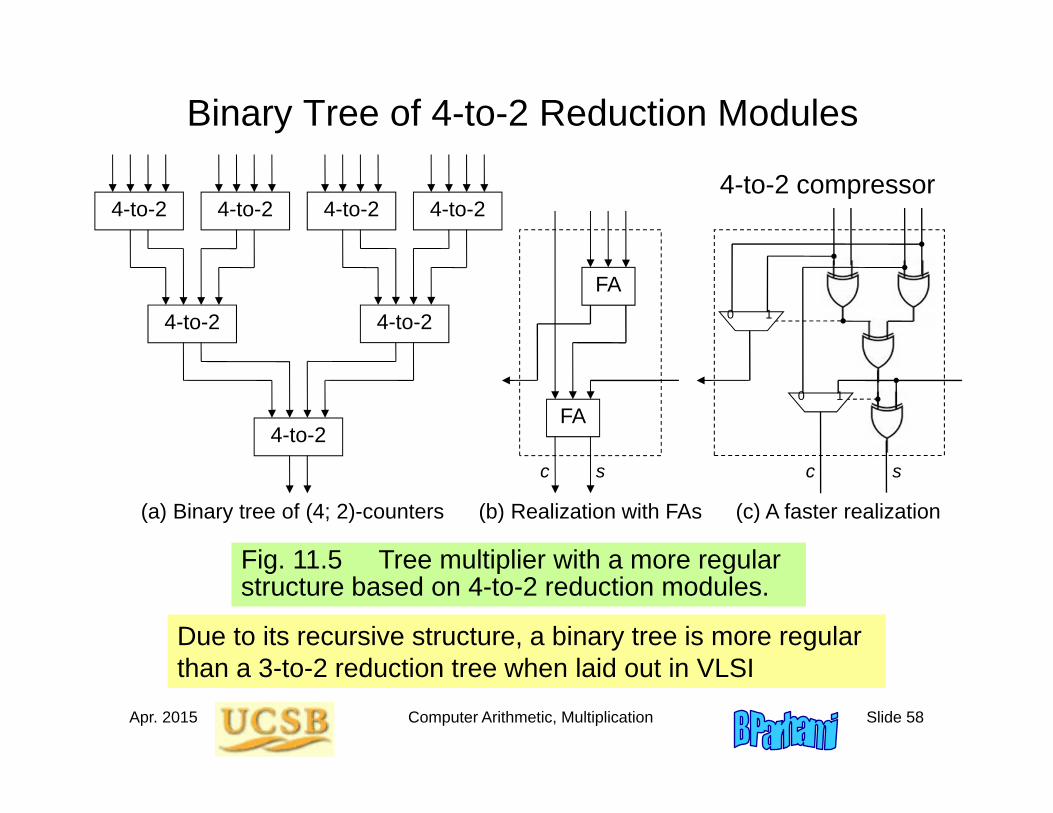
Binary Tree of 4-to-2 Reduction Modules

Due to its recursive structure, a binary tree is more regular than a 3-to-2 reduction tree when laid out in VLSI

Fig. 11.5 Tree multiplier with a more regular structure based on 4-to-2 reduction modules.

(a) Binary tree of (4; 2)-counters

4-to-2 4-to-2 4-to-2 4-to-2

4-to-2 4-to-2

4-to-2

(b) Realization with FAs (c) A faster realization

FA

FA

c s c s

0 1

0 1

4-to-2 compressor


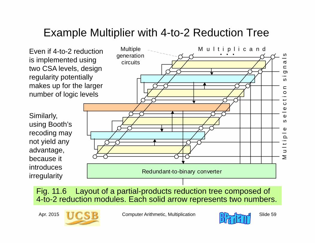
Example Multiplier with 4-to-2 Reduction Tree

Fig. 11.6 Layout of a partial-products reduction tree composed of 4-to-2 reduction modules. Each solid arrow represents two numbers.

M u l t i p l i c a n d . . .

Redundant-to-binary converter

Multiple generation

circuits

M u

l t i

p l

e s

e l

e c

t i o

n

s i g

n a

l s Even if 4-to-2 reduction

is implemented using two CSA levels, design regularity potentially makes up for the larger number of logic levels

Similarly, using Booth’s recoding may not yield any advantage, because it introduces irregularity


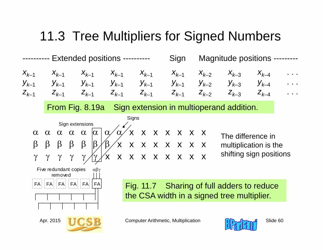
11.3 Tree Multipliers for Signed Numbers

From Fig. 8.19a Sign extension in multioperand addition.

---------- Extended positions ---------- Sign Magnitude positions ---------

xk–1 xk–1 xk–1 xk–1 xk–1 xk–1 xk–2 xk–3 xk–4 . . .yk–1 yk–1 yk–1 yk–1 yk–1 yk–1 yk–2 yk–3 yk–4 . . .zk–1 zk–1 zk–1 zk–1 zk–1 zk–1 zk–2 zk–3 zk–4 . . .

x

x

x

x

x

x

x

x

x

x

x

x

x

x

x

x

x

x

x

x

x

x

x x

FA FA FA FA FA FA

Five redundant copies removed

Sign extensions Signs

The difference in multiplication is the shifting sign positions

Fig. 11.7 Sharing of full adders to reduce the CSA width in a signed tree multiplier.


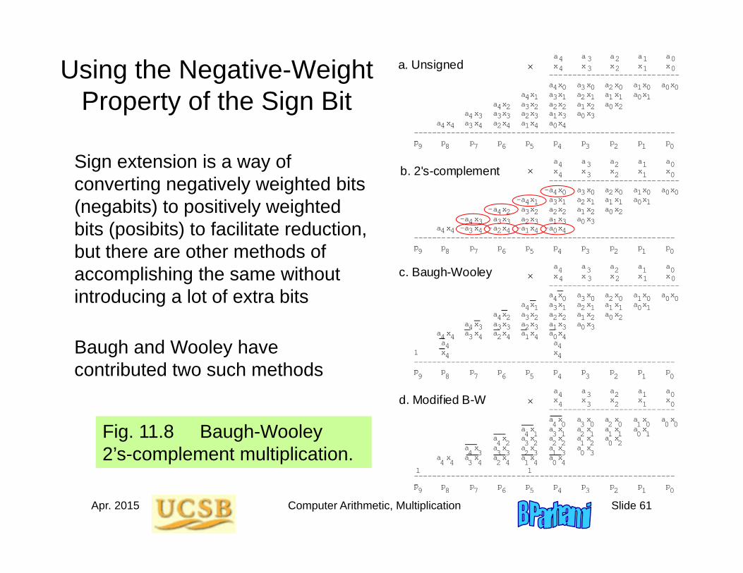
Using the Negative-Weight Property of the Sign Bit

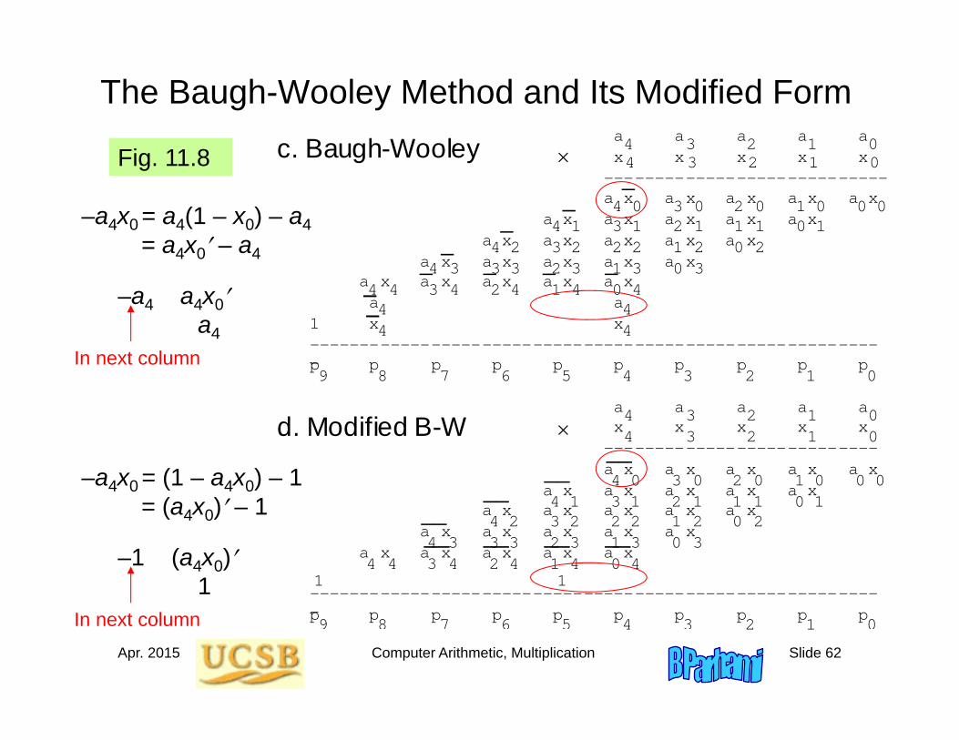
Fig. 11.8 Baugh-Wooley 2’s-complement multiplication.

Sign extension is a way of converting negatively weighted bits (negabits) to positively weighted bits (posibits) to facilitate reduction, but there are other methods of accomplishing the same without introducing a lot of extra bits

Baugh and Wooley have contributed two such methods

4 3 2 1 0 4 3 2 1 0

4 3 2 1 0 4 3 2 1 0 a x a x a x a x a x

a a a a a x x x x x 4 0 3 0 2 0 1 0 0 0 4 1 3 1 2 1 1 1 0 1 4 2 3 2 2 2 1 2 0 2 4 3 3 3 2 3 1 3 0 3 4 4 3 4 2 4 1 4 0 4

a a a a a x x x x x ---------------------------- a x a x a x a x a x a x a x a x a x a x a x a x a x a x a x a x a x a x a x a x a x a x a x a x a x --------------------------------------------------------- p p p p p p p p p p a a a a a x x x x x ---------------------------- -a x a x a x a x a x -a x a x a x a x a x -a x a x a x a x a x -a x a x a x a x a x a x -a x -a x -a x -a x --------------------------------------------------------- p p p p p p p p p p a a a a a x x x x x ---------------------------- a x a x a x a x a x a x a x a x a x a x a x a x a x a x a x a x a x a x a x a x a x a x a x a x a x a a 1 x x --------------------------------------------------------- p p p p p p p p p p --------------------------- a x a x a x a x a x a x a x a x a x a x a x a x a x a x a x a x a x a x a x a x --------------------------------------------------------- p p p p p p p p p p

1 1

4 0 3 0 2 0 1 0 0 0 4 1 3 1 2 1 1 1 0 1 4 2 3 2 2 2 1 2 0 2 4 3 3 3 2 3 1 3 0 3 4 4 3 4 2 4 1 4 0 4 4 4 4 4

4 3 2 1 0 4 3 2 1 0

4 3 2 1 0 4 3 2 1 0

4 0 3 0 2 0 1 0 0 0 4 1 3 1 2 1 1 1 0 1 4 2 3 2 2 2 1 2 0 2 4 3 3 3 2 3 1 3 0 3 4 4 3 4 2 4 1 4 0 4

4 0 3 0 2 0 1 0 0 0 4 1 3 1 2 1 1 1 0 1 4 2 3 2 2 2 1 2 0 2 4 3 3 3 2 3 1 3 0 3 4 4 3 4 2 4 1 4 0 4

9 8 7 6 5 4 3 2 1 0

9 8 7 6 5 4 3 2 1 0

9 8 7 6 5 4 3 2 1 0

9 8 7 6 5 4 3 2 1 0

a. Unsigned

b. 2's-complement

c. Baugh-Wooley

d. Modified B-W __

__ __

__ __ __ __ __

_ _

_ _

_ _ _ _


Fig. 11.8

4 3 2 1 0 4 3 2 1 0 a x a x a x a x a x

a a a a a x x x x x 4 0 3 0 2 0 1 0 0 0 4 1 3 1 2 1 1 1 0 1 4 2 3 2 2 2 1 2 0 2 4 3 3 3 2 3 1 3 0 3 4 4 3 4 2 4 1 4 0 4

a x -a x -a x -a x -a x --------------------------------------------------------- p p p p p p p p p p a a a a a x x x x x ---------------------------- a x a x a x a x a x a x a x a x a x a x a x a x a x a x a x a x a x a x a x a x a x a x a x a x a x a a 1 x x --------------------------------------------------------- p p p p p p p p p p --------------------------- a x a x a x a x a x a x a x a x a x a x a x a x a x a x a x a x a x a x a x a x --------------------------------------------------------- p p p p p p p p p p

1 1

4 0 3 0 2 0 1 0 0 0 4 1 3 1 2 1 1 1 0 1 4 2 3 2 2 2 1 2 0 2 4 3 3 3 2 3 1 3 0 3 4 4 3 4 2 4 1 4 0 4 4 4 4 4

4 3 2 1 0 4 3 2 1 0

4 4 3 4 2 4 1 4 0 4

9 8 7 6 5 4 3 2 1 0

9 8 7 6 5 4 3 2 1 0

9 8 7 6 5 4 3 2 1 0

c. Baugh-Wooley

d. Modified B-W __

__ __

__ __ __ __ __

_ _

_ _

_ _ _ _

The Baugh-Wooley Method and Its Modified Form

–a4x0 = a4(1 – x0) – a4= a4x0 – a4

–a4 a4x0a4

In next column

–a4x0 = (1 – a4x0) – 1= (a4x0) – 1

–1 (a4x0)1

In next column


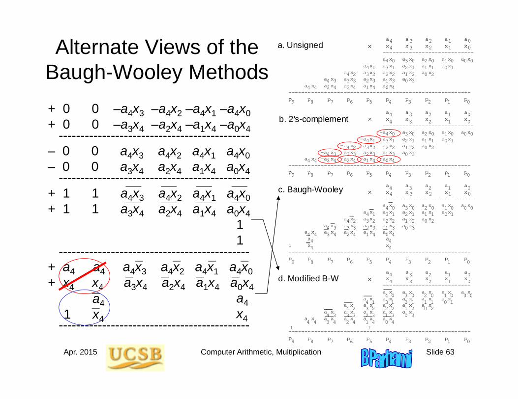
Alternate Views of the Baugh-Wooley Methods+ 0 0 –a4x3 –a4x2 –a4x1 –a4x0+ 0 0 –a3x4 –a2x4 –a1x4 –a0x4--------------------------------------------– 0 0 a4x3 a4x2 a4x1 a4x0– 0 0 a3x4 a2x4 a1x4 a0x4--------------------------------------------+ 1 1 a4x3 a4x2 a4x1 a4x0+ 1 1 a3x4 a2x4 a1x4 a0x4

11

--------------------------------------------+ a4 a4 a4x3 a4x2 a4x1 a4x0+ x4 x4 a3x4 a2x4 a1x4 a0x4

a4x4--------------------------------------------

a41 x4

4 3 2 1 0 4 3 2 1 0

4 3 2 1 0 4 3 2 1 0 a x a x a x a x a x

a a a a a x x x x x 4 0 3 0 2 0 1 0 0 0 4 1 3 1 2 1 1 1 0 1 4 2 3 2 2 2 1 2 0 2 4 3 3 3 2 3 1 3 0 3 4 4 3 4 2 4 1 4 0 4

a a a a a x x x x x ---------------------------- a x a x a x a x a x a x a x a x a x a x a x a x a x a x a x a x a x a x a x a x a x a x a x a x a x --------------------------------------------------------- p p p p p p p p p p a a a a a x x x x x ---------------------------- -a x a x a x a x a x -a x a x a x a x a x -a x a x a x a x a x -a x a x a x a x a x a x -a x -a x -a x -a x --------------------------------------------------------- p p p p p p p p p p a a a a a x x x x x ---------------------------- a x a x a x a x a x a x a x a x a x a x a x a x a x a x a x a x a x a x a x a x a x a x a x a x a x a a 1 x x --------------------------------------------------------- p p p p p p p p p p --------------------------- a x a x a x a x a x a x a x a x a x a x a x a x a x a x a x a x a x a x a x a x --------------------------------------------------------- p p p p p p p p p p

1 1

4 0 3 0 2 0 1 0 0 0 4 1 3 1 2 1 1 1 0 1 4 2 3 2 2 2 1 2 0 2 4 3 3 3 2 3 1 3 0 3 4 4 3 4 2 4 1 4 0 4 4 4 4 4

4 3 2 1 0 4 3 2 1 0

4 3 2 1 0 4 3 2 1 0

4 0 3 0 2 0 1 0 0 0 4 1 3 1 2 1 1 1 0 1 4 2 3 2 2 2 1 2 0 2 4 3 3 3 2 3 1 3 0 3 4 4 3 4 2 4 1 4 0 4

4 0 3 0 2 0 1 0 0 0 4 1 3 1 2 1 1 1 0 1 4 2 3 2 2 2 1 2 0 2 4 3 3 3 2 3 1 3 0 3 4 4 3 4 2 4 1 4 0 4

9 8 7 6 5 4 3 2 1 0

9 8 7 6 5 4 3 2 1 0

9 8 7 6 5 4 3 2 1 0

9 8 7 6 5 4 3 2 1 0

a. Unsigned

b. 2's-complement

c. Baugh-Wooley

d. Modified B-W __

__ __

__ __ __ __ __

_ _

_ _

_ _ _ _


11.4 Partial-Tree and Truncated Multipliers

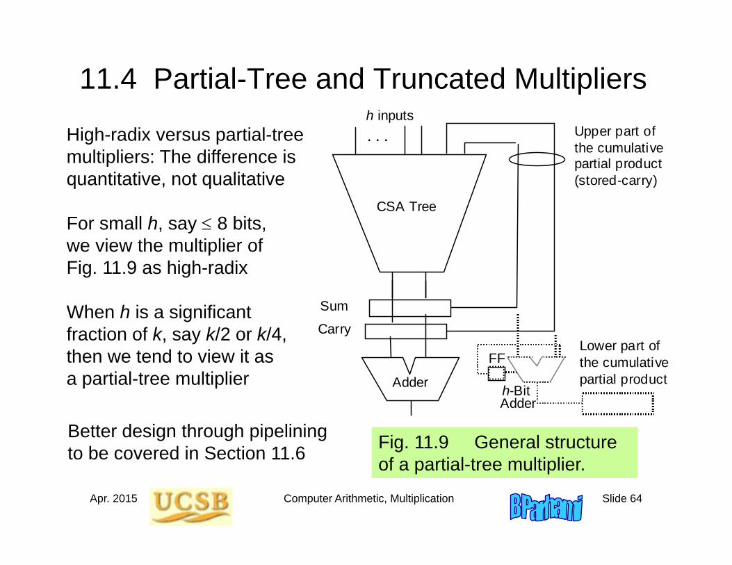
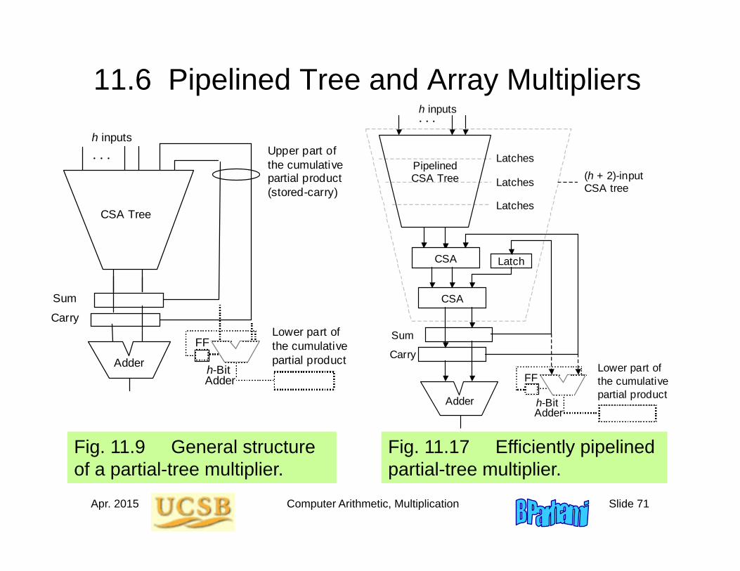
Fig. 11.9 General structure of a partial-tree multiplier.

. . .

CSA Tree

h inputs

Adder

Lower part of the cumulative partial product

FF

h-Bit Adder

Sum Carry

Upper part of the cumulative partial product (stored-carry)

High-radix versus partial-tree multipliers: The difference is quantitative, not qualitative

For small h, say 8 bits, we view the multiplier of Fig. 11.9 as high-radix

When h is a significant fraction of k, say k/2 or k/4,then we tend to view it as a partial-tree multiplier

Better design through pipelining to be covered in Section 11.6


Why Truncated Multipliers?

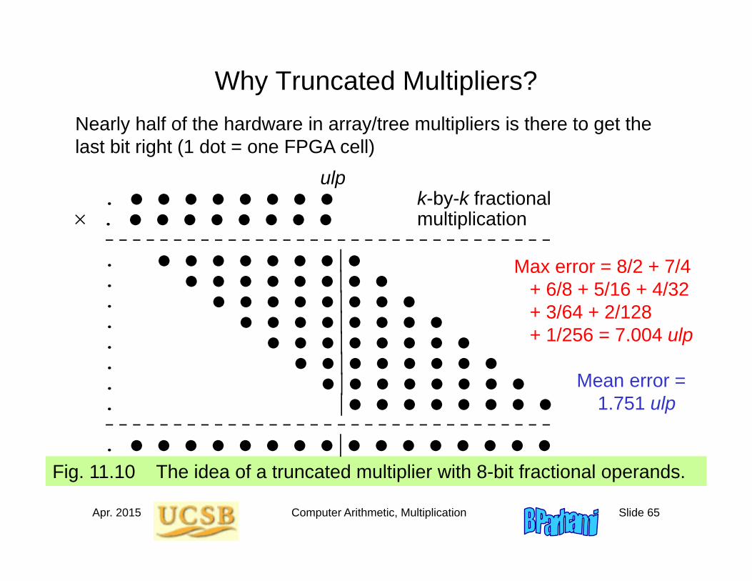
Fig. 11.10 The idea of a truncated multiplier with 8-bit fractional operands.

Nearly half of the hardware in array/tree multipliers is there to get the last bit right (1 dot = one FPGA cell)

ulp. k-by-k fractional

. multiplication---------------------------------. |. |

. |

. |

. |

. |

. |

. |

---------------------------------. |

Max error = 8/2 + 7/4 + 6/8 + 5/16 + 4/32 + 3/64 + 2/128 + 1/256 = 7.004 ulp

Mean error = 1.751 ulp


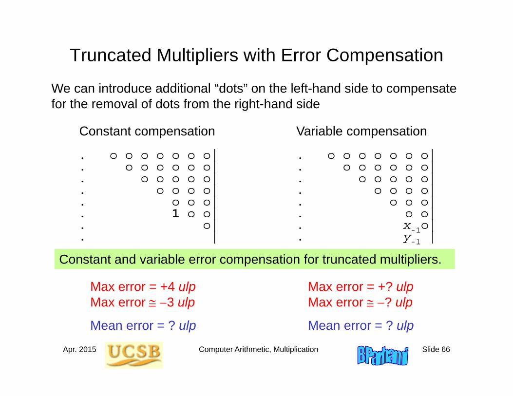
Truncated Multipliers with Error Compensation

Constant and variable error compensation for truncated multipliers.

We can introduce additional “dots” on the left-hand side to compensate for the removal of dots from the right-hand side

Constant compensation Variable compensation

. o o o o o o o| . o o o o o o o|

. o o o o o o| . o o o o o o|

. o o o o o| . o o o o o|

. o o o o| . o o o o|

. o o o| . o o o|

. 1 o o| . o o|

. o| . x-1o|

. | . y-1 |

Max error = +4 ulpMax error 3 ulp

Max error = +? ulpMax error ? ulp

Mean error = ? ulp Mean error = ? ulp


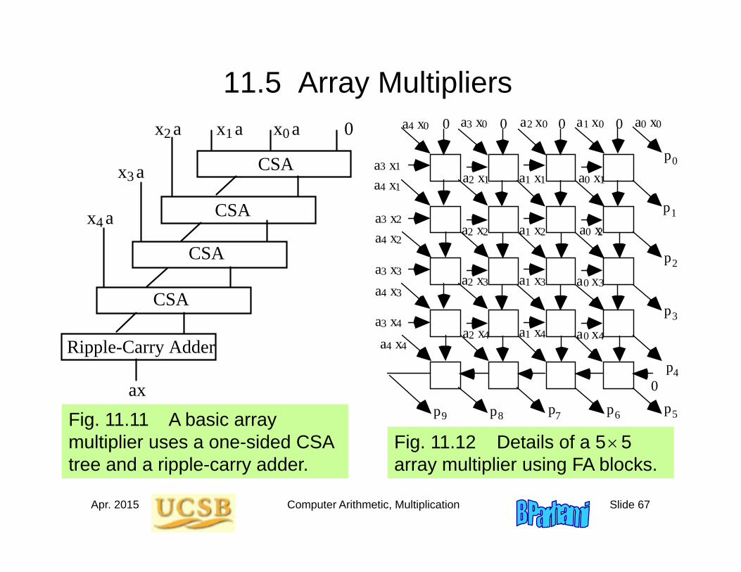
11.5 Array Multipliers

Fig. 11.11 A basic array multiplier uses a one-sided CSA tree and a ripple-carry adder.

0x ax ax a

x a

x a

CSA

CSA

CSA

CSA

Ripple-Carry Adder

012

3

4

ax

p

0

p

1

p

2

p

3

p

4

p 6 p 7 p 8

a x

0 0

a x

1 0

a x

2 0

a x

3 0

a x

4 0

0

0

0

0

a x

0 1

a x

1 1

a x

2 1

a x

3 1

p 9 p 5

a x

4 1

a x

4 2

a x

4 3

a x

4 4

a x

0 2

a x

1 2

a x

2 2

a x

3 2

a x

0 3

a x

1 3

a x

2 3

a x

3 3

a x

0 4

a x

1 4

a x

2 4

a x

3 4

0

Fig. 11.12 Details of a 55 array multiplier using FA blocks.


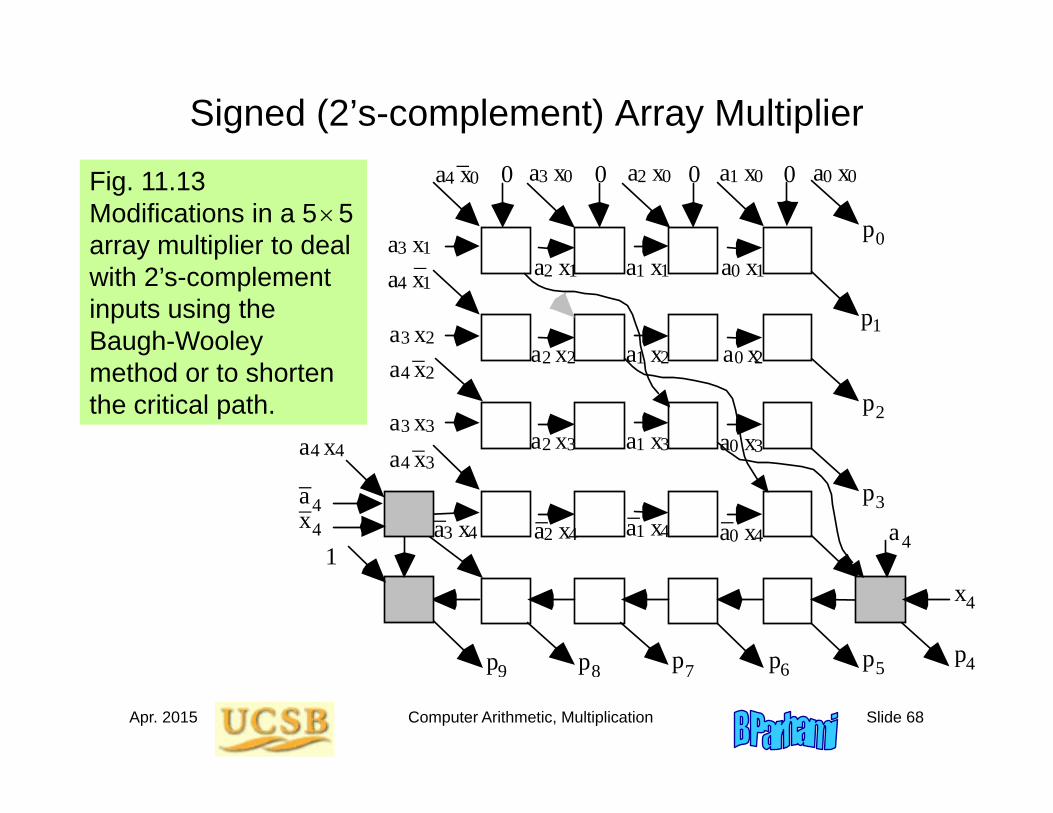
Signed (2’s-complement) Array Multiplier

Fig. 11.13 Modifications in a 55 array multiplier to deal with 2’s-complement inputs using the Baugh-Wooley method or to shorten the critical path.

p

0

p

1

p

2

p

3

p 4 p 6p 7p 8

a x

0 0

a x

1 0

a x

2 0

a x

3 0

a x

4 0

0

0

0

0

a x

0 1

a x

1 1

a x

2 1

a x

3 1

p 9 p 5

a x

4 1

a x

4 2

a x

4 3

a x

4 4

a x

0 2

a x

1 2

a x

2 2

a x

3 2

a x

0 3

a x

1 3

a x

2 3

a x

3 3

a x

0 4

a x

1 4

a x

2 4

a x

3 4 1

x

4

a

4

a

4 x

4

_

_

_

_

_

_

_

_

_

_


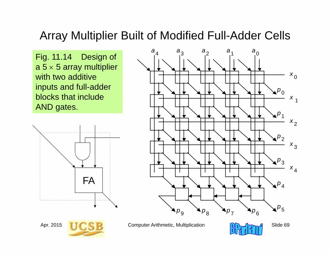
Array Multiplier Built of Modified Full-Adder Cells

Fig. 11.14 Design of a 5 5 array multiplier with two additive inputs and full-adder blocks that include AND gates.

p p p p p

4 3 2 1 0 a a a a a

4

3

2

1

0

x

x

x

x

x

4

3

2

1

0

p

p

p

p

p

9 8 7 6 5

FA


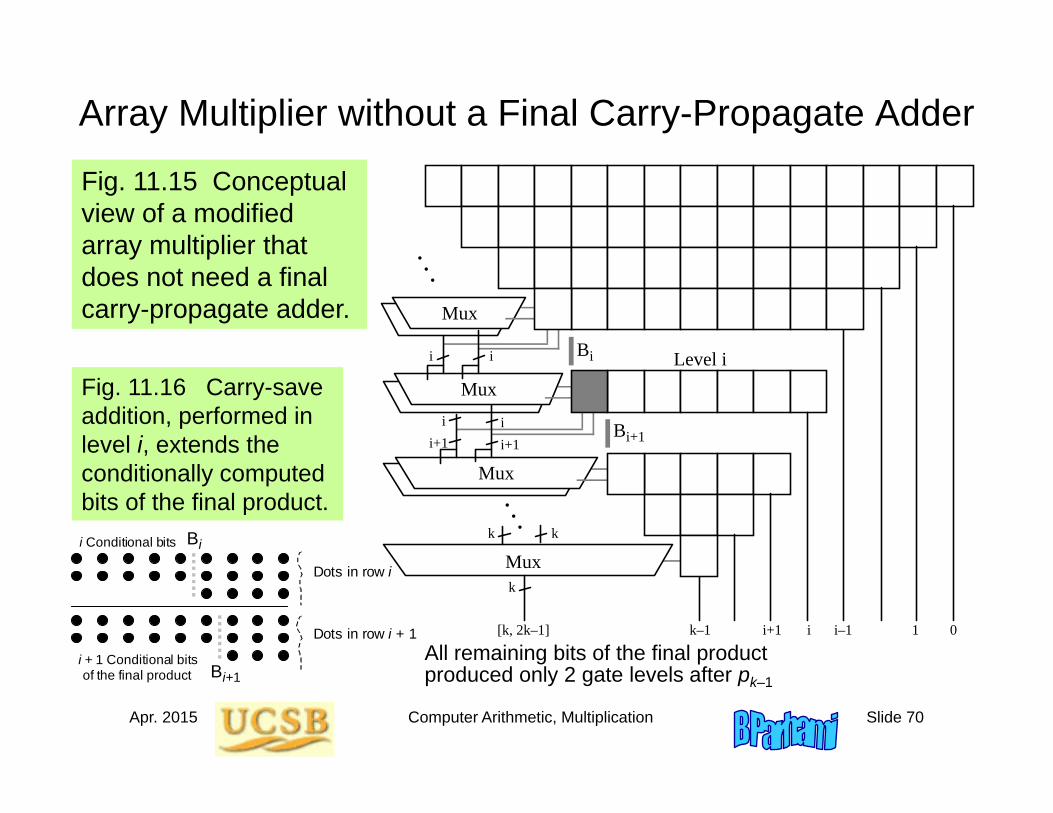
Array Multiplier without a Final Carry-Propagate Adder

Fig. 11.15 Conceptual view of a modified array multiplier that does not need a final carry-propagate adder.

i+1i

i+1i

i i

Mux

Mux

Muxk

[k, 2k–1] 1i–1ii+1k–1

Level i

k k

0

Mux

...

...

Bi+1

Bi

Dots in row i + 1

B

i

B i+1

Dots in row i

i Conditional bits

i + 1 Conditional bits of the final product

Fig. 11.16 Carry-save addition, performed in level i, extends the conditionally computed bits of the final product.

All remaining bits of the final product produced only 2 gate levels after pk–1


11.6 Pipelined Tree and Array Multipliers

. . .

CSA Tree

h inputs

Adder


FF

h-Bit Adder

Sum Carry

Upper part of the cumulative partial product (stored-carry)

Fig. 11.9 General structure of a partial-tree multiplier.

Fig. 11.17 Efficiently pipelined partial-tree multiplier.

. . .

h inputs

Adder


FF

h-Bit Adder

Sum Carry

CSA

Pipelined CSA Tree

Latches Latches Latches

CSA

(h + 2)-input CSA tree

Latch


Pipelined Array Multipliers

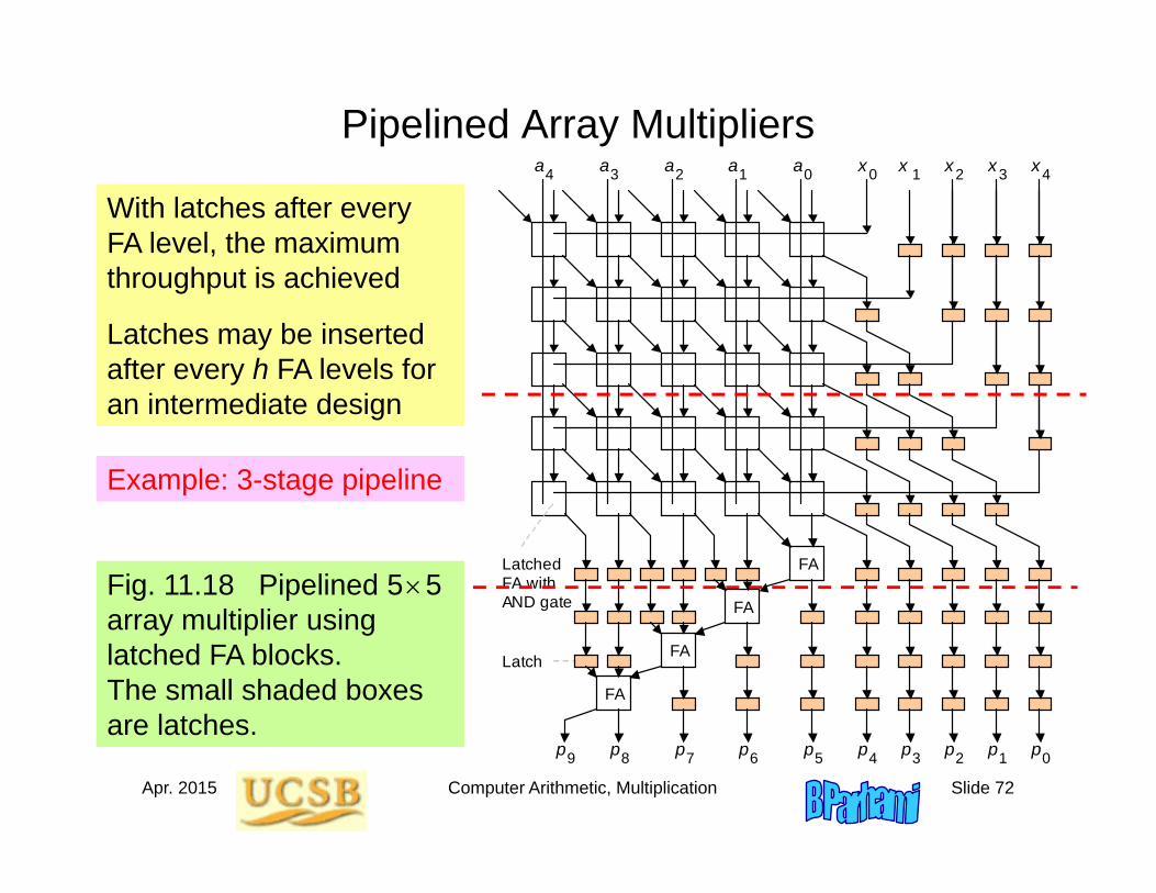
With latches after every FA level, the maximum throughput is achieved

Latches may be inserted after every h FA levels for an intermediate design

Fig. 11.18 Pipelined 55 array multiplier using latched FA blocks. The small shaded boxes are latches.

p p p p p

4 3 2 1 0 a a a a a 4 3 2 1 0 xxxxx

4 3 2 1 0 p p p p p 9 8 7 6 5

Latched FA with AND gate

Latch

FA

FA

FA

FA

Example: 3-stage pipeline


12 Variations in Multipliers

Chapter GoalsLearn additional methods for synthesizingfast multipliers as well as other typesof multipliers (bit-serial, modular, etc.)

Chapter HighlightsBuilding a multiplier from smaller unitsPerforming multiply-add as one operationBit-serial and (semi)systolic multipliersUsing a multiplier for squaring is wasteful


Variations in Multipliers: Topics


12.1 Divide-and-Conquer Designs

12.2 Additive Multiply Modules

12.3 Bit-Serial Multipliers

12.4 Modular Multipliers

12.5 The Special Case of Squaring

12.6 Combined Multiply-Add Units


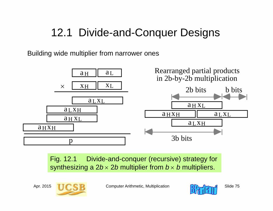
12.1 Divide-and-Conquer Designs

Building wide multiplier from narrower ones

Fig. 12.1 Divide-and-conquer (recursive) strategy for synthesizing a 2b 2b multiplier from b b multipliers.

a

p

Rearranged partial products in 2b-by-2b multiplication

2b bits

3b bits

H a L

xH xL

a L xH

a L xL

a H xLxHa H

a H xL

a L xH

a L xLxHa H

b bits


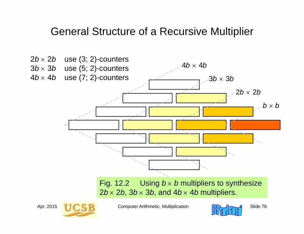
General Structure of a Recursive Multiplier

2b 2b use (3; 2)-counters3b 3b use (5; 2)-counters4b 4b use (7; 2)-counters

Fig. 12.2 Using b b multipliers to synthesize 2b 2b, 3b 3b, and 4b 4b multipliers.

4b 4b

3b 3b

2b 2b

b b


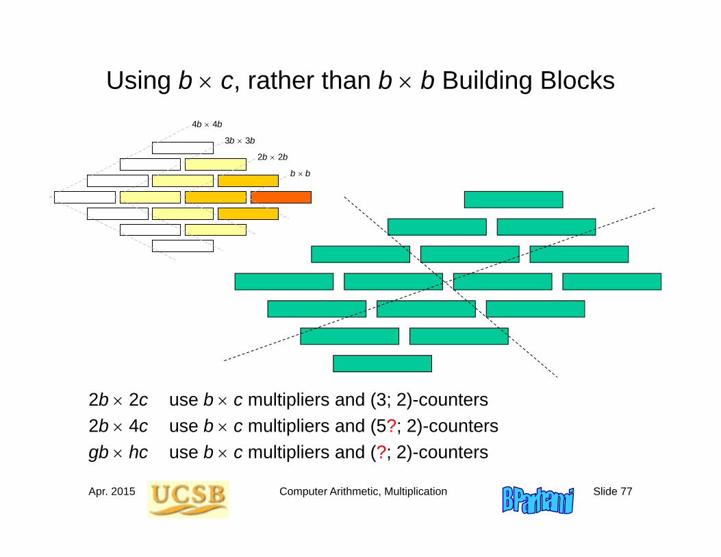
Using b c, rather than b b Building Blocks

2b 2c use b c multipliers and (3; 2)-counters2b 4c use b c multipliers and (5?; 2)-countersgb hc use b c multipliers and (?; 2)-counters

4b 4b

3b 3b

2b 2b

b b


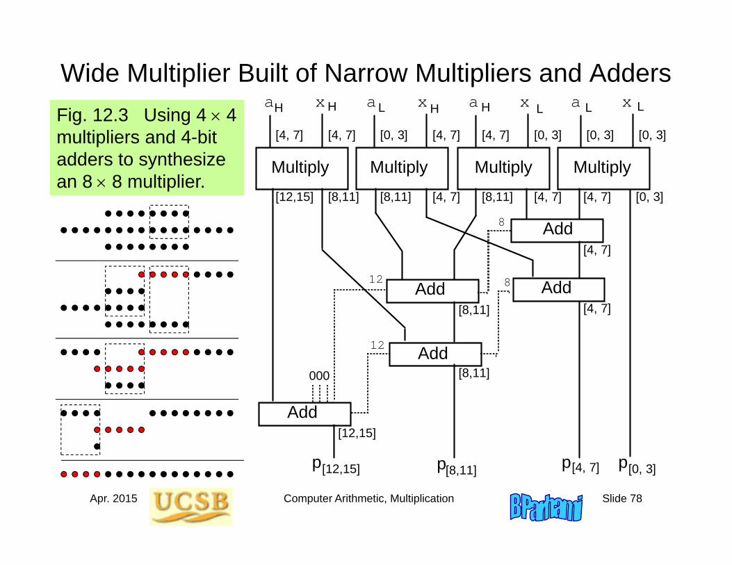
Wide Multiplier Built of Narrow Multipliers and AddersFig. 12.3 Using 4 4 multipliers and 4-bit adders to synthesize an 8 8 multiplier.

a x a x a x a x

Add

Add

Add

Add Add

pp p p

000

8

8

12

12

H LH H H LLL

[4, 7] [4, 7] [0, 3] [4, 7] [4, 7] [0, 3] [0, 3] [0, 3]

[12,15] [8,11] [8,11] [4, 7] [8,11] [4, 7] [4, 7] [0, 3]

[4, 7]

[4, 7]

[8,11]

[8,11]

[12,15]

[12,15] [8,11] [0, 3][4, 7]

Multiply MultiplyMultiplyMultiply


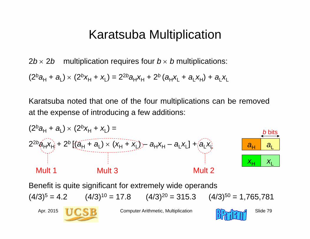
Karatsuba Multiplication

2b 2b multiplication requires four b b multiplications:

(2baH + aL) (2bxH + xL) = 22baHxH + 2b (aHxL + aLxH) + aLxL

aH aL

xH xL

Karatsuba noted that one of the four multiplications can be removedat the expense of introducing a few additions:

(2baH + aL) (2bxH + xL) =

22baHxH + 2b [(aH + aL) (xH + xL) – aHxH – aLxL] + aLxL

Mult 1 Mult 2Mult 3

Benefit is quite significant for extremely wide operands(4/3)5 = 4.2 (4/3)10 = 17.8 (4/3)20 = 315.3 (4/3)50 = 1,765,781

b bits


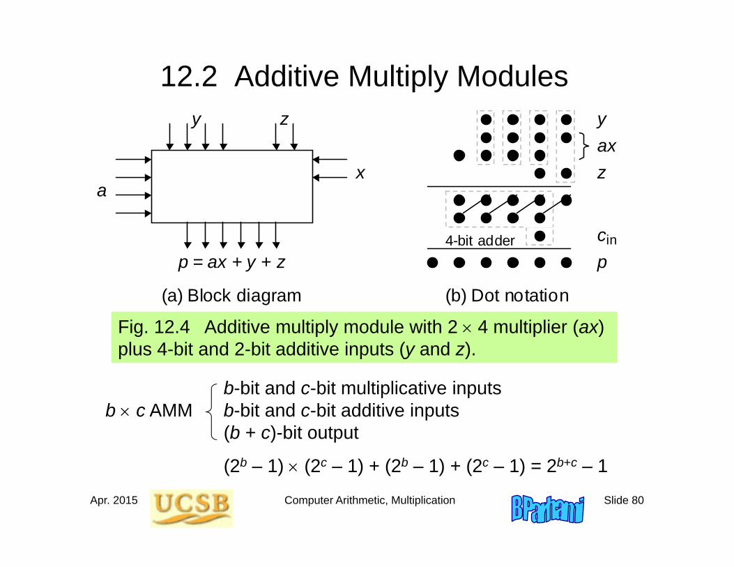
12.2 Additive Multiply Modules

Fig. 12.4 Additive multiply module with 2 4 multiplier (ax) plus 4-bit and 2-bit additive inputs (y and z).

c

in

y

z

ax

p

4-bit adder

y

z

x a

p = ax + y + z

(a) Block diagram (b) Dot notation

b-bit and c-bit multiplicative inputsb c AMM b-bit and c-bit additive inputs

(b + c)-bit output

(2b – 1) (2c – 1) + (2b – 1) + (2c – 1) = 2b+c – 1


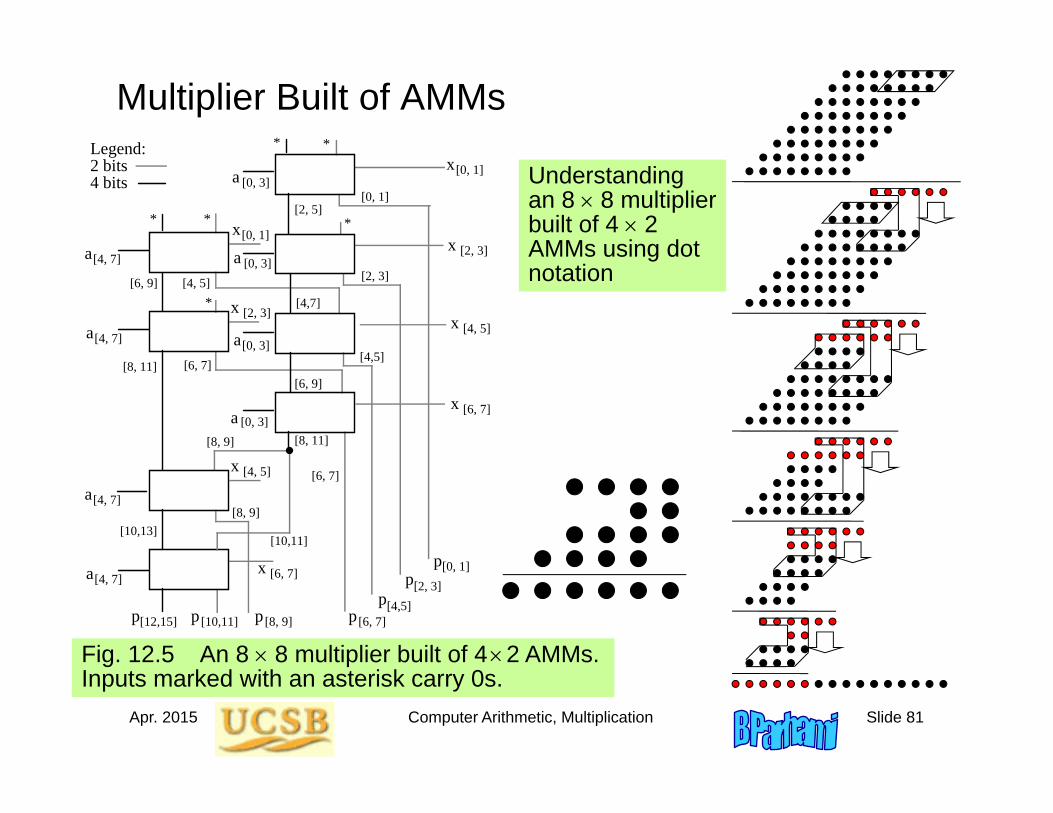
Multiplier Built of AMMs

Fig. 12.5 An 8 8 multiplier built of 42 AMMs. Inputs marked with an asterisk carry 0s.

[0, 1]

[2, 3]

[4, 5]

[6, 7]

[8, 9][10,11][12,15]

[0, 1][2, 3]

[4,5][6, 7]

x

x

x

x [0, 3]a

[0, 3]a

[0, 3]a

[0, 3]a

p

pp

pppp

[0, 1]x

[2, 3]

[4, 5]

[6, 7]x

x

x

[10,11]

[8, 9]

[4, 7]a

[4, 7]a

[4, 7]a

[4, 7]a

[8, 9]

[0, 1]

[2, 3][4, 5]

[6, 7][4,5]

[6, 7]

[8, 11]

[10,13]

[2, 5]

[4,7]

[6, 9][8, 11]

[6, 9]

*

*

* *

**

Legend: 2 bits 4 bits Understanding

an 8 8 multiplier built of 4 2 AMMs using dot notation


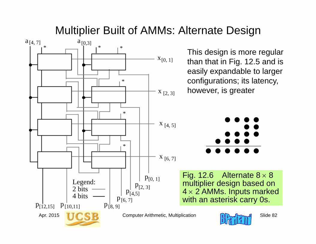
Multiplier Built of AMMs: Alternate Design

Fig. 12.6 Alternate 8 8 multiplier design based on 4 2 AMMs. Inputs marked with an asterisk carry 0s.

[8, 9]p

* *

*

*

*

*

[0, 1]

[2, 3]

[4, 5]

[6, 7]

x

x

x

x

[10,11][12,15]

[0, 1][2, 3]

[4,5][6, 7]

p

pp

pp

p

[0,3] [4, 7] aa

Legend: 2 bits 4 bits

This design is more regular than that in Fig. 12.5 and is easily expandable to larger configurations; its latency, however, is greater


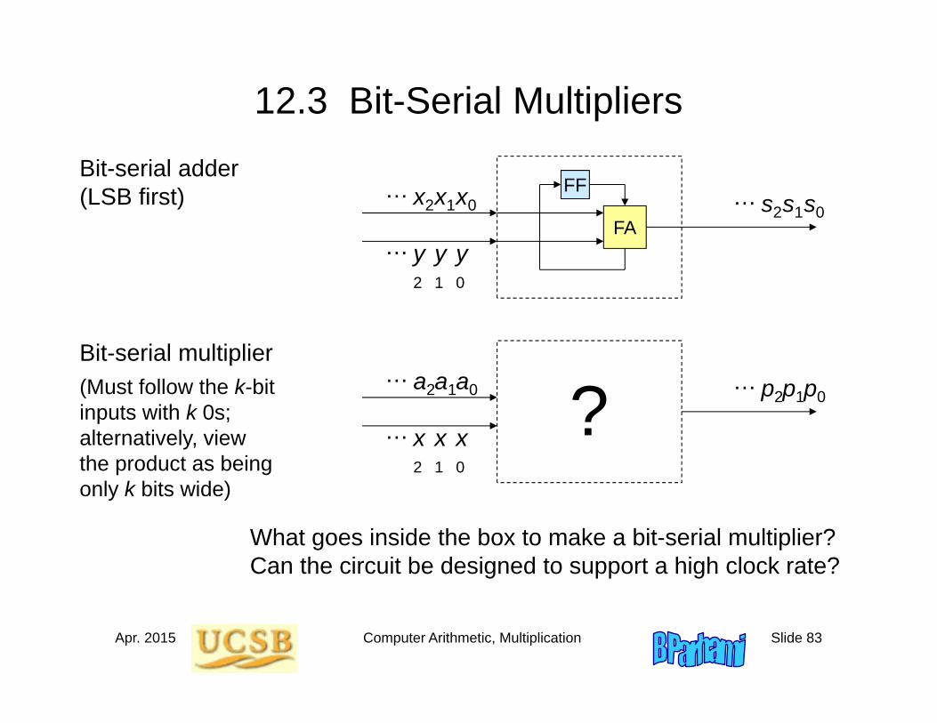
12.3 Bit-Serial Multipliers

What goes inside the box to make a bit-serial multiplier?Can the circuit be designed to support a high clock rate?

FA

FFBit-serial adder(LSB first) x0

y0

s0x1

y1

s1x2

y2

s2…

…

…

Bit-serial multipliera1

x1

p1a0

x0

p0a2

x2

p2…

…

…(Must follow the k-bit inputs with k 0s; alternatively, view the product as being only k bits wide)

?


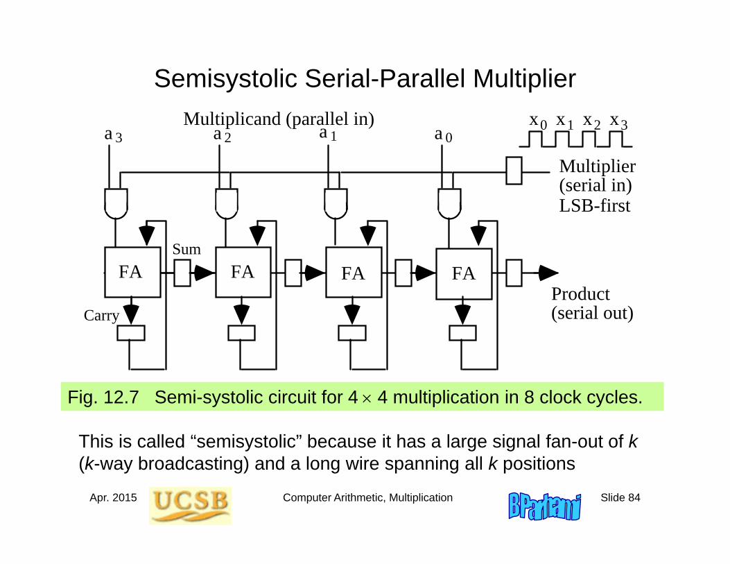
Semisystolic Serial-Parallel MultiplierMultiplicand (parallel in)

Multiplier (serial in)LSB-first

Carry

SumFA

Product (serial out)

FA FA FA

a 3 a 2 a 1 a 0x0 x1 x2 x3

Fig. 12.7 Semi-systolic circuit for 4 4 multiplication in 8 clock cycles.

This is called “semisystolic” because it has a large signal fan-out of k(k-way broadcasting) and a long wire spanning all k positions


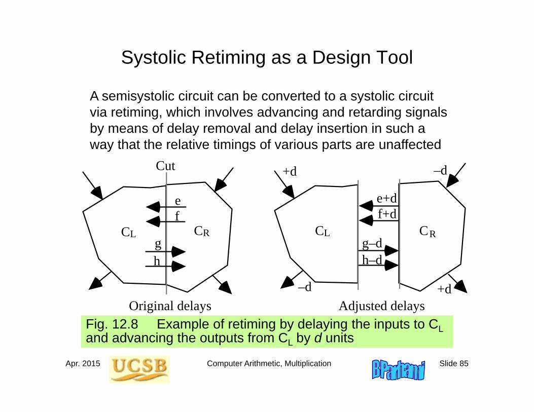
Systolic Retiming as a Design Tool

Fig. 12.8 Example of retiming by delaying the inputs to CLand advancing the outputs from CL by d units

Cut

CL CR CL CR

ef

gh

e+df+d

g–dh–d

+d

–d

–d

+dOriginal delays Adjusted delays

A semisystolic circuit can be converted to a systolic circuit via retiming, which involves advancing and retarding signals by means of delay removal and delay insertion in such a way that the relative timings of various parts are unaffected


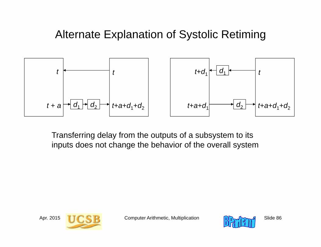
Alternate Explanation of Systolic Retiming

Transferring delay from the outputs of a subsystem to its inputs does not change the behavior of the overall system

td1

d2 t+a+d1+d2

t+d1

t+a+d1

tt

t + a d1 d2 t+a+d1+d2


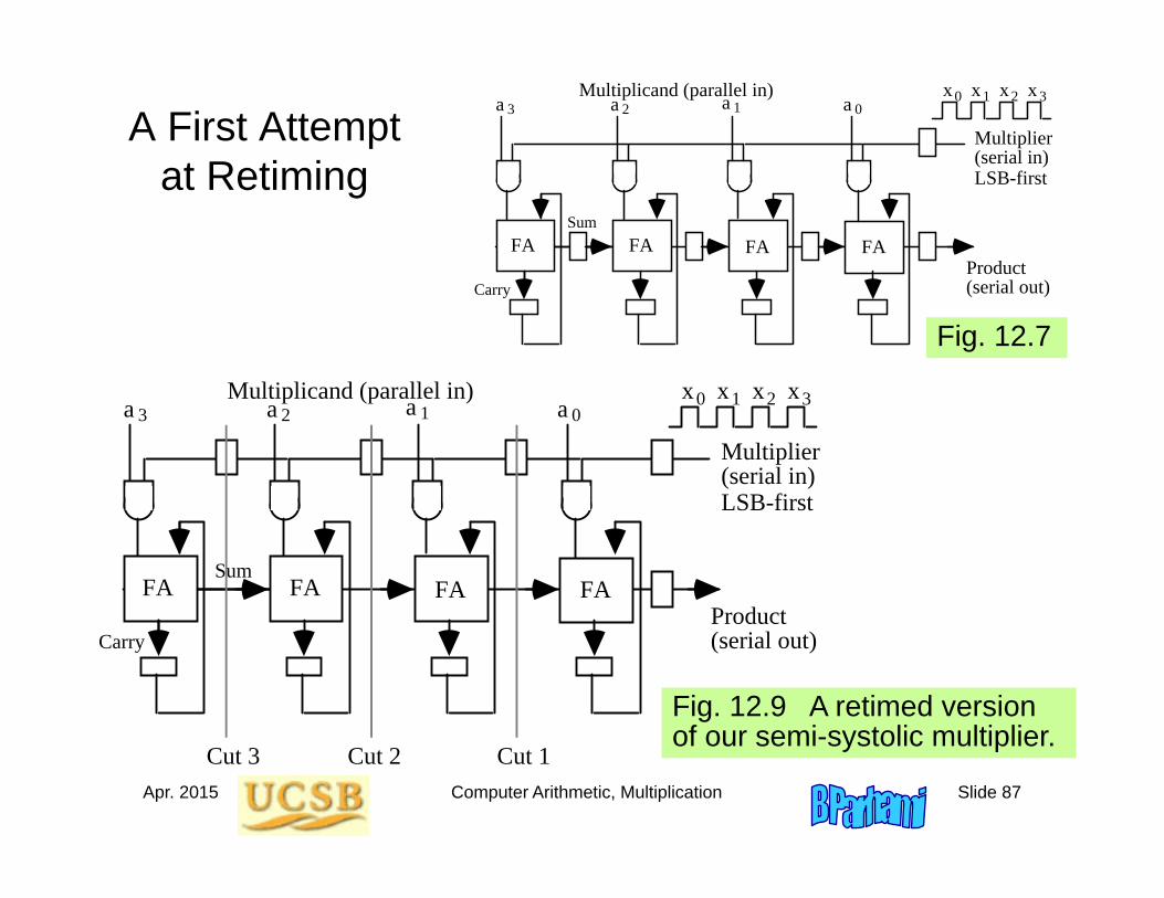
A First Attempt at Retiming

Fig. 12.9 A retimed version of our semi-systolic multiplier.

Multiplicand (parallel in)


Carry

FAProduct (serial out)

FA FA FA

a 3 a 2 a 1 a 0x0 x1 x2 x3

Sum

Cut 1Cut 2Cut 3



Carry

SumFA


FA FA FA

a 3 a 2 a 1 a 0x0 x1 x2 x3

Fig. 12.7


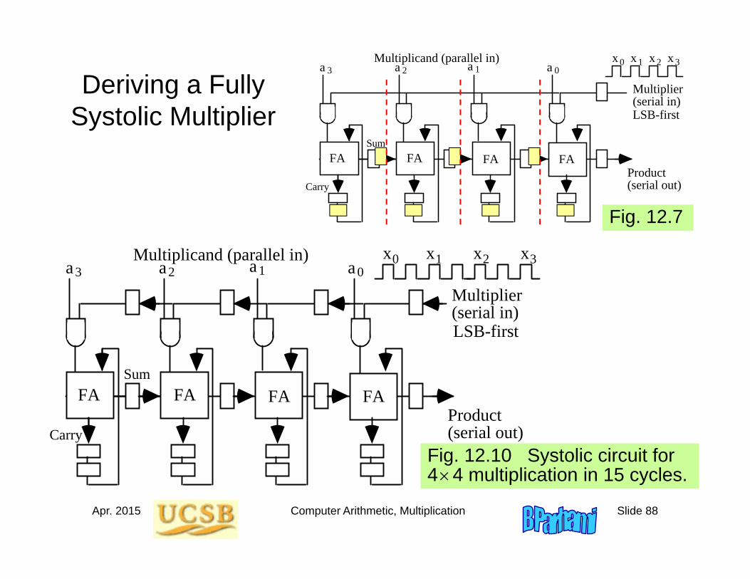
Deriving a Fully Systolic Multiplier



Carry

SumFA


FA FA FA

a 3 a 2 a 1 a 0x 0 x 1 x 2 x 3

Fig. 12.7

Fig. 12.10 Systolic circuit for 44 multiplication in 15 cycles.



SumFA


FA FA FA

a3 a2 a1 a0x0 x1 x2 x3

Carry


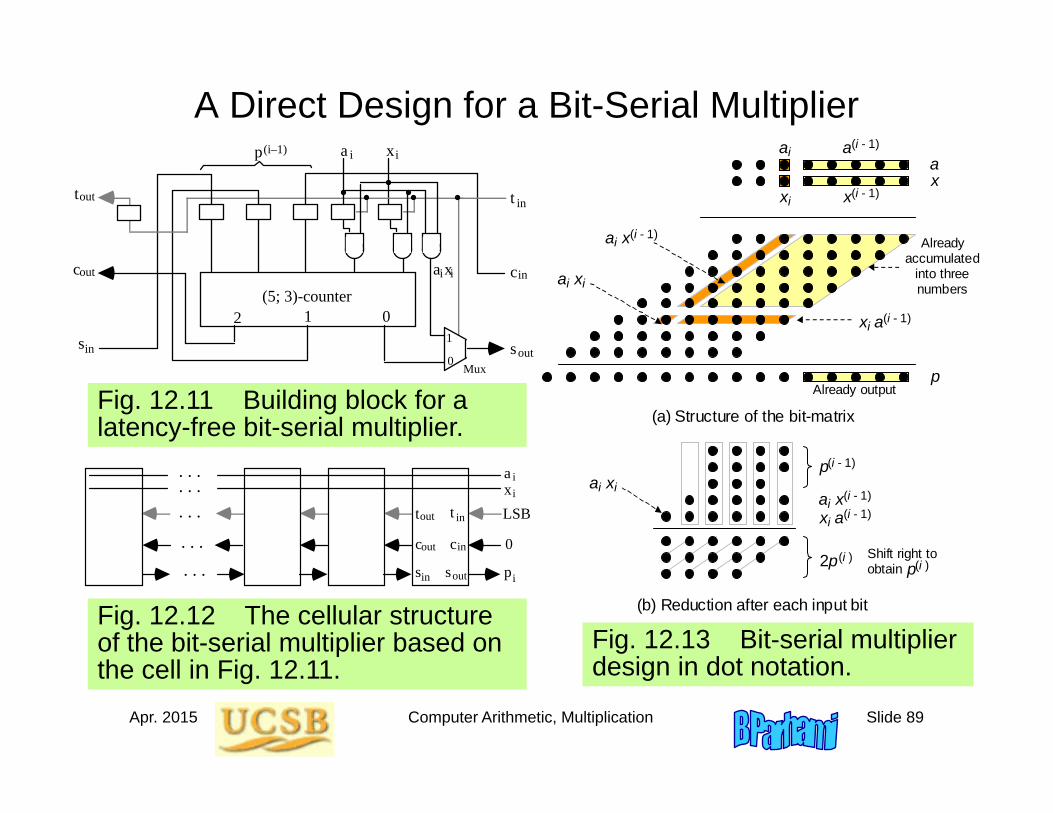
A Direct Design for a Bit-Serial Multiplier

Fig. 12.13 Bit-serial multiplier design in dot notation.

p

x

a

Already accumulated

into three numbers

(i - 1)

a

x

(i - 1)

i

a

x

i

x

i

(i - 1)

a

i

a

x

(i - 1)

x

i

i

a

Already output

(a) Structure of the bit-matrix

(b) Reduction after each input bit

p

(i - 1)

i

a

x

(i - 1)

x

i

(i - 1)

a

x

i

i

a

2p

(i )

Shift right to obtain p

(i )

Mux

(5; 3)-counter

0

1

012

a x

a x

ss

c c

t t in

out in

in out

out

p

ii

ii(i–1)

ax

ss

c c

t t in

out in

in out

out

p

ii

. . .. . .

. . .

. . .

. . .

i

LSB

0

Fig. 12.11 Building block for a latency-free bit-serial multiplier.

Fig. 12.12 The cellular structure of the bit-serial multiplier based on the cell in Fig. 12.11.


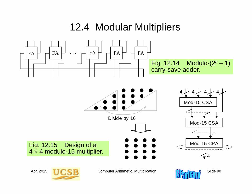
12.4 Modular Multipliers

. . .FA FAFAFAFA

Mod-15 CSA

Divide by 16

4

4

4

4

Mod-15 CSA

4

Mod-15 CPA

Fig. 12.14 Modulo-(2b – 1) carry-save adder.

Fig. 12.15 Design of a 4 4 modulo-15 multiplier.


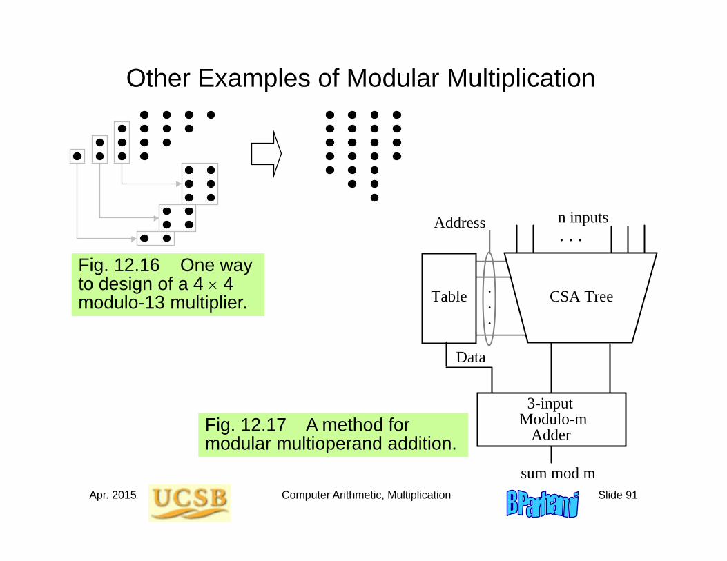
Other Examples of Modular Multiplication

Fig. 12.16 One way to design of a 4 4 modulo-13 multiplier.

Fig. 12.17 A method for modular multioperand addition.

. . .

Table

n inputs

CSA Tree

sum mod m

3-input Modulo-m Adder

.

.

.

Address

Data


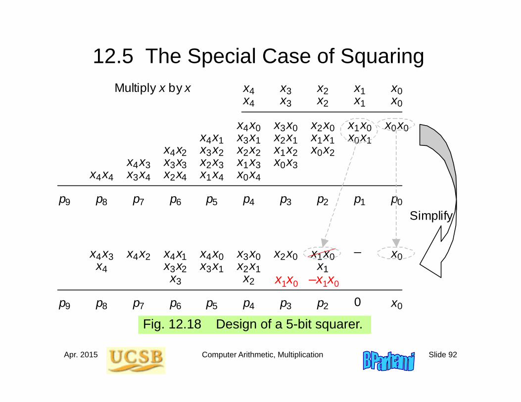
12.5 The Special Case of Squaringx 0 x 1 x 2 x 3 x 4 x 0 x 1 x 2 x 3 x 4

x 0 x 1 x 2 x 3 x 4 x 0 x 0

p 0

x 4

x 1

x 4

x 0 x 1

x 2 x 3

x 4

x 0 x 1

x 2 x 3

x 4

x 0

Multiply x by x

x 1 x 2 x 3 x 4 x 0 x 1 x 2 x 3 x 4 x 0

x 1 x 2 x 3 x 4 x 0 x 1 x 2 x 3 x 4 x 0

x 1 x 2 x 3

x 1 x 2 x 3

x 2 x 3

x 4

p 1 p 2 p 3 p 4 p 5 p 6 p 7 p 8 p 9

x 1 x 2 x 3 x 4 x 0 x 1

x 0

x 2

x 0 x 1

x 0 x 2 x 3

x 4 x 0 x 3

x 4

x 0

x 1 x 2 x 1

x 2 x 3

x 3 x 4 x 4

p 2 p 3 p 4 p 5 p 6 p 7 p 8 p 9 0

_

Simplify

Fig. 12.18 Design of a 5-bit squarer.

x1x0 –x1x0


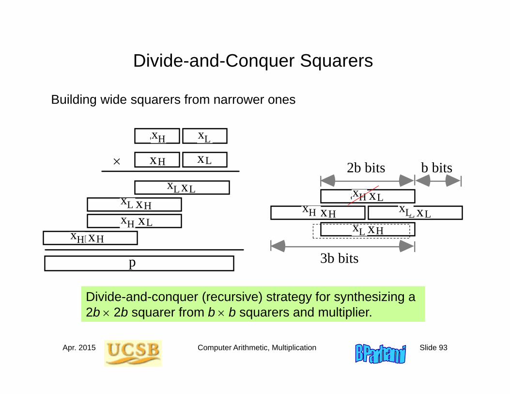
Divide-and-Conquer Squarers

Building wide squarers from narrower ones

Divide-and-conquer (recursive) strategy for synthesizing a 2b 2b squarer from b b squarers and multiplier.

a

p

Rearranged partial products in 2b-by-2b multiplication

2b bits

3b bits

H a L

xH xL

a L xH

a L xL

a H xLxHa H

a H xL

a L xH

a L xLxHa H

b bits

xLxH

xLxL xLxH

xL

xH

xHxH


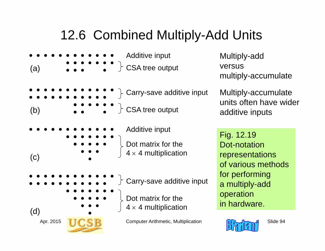
12.6 Combined Multiply-Add Units

Fig. 12.19 Dot-notation representations of various methods for performing a multiply-add operation in hardware.

Multiply-add versus multiply-accumulate

Multiply-accumulate units often have wider additive inputs

(c)

Additive input

Dot matrix for the4 4 multiplication

(a)Additive input

CSA tree output

(b)

Carry-save additive input

CSA tree output

(d)

Carry-save additive input

Dot matrix for the4 4 multiplication

Documents

Part III - Electrical and Computer Engineeringparhami/pres_folder/f31-book-arith-pres... · Basic Addition and Counting Carry-Lookahead Adders ... = p = ax + p(0)2 ... Performing