Embed Size (px)
Citation preview

1
© Michel A. Robe. No part of this primer may be reproduced by or transferred to anyone, in whole or in part, without written prior permission.
Portfolio Management Primer
• Primer I: Top-Down Portfolio Management • Capital vs. Asset allocation• Markowitz security selection model
• Primer II: Asset Pricing Models• CAPM (Theory & Practice)• Index & Multi-Factor Models
• Primer III:• Active Portfolio Management• Performance Measurement: Benchmarks & Rewards
© Michel A. Robe. No part of this primer may be reproduced by or transferred to anyone, in whole or in part, without written prior permission.
Part VI:Active Portfolio
Management

2
© Michel A. Robe. No part of this primer may be reproduced by or transferred to anyone, in whole or in part, without written prior permission.
Active Portfolio Management
• Two examples so far• stocks -- Markowtiz security selection model (need inputs!)• bonds -- fixed-income portfolio management
• Relevant questions• why?
• what? – market timing
– security analysis
» index model» multi-factor model
• how? – key worry = control for risk
© Michel A. Robe. No part of this primer may be reproduced by or transferred to anyone, in whole or in part, without written prior permission.
Active Portfolio Management -- Why?
• APM -- a contradiction in terms?• Nope!
– market efficiency requires many investors to manage actively
• intuitionmis-priced securities
– > deviations from passive strategies pay off– > price pressures eliminate mis-pricing– > active management does not pay off– > securities become mis-priced again– > …
• Theory» Grossman and Stiglitz

3
© Michel A. Robe. No part of this primer may be reproduced by or transferred to anyone, in whole or in part, without written prior permission.
Active Portfolio Management -- Why? 2
• Evidence– other managers may beat the market
» small but statistically significant » noise in security returns −> hard to disclaim
– some portfolio managers are really good » hard to argue
– anomalies» January effect, …
» disappearance?
© Michel A. Robe. No part of this primer may be reproduced by or transferred to anyone, in whole or in part, without written prior permission.
What is Active Portfolio Management?
• Isn’t every strategy active?• 1. Security selection -- clearly
– identify mis-priced securities
• 2. Asset allocation -- yep– different asset categories
» require different forecasts– example
» long-term bond return determinants
» ≠ equity return determinants– international assets
» things get worse

4
© Michel A. Robe. No part of this primer may be reproduced by or transferred to anyone, in whole or in part, without written prior permission.
What is Active Portfolio Management? 2
• Isn’t every strategy active?• 3. capital allocation -- even that!
– proportion invested in market portfolio
– requires to forecast and
– might also lead to market timing
» market conditions change over time
σ 2*
005.02
][
M
fm
xxx A
rrEw
−=
][ mrE σ 2M
© Michel A. Robe. No part of this primer may be reproduced by or transferred to anyone, in whole or in part, without written prior permission.
What is Active Portfolio Management? 3
• Approach• definition
– purely passive strategy » invest only in index funds» one fund per asset category (equity, bonds, bills)» proportions unchanged regardless of market conditions
• example» 60% equity + 30% bonds + 10% bills» fixed for 5 years = entire investment horizon
• active management» requires control of risk

5
© Michel A. Robe. No part of this primer may be reproduced by or transferred to anyone, in whole or in part, without written prior permission.
What is Active Portfolio Management? 4
• Objectives• concentrate on portfolio construction
– CAPM −> we can separate – construction of efficient portfolio– and allocation of funds
» between risky asset and bills
• two components– security analysis
» maximize Sharpe ratio (CAPM)
– market timing» shift assets in and out of risky portfolio
© Michel A. Robe. No part of this primer may be reproduced by or transferred to anyone, in whole or in part, without written prior permission.
Market Timing
• Idea• market timers shift money
» from money market (MM) to risky portfolio
• based on their forecasts of market return
• potential profits• huge• example ($1,000 reinvested from 1927 till 1978)
» 30-day T-bills: $3,600 (r = 2.49%)» NYSE: $ 67,500 (r = 8.44%)» perfect market timing: $5,360,000,000 (r = 34.71%)
• (Tables on p. 985, 6 th edition)

6
© Michel A. Robe. No part of this primer may be reproduced by or transferred to anyone, in whole or in part, without written prior permission.
Market Timing 2
• Reasons for differences• compounding
» for all assets» importance for pension funds
• risk– mainly for equities (Fig. p. 985 6th edition)
» T-bills are mostly risk-free– irrelevant for market timing
» exception: T-bill rate varies a little
• information» for market timing
© Michel A. Robe. No part of this primer may be reproduced by or transferred to anyone, in whole or in part, without written prior permission.
Market Timing 3
• Market timing as an option– much less risky than equities
• standard deviation is misleading– perfect market timing– yields dominant payoffs in each state of the world (Fig. 27.1)
» gives minimum return guarantee
» + a non-negative random number
– market timing fees• market timers will charge for service
» fees determined by option pricing

7
© Michel A. Robe. No part of this primer may be reproduced by or transferred to anyone, in whole or in part, without written prior permission.
Market Timing 4
• In practice• clients
– want managers to pick efficient portfolios» maximize Sharpe ratio
– still need to pick the optimal proportion» to invest in the risk-free asset
• managers– need to update customers continuously
» relative attractiveness of risky portolio changes– costly
• solution– let managers shift money in and out of MM funds
» = solution used by most funds
© Michel A. Robe. No part of this primer may be reproduced by or transferred to anyone, in whole or in part, without written prior permission.
Market Timing 5
• Evaluating market timers• Basic idea
– Risk-return trade-off (Q1c, Assignment 2)– fund performance should improve with the market
• Intuition– as market improves,
a good market timer shifts more money to market
» caveat: true if short sales are ruled out
• Formally– Non-linear regressions (Fig. 24.5, BKM6)
» Regress portfolio excess returns (ER) on market ER and ER^2

8
© Michel A. Robe. No part of this primer may be reproduced by or transferred to anyone, in whole or in part, without written prior permission.
Security Selection
• Map• A. idea
• B. portfolio construction
• C. numerical example
• D. multi- factor models
• E. use in practice» industry use
» advantages vs. dangers
© Michel A. Robe. No part of this primer may be reproduced by or transferred to anyone, in whole or in part, without written prior permission.
Security Selection 2
• A. Idea (Treynor-Black)• 1. consider the entire set of securities
» assume the entire set is there» index model (passive portfolio = market porfolio)
• 2. focus on a small subset» as many as analysts can reasonably handle
• 3. analyze– use index (single - or multi-) factor model
» to estimate alpha, beta(s) and residual risk» of securities in subset
– identify securities with positive expected “alpha”» assume securities outside the subset are correctly priced

9
© Michel A. Robe. No part of this primer may be reproduced by or transferred to anyone, in whole or in part, without written prior permission.
Security Selection 3
• A. (continued)• 4. mix non-zero alpha securities
» with passive portfolio (= market porfolio)
– why?
» want to maximize return» but need to control for risk» small subset −> too much risk if invest only in subset
– how?
» use the beta, alpha and residual risk estimated
• 5. optimal risky portfolio» = mix of active and passive portfolio
© Michel A. Robe. No part of this primer may be reproduced by or transferred to anyone, in whole or in part, without written prior permission.
Security Selection 4
• B. Portfolio construction (NOT Exam Mat’l)• 1. assumptions (index model)
– market portfolio M = efficient portfolio
– and have been estimated
» use them for passive portfolio» no need for market timing
– beta relationship
][ mrE σ 2M
ifMiifi errrr +−+=− )(βα
0),cov(),cov( == Miji reee

10
© Michel A. Robe. No part of this primer may be reproduced by or transferred to anyone, in whole or in part, without written prior permission.
Security Selection 5
• B. (continued)• 2. research or estimate
• 3. active portfolio» −> done (i.e., keep security in passive portf.)
» −> go long
» −> go short
» optimal weights:
kkfMkfk errrr αβ ++−+= )(
0=kα0>kα
0<kα
∑=
= n
jjj
kkk
e
ew
12
2
)(/
)(/
σα
σα1
1=∑
=
n
kkw
© Michel A. Robe. No part of this primer may be reproduced by or transferred to anyone, in whole or in part, without written prior permission.
Security Selection 6
• B. (continued)• active portfolio
» “A” comprises all the assets with non-zero alpha
∑=
=n
kkkA w
1αα ∑
==
n
kkkA w
1ββ
)(2222AMAA eσσβσ +=
∑=
+=n
kkkMA ew
1
2222 )(σσβ 0),cov( =ji ee
11
© Michel A. Robe. No part of this primer may be reproduced by or transferred to anyone, in whole or in part, without written prior permission.
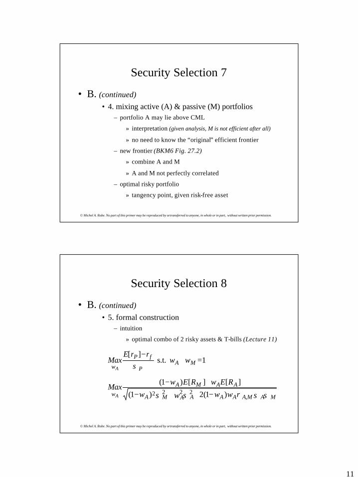
Security Selection 7
• B. (continued)• 4. mixing active (A) & passive (M) portfolios
– portfolio A may lie above CML
» interpretation (given analysis, M is not efficient after all)
» no need to know the “original” efficient frontier
– new frontier (BKM6 Fig. 27.2)
» combine A and M
» A and M not perfectly correlated
– optimal risky portfolio
» tangency point, given risk-free asset
© Michel A. Robe. No part of this primer may be reproduced by or transferred to anyone, in whole or in part, without written prior permission.
Security Selection 8
• B. (continued)• 5. formal construction
– intuition
» optimal combo of 2 risky assets & T-bills (Lecture 11)
1 s.t. ][
=+−
MAP
fP
www
rrEMax
A σ
σσσσ ρ MAMAAAAAMA
AAMA
w www
REwREwMax
wA ,2222 )1(2)1(
][][)1(
−++−
+−
12
© Michel A. Robe. No part of this primer may be reproduced by or transferred to anyone, in whole or in part, without written prior permission.
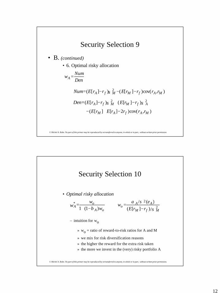
Security Selection 9
• B. (continued)• 6. Optimal risky allocation
σσ 22 )][()][( AfMMfA rrErrEDen −+−=
DenNum
wA =
),cov()][()][( 2MAfMMfA rrrrErrENum −−−= σ
),cov()2][][( MAfAM rrrrErE −+−
© Michel A. Robe. No part of this primer may be reproduced by or transferred to anyone, in whole or in part, without written prior permission.
Security Selection 10
• Optimal risky allocation
– intuition for wo
» wo = ratio of reward-to-risk ratios for A and M
» we mix for risk diversification reasons» the higher the reward for the extra risk taken» the more we invest in the (very) risky portfolio A
σσα
/ 2
2
)][()(/
MfM
AAo rrE
ew
−=
oA
oA w
ww
)1(1*
β−+=

13
© Michel A. Robe. No part of this primer may be reproduced by or transferred to anyone, in whole or in part, without written prior permission.
Security Selection 11
• Optimal risky allocation
– intuition for w*
» w* = adjustment for beta
» the weight for A depends on diversif. opportunities
» if then more can be gained by diversifying
wAMw *1−=oA
oA w
ww
)1(1*
β−+=
1<Aβ
oA ww <⇒ *
© Michel A. Robe. No part of this primer may be reproduced by or transferred to anyone, in whole or in part, without written prior permission.
Security Selection 12• 7. Optimal security weights:
– intuition
» to “max” the composite portfolio’s Sharpe ratio
» given the Sharpe ratio of the market (M) is fixed
» we must maximize the “appraisal” ratio of A:
∑=
= n
jjj
kkk
e
ew
12
2
)(/
)(/
σα
σα
22
2
222
)(][
)(
+
−=+=
A
A
M
fM
A
AMP e
rrEe
SSσσ
ασ
α
)( A
Aeσ
α

14
© Michel A. Robe. No part of this primer may be reproduced by or transferred to anyone, in whole or in part, without written prior permission.
Security Selection 13
• Optimal security weights» given
» and
» we must have:
∑=
= n
jjj
kkk
e
ew
12
2
)(/
)(/
σα
σα
∑=
=n
kkkA w
1αα
∑=
+=n
kkkMAA ew
1
22222 )(σσβσ
© Michel A. Robe. No part of this primer may be reproduced by or transferred to anyone, in whole or in part, without written prior permission.
Security Selection 14
• B. (continued)• 8. Individual security contributions
» the appraisal ratio of each security
» measure its contribution
» to the performance of the active portfolio
∑=
=
n
k k
k
A
Aee 1
22
)()( σσαα

15
© Michel A. Robe. No part of this primer may be reproduced by or transferred to anyone, in whole or in part, without written prior permission.
Security Selection 15
• C. Numerical example• data (BKM6 pp. 992-995 and interpretation)
• Sharpe ratio
%20%;7%;15][ === MfM rrE σ
2/1
1
22
2
22
)(
][
)(
+
−=+= ∑
=
n
k k
k
M
fM
A
AMP e
rrE
eSS
σσα
σα
SS MP2
2/1222 16.
208222.0
%20%8
1154.1563.1556. ==>=
+++=
© Michel A. Robe. No part of this primer may be reproduced by or transferred to anyone, in whole or in part, without written prior permission.
Security Selection 16
• optimal weights (see table)• portfolio characteristics
» large alpha, but large idiosyncratic risk
%56.2003.04735.1)05.0()6212.1(07.01477.1 =+−−+= xxx
∑=
=n
kkkA w
1αα
9519.01
== ∑=
n
kkkA w ββ
%62.82)( =Aeσ 6828.0)(2 =Aeσ

16
© Michel A. Robe. No part of this primer may be reproduced by or transferred to anyone, in whole or in part, without written prior permission.
Security Selection 17
• optimal risky portfolio– despite high alpha, small proportion in active portfolio
» large risk needs to be balanced out
– small adjustment for beta
» beta is close to 1
%95.141495.0)1(1
* ==−+
=oA
oA w
ww
β
1506.0)][(
)(/
/ 2
2=
−=
σσα
MfM
AAo rrE
ew
%05.851 * =−= wAMw
© Michel A. Robe. No part of this primer may be reproduced by or transferred to anyone, in whole or in part, without written prior permission.
Security Selection 18
• performance gain– Sharpe ratio
– M2 measure = 1.42% (large number, given only 3 securities)
» match risk (i.e., std-dev) of portfolio M
» by mixing optimal risky portfolio and T-bills
» in proportions and respectively
SS MP ==>== 4.0%20
%84711.02219.0
σσ
2
2
M
P
σσ
2
21
M
P−
17
© Michel A. Robe. No part of this primer may be reproduced by or transferred to anyone, in whole or in part, without written prior permission.
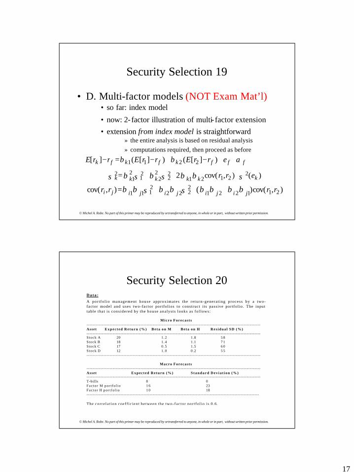
Security Selection 19
• D. Multi-factor models (NOT Exam Mat’l)• so far: index model
• now: 2-factor illustration of multi- factor extension• extension from index model is straightforward
» the entire analysis is based on residual analysis» computations required, then proceed as before
fffkfkfk errErrErrE αββ ++−+−=− )][()][(][ 2211
)(),cov(2 22121
22
22
21
21
2kkkkkk err σββσβσβσ +++=
),cov()),cov( 2112212222
2111 ( rrrr jijijijiji ββββσββσββ +++=
© Michel A. Robe. No part of this primer may be reproduced by or transferred to anyone, in whole or in part, without written prior permission.
Security Selection 20D a t a :
A por t fo l io management house approximates the re turn-genera t ing process by a two-factor model and uses two-factor portfol ios to construct i ts passive portfol io . The inputtable tha t i s considered by the house analys ts looks as fo l lows:
M i c r o F o r e c a s t s-----------------------------------------------------------------------------------------------------------------Asset E x p e c t e d R e t u r n ( % ) B e t a o n M B e t a o n H R e s i d u a l S D ( % )-----------------------------------------------------------------------------------------------------------------Stock A 20 1 .2 1.8 5 8Stock B 18 1 .4 1.1 7 1Stock C 17 0 .5 1.5 6 0Stock D 12 1 .0 0.2 5 5-----------------------------------------------------------------------------------------------------------------
Macro Forecas t s-----------------------------------------------------------------------------------------------------------------Asset E x p e c t e d R e t u r n ( % ) S t a n d a r d D e v i a t i o n ( % )-----------------------------------------------------------------------------------------------------------------T-bills 8 0Fac tor M por t fo l io 1 6 23Fac tor H por t fo l io 1 0 18----------------------------------------------------------------------------------------------------------------
The corre la t ion coeff ic ient be tween the two-fac tor por t fo l io i s 0 .6 .
18
© Michel A. Robe. No part of this primer may be reproduced by or transferred to anyone, in whole or in part, without written prior permission.
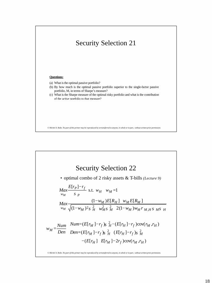
Security Selection 21
Questions:
(a) What is the optimal passive portfolio?(b) By how much is the optimal passive portfolio superior to the single-factor passive
portfolio, M, in terms of Sharpe’s measure?(c) What is the Sharpe measure of the optimal risky portfolio and what is the contribution
of the active portfolio to that measure?
© Michel A. Robe. No part of this primer may be reproduced by or transferred to anyone, in whole or in part, without written prior permission.
Security Selection 22• optimal combo of 2 risky assets & T-bills (Lecture 9)
1 s.t. ][
=+−
MHP
fP
www
rrEMax
M σ
σσσσ ρ HMHMMMMMHM
MMHM
w www
REwREwMax
wM ,2222 )1(2)1(
][][)1(
−++−
+−
DenNum
wM =),cov()][()][( 2
HMfHHfM rrrrErrENum −−−= σ
σσ 22 )][()][( MfHHfM rrErrEDen −+−=
),cov()2][][( HMfMH rrrrErE −+−

19
© Michel A. Robe. No part of this primer may be reproduced by or transferred to anyone, in whole or in part, without written prior permission.
Security Selection 23
σσ 22 )][()][( MfHHfM rrErrEDen −+−=
DenNum
wM =
),cov()][()][( 2HMfHHfM rrrrErrENum −−−= σ
),cov()2][][( HMfMH rrrrErE −+−
© Michel A. Robe. No part of this primer may be reproduced by or transferred to anyone, in whole or in part, without written prior permission.
Security Selection 24
Answers:
(a) The optimal passive portfolio is obtained from equation (7.8) in Chapter 7 on OptimalRisky Portfolios – see Lecture 9.
wM = [E(RM)σH2 – E(RH)Cov(rH, rM)/{E(R M)σH
2 + E(RM)σM2 – [E(R H)+E(RM)]Cov(rH, rM)}
where RM = 8%, RH = 2% and Cov(rH, rM) = ρσMσH = 0.6 x 23 x 18 = 248.4.
Thus, wM = 8 x 182 – (2 x 248.4)/[8 x 18
2 + (2 x 23
2) – (8 + 2) 248.4] = 1.797,
and wH = -0.797.
Because the weight on H is negative, if short sales are not allowed, portfolio H wouldhave to be left out of the passive portfolio.

20
© Michel A. Robe. No part of this primer may be reproduced by or transferred to anyone, in whole or in part, without written prior permission.
Security Selection 25
Answers:
(b)With short sales allowed,
E(Rpassive) = 1.797 x 8 + (-0.797) x 2 = 12.78%
σ2passive = (1.797 x 23)2 + [(-0.797) x 18]2 + 2 x 1.797 x (-0.797) x 248.4 = 1202.54
σpassive = 34.68%.
Sharpe’s measure in this case is given by:
Spassive = 12.78/34.68 = 0.3685,
and compared with the (simple) market’s Sharpe measure of
SM = 8/23 = 0.3478.
© Michel A. Robe. No part of this primer may be reproduced by or transferred to anyone, in whole or in part, without written prior permission.
Security Selection 26
• We now must• research or estimate
• find the active portfolio» −> done (i.e., keep security in passive portf.)
» −> go long
» −> go short
» optimal weights:
kkfMkfk errrr αβ ++−+= )(
0=kα0>kα
0<kα
∑=
= n
jjj
kkk
e
ew
12
2
)(/
)(/
σα
σα1
1=∑
=
n
kkw
21
© Michel A. Robe. No part of this primer may be reproduced by or transferred to anyone, in whole or in part, without written prior permission.
Security Selection 27
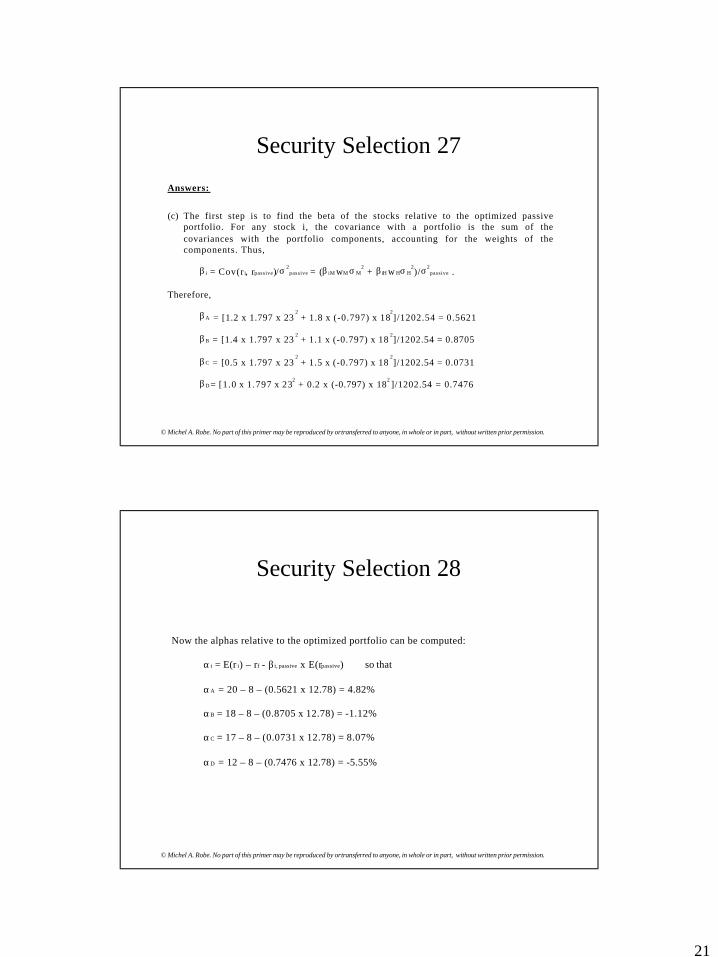
Answers:
(c) The first step is to find the beta of the stocks relative to the optimized passiveportfolio. For any stock i, the covariance with a portfolio is the sum of thecovariances with the portfolio components, accounting for the weights of thecomponents. Thus,
β i = Cov(r i, rpassive)/σ2
passive = (β iM wM σ M2 + β iH w Hσ H
2)/σ
2passive .
Therefore,
βA = [1.2 x 1.797 x 232 + 1.8 x (-0.797) x 18
2]/1202.54 = 0.5621
βB = [1.4 x 1.797 x 232 + 1.1 x (-0.797) x 18
2]/1202.54 = 0.8705
βC = [0.5 x 1.797 x 232 + 1.5 x (-0.797) x 18
2]/1202.54 = 0.0731
βD = [1.0 x 1.797 x 232 + 0.2 x (-0.797) x 18
2]/1202.54 = 0.7476
© Michel A. Robe. No part of this primer may be reproduced by or transferred to anyone, in whole or in part, without written prior permission.
Security Selection 28
Now the alphas relative to the optimized portfolio can be computed:
α i = E(r i) – rf - βi, passive x E(rpassive) so that
αA = 20 – 8 – (0.5621 x 12.78) = 4.82%
αB = 18 – 8 – (0.8705 x 12.78) = -1.12%
αC = 17 – 8 – (0.0731 x 12.78) = 8.07%
αD = 12 – 8 – (0.7476 x 12.78) = -5.55%
22
© Michel A. Robe. No part of this primer may be reproduced by or transferred to anyone, in whole or in part, without written prior permission.
Security Selection 29
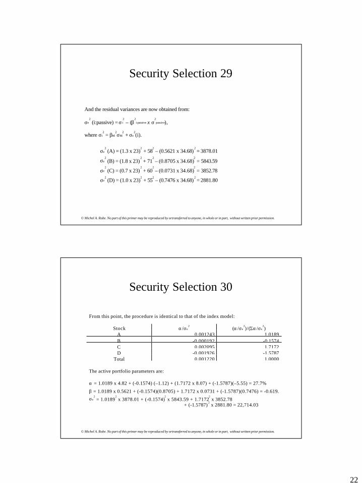
And the residual variances are now obtained from:
σe2 (i:passive) = σ i
2 – (β
2i:passive x σ
2passive),
where σi2 = βM
2σM
2 + σe
2(i).
σe2 (A) = (1.3 x 23)
2 + 58
2 – (0.5621 x 34.68)
2 = 3878.01
σe2 (B) = (1.8 x 23)
2 + 71
2 – (0.8705 x 34.68)
2 = 5843.59
σe2 (C) = (0.7 x 23)
2 + 60
2 – (0.0731 x 34.68)
2 = 3852.78
σe2 (D) = (1.0 x 23)
2 + 55
2 – (0.7476 x 34.68)
2 = 2881.80
© Michel A. Robe. No part of this primer may be reproduced by or transferred to anyone, in whole or in part, without written prior permission.
Security Selection 30
From this point, the procedure is identical to that of the index model:
Stock α/σe2
(α/σe2)/(Σα/σe
2)
A 0.001243 1.0189B -0.000192 -0.1574C 0.002095 1.7172D -0.001926 -1.5787
Total 0.001220 1.0000
The active portfolio parameters are:
α = 1.0189 x 4.82 + (-0.1574) (–1.12) + (1.7172 x 8.07) + (-1.5787)(–5.55) = 27.7%
β = 1.0189 x 0.5621 + (-0.1574)(0.8705) + 1.7172 x 0.0731 + (-1.5787)(0.7476) = -0.619.
σe2 = 1.0189
2 x 3878.01 + (-0.1574)
2 x 5843.59 + 1.7172
2 x 3852.78
+ (-1.5787)2 x 2881.80 = 22,714.03

23
© Michel A. Robe. No part of this primer may be reproduced by or transferred to anyone, in whole or in part, without written prior permission.
Security Selection 31
• Optimal risky allocation (index model)
– intuition for wo
» wo = ratio of reward-to-risk ratios for A and P
» we mix for risk diversification reasons» the higher the reward for the extra risk taken» the more we invest in the (very) risky portfolio A
σσα
/ 2
2
)][()(/
MfM
AAo rrE
ew
−=
oA
oA w
ww
)1(1*
β−+=
© Michel A. Robe. No part of this primer may be reproduced by or transferred to anyone, in whole or in part, without written prior permission.
Security Selection 31
The proportions in the overall risky portfolio can now be determined:
w0 = (α/σe2)/[E(Rpassive)/σ2
passive] = (27.71/22,714.03)/(12.78/1202.54) = 0.1148.
w* = 0.1148/[1 + (1 + 0.6190) x 0.1148] = 0.0968.
Sharpe’s measure for the optimal risky portfolio is:
S2 = S2passive + (α/σe)2 = 0.36852 + [27.712/22,714.03] = 0.1696
S = 0.4118,
compared to Spassive = 0.3685.

24
© Michel A. Robe. No part of this primer may be reproduced by or transferred to anyone, in whole or in part, without written prior permission.
Security Selection 32
• E. Potential benefits (Treynor-Black)• in practice
– not yet used often widely» hard to estimate alphas (bias correction needed)» correction requires constant monitoring & appraisal» shows alphas imprecise, second-guesses analysts
» do you think analysts like that?
• yet, significant benefits» easy to implement» allows for decentralized decisions» can add significant return» amenable to multi-factor analysis
© Michel A. Robe. No part of this primer may be reproduced by or transferred to anyone, in whole or in part, without written prior permission.
Part VI.B:Active Portfolio
Management Evaluation

25
© Michel A. Robe. No part of this primer may be reproduced by or transferred to anyone, in whole or in part, without written prior permission.
Portfolio Performance Evaluation
• Returns• return measurement over several periods
• Performance measures • market timing• security analysis
» Treynor, Sharpe, Jensen, appraisal ratio, M2
» practical cases
• Performance attribution• bogey; asset allocation; sector and security decisions
© Michel A. Robe. No part of this primer may be reproduced by or transferred to anyone, in whole or in part, without written prior permission.
Portfolio Return Measurement
• One period vs. multiple periods• easy vs. unclear
» depends on number of periods» affected by intermediate investments/withdrawals
• Time-weighted vs. dollar-weighted• average return vs. IRR• examples (Table 24.1)• why use a time average?
» performance measurement assigns responsibilities» cash ins and outs?
26
© Michel A. Robe. No part of this primer may be reproduced by or transferred to anyone, in whole or in part, without written prior permission.
Portfolio Return Measurement 2
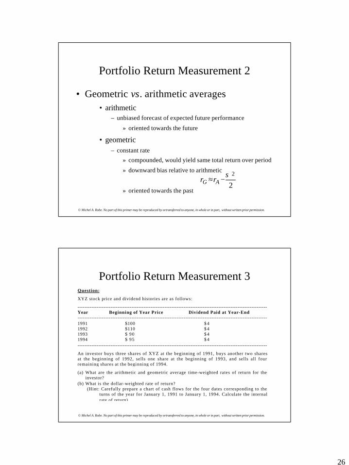
• Geometric vs. arithmetic averages• arithmetic
– unbiased forecast of expected future performance
» oriented towards the future
• geometric– constant rate
» compounded, would yield same total return over period
» downward bias relative to arithmetic
» oriented towards the past2
2σ−≈ AG rr
© Michel A. Robe. No part of this primer may be reproduced by or transferred to anyone, in whole or in part, without written prior permission.
Portfolio Return Measurement 3Question:
XYZ stock price and dividend histories are as follows:
-------------------------------------------------------------------------------------------------------------Year Beginning of Year Price Dividend Paid at Year-End-------------------------------------------------------------------------------------------------------------1991 $100 $ 41992 $110 $ 41993 $ 90 $ 41994 $ 95 $ 4-------------------------------------------------------------------------------------------------------------
An investor buys three shares of XYZ at the beginning of 1991, buys another two sharesat the beginning of 1992, sells one share at the beginning of 1993, and sells all fourremaining shares at the beginning of 1994.
(a) What are the arithmetic and geometric average time-weighted rates of return for theinvestor?
(b) What is the dollar-weighted rate of return? (Hint: Carefully prepare a chart of cash flows for the four dates corresponding to the
turns of the year for January 1, 1991 to January 1, 1994. Calculate the internalrate of return).

27
© Michel A. Robe. No part of this primer may be reproduced by or transferred to anyone, in whole or in part, without written prior permission.
Portfolio Return Measurement 4
Answer:
(a) Time-weighted average returns are based on year-by-year rates of return.
Year Return [(capital gains + dividend)/price)]------------------------------------------------------------------------------1991-1992 [(110-100) + 4]/100 = 14%1992-1993 [(90 – 110) + 4]/110 = -14.55%1993-1994 [(95 – 90) + 4 ]/90 = 10%------------------------------------------------------------------------------
Arithmetic mean = 3.15%Geometric mean = 2.33%
© Michel A. Robe. No part of this primer may be reproduced by or transferred to anyone, in whole or in part, without written prior permission.
Portfolio Return Measurement 5
(b)
Time Cash Flow Explanation-------------------------------------------------------------------------------------------------------------0 -300 Purchase of 3 shares at $100 each.1 -208 Purchase of 2 shares at $110 less dividend income on 3 share s held2 110 Dividends on 5 shares plus sale of one share at price of $90 each.3 396 Dividends on 4 shares plus sale of 4 shares at price of $95 each.-------------------------------------------------------------------------------------------------------------
$110 $396______________________________________|____________|_____Date 1/1/91 1/1/92 1/1/93 1/1/94
| |($300) ($208)
Dollar-weighted return = Internal rate of return of cash-flow series = -0.1661%.

28
© Michel A. Robe. No part of this primer may be reproduced by or transferred to anyone, in whole or in part, without written prior permission.
Market Timing Evaluation
• Idea• market timers shift money (MM <−> risky portfolio)
» based on their forecasts of market return
• return from market timing » depends on # of times the timer is correct
• two scenarios: bull vs. bear– must be correct in each scenario
» example 1: always predict snow in Winter in Montrealright 95% of the timebut always wrong when no snow
» example 2: forward hedges
• overall quality vs. risk adjustment
© Michel A. Robe. No part of this primer may be reproduced by or transferred to anyone, in whole or in part, without written prior permission.
Market Timing Evaluation 2
• Overall quality• measure 1
– measure = P1 + P2 - 1
» P1 = proportion of correct bull predictions
= 1 if 100% correct
» P2 = proportion of correct bull predictions
= 1 if 100% correct
– example: return maximization
» correct 100% of bulls, 0% of bears −> measure = 0
» correct 50% of bulls, 50% of bears -> measure = 0

29
© Michel A. Robe. No part of this primer may be reproduced by or transferred to anyone, in whole or in part, without written prior permission.
Market Timing Evaluation 3
• Overall quality• measure 2
– unclear
» how large (P1 + P2 - 1) must be
» to ensure that we have seen “good performance”
– solution
» statistical significance» application: hedging decisions (as time allows)
© Michel A. Robe. No part of this primer may be reproduced by or transferred to anyone, in whole or in part, without written prior permission.
Market Timing Evaluation 4
• Risk adjustment• problems
» neither measure so far accounts for risk» market timers constantly change portfolio risk profile
• solutions
» time-varying dummy D (=1 for bull, 0 for bear)
» Squared term
PfMfMfP eDrrcrrbarr +−+−+=− )()(
PfMfMfP eDrrcrrbarr +−+−+=− )()(
30
© Michel A. Robe. No part of this primer may be reproduced by or transferred to anyone, in whole or in part, without written prior permission.
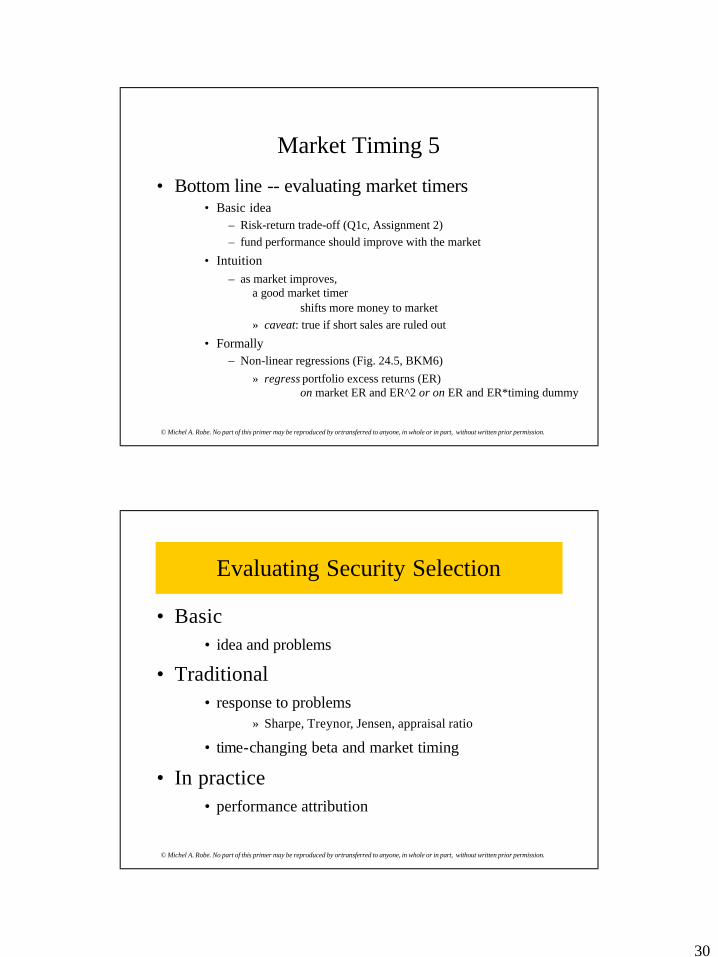
Market Timing 5
• Bottom line -- evaluating market timers• Basic idea
– Risk-return trade-off (Q1c, Assignment 2)– fund performance should improve with the market
• Intuition– as market improves,
a good market timer shifts more money to market
» caveat: true if short sales are ruled out
• Formally– Non-linear regressions (Fig. 24.5, BKM6)
» regress portfolio excess returns (ER) on market ER and ER^2 or on ER and ER*timing dummy
© Michel A. Robe. No part of this primer may be reproduced by or transferred to anyone, in whole or in part, without written prior permission.
Evaluating Security Selection
• Basic• idea and problems
• Traditional• response to problems
» Sharpe, Treynor, Jensen, appraisal ratio
• time-changing beta and market timing
• In practice• performance attribution

31
© Michel A. Robe. No part of this primer may be reproduced by or transferred to anyone, in whole or in part, without written prior permission.
Evaluating Security Selection 2
• Basic• idea
– compare returns with those of “similar” portfolios
– depict percentiles (BKM 4-5-6, Fig. 24.1)
» ex.: manager outperforms 90 out of 100 fund managersis in the 90th percentile
» 5th, 95th percentiles; median, 25th and 75th_
• problems– equities: allocations differ within groups
– fixed income: durations vary
© Michel A. Robe. No part of this primer may be reproduced by or transferred to anyone, in whole or in part, without written prior permission.
Evaluating Security Selection 3
• Traditional• idea
– account for risk taken by manager
– assume index model holds (and past performance matters)
» and compute risk-adjusted excess returns
• problems– does extra performance cover fees
» difficulty to beat S&P 500
– estimation in practice
» statistical significance?
32
© Michel A. Robe. No part of this primer may be reproduced by or transferred to anyone, in whole or in part, without written prior permission.
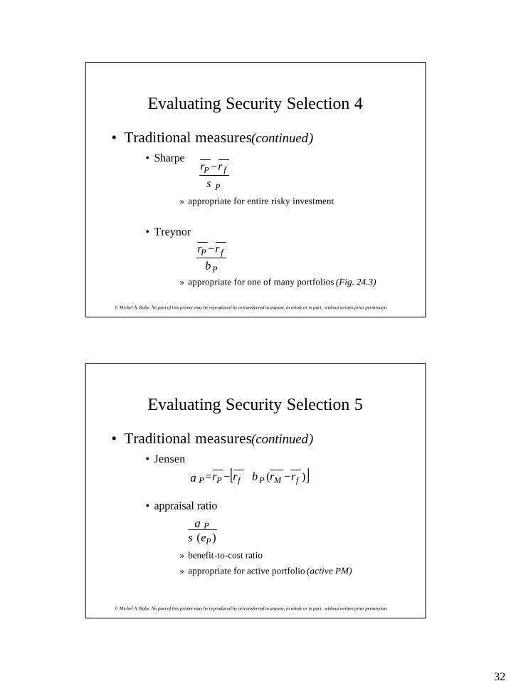
Evaluating Security Selection 4
• Traditional measures(continued)• Sharpe
» appropriate for entire risky investment
• Treynor
» appropriate for one of many portfolios (Fig. 24.3)
P
fP rrσ−
P
fP rrβ−
© Michel A. Robe. No part of this primer may be reproduced by or transferred to anyone, in whole or in part, without written prior permission.
Evaluating Security Selection 5
• Traditional measures(continued)• Jensen
• appraisal ratio
» benefit-to-cost ratio
» appropriate for active portfolio (active PM)
)( P
Peσ
α
[ ])( fMPfPP rrrr −+−= βα
33
© Michel A. Robe. No part of this primer may be reproduced by or transferred to anyone, in whole or in part, without written prior permission.
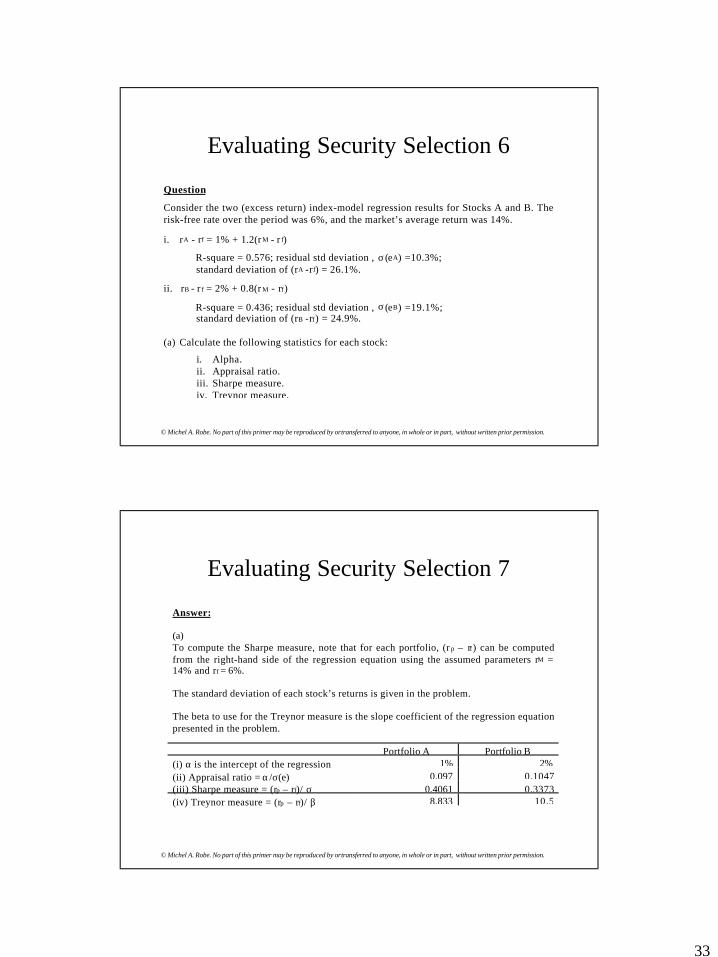
Evaluating Security Selection 6
Question
Consider the two (excess return) index-model regression results for Stocks A and B. Therisk-free rate over the period was 6%, and the market’s average return was 14%.
i. rA - rf = 1% + 1.2(r M - r f)
R-square = 0.576; residual std deviation , σ(eA) =10.3%; standard deviation of (rA -rf) = 26.1%.
ii. rB - r f = 2% + 0.8(r M - rf)
R-square = 0.436; residual std deviation , σ(eB) =19.1%; standard deviation of (rB -rf) = 24.9%.
(a) Calculate the following statistics for each stock:
i. Alpha.ii. Appraisal ratio.iii. Sharpe measure.iv. Treynor measure.
© Michel A. Robe. No part of this primer may be reproduced by or transferred to anyone, in whole or in part, without written prior permission.
Evaluating Security Selection 7
Answer:
(a)To compute the Sharpe measure, note that for each portfolio, (r p – rf) can be computedfrom the right-hand side of the regression equation using the assumed parameters rM =14% and rf = 6%.
The standard deviation of each stock’s returns is given in the problem.
The beta to use for the Treynor measure is the slope coefficient of the regression equationpresented in the problem.
Portfolio A Portfolio B(i) α is the intercept of the regression 1% 2%(ii) Appraisal ratio = α/σ(e) 0.097 0.1047(iii) Sharpe measure = (rp – rf)/ σ 0.4061 0.3373(iv) Treynor measure = (rp – rf)/ β 8.833 10.5

34
© Michel A. Robe. No part of this primer may be reproduced by or transferred to anyone, in whole or in part, without written prior permission.
Evaluating Security Selection 8
(b) Which stock is the best choice under the following circumstances?
i. This is the only risky asset to be held by the investor.ii. This stock will be mixed with the rest of the investor’s portfolio, currently
composed solely of holdings in the market index fund.iii. This is one of many stocks that the investor is analyzing to form an actively
managed stock portfolio.
© Michel A. Robe. No part of this primer may be reproduced by or transferred to anyone, in whole or in part, without written prior permission.
Evaluating Security Selection 9
Answer:
(a) (i) If this is the only risky asset, then Sharpe’s measure is the one to use.A’s is higher, so it is preferred.
(ii) If the portfolio is mixed with the index fund, the contribution to the overall Sharpemeasure is determined by the appraisal ratio.Therefore, B is preferred.
(iii) If it is one of many portfolios, then Treynor’s measure counts, and B is preferred.

35
© Michel A. Robe. No part of this primer may be reproduced by or transferred to anyone, in whole or in part, without written prior permission.
Evaluating Security Selection 10
• Problems• does extra performance cover fees?
» difficulty to beat S&P 500
• estimation in practice?» statistical significance?
» time-varying beta? (Fig. 24.4)
» solution: add a quadratic term in regression (Fig. 24.5)
• bottom line» still used
» but not so much any more
© Michel A. Robe. No part of this primer may be reproduced by or transferred to anyone, in whole or in part, without written prior permission.
Performance Attribution
• Idea• hard to evaluate managers on risk-adjusted basis• important to allocate bonuses
• Split• excess returns
• between contributions» broad asset allocation
» industry choices within each market
» security choices within each sector

36
© Michel A. Robe. No part of this primer may be reproduced by or transferred to anyone, in whole or in part, without written prior permission.
Performance Attribution 2
• Bogey (BKM6 Table 24.5)
• base-line passive portfolio• assumed fixed for investment horizon
• Splits (BKM6 Tables 24.6 to 24.8)
• broad asset» compare to bogey
• industry» given weights, compare with market weights
• security
© Michel A. Robe. No part of this primer may be reproduced by or transferred to anyone, in whole or in part, without written prior permission.
Performance Attribution 3Question 9 (20 points)
Consider the following information regarding the performance of a money manager in arecent month. The table represents the actual return of each sector of the manager’sportfolio in Column 1, the fraction of the portfolio allocated to each sector in Column 2,the benchmark or neutral sector allocations in Column 3, and the returns of sector indicesin Column 4.
Actual Return Actual Weight Benchmark Weight Index Return-----------------------------------------------------------------------------------------------------------------Equity 2% 0.70 0.60 2.5% (S&P 500)Bonds 1% 0.20 0.30 1.2% (SB Index)*Cash 0.5% 0.10 0.10 0.5%-----------------------------------------------------------------------------------------------------------------* S&B Index = Salomon Brothers Index.
(a) What was the manager’s return in the month? What was his or her overperformanceor underperformance?
(b) What was the contribution of security selection to relative performance?(c) What was the contribution of asset allocation to relative performance? Confirm that
the sum of selection and allocation contributions equals his or her total “excess”return relative to the bogey.

37
© Michel A. Robe. No part of this primer may be reproduced by or transferred to anyone, in whole or in part, without written prior permission.
Performance Attribution 4Answer:
(a) Bogey: 0.60 x 2.5% + 0.30 x 1.2% + 0.10 x 0.5% = 1.91% Actual: 0.70 x 2.0% + 0.20 x 1.0% + 0.10 x 0.5% = 1.65% Underperformance: 0.26%
(a) Security Selection:
Market Differential Return Manager’s Portfolio Contributio nWithin Market Weight to
Performance-------------------------------------------------------------------------------------------------------------Equity -0.5% 0.70 -0.35%Bonds -0.2% 0.20 -0.04%Cash 0 0.10 0%-------------------------------------------------------------------------------------------------------------Contribution of security selection -0.39%------------------------------------------------------------------------------------------------------------------------------------
© Michel A. Robe. No part of this primer may be reproduced by or transferred to anyone, in whole or in part, without written prior permission.
Performance Attribution 5(a) Asset Allocation:
Market Excess Weight: Index Return ContributionManager - Benchmark minus Bogey to
Performance---------------------------------------------------------------------------------------------------------------------Equity 0.1 0 0.59% 0 .059%Bonds -0.10 -0.71% 0 .071%Cash 0 -1.41% 0 %---------------------------------------------------------------------------------------------------------------------Contribution of asset allocation 0.13%---------------------------------------------------------------------------------------------------------------------
Summary: Security selection = -0.39%Asset allocation = 0.13% Excess performance = -0.26%