Partial Fiscal Decentralization and Demand Responsiveness of theLocal Public Sector: Theory and Evidence from Norway

by

Lars-Erik Borge

Department of Economics

Norwegian University of Science and Technology

N-7491 Trondheim, Norway

Jan K. Brueckner

Department of Economics

University of California, Irvine

Irvine, CA 92697 USA

Jorn Rattsø

Department of Economics

Norwegian University of Science and Technology

N-7491 Trondheim, Norway

March 2012, latest revision September 2013

Abstract

This paper provides an empirical test of a principal tenet of fiscal federalism: that spending

discretion, when granted to localities, allows public-good levels to adjust to suit local demands.

The test is based on a simple model of partial fiscal decentralization, under which earmarking

of central transfers for particular uses is eliminated, allowing funds to be spent according to

local tastes. The greater role of local demand determinants following partial decentralization

is confirmed by the paper’s empirical results, which show the effects of the 1986 Norwegian

reform.

Partial Fiscal Decentralization and Demand Responsiveness of theLocal Public-Sector: Theory and Evidence from Norway

by

Lars-Erik Borge, Jan K. Brueckner, and Jorn Rattsø∗

1. Introduction

With fiscal decentralization, subnational governments gain autonomy in the provision and

financing of public goods. Such autonomy has been a longtime feature of fiscal arrangements in

the United States, Canada and a few other countries. A greater degree of central management

of the public sector, however, is common elsewhere, especially in developing countries. But

partly in response to advice from the World Bank and other international agencies, many

countries are embracing fiscal decentralization by attempting to devolve spending and taxing

authority to subnational governments. This movement is motivated in part by the lessons of

the Tiebout (1956) model, which show that local control of spending allows the public sector

to better respond to heterogeneous demands for public goods.

Despite these developments, the fiscal decentralization pursued in other parts of the world

often fails to match the North American pattern, being only partial in nature. Rather than

gaining autonomy to set both spending and taxes, subnational governments often must rely

on transfers from the central government to finance the provision of public goods.1 With

fixed transfers, subnational governments often have little latitude in choosing the levels of

public goods, especially when transfers are accompanied by mandates that specify how the

money is to be allocated across spending categories. This reliance on transfers, and the lack

of discretion it entails, is often a result of a lack of tax capacity at the subnational level. For

either historical or constitutional reasons, subnational governments may not have access to

taxes capable of generating substantial revenue, in contrast to the situation in North America,

where subnational income, sales and property taxes generate enormous revenue. Alternatively,

productive subnational taxes may exist but their rates may be centrally controlled.2

Despite its relevance in much of the world, partial fiscal decentralization has received only

1

limited treatment in the public economics literature. One purpose of the present paper is to

offer a simple new model that compares public-good provision under partial decentralization

to the outcomes under centralized provision and, alternatively, “full” decentralization, where

subnational governments gain complete fiscal autonomy. The model yields clearcut predictions

showing how a movement from centralization to partial decentralization affects public-good

provision, and these predictions are then tested using data from Norway. A 1986 Norwegian

reform gave local governments more control over spending decisions while maintaining their

reliance on central transfers as a source of funds, and the empirical work investigates the effect

of this reform.

The model builds on the analysis of Brueckner (2009), which also compared outcomes un-

der centralization, partial, and full decentralization. In a model like Brueckner’s that has only

a single public good (denoted z), a local government relying on a fixed central transfer under

partial decentralization would ordinarily have no discretion in its choices, with the z level au-

tomatically determined by the transfer amount. However, public-good levels in Brueckner’s

model are determined both by spending and by the “effort” level of local governments, breaking

the direct link between the transfer and z.3 The present model differs fundamentally by as-

suming provision of two distinct public goods (x and z) rather than one, with local-government

effort dropped as an input. Local discretion under partial decentralization now exists despite

the fixed transfer because local governments are free to choose the mix of the two public goods,

varying the levels of x and z to suit local preferences while holding total spending constant

at the amount of the transfer. The simple prediction of the model is that, with per capita

spending held fixed, moving from centralization (where the center sets uniform levels of the

two public goods) to partial decentralization leads to heterogeneity in the levels of the goods.

Under partial decentralization, the x and z levels in different localties diverge from the common

level under centralization, reflecting local demand differences, even though total spending is

held constant.

The model thus predicts that, following partial decentralization, local characteristics af-

fecting the demand for public goods play a greater role in determining provision levels than

before. Evidence for this enhanced role comes from studying the effects of the 1986 Norwegian

2

reform, which relaxed the spending mandates for individual public goods that were part of

the previous system of intergovernmental grants. This change allowed new local discretion in

the choice of the public-good mix while keeping the size of grants constant, representing the

kind of partial decentralization envisioned in the model. In effect, the 1986 reform offers a

natural experiment that allows a rare test of the effects of local discretion. Pre- and post-

reform demand estimates show that local characteristics gained explanatory power following

the reform, indicating that the reform allowed public-good provision to adjust in response to

demand heterogeneity across jurisdictions. By allowing greater local discretion, the reform

may have also raised the incentives for the sorting of the population according to preferences

for public goods. The paper offers evidence that intercity migration increased following the

reform, which may reflect greater sorting incentives.

The paper’s demonstration of the enhanced role of local demand determinants following

the reform offers support for a fundamental tenet of fiscal federalism, namely, that local fis-

cal discretion enables the public sector to better respond to consumer preferences for public

goods. Despite this idea’s central importance in the vast literature on the Tiebout hypothesis,

empirical work designed to explicitly test it is scarce. In one study, Ahlin and Mork (2008)

exploit a similar natural experiment in Sweden that allowed greater local discretion in the

determination of school spending, although they find mixed results that lend little support

for the hypothesis. Earlier work by Borge and Rattsø (1993) also explored the effects of the

Norwegian reform, but their approach did not deliver clearcut findings like those presented be-

low. In contrast, Faguet (2004) found that when a Bolivian reform raised central-government

transfers and gave localities more control over investment projects, investment levels changed

in ways that reflected local characteristics.4 With only one prior empirical study establishing

such a conclusion, more evidence is needed, and this paper provides it. Note also that the

current evidence relates to public-service provision, not public investment.

Instead of addressing the role of local demand determinants and exploiting such natural

experiments, most previous work in the Tiebout tradition has investigated the foundational

aspects of the theory. Oates (1969) and the vast ensuing literature on capitalization validates

the premise that public goods matter to consumers and that interjurisdictional mobility regis-

3

ters these preferences, with house prices high in places with high public-good levels. Another

foundational notion, that consumers vote with their feet in pursuing ideal levels of public

spending, is tested in various studies. Some papers, including Pack and Pack (1978), Eberts

and Gronberg (1981) and Rhode and Strumpf (2003), carry out tests for convergence toward

a homogeneous community structure (an implication of voting with one’s feet), while Banzhaf

and Walsh (2008) look more explicitly for evidence of such behavior. A related literature ex-

plores intercommunity residence patterns using more-sophisticated econometric methods, with

the goal of inferring the existence of consumer sorting across jurisdictions (see, for example,

Bayer and Timmins (2007)). The present paper complements all of this previous work by

providing a more-direct test of a core idea of fiscal federalism.

The paper also adds to a recent resurgence of theoretical research on fiscal decentralization,

which builds on the classic treatment of Oates (1972) (see also Wildasin (1986)). Recent papers

include Lockwood (2002), Besley and Coate (2003), Brueckner (2004), Lorz and Willman

(2005), and Arzaghi and Henderson (2005), among others. The models of Besley and Coate

and Lockwood offer a contrast to the present approach by assuming that, when it exercises

control, the central government can differentiate the provision of public goods across local

jurisdictions, blurring the distinction between the centralized and decentralized cases.

In addition to Brueckner (2009), recent work that explicitly focuses on partial fiscal decen-

tralization includes an earlier paper by Schwager (1999), who analyzes what he calls “admin-

istrative federalism.”5 Peralta (2012) constructs a related model with imperfect information

and rent-seeking politicians, where partial decentralization allows more scope for this activity

than full decentralization.6 The analysis of Hatfield and Padro i Miguel (2011) reflects a dif-

ferent view of partial decentralization. In their model, which has a continuum of public goods,

partial decentralization emerges when a portion of the continuum is provided locally, with the

remainder provided by the central government.7 In addition to these papers and those cited

above, many more recent studies bear some connection to the present work.8

The plan of the paper is as follows. Section 2 presents the model, and section 3 gives an

overview of the Norwegian reform on which the empirical work is based. Section 4 discusses

the data and presents the regression results on the role of demand determinants. Section 5

4

presents the migration results, and conclusions are offered in section 6.

2. The Model

Consider an economy where individuals consume two public goods, x and z, along with

a private good e. In order to avoid consideration of jurisdiction sizes, each public good is

assumed to be a publicly produced private good with cost per capita equal to 1 (the model’s

main implications would hold more generally). The economy has two consumer types denoted

by i = 1, 2, who have different Cobb-Douglas preferences given by

ui = αilog(e) + βilog(x) + (1 − αi − βi)log(z), i = 1, 2, (1)

and common incomes equal to I . The share of the type-1 consumers in the overall population

equals δ, with the type-2 population share equal to 1 − δ. The economy contains a number

of local jurisdictions (referred to subsequently as “cities”), with decisions on their public-good

levels made by majority voting in situations where local control is allowed. In “type-1” cities,

type-1 consumers are in the majority, with public-good levels chosen to reflect their preferences,

while type-2 cities have type-2 majorities. Although, in an extreme case, cities could be

homogeneous, with the consumer types segregated in separate jurisdictions, the analysis applies

regardless of the degree of intermixing of the types. But cities of both types are assumed to

exist, so that one type of consumer is not in the majority everywhere. This latter outcome

would emerge, for example, if cities were identical, with their common composition reflecting

the overall population shares of the types. Once the analysis is complete, an extension to an

economy with more than two consumer types is discussed.

2.1. Public-good levels under different degrees of decentralization

The goal of the analysis is to compare the levels of the public goods under three regimes:

centralization, partial decentralization and full decentralization. The comparison between

centralization and partial decentralization is the relevant one for the empirical work, but the

other comparisons yield some additional useful conclusions.

In the case of full decentralization, public-good choices are made locally, with spending

financed by head taxes. The chosen levels of the goods in the different city types are given by

5

familiar demand functions associated with Cobb-Douglas preferences. In a type-i city, the z

and x choices are

x∗i = βiI, z∗i = (1 − αi − βi)I, i = 1, 2. (2)

Total per capita spending on the goods (equal to the city head tax T ∗i ) is

x∗i + z∗i = T ∗

i = (1 − αi)I, i = 1, 2. (3)

Note from (3) that a type’s total spending on public goods varies inversely with its strength

of preference for the private good e, as represented by αi.

Suppose, on the other hand, that public-good levels are dictated by the central government,

with the goods still provided locally but at levels that are uniform across cities despite differing

majority preferences. The local expenditure is financed by uniform per capita grants (supported

by nationally uniform head taxes) sufficient to fund the specified public-good levels.

The mandated public-good levels set by the central government are assumed to equal

weighted averages of the x and z levels that would be chosen under full decentralization, with

the type-1 weight equal to θ. Thus,

x∗ = θx∗1 + (1 − θ)x∗

2, z∗ = θz∗1 + (1 − θ)z∗2. (4)

This rule could reflect the choices of a benevolent central government that knows individual

preferences and seeks to maximize total utility in the economy. In this case, θ would equal δ,

the type-1 population share, as can be seen by computing this welfare-maximizing solution.

Alternatively, (5) could be the result of a political process in which θ captures the extent

of political influence of the type-1 consumers in the centralized choice process (θ > δ would

indicate outsize influence).

Given (4), total per capita spending T ∗ on the public goods under centralization (equal to

the uniform grant and head tax) is a weighted average of the T ∗i from (3). It equals

T ∗ = θT ∗1 + (1 − θ)T ∗

2 = x∗ + z∗. (5)

6

Suppose now that the central government switches to partial fiscal decentralization by

providing the cities with equal per capita grants of T ∗ (again financed by uniform head taxes)

without specifying the particular levels of public goods that must be provided. In other words,

the central government allows freedom of choice in selecting public-good levels, subject to the

requirement that total spending is the same as under centralization. Again, the goods must

be entirely paid for with grant funds. Each city faces the following constraints:

e = y − T ∗, x + z = T ∗. (6)

The chosen public-good levels for the two city types are now

zi =1 − αi − βi

1 − αiT ∗ =

(1 −

βi

1 − αi

)T ∗, xi =

βi

1 − αiT ∗, i = 1, 2. (7)

Note that each public-good level equals T ∗ times the relative preference weight for that good

within the set of public goods. This weight equals the good’s preference coefficient in (1)

divided the sum of x and z coefficients, a sum that equals 1 − αi − βi + βi = 1 − αi.

2.2. Moving from centralization to partial decentralization

The following analysis carries out comparisons of public-good levels under the three re-

gimes, moving from centralization to partial decentralization to full decentralization, and this

section focuses on the first of these movements. To compare x values between centralization

and partial decentralization, (2) and (3) can be used to write x∗i = βiT

∗i /(1−αi). Substituting

in (4) and assuming

β1

1 − α1

<β2

1 − α2

(8)

yields

x∗ =β1

1 − α1

θT ∗1 +

β2

1 − α2

(1−θ)T ∗2 >

β1

1 − α1

θT ∗1 +

β1

1 − α1

(1−θ)T ∗2 =

β1

1 − α1

θT ∗ = x1.

(9)

7

If β2/(1 − α2) appears in place of β1/(1 − α1) in the last two expressions in (9), then the

reverse inequality holds, so that x∗ < x2. Since a parallel argument establishes the opposite

relatioship among the zi’s, it follows that

β1

1 − α1

<β2

1 − α2

=⇒ x1 < x∗ < x2, z1 > z∗ > z2, (10)

with the x and z inequalities reversed if β1/(1 − α1) > β2/(1 − α2).

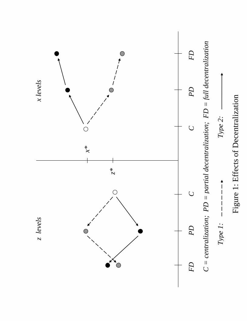
Therefore, in moving from centralization to partial decentralization, the public-good lev-

els diverge from the common centralized level, with x falling (rising) in the city type with

the weaker (stronger) relative preference weight for x. The levels of z move in the opposite

directions. Since total spending on public goods remains fixed at the centralized level T ∗ in

moving to partial decentralization, private-good consumption remains at the centralized level

e∗, with adjustment occurring only in the mix of public goods in response the relative pref-

erence weights for x and z in the two types of cities. In Figure 1, the movement from the C

to PD outcomes illustrates the pattern in (10). Note that x∗ > z∗ is assumed in the figure in

locating the starting point under centralization, and that the FD case is yet to be discussed.

Empirically, (10) and Figure 1 predict that, when partial decentralization occurs, public-

good levels diverge from the common centralized levels in ways that reflect local preferences

for the two goods, leading to different mixes of x and z in across cities. This conclusion clearly

generalizes to a situation with more than two preference types,9 and it forms the basis for the

ensuing empirical work.

2.3. Moving from partial to full decentralization

The movement from partial to full decentralization is more easily analyzed, focusing first

on the case where α1 > α2. First, note that α1 > α2 implies T ∗1

< T ∗2

from (3), so that total

spending on public goods under full decentralization is higher in type-2 cities. Since T ∗ is a

weighted average of the T ∗i from (5), it then follows that T ∗

1< T ∗ < T ∗

2. Next, using (3) to

replace I in (2) with T ∗i /(1 − αi), it follows that x∗

i and z∗i are proportional to T ∗i , with the

same proportionality factors that relate xi and zi to T ∗ in (7). Since the movement from a

common spending level of T ∗ under partial decentralization raises (lowers) total spending on

8

public goods in type-2 (type-1) cities, and since x and z are given by constant proportions of

total spending in both cases, this movement leads to a increase (decrease) in the levels of both

public goods in type-2 (type-1) cities. Thus,

α1 > α2 =⇒ x∗1 < x1, z∗1 < z1; x∗

2 > x2, z∗2 > z2, (12)

with the inequalities reversed when α1 > α2.

The conclusion in (12) follows because total spending on public goods is lower in type-1 than

in type-2 cities under full decentralization (T ∗1

< T ∗2) as a result of their stronger preference for

the private good e, while the x/z mix remains under local control. The conclusion is illustrated

in Figure 1 by the movements from PD to FD. The figure shows that the increase in x2 in

moving from C to PD is amplified by the further movement to FD, and that the decline in x1

is also amplified, widening the gap between the x’s. But the left side of the figure shows that

the gap between z1 and z2 resulting from the C-to-PD movement is narrowed by the further

movement from PD to FD, leaving the z comparison across the city types ambiguous without

further information (the figure is drawn with z∗2

> z∗1).

These conclusions can be seen directly from the solutions, given the assumptions reflected

in the figure. With α1 > α2, satisfaction of β1/(1 − α1) < β2/(1 − α2) requires β1 < β2, so

that x∗1

< x∗2

holds from (2). But the first and third inequalities imply that the comparison

between 1 − α1 − β1 and 1 − α2 − β2, and thus the comparison between z∗1

and z∗2

from (2),

is ambiguous. Therefore, comparison of z∗1 and z∗2 requires an additional explicit assumption

about the relative magnitudes of 1 − αi − βi, i = 1, 2. In general, these findings imply that

the high-α type will have the lower x level under FD if its public-good preferences favor z,

with the z comparison being ambiguous without an additional assumption. If its preferences

instead favor x, the high-α type will have the lower z level under FD, with the x comparison

being ambiguous.

2.4. Empirical framework

The divergence in public-good levels that occurs in moving from centralization to partial

decentralization, as seen in (10) and Figure 1, motivates the ensuing empirical work. However,

9

the empirical context differs from the stylized model in a number of ways, which must be taken

into account. First, cities have different incomes in addition to differences in preferences. In

Norway, however, the effect of income variation is muted by equalization grants, which partly

offset income differences across localities. Second, public goods are financed partly by local

tax revenue in addition to central transfers.

While more detail on these institutional factors is given in section 3 below, it is useful

generalize the previous model somewhat to incorporate them. Let preferences be written more

generally than in the previous framework, with utility given by U(e, x, z; γ), where γ is a vector

of K taste parameters, (γ1, . . . , γK). Let a city again be identified according to the type of

its majority voter, with a type-i city having γ = γi and, recognizing that incomes differ, an

income level of Ii. Ignoring for the moment the presence of local tax revenue, the utility of the

majority voter in a type-i city is U(Ii − T ∗, xi, T ∗ − xi; γi). Under centralization, xi = x∗

and zi = z∗, and since these centrally chosen public-good levels do not vary across cities,

∂xi

∂γik

= 0, k = 1, . . . , K;∂xi

∂Ii= 0, (13)

with the same equalities holding for zi.

While public-good levels are thus unresponsive to the city characteristics (those of its ma-

jority voter) under centralization, they are chosen under partial decentralization to maximize

the previous utility expression in a type-i city, leading to xi = xi. The first-order condition

is Ωi ≡ U ix − U i

z = 0 or U ix/U i

z = 1, where the subscripts denote partial derivatives and the i

subscript indicates that the marginal utilities are evaluated at type-i values.

The second-order condition is Ωix < 0, and differentiating the first-order condition, the

effects of the preference parameters and income on xi are given by

∂xi

∂γik

= −Ωi

γik

Ωix

' U izγik

− U ixγik

, k = 1, . . . , K (14)

∂xi

∂Ii= −

Ωie

Ωix

' U ize − U i

xe, (15)

10

where ' means “has same sign as.” Analogous equations give impacts on zi. Therefore, under

partial decentralization, city characteristics affect public-good levels, as seen in the previous

analysis. Eq. (14) shows that the impact of the taste parameter γik on xi depends on the

difference between its effects on the marginal utilities of z and x, capturing the taste effects

seen in the earlier analysis. While income differences were previously suppressed, (15) shows

that the effect of a higher income on xi depends on the difference between the effects of private

consumption e on the marginal utilities of z and x. Note that since total public spending is

fixed at the central-transfer amount T ∗, the usual income effect that shifts this total is absent.

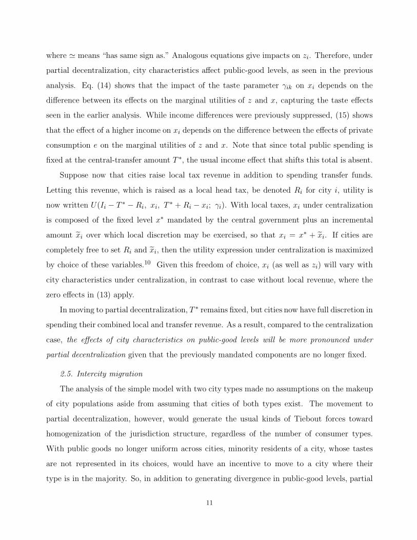
Suppose now that cities raise local tax revenue in addition to spending transfer funds.

Letting this revenue, which is raised as a local head tax, be denoted Ri for city i, utility is

now written U(Ii − T ∗ − Ri, xi, T ∗ + Ri − xi; γi). With local taxes, xi under centralization

is composed of the fixed level x∗ mandated by the central government plus an incremental

amount xi over which local discretion may be exercised, so that xi = x∗ + xi. If cities are

completely free to set Ri and xi, then the utility expression under centralization is maximized

by choice of these variables.10 Given this freedom of choice, xi (as well as zi) will vary with

city characteristics under centralization, in contrast to case without local revenue, where the

zero effects in (13) apply.

In moving to partial decentralization, T ∗ remains fixed, but cities now have full discretion in

spending their combined local and transfer revenue. As a result, compared to the centralization

case, the effects of city characteristics on public-good levels will be more pronounced under

partial decentralization given that the previously mandated components are no longer fixed.

2.5. Intercity migration

The analysis of the simple model with two city types made no assumptions on the makeup

of city populations aside from assuming that cities of both types exist. The movement to

partial decentralization, however, would generate the usual kinds of Tiebout forces toward

homogenization of the jurisdiction structure, regardless of the number of consumer types.

With public goods no longer uniform across cities, minority residents of a city, whose tastes

are not represented in its choices, would have an incentive to move to a city where their

type is in the majority. So, in addition to generating divergence in public-good levels, partial

11

decentralization would be expected to create migration incentives, leading to more-extensive

sorting of the population. In section 5, the paper offers evidence suggesting that intercity

migration may have indeed increased following the reform.

3. Norwegian Institutional Setting

The public sector in Norway is large and decentralized, with the sector’s local component

accounting for about one-fifth of GDP. The major source of tax financing is the income tax

paid by individuals. Income-tax revenue is shared between municipalities, counties and the

central government, with revenue shares determined each year by the Parliament. Since the

1992 tax reform, income has been taxed at an overall flat rate of 28%, which decomposes into

rates of about 13% for municipalities, 3% for counties and 12% for the central government.

Municipalities and counties are allowed to set their own tax rates within a narrow band, but

they all use the maximum rate.

While the income levels available for taxation are very different in urban and rural areas,

a comprehensive tax equalization system ensures that a locality is not penalized by a low

income-tax base. This system lifts localities at the bottom to 90% of the average tax base

while reducing tax bases at the top. In addition, a comprehensive system of expenditure

equalization grants is designed to neutralize the effect of variation in local cost conditions,

which arise partly due to differences in population age distributions.

In addition to income taxation, which accounts for 45% of local revenue, localities receive

revenue from a voluntary property tax and user fees. The property tax is regulated and small

for most municipalities, but revenue can be large in cities with substantial hydroelectric energy

production. While local discretion leads to some variation across cities in the share of revenue

from these sources, the property tax and user fees generate about 15% of total local revenue,

with most of this amount coming from user fees. The remaining portion of local revenue

consists of grants from the central government, about 40% of the total.

The current system is the legacy of public-sector decentralization during the 1980s, which

occurred in Norway and several other Nordic countries (see Lotz (1998) for an overview). Our

analysis concentrates on the major 1986 reform in the control and financing of the Norwegian lo-

12

cal public sector. The historical background was a centralized system of sectoral control where

national ministries controlled local spending within their own sector through mandating and

the use of earmarked grants, usually arranged as matching grants. Ministries responsible for

education and health care in particular exercised strong control over local spending, attempt-

ing to equalize service levels across jurisdictions. The reform was designed by a government

commission with the broad goal of strengthening local democracy and improving efficiency by

giving local governments more discretion in the allocation of resources. The reform changed

the expenditure equalization grants from earmarked transfers to general-purpose grants, with

relatively few restrictions on the use of funds (the grants were still adjusted for the local age

distribution and other cost-shifting municipal characteristics). About 50 earmarked grants

were replaced by general-purpose grants based on objective criteria. The result was a simpler

and more transparent grant system.

The reform represented a shift in the design of fiscal federalism similar to the shift from

centralization to partial decentralization in the model of section 2. The centralized regime

before 1986 attempted to control local government spending with sectoral mandating and

earmarking. Although localities were required, under the system’s matching arrangements,

to supplement central transfers with their own funds, these required contributions (and the

taxes supporting them) were effectively determined by the center. As a result, the system

was roughly equivalent to the full-centralization regime in the model, where the center collects

all taxes, dictates public-good levels, and fully funds the localities by transfers. However, it

should be noted that, because of imperfect income and cost equalization, local property-tax

revenues from hydroelectric plants, and the existence of some regionally targeted grants, the

levels of provision of public goods and services were not uniform prior to the reform, unlike in

the model. Nevertheless, the reform greatly relaxed the extent of central control thus mirroring

the case of partial decentralization.

13

4. Demand Regressions

4.1. Data

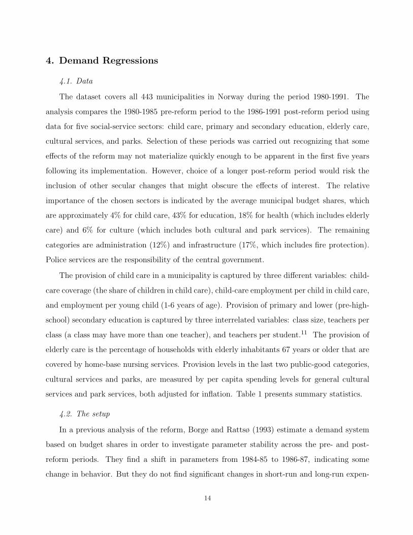
The dataset covers all 443 municipalities in Norway during the period 1980-1991. The

analysis compares the 1980-1985 pre-reform period to the 1986-1991 post-reform period using

data for five social-service sectors: child care, primary and secondary education, elderly care,

cultural services, and parks. Selection of these periods was carried out recognizing that some

effects of the reform may not materialize quickly enough to be apparent in the first five years

following its implementation. However, choice of a longer post-reform period would risk the

inclusion of other secular changes that might obscure the effects of interest. The relative

importance of the chosen sectors is indicated by the average municipal budget shares, which

are approximately 4% for child care, 43% for education, 18% for health (which includes elderly

care) and 6% for culture (which includes both cultural and park services). The remaining

categories are administration (12%) and infrastructure (17%, which includes fire protection).

Police services are the responsibility of the central government.

The provision of child care in a municipality is captured by three different variables: child-

care coverage (the share of children in child care), child-care employment per child in child care,

and employment per young child (1-6 years of age). Provision of primary and lower (pre-high-

school) secondary education is captured by three interrelated variables: class size, teachers per

class (a class may have more than one teacher), and teachers per student.11 The provision of

elderly care is the percentage of households with elderly inhabitants 67 years or older that are

covered by home-base nursing services. Provision levels in the last two public-good categories,

cultural services and parks, are measured by per capita spending levels for general cultural

services and park services, both adjusted for inflation. Table 1 presents summary statistics.

4.2. The setup

In a previous analysis of the reform, Borge and Rattsø (1993) estimate a demand system

based on budget shares in order to investigate parameter stability across the pre- and post-

reform periods. They find a shift in parameters from 1984-85 to 1986-87, indicating some

change in behavior. But they do not find significant changes in short-run and long-run expen-

14

diture elasticities or changes in the effects of demographic variables that are consistent with

the predicted effects of the reform. The present analysis, however, relies on the measures of

local service provision described above, which are more detailed than those in previous studies

and thus better able to capture the quantitative and qualitative aspects of the services. Note

that because most of these variables measure service levels rather than spending, estimation

of a demand system becomes infeasible.

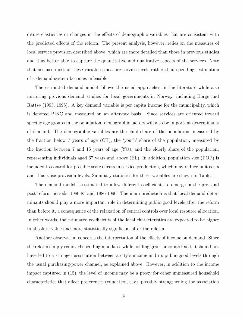
The estimated demand model follows the usual approaches in the literature while also

mirroring previous demand studies for local governments in Norway, including Borge and

Rattsø (1993, 1995). A key demand variable is per capita income for the municipality, which

is denoted PINC and measured on an after-tax basis. Since services are oriented toward

specific age groups in the population, demographic factors will also be important determinants

of demand. The demographic variables are the child share of the population, measured by

the fraction below 7 years of age (CH), the ‘youth’ share of the population, measured by

the fraction between 7 and 15 years of age (YO), and the elderly share of the population,

representing individuals aged 67 years and above (EL). In addition, population size (POP) is

included to control for possible scale effects in service production, which may reduce unit costs

and thus raise provision levels. Summary statistics for these variables are shown in Table 1.

The demand model is estimated to allow different coefficients to emerge in the pre- and

post-reform periods, 1980-85 and 1986-1990. The main prediction is that local demand deter-

minants should play a more important role in determining public-good levels after the reform

than before it, a consequence of the relaxation of central controls over local resource allocation.

In other words, the estimated coefficients of the local characteristics are expected to be higher

in absolute value and more statistically significant after the reform.

Another observation concerns the interpretation of the effects of income on demand. Since

the reform simply removed spending mandates while holding grant amounts fixed, it should not

have led to a stronger association between a city’s income and its public-good levels through

the usual purchasing-power channel, as explained above. However, in addition to the income

impact captured in (15), the level of income may be a proxy for other unmeasured household

characteristics that affect preferences (education, say), possibly strengthening the association

15

between provision levels and income.

Estimation of the pre- and post-reform demand coefficients is carried out within a single

regression model, where interaction terms allow different coefficients for the two periods while

the error variance is constrained to be the same across periods. The model, which facilitates

inter-period hypothesis tests on the coefficients, is

Sit = αt + Dpret ηpre

i + βpre1

log(PINCit) + βpre2

CHit + βpre3

YOit + βpre4

ELit + βpre5

log(POPit) +

(1 − Dpret )η

posti + β

post1

log(PINCit) + βpost2

CHit + βpost3

YOit + βpost4

ELit + βpost5

log(POPit) + εit

(16)

In (16), i denotes the municipality and t denotes the year, with the dummy variable Dpret

taking the value one when t is a pre-reform year and zero otherwise. Year fixed effects are

denoted by αt, while ηprei and ηpost

i give municipality fixed effects that may vary between the

periods. The other demand coefficients are also allowed to differ between the periods, and εit

is the error term.

Note that the inclusion of pre- and post-reform city fixed effects means that the impact

of the demand determinants is identified only through intraperiod, within-city variation in

the levels of the determinants. Small intertemporal variation in these covariates might then

militate against the emergence of significant demand effects.

4.3. Estimation results

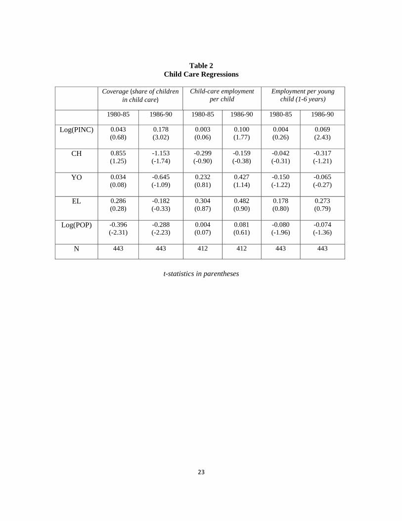
The estimated demand models for the three child-care measures are presented in Table 2.

The results show that child-care coverage was independent of income and the age composition

of the population before the reform. For the post-reform period, however, the estimates show

that income became a significant determinant of coverage, with the share of children in the

population becoming a marginally significant negative factor. This CH effect is consistent

with recent evidence from Borge and Rattsø (2008), who conclude using data from Denmark

that being part of a large cohort is a disadvantage in terms of child-care service levels.12 The

remaining columns of Table 2 show that the regressions for employment per child in child care

16

and employment per young child have mostly insignificant coefficients prior to the reform. But

both variables respond positively to income in the post-reform period, although one income

coefficient is only marginally significant.

To better judge whether the reform strengthened the link between service levels and the

determinants of demand in an overall sense, Table 3 provides several F tests, with the first

panel focusing on child care. The first column provides a test of the null hypothesis that the

vector of pre-reform coefficients equals the vector of post-reform coefficients. None of the F

statistics for the three child-care regressions allows rejection of this hypothesis, although the

statistic for coverage is marginally significant. Rather than testing for coefficient equality, a

different approach is to to ask whether the coefficient vector is zero, both before and after the

reform. As can be seen in the second and third columns, this hypothesis can be rejected in

both the pre- and post-reform cases for child-care coverage and employment per young child.

These results, which give a somewhat mixed picture of the effects of the reform, appear

to be driven by the population coefficients (meant to capture the effects of scale economies),

which are significant or nearly so in the pre-reform period. Since population can be viewed as a

less-central determinant of demand than the remaining demographic variables in the regression,

the last three columns of Table 3 carry out the previous F tests with the population coefficient

excluded. Now the picture provided by the tests is clearer. Coefficient equality across periods

is rejected for child-care coverage and nearly rejected for employment per young child. In

addition, the hypothesis that the pre-reform coefficient vector is zero cannot be rejected for

any of the child-care measures, while the post-reform vector is significantly different from zero

for coverage and employment per young child and marginally significant for the remaining

measure. Thus, this second set of tests suggests that the reform strengthened the link between

child-care services and the determinants of demand.

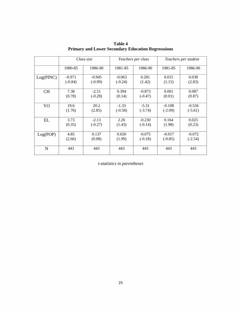
Table 4 shows the regression results for the three education measures. For the class-size

measure, the YO coefficient gains significance in the post-reform period and has the expected

positive sign (showing that more school-age children raise class sizes). For teachers per student,

higher income has a positive effect in the post-reform period but no pre-reform effect. A large

youth share reduces both teachers per class and per student in the post-reform period, with the

17

effect changing from insignificant to significant in the case of teachers per class. In addition, for

both service measures, YO’s coefficient magnitude is much larger in the post-reform period.13

Turning to the F tests in Table 3 and focusing on the tests that exclude the population

coefficient, pre- and post-reform coefficient equality is rejected for both teachers per class

and per student. In addition, whereas the coefficient vectors for all three service measures are

significantly different from zero in the post-reform period, two out of three are indistinguishable

from zero in the pre-reform period. Thus, as in the case of child care, the F tests suggest that

the reform strengthened the link between education services and the determinants of demand.

The elderly-care, culture and parks regressions are shown in Table 5. Somewhat surpris-

ingly, only one coefficient in the two elderly care regressions is significant, that of population

in the pre-reform period. In the case of cultural services, income becomes a significant deter-

minant of cultural spending in the post-reform period, with its effect much larger than the

marginally significant pre-reform impact. In addition, an increase in the elderly share reduces

cultural spending in the post-reform period, whereas no pre-reform effect exists. This negative

effect might seem counterintuitive, but it likely reflects competition for funds between cultural

services and services for the elderly in the local budget. In the park-spending regression, the

only significant effect is POP’s negative post-reform impact. Although both effects are only

marginally significant, a higher youth share raises park spending before and after the reform,

a natural outcome.

The F tests shown in the second half of the last panel of Table 3 do not allow rejection

of coefficient equality for any of the three services from Table 5. However, the post-reform

coefficient vector for cultural spending is significantly different from zero while the pre-reform

vector is not, suggesting that the reform strengthened the link between cultural spending and

the determinants of demand (despite the failure to reject coefficient equality). Note that neither

coefficient vector is significantly different from zero in the cases of elderly care and parks.

Overall, the results in Tables 2–5 offer support for the model’s prediction that local demo-

graphic characteristics should matter more in the determination of public-service levels after

the reform than before it. In six out of the nine cases in Table 5, the demographic variables

show no combined effect on service levels prior to the reform while exhibiting a statistically

18

significant impact after the reform. In particular, the F tests for child-care coverage and em-

ployment per young child, class size, teachers per class, and cultural spending show a nonzero

vector of demographics coefficients in the post-reform period, while failing in each case to reject

the null hypothesis of no demographic effects in the pre-reform period. The income variable,

which never has an effect on public-service provision prior to the reform, emerges after the

reform as a determinant of child-care coverage and employment per young child, teachers per

student, and cultural spending. In addition, larger cohort sizes (for children, youth, and el-

derly) lead to reductions in post-reform levels for some services, when effects were absent prior

to the reform. This pattern is seen for CH in child-care coverage (being marginally signifi-

cant), YO in class size and teachers per class, and EL in cultural spending. The results thus

suggest that local discretion granted under partial decentralization allows public-service levels

to respond to local demand.

5. The Reform’s Effect on Migration

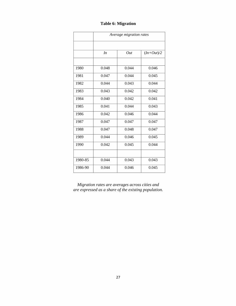
To test for a potential effect of the reform on intercity migration (a response to heightened

incentives for sorting of the population), yearly rates of in- and out-migration are computed

for each city in the sample and then averaged across cities. The results, which give migration

as a percentage of the existing population, are shown in Table 6, along with the combined

migration rate (the average of the in and out rates). All the migration rates lie between 4 and

5 percent, and the pre- and post-reform comparison at the bottom of the table suggests that

migration may have increased after the reform.

To provide a proper test, a panel regression is run for each of the three migration measures,

with the right-hand variables consisting of city fixed effects and a post-reform dummy variable.

The coefficient of this latter variable is positive and strongly significant in the combined and

out-migration regressions (t-statistics are 6.12 and 9.86 respectively), although it is insignificant

in the in-migration regression, matching the pattern seen in Table 5. Therefore, although

some other intertemporal cause for increased migration cannot be ruled out, these findings are

consistent with the existence of a greater incentive for population sorting after the reform, as

the theory would predict.14

19

To see whether increased migration is reflected in greater heterogeneity across cities, a

dissimilarity index is computed for the sample cities for each of the three age measures as well as

for all the measures together. Changes in city age distributions could perhaps capture greater

incentives for age-based sorting as some cities shift resources toward education (attracting

families with children) and others deemphasize education (becoming more attractive to the

elderly). The dissimilarity index, which uses the formula from Rhode and Strumpf (2003),

indicates the extent to which residents would need to move between cities in order to equalize

the age shares, thus being an increasing measure of intercity heterogeneity.15 The results are

mixed, showing greater post-reform heterogeneity for youth, less heterogeneity for the other

two categories, and a slight increase in overall post-reform heterogeneity. The absence of a

clearcut heterogeneity effect from the reform is not inconsistent, however, with its demonstrated

impact on migration. It could be argued that a longer time interval would be needed for greater

migration to notably affect city age compositions.

6. Conclusion

This paper provides an empirical test of a principal tenet of fiscal federalism: that spend-

ing discretion, when granted to localities, allows public-good levels to adjust in response to

local demands. The test is based on a simple model of partial fiscal decentralization, under

which earmarking of central transfers for particular uses is eliminated, allowing funds to be

spent according to local tastes. The model predicts that under partial decentralization, the

demographic characteristics of local jurisdictions should play a bigger role in determining the

levels of public goods after a decentralization reform than before. This prediction receives sup-

port from the paper’s empirical results, which show that local demand determinations matter

more after the 1986 Norwegian reform than before it, and that the reform may have increased

incentives for population sorting. These findings are important because they represent an

affirmation of a central, but seldom-tested, principle of public economics.

20

x*

z*

z le

vels

x le

vels

C

PD

FD

C

PD

FD

C =

cen

tral

izat

ion;

PD

= p

artia

l dec

entr

aliz

atio

n; F

D =

full

dece

ntra

lizat

ion

Figu

re 1

: Eff

ects

of D

ecen

traliz

atio

n

Type

2:

Type

1:

22

Table 1 Summary Statistics

Variables Before the reform After the reform All years

Child care

Coverage 0.261 (0.137)

0.408 (0.153)

0.328 (0.162)

Child-care employment per child 0.206 (0.073)

0.230 (0.067)

0.214 (0.072)

Employment per young child 0.051 (0.031)

0.095 (0.048)

0.071 (0.045)

Education

Class size 18.4 (3.47)

17.2 (3.37)

17.8 (3.47)

Teachers per class 1.80 (0.21)

2.08 (0.26)

1.94 (0.28)

Teachers per student 0.102 (0.025)

0.127 (0.034)

0.114 (0.032)

Elderly Care, Culture, and Parks

Elderly-care coverage 0.089 (0.057)

0.108 (0.058)

0.097 (0.058)

Cultural spending 390 (177)

505 (261)

436 (222)

Parks spending 32 (59)

29 (54)

31 (57)

Explanatory variables

Private income net of taxes per capita (PINC)

21,006 (2,472)

23,313 (2,417)

22,054 (2,703)

Share of children 0-6 years (CH)

0.093 (0.015)

0.089 (0.014)

0.091 (0.015)

Share of youths 7-15 years (YO)

0.148 (0.018)

0.130 (0.017)

0.140 (0.020)

Share of elderly 67 years and above (EL)

0.141 (0.037)

0.153 (0.039)

0.146 (0.038)

Population size (POP)

8,025 (14,678)

8,196 (15,046)

8,102 (14,845)

23

Table 2 Child Care Regressions

Coverage (share of children

in child care) Child-care employment

per child Employment per young

child (1-6 years)

1980-85 1986-90 1980-85 1986-90 1980-85 1986-90

Log(PINC) 0.043 (0.68)

0.178 (3.02)

0.003 (0.06)

0.100 (1.77)

0.004 (0.26)

0.069 (2.43)

CH 0.855 (1.25)

-1.153 (-1.74)

-0.299 (-0.90)

-0.159 (-0.38)

-0.042 (-0.31)

-0.317 (-1.21)

YO 0.034 (0.08)

-0.645 (-1.09)

0.232 (0.81)

0.427 (1.14)

-0.150 (-1.22)

-0.065 (-0.27)

EL 0.286 (0.28)

-0.182 (-0.33)

0.304 (0.87)

0.482 (0.90)

0.178 (0.80)

0.273 (0.79)

Log(POP) -0.396 (-2.31)

-0.288 (-2.23)

0.004 (0.07)

0.081 (0.61)

-0.080 (-1.96)

-0.074 (-1.36)

N 443 443 412 412 443 443

t-statistics in parentheses

24

Table 3 F-tests

All coefficients All coefficients except population

size

Equality before and

after

Jointly zero before

Jointly zero after

Equality before

and after

Jointly zero before

Jointly zero after

Child care

Coverage 1.90 (0.094)

3.14 (0.009)

5.59 (0.000)

2.23 (0.065)

0.053 (0.716)

3.39 (0.001)

Child-care employment per child

0.52 (0.759)

0.72 (0.612)

1.91 (0.092)

0.57 (0.688)

0.084 (0.498)

1.64 (0.165)

Employment per young child

1.55 (0.174)

3.51 (0.004)

5.29 (0.000)

1.78 (0.131)

0.74 (0.562)

2.84 (0.024)

Education

Class size 1.07 (0.379)

4.36 (0.001)

3.05 (0.010)

0.19 (0.944)

2.19 (0.069)

3.52 (0.008)

Teachers per class 3.01 (0.011)

1.60 (0.159)

3.86 (0.011)

2.49 (0.042)

1.51 (0.199)

4.12 (0.003)

Teachers per student 7.41 (0.000)

4.85 (0.000)

15.45 (0.000)

8.73 (0.000)

2.81 (0.025)

14.99 (0.000)

Elderly Care, Culture, and Parks

Elderly-care coverage 0.97 (0.434)

1.54 (0.175)

0.87 (0.504)

1.19 (0.313)

1.51 (0.197)

0.69 (0.599)

Culture 0.85 (0.518)

3.94 (0.002)

9.69 (0.000)

1.04 (0.388)

1.41 (0.229)

7.29 (0.000)

Parks 1.92 (0.089)

0.69 (0.628)

3.54 (0.004)

0.40 (0.812)

0.76 (0.549)

1.59 (0.176)

F statistics with p-values in parentheses

25

Table 4 Primary and Lower Secondary Education Regresssions

Class size Teachers per class Teachers per student

1980-85 1986-90 1981-85 1986-90 1981-85 1986-90

Log(PINC) -0.971 (-0.84)

-0.945 (-0.99)

-0.063 (-0.24)

0.281 (1.42)

0.015 (1.15)

0.038 (2.83)

CH 7.38 (0.78)

-2.51 (-0.28)

0.394 (0.14)

-0.873 (-0.47)

0.001 (0.01)

0.087 (0.87)

YO 19.6 (1.76)

20.2 (2.85)

-1.33 (-0.58)

-5.31 (-3.74)

-0.108 (-2.09)

-0.556 (-5.61)

EL 3.73 (0.35)

-2.13 (-0.27)

2.26 (1.43)

-0.230 (-0.14)

0.164 (1.98)

0.025 (0.23)

Log(POP) 4.85 (2.66)

0.137 (0.08)

0.650 (1.99)

-0.075 (-0.18)

-0.017 (-0.85)

-0.072 (-2.54)

N 443 443 443 443 443 443

t-statistics in parentheses

26

Table 5 Elderly-Care, Culture, and Parks Regressions

Elderly-Care

Coverage Cultural spending per

capita Parks spending per

capita

1980-85 1986-89 1980-85 1986-89 1980-85 1986-89

Log(PINC) -0.026 (-0.59)

-0.015 (-0.29)

199.7 (1.70)

363.1 (3.58)

-9.34 (-0.32)

-4.21 (-0.17)

CH -0.058 (-0.16)

-0.261 (-0.72)

-806.1 (-1.20)

-1466.0 (-1.04)

106.4 (0.47)

-67.3 (-0.32)

YO 0.571 (1.48)

-0.296 (-0.99)

-374.8 (-0.55)

420.6 (0.35)

445.3 (1.91)

411.4 (1.84)

EL -0.870 (-1.70)

-0.471 (-1.00)

-775.9 (-0.65)

-3273.3 (-2.44)

107.9 (0.37)

-282.6 (-1.46)

Log(POP) -0.173 (-2.32)

-0.123 (-1.69)

-575.8 (-2.57)

-707.2 (-2.94)

30.9 (0.72)

-116.4 (-2.62)

N 443 443 443 443 443 443

t-statistics in parentheses; note that, due to data limitations, the post-reform

period for these services does not include 1990

27

Table 6: Migration

Average migration rates

In Out (In+Out)/2

1980 0.048 0.044 0.046

1981 0.047 0.044 0.045

1982 0.044 0.043 0.044

1983 0.043 0.042 0.042

1984 0.040 0.042 0.041

1985 0.041 0.044 0.043

1986 0.042 0.046 0.044

1987 0.047 0.047 0.047

1988 0.047 0.048 0.047

1989 0.044 0.046 0.045

1990 0.042 0.045 0.044

1980-85 0.044 0.043 0.043

1986-90 0.044 0.046 0.045

Migration rates are averages across cities and are expressed as a share of the existing population.

28

Table 7: Dissimilarity index for share of children (CH), youths (YO), elderly (EL) and total for all three groups

Year CH YO EL Total

1980 0.059 0.052 0.115 0.075

1981 0.061 0.052 0.115 0.076

1982 0.062 0.052 0.114 0.076

1983 0.064 0.052 0.113 0.076

1984 0.064 0.052 0.112 0.077

1985 0.064 0.052 0.113 0.077

1986 0.061 0.053 0.113 0.077

1987 0.060 0.055 0.113 0.078

1988 0.057 0.056 0.112 0.078

1989 0.054 0.058 0.111 0.077

1990 0.052 0.059 0.109 0.077

1980-85 0.062 0.052 0.114 0.076

1986-90 0.057 0.056 0.112 0.077

References

Ahlin, A., Mork, E., 2008. Effects of decentralization on school resources. Economics of

Education Review 27, 276-284.

Arzaghi, M., Henderson, J.V., 2005. Why countries are fiscally decentralizing. Journal

of Public Economics 89, 1157-1189.

Banzhaf, S., Walsh, R.P., 2008. Do people vote with their feet? An empirical test ofTiebout’s mechanism. American Economic Review 98, 843-863.

Barankay, I., Lockwood, B., 2007. Decentralization and the productive efficiency ofgovernment: Evidence from Swiss cantons. Journal of Public Economics 91, 1197-1218.

Bayer, P., Timmins, C., 2007. Estimating equilibrium models of sorting across locations.Economic Journal 117. 353-74.

Besley, T., Coate, S., 2003. Centralized vs. decentralized provision of local public goods:A political economy analysis. Journal of Public Economics 87, 2611-2637.

Borge, L.-E., Rattsø, J., 1993. Dynamic responses to changing demand: A model of thereallocation process in small and large municipalities in Norway. Applied Economics 25,589-598.

Borge, L.-E., Rattsø, J., 1995. Demographic shift, relative costs and the allocation oflocal public consumption in Norway. Regional Science and Urban Economics 25, 705-726.

Borge, L.-E., Rattsø, J., 2002. Spending growth with vertical fiscal imbalance: Decen-tralized government spending in Norway 1880-1990. Economics and Politics 14, 351-373.

Borge, L.-E., Rattsø, J., 2008. Generational conflict and the disadvantage of being partof a large cohort: Empirical analysis of demography and welfare service production inDenmark. CESifo Working paper 2223.

Brueckner, J.K., 2004. Fiscal decentralization with distortionary taxation: Tiebout vs. taxcompetition. International Tax and Public Finance 11, 133-53.

Brueckner, J.K., 2009. Partial fiscal decentralization. Regional Science and Urban Eco-

nomics 39, 23-32.

Eberts, R., Gronberg, T.J., 1981. Jurisdictional homogeneity and the Tiebout hypothesis.Journal of Urban Economics 10, 227-239.

29

Faguet, J.-P., 2004. Does decentralization increase government responsiveness to localneeds? Evidence from Bolivia. Journal of Public Economics 88, 867-893.

Hatfield, J.W., Padro i Miguel, G., 2011. A political economy theory of partial decen-tralization. Journal of the European Economic Association, forthcoming.

Jametti, M., Joanis, M., 2011. Electoral competition as a determinant of fiscal decentral-ization. Unpublished paper, University of Sherbrooke, Canada.

Lockwood, B., 2002. Distributive politics and the costs of centralization. Review of Eco-

nomic Studies 69, 313-337.

Lorz, O., Willmann, G., 2005. On the endogenous allocation of decision powers in federalstructures. Journal of Urban Economics 57, 242-257.

Lotz, J., 1998. Local government reforms in the Nordic countries, theory and practice. InJ. Rattso (Ed.), Fiscal Federalism and State-Local Finance: The Scandinavian Approach,Edward Elgar, Cheltenham, UK.

Oates, W.E., 1969. The effects of property taxes and local public spending on propertyvalues: An empirical study of tax capitalization and the Tiebout hypothesis. Journal of

Political Economy 77, 957-71.

Oates, W.E., 1972. Fiscal Federalism. Harcourt Brace, New York.

Pack, H., Pack, J., 1978. Metropolitan fragmentation and local public expenditure. Na-

tional Tax Journal 31, 349-362.

Panizza, U., 1999. On the determinants of fiscal centralization: Theory and evidence. Journal

of Public Economics 74, 97-139.

Peralta, S., 2012. Partial fiscal decentralization, local elections, and accountability. Unpub-lished paper, Nova School of Business and Economics, Lisbon.

OECD, 1999. Taxing Powers of State and Local Governments. Organization for EconomicCooperation and Development, Paris.

Rattsø, J., 2004. Fiscal adjustment under centralized federalism: Empirical evaluation ofthe response to budgetary shocks. Finanzarchiv 60, 240-261.

Rodden, J., Eskeland, G., Litvack, J., 2003. Fiscal Decentralization and the Challenge

of the Hard Budget Constraint. MIT Press, Cambridge, Mass.

Rhode, P.W., Strumpf, K.S., 2003. Assessing the importance of Tiebout sorting: Local

30

heterogeneity from 1850 to 1990. American Economic Review 93, 1648-77.

Schwager, R., 1999. Administrative federalism and a central government with regionallybased preferences, International Tax and Public Finance 6, 165-189.

Shah, A., 2004. Fiscal decentralization in developing and transition economies, unpublishedpaper, World Bank.

Shah, A., Shah, S., 2006. The new vision of local governance and the evolving roles of localgovernments, unpublished paper, World Bank.

Sigman, H., 2007. Decentralization and environmental quality: An international analysis ofwater pollution. National Bureau of Economic Research Working Paper #13098.

Tiebout, C.M., 1956. A pure theory of local expenditures. Journal of Political Economy 64,416-424.

Wildasin, D.E., 1986. Urban Public Finance. Harwood Academic Publishers, Chur, Switzer-land.

Zhuravskaya, E., 2000. Incentives to provide local public goods: Fiscal federalism, Russianstyle. Journal of Public Economics 76, 337-368.

31

Footnotes

∗We thank Spencer Banzhaf, Jon Fiva, Arnt Ove Hopland, Kangoh Lee, Albert Sole-Olle, WillStrange, and several referees for helpful comments. We are also grateful to the followingdiscussants for comments: John Ashworth (“End of Federalism” conference at WZB inBerlin, 2012), Norman Gemmell (LAV #11 conference in Marseille, 2012), Federico Revelli(“Workshop on Fiscal Federalism” in Barcelona, 2013), and Enlinson Mattos (IIPF congressin Taormina, 2013). We also thank audiences at the 2013 EEA conference in Gothenburgand the Einaudi Institute of Economics and Finance for feedback.

1For example, figures presented by Shah and Shah (2006) show that, in a sample of tenlower-income countries, local governments relied on intergovernmental transfers for 51% oftheir revenue, in contrast to a smaller transfer share of 34% for OECD countries. In a largersample of developing countries analyzed by Shah (2004), 42% of subnational revenue (localand provincial) came from transfers.

2Although the Shah studies cited in footnote 1 do not present evidence on tax autonomy forthe sample countries, a separate OECD study (1999) shows that, for one sample country(Mexico), subnational governments had effective control over only 14% of their tax revenue,with this limited control enjoyed only at the state rather than local level.

3This decoupling allows public-good provision to respond under partial decentralization toheterogeneity in the demands for z despite a common transfer level for all localities. Theresponse is narrower, however, than under full decentralization.

4Sigman (2007) offers a test for the effects of decentralization that does not rely on a naturalexperiment. Her empirical results show that variation in environmental quality is higherwithin federalist countries than within non-federal states, evidently reflecting variation inthe restrictiveness of local environmental policies within the former set of countries.

5With full decentralization, jurisdictions in his model choose both the investment level inindividual public projects and the number of projects to implement, in a setting with inter-jurisdictional spillovers. The central government can improve the outcome by specifying thelevel of project investment while still allowing localities to choose the number of projectsundertaken, a partial-decentralization outcome that shares the spirit of the current approach.

6It does so because spending is then fixed at the level of the central transfer regardless ofwhether the uncertain unit cost of the public good turns out to be high or low (rather thanadjusting to reflect this cost). As a result, rent-seeking politicians who wish to masqueradeas benevolent can more easily extract rents under partial decentralization without revealing

32

their type. While this conclusion affirms the superiority of full decentralization, Brueckner(2009) (in a variant of his basic model) offers a different result by showing that partialdecentralization instead limits the options of rent-seekers, making it potentially superior tofull decentralization.

7While local governments use nonredistributive and nondistortionary head taxes in a desireto avoid tax competition, a redistributive capital tax, which also distorts the economy bydepressing capital supply, funds central provision of public goods. Facing a tradeoff betweenefficiency and redistribution in the choice of local versus central provision, voters choose theoptimal share of public goods to be provided locally, thus determining the extent of partialfiscal decentralization. Panizza (1999) and Jametti and Joanis (2011) use similar models inempirically oriented papers.

8For example, Rodden, Eskeland and Litvack (2003) offer a set of country studies addressingvarious issues of fiscal discipline in centralized systems. In the Norwegian context, Borge andRattsø (2002) and Rattsø (2004) analyze fiscal adjustment within that country’s centralizedfiscal structure. Barankay and Lockwood (2007) analyze the impact of decentralizationon governmental productive efficiency, using data for Swiss cantons with different degreesof decentralization. Zhuravskaya (2000) studies private business formation across Russiancities with different degrees of fiscal discretion.

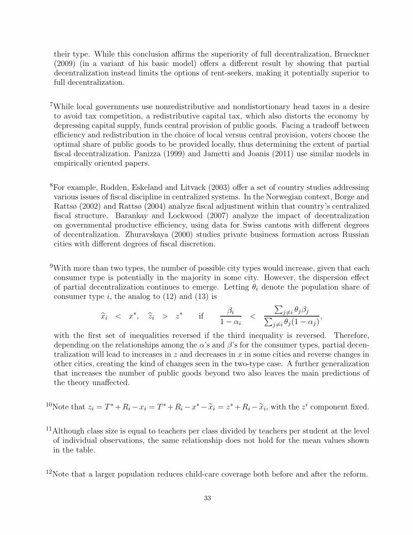
9With more than two types, the number of possible city types would increase, given that eachconsumer type is potentially in the majority in some city. However, the dispersion effectof partial decentralization continues to emerge. Letting θi denote the population share ofconsumer type i, the analog to (12) and (13) is

xi < x∗, zi > z∗ ifβi

1 − αi<

∑j 6=i θjβj∑

j 6=i θj(1 − αj),

with the first set of inequalities reversed if the third inequality is reversed. Therefore,depending on the relationships among the α’s and β’s for the consumer types, partial decen-tralization will lead to increases in z and decreases in x in some cities and reverse changes inother cities, creating the kind of changes seen in the two-type case. A further generalizationthat increases the number of public goods beyond two also leaves the main predictions ofthe theory unaffected.

10Note that zi = T ∗+Ri −xi = T ∗+Ri −x∗− xi = z∗ +Ri − xi, with the zi component fixed.

11Although class size is equal to teachers per class divided by teachers per student at the levelof individual observations, the same relationship does not hold for the mean values shownin the table.

12Note that a larger population reduces child-care coverage both before and after the reform.

33

13A significantly positive elderly-share effect, which is hard to interpret, exists in the pre-reform period for teachers per student, but it disappears following the reform. Similarly,a significantly positive population effect exists prior to the reform for teachers per class,disappearing after it. These changes, which unfortunately run counter to the predictions,contribute to the significance of the F statistics.

14Table 5 presents unweighted migration rates, where the rates are not weighted by city popu-lations. While weighted rates do not replicate the apparent post-reform migration increase,the regression results, being based on individual city populations and including city fixedeffects, give the clearest picture.

15The number of people needing to move is expressed relative to the number who would haveto move to equalize age shares if the population were completely segregated by age.

34