Embed Size (px)
Citation preview
Electronic Journal of StatisticsISSN: 1935-7524arXiv: math.PR/0000000
Partial Information Framework: Model-Based Aggregationof Estimates from Diverse Information Sources∗
Ville A. SatopaaDepartment of Technology and Operations Management, INSEAD, Fontainebleau, France
e-mail: [email protected]
Shane T. JensenDepartment of Statistics, The Wharton School of the University of Pennsylvania, Philadelphia, PA 19104-6340, USA
e-mail: [email protected]
Robin PemantleDepartment of Mathematics, University of Pennsylvania, Philadelphia, PA 19104-6395, USA
e-mail: [email protected]
Lyle H. UngarDepartment of Computer and Information Science, University of Pennsylvania, Philadelphia, PA 19104-6309, USA
e-mail: [email protected]
Summary: Prediction polling is an increasingly popular form of crowdsourcing in which multiple participantsestimate the probability or magnitude of some future event. These estimates are then aggregated into a singleforecast. Historically, randomness in scientific estimation has been generally assumed to arise from unmeasuredfactors which are viewed as measurement noise. However, when combining subjective estimates, heterogeneitystemming from differences in the participants’ information is often more important than measurement noise. Thispaper formalizes information diversity as an alternative source of such heterogeneity and introduces a novel mod-eling framework that is particularly well-suited for prediction polls. A practical specification of this frameworkis proposed and applied to the task of aggregating probability and point estimates from two real-world predic-tion polls. In both cases our model outperforms standard measurement-error-based aggregators, hence providingevidence in favor of information diversity being the more important source of heterogeneity.
MSC 2010 subject classifications: Primary 62A01, 62B99; secondary 62P15.Keywords and phrases: Expert belief, Forecast heterogeneity, Judgmental forecasting, Model averaging, Noisereduction, Unsupervised learning.
Contents
1 INTRODUCTION . . . . . . . . . . . . . . . . . . . . . . . . . . . . . . . . . . . . . . . . . . . . . 22 MODEL-BASED AGGREGATION . . . . . . . . . . . . . . . . . . . . . . . . . . . . . . . . . . . . 5
2.1 Bias and Noise . . . . . . . . . . . . . . . . . . . . . . . . . . . . . . . . . . . . . . . . . . . . 52.2 Partial Information Framework . . . . . . . . . . . . . . . . . . . . . . . . . . . . . . . . . . . . 5
2.2.1 General Framework . . . . . . . . . . . . . . . . . . . . . . . . . . . . . . . . . . . . . . 5∗This research was supported by a research contract to the University of Pennsylvania and the University of California from the Intelli-
gence Advanced Research Projects Activity (IARPA) via the Department of Interior National Business Center contract number D11PC20061.The U.S. Government is authorized to reproduce and distribute reprints for Government purposes notwithstanding any copyright annota-tion thereon. Disclaimer: The views and conclusions expressed herein are those of the authors and should not be interpreted as necessarilyrepresenting the official policies or endorsements, either expressed or implied, of IARPA, DoI/NBC, or the U.S. Government.
1imsart-ejs ver. 2014/10/16 file: PIF170925.tex date: September 25, 2017

V. A. Satopaa et al./Partial Information Framework 2
2.2.2 Gaussian Partial Information Model . . . . . . . . . . . . . . . . . . . . . . . . . . . . . 82.3 Previous Work on Model-Based Aggregation . . . . . . . . . . . . . . . . . . . . . . . . . . . . 9
2.3.1 Interpreted Signal Framework . . . . . . . . . . . . . . . . . . . . . . . . . . . . . . . . 92.3.2 Measurement Error Framework . . . . . . . . . . . . . . . . . . . . . . . . . . . . . . . 10
3 MODEL ESTIMATION . . . . . . . . . . . . . . . . . . . . . . . . . . . . . . . . . . . . . . . . . . 103.1 General Estimation Problem . . . . . . . . . . . . . . . . . . . . . . . . . . . . . . . . . . . . . 103.2 Maximum Likelihood Estimator . . . . . . . . . . . . . . . . . . . . . . . . . . . . . . . . . . . 113.3 Least Squares Estimator . . . . . . . . . . . . . . . . . . . . . . . . . . . . . . . . . . . . . . . 123.4 Conditional Validation . . . . . . . . . . . . . . . . . . . . . . . . . . . . . . . . . . . . . . . . 13
4 SYNTHETIC DATA ANALYSIS . . . . . . . . . . . . . . . . . . . . . . . . . . . . . . . . . . . . . . 145 APPLICATIONS . . . . . . . . . . . . . . . . . . . . . . . . . . . . . . . . . . . . . . . . . . . . . . 17
5.1 Probability Forecasts of Binary Outcomes . . . . . . . . . . . . . . . . . . . . . . . . . . . . . . 175.1.1 Dataset . . . . . . . . . . . . . . . . . . . . . . . . . . . . . . . . . . . . . . . . . . . . 175.1.2 Model Specification and Aggregation . . . . . . . . . . . . . . . . . . . . . . . . . . . . 175.1.3 Information Diversity . . . . . . . . . . . . . . . . . . . . . . . . . . . . . . . . . . . . . 20
5.2 Point Forecasts of Continuous Outcomes . . . . . . . . . . . . . . . . . . . . . . . . . . . . . . . 215.2.1 Dataset . . . . . . . . . . . . . . . . . . . . . . . . . . . . . . . . . . . . . . . . . . . . 215.2.2 Model Specification and Aggregation . . . . . . . . . . . . . . . . . . . . . . . . . . . . 21
6 DISCUSSION . . . . . . . . . . . . . . . . . . . . . . . . . . . . . . . . . . . . . . . . . . . . . . . . 22A Finding µ∗ for Psd(· : κ) . . . . . . . . . . . . . . . . . . . . . . . . . . . . . . . . . . . . . . . . . . 24
1. INTRODUCTION
Past literature has distinguished two types of polling: prediction and opinion polling. In broad terms, an opinionpoll is a survey of public opinion, whereas a prediction poll involves multiple agents collectively predicting thevalue of some quantity of interest (Goel et al., 2010; Mellers et al., 2014). For instance, consider a presidentialelection poll. An opinion poll typically asks the voters who they will vote for. A prediction poll, on the otherhand, could ask which candidate they think will win in their state. A liberal voter in a dominantly conservativestate is likely to answer differently to these two questions. Even though opinion polls have been the dominantfocus historically, prediction polls have become increasingly popular in the recent years, due to modern socialand computer networks that permit the collection of a large number of responses both from human and machineagents. This has given rise to crowdsourcing platforms, such as MTurk and Witkey, and many companies, suchas Myriada, Lumenogic, and Inkling, that have managed to successfully capitalize on the benefits of collectivewisdom.
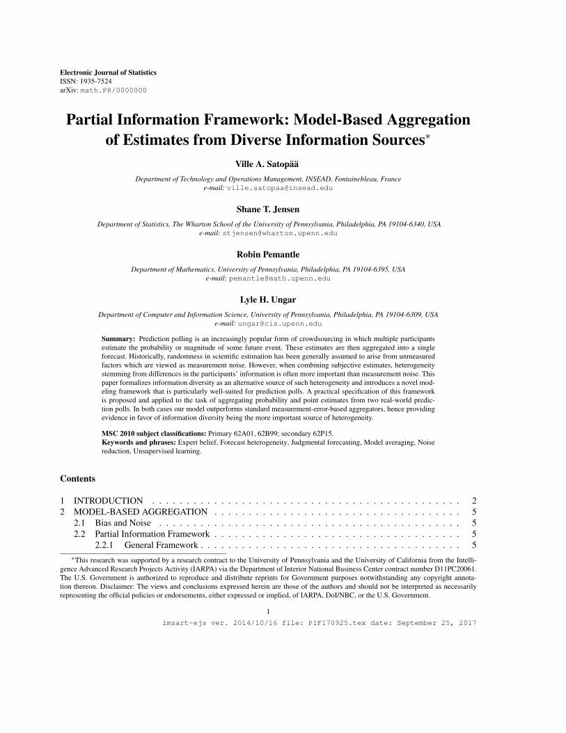
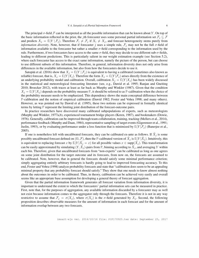
We introduce statistical methodology designed specifically for the rapidly growing practice of predictionpolling. The methods are illustrated on real-world data involving two common types of responses, namely prob-ability and point forecasts. The probability forecasts were collected by the Good Judgment Project (GJP) (Ungaret al. 2012; Mellers et al. 2014) as a means to estimate the likelihoods of international political future eventsdeemed important by the Intelligence Advanced Research Projects Activity (IARPA). Since its initiation in 2011,the project has recruited thousands of forecasters to make probability estimates and update them whenever theyfelt the likelihoods had changed. To illustrate, Figure 1 shows the forecasts for one of these events. This exam-ple involves 522 forecasters making a total of 1, 669 predictions between 30 July 2012 and 30 December 2012when the event finally resolved as “No” (represented by the red line at 0.0). The point forecasts for our secondapplication were collected by Moore and Klein (2008) who recruited 416 undergraduates from Carnegie Mellon
imsart-ejs ver. 2014/10/16 file: PIF170925.tex date: September 25, 2017

V. A. Satopaa et al./Partial Information Framework 3
Sep Nov Jan
0.0
0.2
0.4
0.6
0.8
1.0
Pro
babi
lity
For
ecas
t
Date
Fig 1: Probability forecasts of the event “Will Moody’sissue a new downgrade on the long-term ratings forany of the eight major French banks between 30 July2012 and 31 December 2012?” The points have beenjittered slightly to make overlaps visible.
0 5 10 15 200
5010
015
020
025
0P
oint
For
ecas
t (P
ound
s)
Person
Fig 2: Point forecasts of the weights of 20 differentpeople. The boxplots have been sorted to increase inthe true weights (red dots). Some extreme values wereomitted for the sake of clarity.
University to guess the weights of 20 people based on a series of pictures. The responses are illustrated in Fig-ure 2 that shows the boxplots of the forecasters’ guesses for each of the 20 people. The red dots represent thecorresponding true weights.
Once the predictions have been collected, they are typically combined into a single consensus forecast for thesake of decision-making and improved accuracy. Unfortunately, this can be done in many different ways, and thefinal combination rule can largely determine the out-of-sample performance. The past literature distinguishes twobroad approaches to forecast aggregation: empirical aggregation and model-based aggregation. Empirical aggre-gation is by far the more widely studied approach; see, e.g., stacking (Breiman, 1996), Bayes model averaging(Raftery et al., 1997), linear opinion pools (DeGroot and Mortera, 1991), and extremizing aggregators (Ranjanand Gneiting, 2010; Satopaa et al., 2014a,b). This approach is akin to machine learning in a sense that it firstlearns the aggregator based on a training set of past forecasts of known outcomes and then uses that aggregator tocombine future forecasts of unknown outcomes. Unfortunately, constructing such a training set requires a lot ofeffort and time on behalf of the forecasters and the polling agent. In practice a typical prediction poll uses a singlequestionnaire that simultaneously inquires about the participants’ predictions of one or more unknown outcomes.The result is a dataset consisting only of forecasts and no outcomes, which means that empirical aggregationcannot be applied.
Fortunately, model-based aggregation can be performed even when prior knowledge of outcomes is not avail-able. This approach first proposes a plausible probability model for the source of heterogeneity among the fore-casts, that is, for how and why the forecasts differ from the target outcome. Under this assumed forecast-outcome
imsart-ejs ver. 2014/10/16 file: PIF170925.tex date: September 25, 2017

V. A. Satopaa et al./Partial Information Framework 4
link, it is then possible to construct an optimal aggregator that can be applied directly to the forecasts withoutlearning the aggregator first from a separate training set. Given this broad applicability, the current paper focusesonly on the model-based approach. In particular, outcomes are not assumed available for aggregation at any pointin the paper. Instead, aggregation is performed solely based on forecasts, leaving all empirical techniques welloutside the scope of the paper.
Historically, potentially due to early forms of data collection, model-based aggregation has considered mea-surement error as the main source of forecast heterogeneity (Hong and Page, 2009; Lobo and Yao, 2010). Thischoice motivates aggregators with central tendency such as the (weighted) average, median, and so on. Intuitively,measurement error may be reasonable in modeling repeated estimates from a single instrument. However, it is un-likely to hold in prediction polling, where the estimates arise from multiple, often widely different sources. In fact,a strict convex combination is never the optimal aggregator (in terms of the expected quadratic and many otherloss functions) under any joint distribution of the outcome and its (at least two different) forecasts (Dawid et al.,1995; Ranjan and Gneiting, 2010; Satopaa, 2017). This questions the role of measurement error in model-basedaggregation and highlights the need for a different source of forecast heterogeneity.
Hong and Page (2009) offer an alternative source called “cognitive diversity.” This model assumes that differ-ent predictions arise from differing interpretation procedures. For example, consider two forecasters who visit acompany and predict its future revenue. Even though the forecasters receive and possibly even use the exact sameinformation, they may interpret it differently and hence end up reporting different forecasts. Therefore forecastheterogeneity stems from differences in the forecasters’ information and how they interpret it. Hong and Page(2009) use this source in theoretical models with known interpretations to illustrate the behavior of cognitivelydiverse forecasters. They do not discuss estimation or modeling of real-world predictions. In fact, it is not evenclear how or if the forecasters’ interpretations can be estimated from the predictions.
Therefore, to bring information-driven heterogeneity to real-world applications, we introduce information di-versity. This differs from cognitive diversity by excluding the interpretation component and hence explainingvariation purely in terms of differences in the information used by the forecasters. It forms the basis of a novelmodeling framework called the partial information framework. Satopaa et al. (2016) introduced the theory be-hind the first version of this framework; though their specification only applies to probability forecasts and makesstructural assumptions that hinder empirical applications. Similarly to Hong and Page (2009), their focus is ontheory instead of practice. Consequently, the framework has remained rather abstract.
The current paper changes that by offering an empirical counterpart to Satopaa et al. (2016). In particular, thispaper separates itself from past work with the following contributions:
i) Section 2 introduces a new specification of the framework. This involves fewer assumptions, suits differenttypes of outcome-forecast pairs (instead of just probability forecasts of binary outcomes as in Satopaa et al.2016), and is more amenable for real-world applications. The new specification allows the decision-maker tobuild models that motivate and describe explicit joint distributions for the outcome and forecasts. The optimalaggregator under each joint distribution then serves as a more principled model-based alternative to the usual(weighted) average or median.
ii) Section 3 develops a general procedure for estimating partial information models. This requires a significantamount of innovation for several reasons. First, the forecasters’ information is captured in their covariancematrix. This matrix, that shows each forecaster’s information and also the information overlap between anytwo forecasters, must satisfy some physically inspired constraints. For instance, if two forecasters know 60%of all information, then their information must overlap by at least 20% of all information. Of course, the finalcovariance matrix must represent an arrangement of information that is simultaneously feasible for all theforecasters. Second, the number of unknown parameters is
(N+12
), where N is the number of forecasters.
Standard optimization techniques can then solve this problem for a maximum of about 45 forecasters – anumber that is far too small for many real-world prediction polls. Third, prediction polls often have more
imsart-ejs ver. 2014/10/16 file: PIF170925.tex date: September 25, 2017

V. A. Satopaa et al./Partial Information Framework 5
forecasters than unknown outcomes. This is a high-dimensional setting where covariance matrix estimationis known to be challenging.
iii) Even though in the past others have modeled variation in the forecasters’ information (see Section 2.3.1), tothe best of our knowledge, no previous work has developed estimation methodology and hence been able tosuccessfully apply such models to real-world data. This paper, however, applies our specification to two real-world prediction polls. In particular, Section 5 illustrates how the forecasters’ information can be measuredand used in aggregation. Overall, the resulting partial information aggregators achieve a noticeable perfor-mance improvement over the common measurement-error-based aggregators, suggesting that informationdiversity is the more appropriate model of forecast heterogeneity.
The paper is structured as follows. Section 2 describes the general partial information framework, introduces apractical specification of the framework, and gives a brief review of previous work on model-based aggregation.Section 3 derives the estimation procedure. Sections 4 and 5 illustrate specific models on synthetic data and real-world forecasts from the two prediction polls discussed above. Section 6 concludes with a summary and discussionof future research.
2. MODEL-BASED AGGREGATION
2.1. Bias and Noise
Consider N forecasters and suppose forecaster j predicts Xj for some quantity of interest Y . For instance, in ourweight estimation example Y is the true weight of a person and Xj is the guess given by the jth undergraduate.In our probability forecasting application, on the other hand, Y is binary, reflecting whether the event happens ornot, and Xj ∈ [0, 1] is a probability forecast for its occurrence. This section, however, avoids such applicationspecific choices and instead treats Y and Xj as generic random variables.
The prediction Xj is nothing but an estimator of Y . Therefore, as is the case with all estimators, its deviationfrom the truth can be broken down into two components: bias and noise. On the theoretical level, these two compo-nents can be separated and hence are often addressed by different mechanisms. This suggests a two-step approachto forecast aggregation: i) eliminate any bias in the forecasts, and ii) combine the unbiased forecasts. In this paperbias reduction is mentioned occasionally. The main focus, however, is on noise reduction and hence on developingmethodology for the second step in forecast aggregation. Section 2.2 begins this discussion by describing our newframework for the noise component. Section 2.3 then compares this to previous frameworks. These frameworksmake different assumptions about the way the forecasts relate to the outcome and hence motivate very differentclasses of model-based aggregators.
2.2. Partial Information Framework
2.2.1. General Framework
The partial information framework assumes that Y is measurable under some probability space (Ω,F ,P). Theprobability measure P provides a non-informative yet proper prior on Y and reflects the basic information knownto all forecasters. Such a prior has been discussed extensively in the economics and game theory literature whereit is usually known as the common prior (see, e.g., Morris 1995). Even though this is a substantive assumption inthe framework, specifying a prior distribution cannot be avoided as long as the model depends on a probabilityspace. How the prior is incorporated depends on the problem context: it can be chosen by the decision-maker,computed based on past observations of Y , or estimated from the forecasts.
imsart-ejs ver. 2014/10/16 file: PIF170925.tex date: September 25, 2017
V. A. Satopaa et al./Partial Information Framework 6
The principal σ-field F can be interpreted as all the possible information that can be known about Y . On top ofthe basic information reflected in the prior, the jth forecaster uses some personal partial information set Fj ⊆ Fand predicts Xj = E(Y | Fj). Therefore Fi 6= Fj if Xi 6= Xj , and forecast heterogeneity stems purely frominformation diversity. Note, however, that if forecaster j uses a simple rule, Fj may not be the full σ-field ofinformation available to the forecaster but rather a smaller σ-field corresponding to the information used by therule. Furthermore, if two forecasters have access to the same σ-field, they may decide to use different sub-σ-fields,leading to different predictions. This is particularly salient in our weight estimation example (see Section 5.2),where each forecaster has access to the exact same information, namely the picture of the person, but can chooseto use different subsets of this information. Therefore, in general, information diversity does not only arise fromdifferences in the available information, but also from how the forecasters decide to use it.
Satopaa et al. (2016) show that Xj = E(Y | Fj) is equivalent to having a calibrated (sometimes also known asreliable) forecast, that is,Xj = E(Y |Xj). Therefore the formXj = E(Y |Fj) arises directly from the existence ofan underlying probability model and calibration. Overall, calibration Xj = E(Y |Xj) has been widely discussedin the statistical and meteorological forecasting literature (see, e.g., Dawid et al. 1995; Ranjan and Gneiting2010; Broecker 2012), with traces at least as far back as Murphy and Winkler (1987). Given that the conditionXj = E(Y |Xj) depends on the probability measure P, it should be referred to as P-calibration when the choice ofthe probability measure needs to be emphasized. This dependency shows the main conceptual difference betweenP-calibration and the notion of empirical calibration (Dawid 1982; Foster and Vohra 1998; and many others).However, as was pointed out by Dawid et al. (1995), these two notions can be expressed in formally identicalterms by letting P represent the limiting joint distribution of the forecast-outcome pairs.
In practice researchers have discovered many calibrated subpopulations of experts, such as meteorologists(Murphy and Winkler, 1977a,b), experienced tournament bridge players (Keren, 1987), and bookmakers (Dowie,1976). Generally, calibration can be improved through team collaboration, training, tracking (Mellers et al., 2014),performance feedback (Murphy and Daan, 1984), representative sampling of target events (Gigerenzer et al., 1991;Juslin, 1993), or by evaluating performance under a loss function that is minimized by E(Y |Fj) (Banerjee et al.,2005).
If one is nonetheless left with uncalibrated forecasts, they can be calibrated ex-ante as follows. If Xj is somepossibly uncalibrated forecast defined on (Ω,F), then the P-calibrated version of Xj is E(Y |Xj). Intuitively, thisis equivalent to replacing forecast x by E(Y |Xj = x) for all possible values x ∈ supp(Xj). This transformationcan be easily approximated by simulating (Y, Xj)-pairs from P, binning according to Xj , and averaging Y withineach bin. Therefore, given that uncalibrated forecasts from “non-experts” can be calibrated as long as one agreeson some joint distribution for the target outcome and its forecasts, from now on, the forecasts are assumed tobe calibrated. Note, however, that in general the forecasts should satisfy some minimal performance criterion;simply aggregating entirely arbitrary forecasts is hardly going to lead to improved forecasting accuracy. To thisend, Foster and Vohra (1998) analyze probability forecasts and state that “calibration does seem to be an appealingminimal property that any probability forecast should satisfy.” They show that one needs to know almost nothingabout the outcomes in order to be calibrated. Thus, in theory, calibration can be achieved very easily and overallseems like an appropriate base assumption for developing a general theory of forecast aggregation.
Given that the partial information framework generates all forecast variation from information diversity, it isimportant to understand the extent to which the forecasters’ partial information sets can be measured in practice.First, note that, for the purposes of aggregation, any available information discarded by a forecaster may as wellnot exist because information comes to the aggregator only through the forecasts. Therefore it is not in any wayrestrictive to assume that Fj = σ(Xj), where σ(Xj) is the σ-field generated by Xj . Second, the followingproposition describes observable measures for the amount of information in each forecast and for the amount ofinformation overlap between any two forecasts.
imsart-ejs ver. 2014/10/16 file: PIF170925.tex date: September 25, 2017

V. A. Satopaa et al./Partial Information Framework 7
Proposition 2.1. If Fj = σ(Xj) such that E(Y |Fj) = E(Y |Xj) = Xj for all j = 1, . . . , N , then the followingholds.
i) Forecasts are marginally consistent: E(Y ) = E(Xj).ii) Variance increases in information: Var (Xi) ≤ Var (Xj) if Fi ⊆ Fj . Given that Y = E(Y |F), the variances
of the forecasts are upper bounded as Var (Xj) ≤ Var (Y ) for all j = 1, . . . , N .iii) Covariance shows information overlap: Cov (Xj , Xi) = Var (Xi) if Fi ⊆ Fj . Again, expressing Y =
E(Y |F) implies that Cov (Xj , Y ) = Var (Xj) for all j = 1, . . . , N .
Proof. Given that E(Y |Xj) = Xj , the law of iterated expectation gives E(Xj) = E(E(Y |Xj)) = E(Y ) for allj = 1, . . . , N . This proves item i). Items ii) and iii) follow directly from Corollaries 2 and 3(a) in Patton andTimmermann (2012).
This proposition is important for multiple reasons. First, item i) provides guidance in estimating the prior meanof Y from the observed forecasts. Second, item ii) shows that Var (Xj) quantifies the amount of information usedby forecaster j. In particular, Var (Xj) increases to Var (Y ) as forecaster j learns and becomes more informed.Therefore increased variance reflects more information and is deemed helpful. This is a clear contrast to the stan-dard statistical models that often regard higher variance as increased noise and hence harmful. The covarianceCov (Xi, Xj), on the other hand, can be interpreted as the amount of information overlap between forecasters iand j. Given that being non-negatively correlated is not generally transitive (Langford et al., 2001), these covari-ances are not necessarily non-negative even though all forecasts are non-negatively correlated with the outcome.Such negatively correlated forecasts can arise in a real-world setting. For instance, consider two forecasters whosee voting preferences of two different sub-populations that are politically opposed to each other. Each individ-ually is a weak predictor of the total vote on any given issue, but they are negatively correlated because of thelikelihood that these two blocks will largely oppose each other.
Third and finally, item iii) shows that the covariance matrix ΣX of the Xjs extends to the unknown Y asfollows:
Cov ((Y,X1, . . . , XN )′) =
(Var (Y ) diag(ΣX)′
diag(ΣX) ΣX
), (1)
where diag(ΣX) denotes the diagonal of ΣX . This is the key to regressing Y on the Xjs without a separatetraining set of past forecasts of known outcomes. The resulting estimator, called the revealed aggregator, is
X ′′ := E(Y |X1, . . . , XN ) = E (Y | F ′′) ,
where F ′′ := σ(X1, . . . , XN ). The revealed aggregator uses all the information that is available in the forecastsand hence is the optimal aggregator under the chosen probability measure P.
To make this precise, consider a loss function L(x, y) that represents the distance between the prediction xand the outcome y. It is called consistent for E(Y ) if E[L(E(Y ), Y )] ≤ E[L(x, Y )] for all x ∈ R. Savage (1971)showed, subject to weak regularity conditions, that all such loss functions can be written in the form
L(x, y) = φ(y)− φ(x)− φ′(x)(y − x), (2)
where φ is a convex function with subgradient φ′. An important special case is the quadratic loss L(x, y) = (x−y)2 that arises when φ(x) = x2. Now, if an aggregator is defined as any random variable X ∈ σ(X1, . . . , XN ),then X ′′ is an aggregator that minimizes expectation of any loss function L of the form (2):
E[L(X,Y )] = EX1,...,XNEY |X1,...,XN
[L(X,Y )]≥ EX1,...,XN
EY |X1,...,XN[L(X ′′, Y )]
= E[L(X ′′, Y )].
imsart-ejs ver. 2014/10/16 file: PIF170925.tex date: September 25, 2017
V. A. Satopaa et al./Partial Information Framework 8
Ranjan and Gneiting (2010) showed a similar results for probability forecasts. For these reasons,X ′′ is consideredthe relevant aggregator under each specific instance of the framework.
Overall, this general framework is convenient for theoretical analysis but it is clearly too abstract for practicalapplications. Fortunately, applying the framework in practice only requires one extra assumption, namely thechoice of a parametric distribution for (Y,X1, . . . , XN ). The next subsection motivates a natural choice andshows how X ′′ can be captured in practice.
2.2.2. Gaussian Partial Information Model
Proposition 2.1 suggests modeling (Y,X1, . . . , XN ) with a distribution that is parametrized in terms of the firsttwo joint moments. This points at the multivariate Gaussian distribution that is a typical starting point in develop-ing statistical methodology and often provides the cleanest entry into the issues at hand. The Gaussian distributionis also the most common choice for modeling measurement error. This is typically motivated by assuming theterms to represent sums of a large number of independent sources of error. The central limit theorem then gives anatural motivation for the Gaussian distribution.
A similar argument can be made under the partial information framework. First, consider some pieces of infor-mation. Each piece either has a positive or negative impact and hence respectively either increases or decreasesY . The total sum (integral) of these pieces determines the value of Y . Each forecaster, however, only observesthe sum of some subset of them. Based on this sum, the forecaster makes an estimate of Y . If the pieces areindependent and have small tails, then the joint distribution of the forecasters’ observations will be asymptoticallyGaussian. Given that the number of information pieces in a real-world setup is likely to be large, it makes senseto model the forecasters’ observations as jointly Gaussian. Of course, other distributions, such as the multivariatet-distribution, are possible. At this point, however, such alternative specifications are best left for future work.
The model variables (Y,X1, . . . , XN ) can be modeled directly with a Gaussian distribution as long as theyare all real-valued. In many applications, however, Y and Xj may not be supported on the whole real line. Forinstance, the aforementioned Good Judgment Project collected probability forecasts of binary events. In this case,Xj ∈ [0, 1] and Y ∈ 0, 1. Fortunately, different types of outcome-forecast pairs can be easily addressed bymimicking the theory behind generalized linear models (McCullagh and Nelder, 1989). The result is a close yetwidely applicable specification called the Gaussian partial information model. This model begins by introducingN + 1 information variables that follow a multivariate Gaussian distribution with the covariance pattern (1):
Z0
Z1
...ZN
∼ NN+1
0,
(1 diag(Σ)′
diag(Σ) Σ
):=
1 δ1 δ2 . . . δNδ1 δ1 ρ1,2 . . . ρ1,Nδ2 ρ2,1 δ2 . . . ρ2,N...
......
. . ....
δN ρN,1 ρN,2 . . . δN
. (3)
This distribution supports the Gaussian model similarly to the way the ordinary linear regression supports theclass of generalized linear models.
In particular, the information variables transform into the outcome and forecasts via an application-specificlink function g(·); that is, Y = g(Z0) and Xj = E(Y |Zj) = E(g(Z0)|Zj). Given that Z0 fully determines Y ,it is sufficient for all information that can be known about Y . The remaining variables Z1, . . . , ZN , on the otherhand, summarize the forecasters’ partial information. To make this more concrete, consider our two real-worldapplications. For probability forecasts of a binary event a reasonable link function g(·) is the indicator function 1A,where A = Z0 > t for some threshold value t ∈ R. For real-valued Xj and Y , on the other hand, a reasonablechoice is the reverse standardizing function g(Z0) = σ0Z0 +µ0, where µ0 and σ0 are the prior mean and standard
imsart-ejs ver. 2014/10/16 file: PIF170925.tex date: September 25, 2017
V. A. Satopaa et al./Partial Information Framework 9
deviation of Y , respectively. In general, it makes sense to have g(·) map from the real-numbers to the support ofY such that Y has the correct prior P(Y ). Furthermore, in real-world applications, where the covariance structureis learned over multiple predictions problems (see Section 3), the link function can vary across problems.
Overall, the Gaussian model can be considered as a close yet practical specification of the general framework.After all, it only adds on the assumption of Gaussianity. This extra assumption, however, is enough to allow theconstruction of the revealed aggregator X ′′ = E(Y |Z1, . . . , ZN ). For X ′′ and also Xj , the conditional expecta-tions can be often computed via the following conditional distributions:
Z0|Zj ∼ N (Zj , 1− δj) and
Z0|Z ∼ N(diag(Σ)′Σ−1Z, 1− diag(Σ)′Σ−1diag(Σ)
),
where Z = (Z1, . . . , ZN )′. For instance, if both Xj and Y are real-valued, then Xj = σ0Zj + µ0 and X ′′ =diag(Σ)′Σ−1(X− µ01N ) + µ0, where X = (X1, . . . , XN )′. These conditional distributions arise directly fromthe well-known conditional distributions of the multivariate Gaussian distribution (see, e.g., Ravishanker andDey 2001). Such an easy access to the conditional distributions is our final reason for choosing the Gaussiandistribution.
Sometimes forecasters report quantiles or even full distributions of Y instead of conditional expectations.Such predictions can be modeled with the appropriate function of g(Z0)|Zj . For instance, if the predictions areαth quantiles, let the jth forecaster’s prediction Xj be the αth quantile of g(Z0)|Zj . Note that such predictionswould not be calibrated in the sense discussed earlier. Instead, they would be α-quantile calibrated: if qα(X)denotes the αth quantile of X , then these predictions would satisfy qα(Y |Xj) = Xj . In general, as long asthe predictions Xj can be traced back to their information variables Zj , partial information aggregation canbe performed. In short, this is possible because calibration links Zj to the unobservable Z0, providing a specificdistribution for g(Z0)|Z1, . . . , ZN . The final aggregate is then some appropriate function, such as the αth quantile,of this distribution. This is, however, all that we will say about such potential applications because we believe thatthe core ideas of the Gaussian framework are best explained by focusing only on conditional expectation. Thus,from now on, consider all predictions to be conditional expectations.
2.3. Previous Work on Model-Based Aggregation
2.3.1. Interpreted Signal Framework
Hong and Page (2009) introduce the interpreted signal framework that assumes forecast heterogeneity to stemfrom “cognitive diversity” (see Section 1). Overall, this is a very reasonable model that has been used in variousforms to simulate and illustrate theory about expert behavior. For instance, Dawid et al. (1995) construct simplemodels of two forecasts to support their discussion on coherent forecast aggregation. Ranjan and Gneiting (2010)use one of these models to simulate calibrated forecasts. They later on generalize this into a framework knownas prediction space (Gneiting et al., 2013). A prediction space is a common probability space for N CDF-valuedpredictions and the outcome. Therefore, similarly to the general version of the partial information framework,it is too general for practical applications. The authors, however, do not attempt to specify the framework forapplications but instead use it as an abstract tool for analyzing empirical combination formulas such as the weighedaverage. Di Bacco et al. (2003) introduce a model for two forecasters whose log-odds predictions follow a jointGaussian distribution. Unfortunately, their model is very narrow due to its detailed assumptions and extensivecomputations. Furthermore, it is not clear how the model can be used in practice or extended to N forecasters.Therefore successful applications of the interpreted signal framework have so far illustrated theory instead ofmodeling real-world forecasts. In this respect, the framework has remained relatively abstract.
imsart-ejs ver. 2014/10/16 file: PIF170925.tex date: September 25, 2017
V. A. Satopaa et al./Partial Information Framework 10
Our partial information framework now formalizes the intuition behind interpreted signals, allows quantitativepredictions, and provides a flexible construction for modeling many different forecasting setups. Even thoughthe general partial information framework, as described in Section 2.2, does not allow the forecasters to inter-pret information differently and hence does not capture all aspects of the interpreted signal framework, personalinterpretations can be easily introduced by associating forecaster j with a probability measure Pj that describesthat forecaster’s interpretation of information. If Ej denotes the expectation under Pj , then it is possible thatXi = Ei(Y |Fi) 6= Xj = Ej(Y |Fj) even if Fi = Fj . In practice, however, eliciting the details of each Pjis hardly possible. Therefore, to keep the model tractable, it is convenient to assume a common interpretationPj = P for all j = 1, . . . , N .
2.3.2. Measurement Error Framework
In the absence of a quantitative interpreted signal model, prior applications have typically explained forecastheterogeneity with standard statistical models (see, e.g., jury models in Ladha 1992 or decision theoretic method-ology and discussion in Lobo and Yao 2010). Hong and Page (2009) call these “generated signal” models. Theyare, however, nothing but different formalizations of the measurement error framework that generates forecastheterogeneity purely from a probability distribution. More specifically, this framework assumes a “true” (possiblytransformed) forecast θ, which can be interpreted as the prediction made by an ideal forecaster. The forecastersthen somehow measure θ with mean-zero idiosyncratic error. For instance, in our probability forecasting applica-tion one possible measurement error model is
Y ∼ Bernoulli(θ),logit(Xj) = logit(θ) + ej , and (4)
eji.i.d.∼ N (0, σ2) for all j = 1, . . . , N,
where logit(x) = log(x/(1− x)) is the log-odds operator.Given that the errors are generally assumed to have mean zero, (possibly transformed) measurement error fore-
casts are unbiased estimates of (similarly transformed) θ. For instance, E[logit(Xj)|θ] = logit(θ) in model (4).Observe that such unbiasedness is not the same as calibration E(Y |Xj) = Xj . Therefore an unbiased estimationmodel is very different from a calibrated model. This distinction is further emphasized by the fact that X ′′ neverreduces to a (non-trivial) strict convex combination of the forecasts (Satopaa, 2017). Given that measurement-error aggregators are often weighted averages or other types of convex combinations, measurement error andinformation diversity are not only philosophically different but also (as the sole drivers of forecast heterogeneity)require very different aggregators.
Example (4) illustrates the main advantages of the measurement error framework: simplicity and familiarity.Satopaa et al. (2016), however, discuss a number of disadvantages. In short and perhaps most importantly, theinterpreted signal framework proposes a plausible micro-level explanation, whereas the measurement error modeldoes not; at best, it forces us to imagine a group of forecasters who apply the same procedures to the same databut with numerous small mistakes.
3. MODEL ESTIMATION
This section describes methodology for estimating the information structure Σ. Even though Σ is mostly used foraggregation, it also describes the information among the forecasters (see end of Section 2.2.1) and hence shouldbe of interest to decision analysts, psychologists, and the broader community studying collective problem solving.
imsart-ejs ver. 2014/10/16 file: PIF170925.tex date: September 25, 2017

V. A. Satopaa et al./Partial Information Framework 11
Unfortunately, estimating Σ in full generality based on a single prediction per forecaster is difficult. Therefore,to facilitate model estimation, the forecasters are assumed to predict K ≥ 2 related events. For instance, in oursecond application 416 undergraduates guessed the weights of 20 people. This yielded a 20× 416 matrix that wasthen used to estimate Σ.
3.1. General Estimation Problem
Denote the outcome of the kth event with Yk and the jth forecaster’s prediction for this outcome withXjk. For thesake of generality, this section does not assume any particular link function but instead operates directly with thecorresponding information variables, denoted with Zjk. In practice, the forecasts Xjk can be often transformedinto Zjk at least approximately. This is illustrated in Section 5. Recall that aggregation cannot access to theoutcomes Y1, . . . , YK or their corresponding information variables Z01, . . . , Z0K. Instead, Σ is estimatedonly based on Z1, . . . ,ZK, where the vector Zk = (Z1k, . . . , ZNk)′ collects the forecasters’ information aboutthe kth event.
This estimation must respect the covariance pattern (3). More specifically, if SN+ denotes the set of N × Nsymmetric positive semidefinite matrices and
h(M) :=
(1 diag(M)′
diag(M) M
)for some symmetric matrix M, then the final estimate must satisfy the condition h(Σ) ∈ SN+1
+ . Intuitively,this is satisfied if there exists a random variable Y for which the forecasts Xj are jointly calibrated. In terms ofinformation, this means that it is physically possible to allocate information about Y among the N forecasters inthe manner described by Σ. Therefore the condition is named information coherence.
Unfortunately, simply finding an accurate estimate of Σ does not guarantee precise aggregation. To see this, re-call from Section 2.2.2 that E(Z0k|Zk) = diag(Σ)′Σ−1Zk. This term is generally found in the revealed aggrega-tor and hence deserves careful treatment. Re-express the term as v′Zk, where v is the solution to diag(Σ) = Σv.The rate at which the solution changes with respect to a change in diag(Σ) depends on the condition numbercond(Σ) := λmax(Σ)/λmin(Σ), i.e., the ratio between the maximum and minimum eigenvalues of Σ. If thecondition number is very large, a small error in diag(Σ) can cause a large error in v. If the condition numberis small, Σ is called well-conditioned and error in v will not be much larger than the error in diag(Σ). Thus,to prevent estimation error from being amplified during aggregation, the estimation procedure should requirecond(Σ) ≤ κ for a given threshold κ ≥ 1.
This all gives the following general estimation problem:
minimize f0 (Σ, Z1, . . . ,Zk)subject to h(Σ) ∈ SN+1
+ , andcond(Σ) ≤ κ,
(5)
where f0 is some objective function. The feasible region defined by the two constraints is convex. Therefore,if f0 is convex in Σ, expression (5) is a convex optimization problem. Typically the global optimum to such aproblem can be found very efficiently. Problem (5), however, involves
(N+12
)variables. Therefore it can be solved
efficiently with standard optimization techniques, such as the interior point methods, as long as the number ofvariables is not too large, say, not more than 1,000. Unfortunately, this means that the procedure cannot be appliedto prediction polls with more than about N = 45 forecasters. This is very limiting as many prediction pollsinvolve hundreds of forecasters. For instance, our two real-world applications involve 100 and 416 forecasters.Fortunately, by choosing the loss function carefully one can perform dimension reduction and estimate Σ under amuch larger N . This is illustrated in the following subsections.
imsart-ejs ver. 2014/10/16 file: PIF170925.tex date: September 25, 2017

V. A. Satopaa et al./Partial Information Framework 12
3.2. Maximum Likelihood Estimator
Under the Gaussian model the information structure Σ is a parameter of an explicit likelihood. Therefore estima-tion naturally begins with the maximum likelihood approach (MLE). Unfortunately, the Gaussian likelihood is notconvex in Σ. Consequently, only a locally optimal solution is guaranteed with standard optimization techniques.Furthermore, it is not clear whether the dimension of this form can be reduced. Won and Kim (2006) discuss theMLE under a condition number constraint. They are able to transform the original problem with
(N+12
)variables
to an equivalent problem with only N variables, namely the eigenvalues of Σ. This transformation, however, re-quires an orthogonally invariant problem. Given that the constraint h(Σ) ∈ SN+1
+ is not orthogonally invariant,the same dimension-reduction technique cannot be applied. Instead, the MLE must be computed with the
(N+12
)variables, making estimation slow for small N and undoable even for moderately large N . For these reasons theMLE is not discussed further in this paper.
3.3. Least Squares Estimator
Many articles have been written about covariance matrix estimation in high and low dimensional settings (see,e.g., Daniels and Kass 2001 or Johnson et al. 2014). Probably the most common estimator is the sample covariancematrix 1
K
∑Kk=1 ZkZ
′k. Unfortunately, these estimators are not guaranteed to satisfy the conditions in (5). This
section introduces a correctional procedure that inputs any covariance estimator S and modifies it minimally suchthat the end result satisfies the conditions in (5). More specifically, S is projected onto the feasible region. Thisapproach, sometimes known as the least squares approach (LSE), motivates a convex loss function that guaranteesa globally optimal solution and facilitates dimension reduction. Most importantly, however, it provides a generaltool for estimating Σ, regardless whether one is working with a Gaussian model or possibly some future non-Gaussian model.
From the computational perspective, it is more convenient to project h(S) instead of S. Even though this couldbe done under many different norms, for the sake of simplicity, this paper only considers the squared Frobeniusnorm ||M||2F = tr(M′M), where tr(·) is the trace operator. The LSE is then given by h−1(Ω), i.e., Ω without thefirst row and column, where Ω is the solution to
minimize ||Ω− h(S)||2Fsubject to Ω ∈ SN+1
+ ,
cond(Ω) ≤ κ, andtr(AjΩ) = bj , (j = 1, . . . , N + 1).
(6)
Both Aj and bj are constants defined to maintain the covariance pattern (3). More specifically, if ej denotes thejth standard basis vector of length N + 1, then
b1 = 1, A1 = e1e′1 and bj = 0, Aj = eje
′j − 0.5(e1e
′j + eje
′1)
for j = 2, . . . , N + 1. If Ω satisfies the other two conditions, namely Ω ∈ SN+1+ and cond(Ω) ≤ κ, then
Σ = h−1(Ω) also satisfies them. This follows from the fact that Σ is a principal sub-matrix of Ω. ThereforeΩ ∈ SN+1
+ implies Σ ∈ SN+ . Furthermore, Cauchy’s interlace theorem (see, e.g., Hwang 2004) states thatλmin(Ω) ≤ λmin(Σ) and λmax(Σ) ≤ λmax(Ω) such that cond(Σ) ≤ cond(Ω) ≤ κ. Of course, requiringcond(Ω) ≤ κ instead of cond(Σ) ≤ κ shrinks the region of feasible Σs. At this point, however, the exact value ofκ is arbitrary and merely serves to control cond(Σ). Section 3.4 introduces a procedure for choosing κ from the
imsart-ejs ver. 2014/10/16 file: PIF170925.tex date: September 25, 2017
V. A. Satopaa et al./Partial Information Framework 13
data. Under such an adaptive procedure, problem (6) can be considered equivalent to directly projecting S ontothe feasible region.
The first step towards solving (6) is to express the feasible region as an intersection of
Csd =Ω : Ω ∈ SN+1
+ , cond(Ω) ≤ κ
and Clin = Ω : tr(AjΩ) = bj , j = 1, . . . , N + 1 .
Given that both of these sets are convex, projecting onto their intersection can be computed with the DirectionalAlternating Projection Algorithm (Gubin et al., 1967). This method makes progress by repeatedly projectingonto the sets Csd and Clin. Consequently, it is efficient only if projecting onto each of the individual sets is fast.Fortunately, as will be shown next, this turns out to be the case.
First, projecting an (N + 1)× (N + 1) symmetric matrix M = mij onto Clin is a linear map. To make thismore specific, let m = vec(M) be a column-wise vectorization of M. If A is a matrix with the jth row equal tovec(Aj), the linear constraints in (6) can be expressed as Am = e1. Then, the projection of M onto Clin is givenby vec−1(m + A′(AA′)−1(e1−Am)). This expression simplifies significantly by close inspection. In fact, it isequivalent to settingm11 = 1 and for j ≥ 2 replacingmj1,m1j , andmjj by their average (mjj +mj1 +m1j)/3.Denote this projection with the operator Plin(·).
Second, Tanaka and Nakata (2014) describe a univariate optimization problem that is almost equivalent toprojecting M onto Csd. The only difference is that their solution set also includes the zero-matrix 0. Assumingthat such a limiting case can be safely handled in the implementation, their approach offers a fast projectiononto Csd even for a moderately large N . To describe this approach, consider the spectral decomposition M =QDiag(l1, . . . , lN+1)Q′ and the univariate function
π(µ) =
N+1∑i=1
[(µ− li)2+ + (li − κµ)
2+
],
where Diag(x) is a diagonal matrix with diagonal x and (·)+ is the positive part operator. The function π(µ) canbe minimized very efficiently by solving a series of smaller convex problems, each with a closed form solution.The result is a binary-search-like procedure described by Algorithm 2 in Appendix A. If µ∗ = arg minµ≥0 π(µ)and
λ∗j :=
µ∗ if lj ≤ µ∗
κµ∗ if κµ∗ ≤ ljlj otherwise
for j = 1, . . . , N + 1, then QDiag(λ∗1, . . . , λ∗N+1)Q is the projection of M onto Csd. Call this projection Psd(· :
κ).Algorithm 1 uses these projections to solve (6). Each iteration projects twice on one set and once on the other
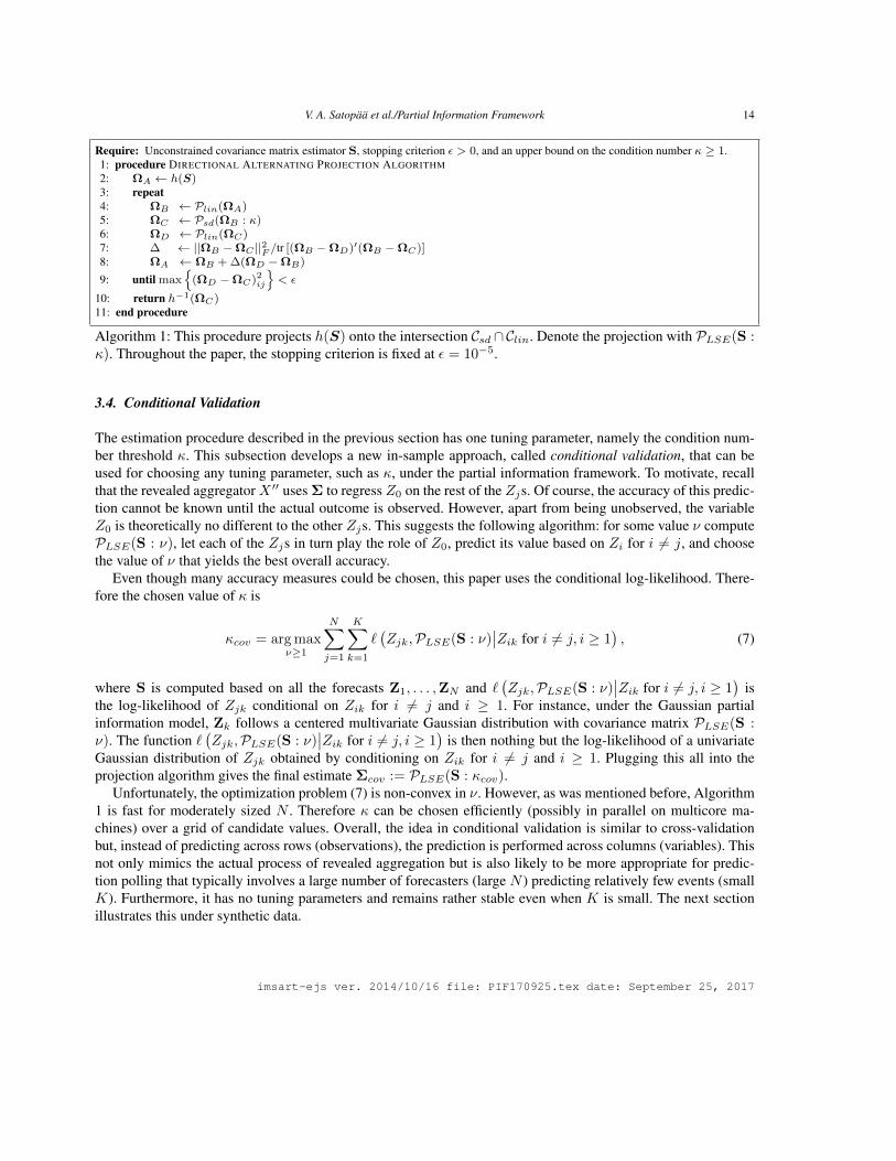
set. The general form of the algorithm does not specify which projection should be called twice. Therefore, giventhat Psd(· : κ) takes longer to run than Plin(·), it is beneficial to choose to call Plin(·) twice. The complexityof each iteration is determined largely by the spectral decomposition which is fairly fast for moderately large N .Overall time to convergence, of course, depends on the choice of the stopping criterion. Many intuitive criteria arepossible. Given that ΩD ∈ Clin and ΩC ∈ Csd, the stopping criterion max(ΩD −ΩC)2ij < ε suggests that thereturn value is in Csd and close to Clin in every direction. Based on our experience, the algorithm converges quitequickly. For instance, our implementation in C++ generally solves (6) for ε = 10−5 and N = 100 in less than asecond on a 1.7 GHz Intel Core i5 computer. This code will be made available online upon publication. For theremainder of the paper, projecting S onto the feasible region is denoted with the operator PLSE(S : κ).
imsart-ejs ver. 2014/10/16 file: PIF170925.tex date: September 25, 2017
V. A. Satopaa et al./Partial Information Framework 14
Require: Unconstrained covariance matrix estimator S, stopping criterion ε > 0, and an upper bound on the condition number κ ≥ 1.1: procedure DIRECTIONAL ALTERNATING PROJECTION ALGORITHM2: ΩA ← h(S)3: repeat4: ΩB ← Plin(ΩA)5: ΩC ← Psd(ΩB : κ)6: ΩD ← Plin(ΩC)7: ∆ ← ||ΩB −ΩC ||2F /tr [(ΩB −ΩD)′(ΩB −ΩC)]8: ΩA ← ΩB + ∆(ΩD −ΩB)
9: until max
(ΩD −ΩC)2ij
< ε
10: return h−1(ΩC)11: end procedure
Algorithm 1: This procedure projects h(S) onto the intersection Csd ∩Clin. Denote the projection with PLSE(S :κ). Throughout the paper, the stopping criterion is fixed at ε = 10−5.
3.4. Conditional Validation
The estimation procedure described in the previous section has one tuning parameter, namely the condition num-ber threshold κ. This subsection develops a new in-sample approach, called conditional validation, that can beused for choosing any tuning parameter, such as κ, under the partial information framework. To motivate, recallthat the revealed aggregatorX ′′ uses Σ to regress Z0 on the rest of the Zjs. Of course, the accuracy of this predic-tion cannot be known until the actual outcome is observed. However, apart from being unobserved, the variableZ0 is theoretically no different to the other Zjs. This suggests the following algorithm: for some value ν computePLSE(S : ν), let each of the Zjs in turn play the role of Z0, predict its value based on Zi for i 6= j, and choosethe value of ν that yields the best overall accuracy.
Even though many accuracy measures could be chosen, this paper uses the conditional log-likelihood. There-fore the chosen value of κ is
κcov = arg maxν≥1
N∑j=1
K∑k=1
`(Zjk,PLSE(S : ν)
∣∣Zik for i 6= j, i ≥ 1), (7)
where S is computed based on all the forecasts Z1, . . . ,ZN and `(Zjk,PLSE(S : ν)
∣∣Zik for i 6= j, i ≥ 1)
isthe log-likelihood of Zjk conditional on Zik for i 6= j and i ≥ 1. For instance, under the Gaussian partialinformation model, Zk follows a centered multivariate Gaussian distribution with covariance matrix PLSE(S :ν). The function `
(Zjk,PLSE(S : ν)
∣∣Zik for i 6= j, i ≥ 1)
is then nothing but the log-likelihood of a univariateGaussian distribution of Zjk obtained by conditioning on Zik for i 6= j and i ≥ 1. Plugging this all into theprojection algorithm gives the final estimate Σcov := PLSE(S : κcov).
Unfortunately, the optimization problem (7) is non-convex in ν. However, as was mentioned before, Algorithm1 is fast for moderately sized N . Therefore κ can be chosen efficiently (possibly in parallel on multicore ma-chines) over a grid of candidate values. Overall, the idea in conditional validation is similar to cross-validationbut, instead of predicting across rows (observations), the prediction is performed across columns (variables). Thisnot only mimics the actual process of revealed aggregation but is also likely to be more appropriate for predic-tion polling that typically involves a large number of forecasters (large N ) predicting relatively few events (smallK). Furthermore, it has no tuning parameters and remains rather stable even when K is small. The next sectionillustrates this under synthetic data.
imsart-ejs ver. 2014/10/16 file: PIF170925.tex date: September 25, 2017

V. A. Satopaa et al./Partial Information Framework 15
5 10 15 20 25 30 35
0.0
0.5
1.0
1.5
2.0
RM
SE
Number of Problems, K
κ = 10
κ = 10000
κ = 1000κ = 100
κcov
(a) Prediction accuracy under fixed N = 20 but differentvalues of K.
5 10 15 20 25 30 350.
00.
20.
40.
60.
81.
0R
MS
E
Number of Forecasters, N
κ = 10
κ = 10000
κ = 1000κ = 100κcov
(b) Prediction accuracy under fixed K = 20 but differentvalues of N .
Fig 3: The accuracy to predict Yk under different values of N and K. Each line represents a different choice of κin X ′′ = diag(Σ)′Σ−1Xk with Σ = PLSE(SX : κ).
4. SYNTHETIC DATA ANALYSIS
This section briefly evaluates different aggregators under synthetic data generated from the multivariate Gaussiandistribution (3). The analysis provides insight into the behavior of the estimation procedure and also introducesthe simplest instance of the Gaussian model.
Model Instance. The link function g(·) is the identity. Thus, the target quantity is Yk = g(Z0k) =Z0k, and the forecasts are Xjk = E(Yk|Zjk) = Zjk for all j and k. The revealed aggregator for eventk is X ′′k = diag(Σ)′Σ−1Xk, where Xk = (X1k, . . . , XNk)′.
Simulating forecasts from (3) requires a Σ such that h(Σ) ∈ SN+1+ . One approach is to draw a N × N
matrix from a Wishart distribution, scale it such that all diagonal entries are within [0, 1], and then accept it asΣ if this implies h(Σ) ∈ SN+1
+ . However, it is easy to show via simulation that the rate at which the randomlygenerated matrix is accepted decreases in N and is very close to zero already for N = 5. Therefore this sectionadopts a different approach that samples Σ with full acceptance rate but only within a subset of all informationstructures: first pick δj
i.i.d.∼ U(0.1, 0.9) and then set ρij = δiδj for all i 6= j. This way Σ− diag(Σ)diag(Σ)′ =Diag((δ1 − δ21 , . . . , δN − δ2N )′) ∈ SN+ , which, by the Schur complement, satisfies h(Σ) ∈ SN+1
+ . Finally, the
outcome and forecasts for the kth event are drawn from (Yk,Xk) = (Z0k, Z1k, . . . , ZNk)′i.i.d.∼ NN+1(0, h(Σ)).
These forecasts are aggregated in the following ways:
1. X ′′S(SX) = diag(SX)′S−1X Xk, where SX is the sample covariance matrix. Given that SX is singular when
imsart-ejs ver. 2014/10/16 file: PIF170925.tex date: September 25, 2017

V. A. Satopaa et al./Partial Information Framework 16
Average Median Xcov'' Xtrue
''
5 10 15 20 25 30 35
0.20
0.25
0.30
0.35
0.40
0.45
0.50
RM
SE
Number of Problems, K
(a) Prediction accuracy under fixed N = 20 but differentvalues of K.
5 10 15 20 25 30 35
0.2
0.3
0.4
0.5
RM
SE
Number of Forecasters, N
(b) Prediction accuracy under fixed K = 20 but differentvalues of N .
Fig 4: The accuracy to predict Yk under different values of N and K. The aggregator X ′′true assumes knowledgeof the true information structure and hence represents optimal accuracy.
K < N , its inverse is computed with the generalized inverse.2. X ′′ = diag(Σ)′Σ−1Xk for Σ = PLSE(SX : κ) and fixed κ = 10, 100, 1000, or 10000.3. X ′′cov = diag(Σcov)
′Σ−1covXk with Σcov = PLSE(SX : κcov). The condition number constraint κcov isfound over a grid of 100 values between 10 and 1000.
4. X ′′true = diag(Σ)′Σ−1Xk. This aggregator assumes the knowledge of the true Σ and hence representsoptimal performance.
5. The average forecast6. The median forecast
The overall process is repeated 5, 000 times under different values of K and N , each ranging from 5 to 35 withconstant increments of 5. Performance is then measured with the average root-mean-squared-error (RMSE) inpredicting Yk across all 5, 000 iterations.
To begin, Figure 3 compares the average RMSEs of X ′′ = diag(Σ)′Σ−1Xk with Σ = PLSE(SX : κ) andfixed κ = 10, 100, 1000, or 10000 against the average RMSE of X ′′cov . Figure 3a varies K but fixes N = 20.Figure 3b, on the other hand, varies N but fixes K = 20. Overall, X ′′cov achieves the lowest RMSE in all casesexcept when N = 5 and K = 20. Thus, even though the performance of X ′′ is clearly sensitive to the value of κ,a good choice can be found with the conditional validation procedure described in Section 3.4.
imsart-ejs ver. 2014/10/16 file: PIF170925.tex date: September 25, 2017

V. A. Satopaa et al./Partial Information Framework 17
Figure 4 shows the average RMSEs of the competing aggregators enumerated above. Similarly to Figure 3,either N or K is held fixed while the other varies. Given that Yk = Z0k ∼ N (0, 1), the RMSE of the priormean E(
√(Yk − 0)2) = E(|Yk|) =
√2/π ≈ 0.8 can be considered as the upper bound in prediction error. The
lower bound, on the other hand, is given by X ′′true. The revealed aggregator X ′′S typically received a loss muchlarger than 0.8 and is therefore not included in the figure. Overall, the two measurement-error aggregators, namelyaverage and median perform very similarly, with RMSE around 0.5. They both show slight improvement as Nincreases. In all cases, however, their RMSE is uniformly well above that of X ′′true and X ′′cov , suggesting thatmeasurement-error aggregators are a poor choice when forecasts truly arise from a partial information model. Therevealed aggregator X ′′cov collects information and appears to improve at the optimal rate as N increases. This canbe seen in the way the performance gap from Xtrue to X ′′cov remains approximately constant in Figure 4b. As Kgrows larger, however, X ′′cov approaches X ′′true.
5. APPLICATIONS
This section applies the partial information framework to different types of real world forecasts. For each typethere may be different ways to adopt the Gaussian model. The main point, however, is not to find the optimal wayto do this but rather to illustrate the framework and show how partial information aggregators can outperform thecommon measurement error aggregators.
5.1. Probability Forecasts of Binary Outcomes
5.1.1. Dataset
During the second year of the Good Judgment Project (GJP) the forecasters made probability estimates for 78events, each with two possible outcomes. One of these events was illustrated in Figure 1. Each prediction problemhad a timeframe, defined as the number of days between the first day of forecasting and the anticipated resolutionday. These timeframes varied largely among problems, ranging from 12 days to 519 days with a mean of 185.4days. During each timeframe the forecasters were allowed to update their predictions as frequently as they liked.The forecasters knew that their estimates would be assessed for accuracy using the quadratic loss (often knownas the Brier score; see Brier 1950 for more details). This is a proper loss function that incentivized the forecastersto report their true beliefs instead of attempting to game the system. In addition to receiving $150 for meetingminimum participation requirements that did not depend on prediction accuracy, the forecasters received statusrewards for their performance via leader-boards displaying the losses for the best 20 forecasters. Depending on thedetails of the reward structure, such a competition for rank may eliminate the truth-revelation property of properloss functions (see, e.g., Lichtendahl Jr and Winkler 2007).
This data collection raises several issues. First, given that the current paper does not focus on modeling dynamicdata, only forecasts made within some common time interval should be considered. Second, not all forecastersmade predictions for all the events. Furthermore, the forecasters generally updated their forecasts infrequently, re-sulting into a very sparse dataset. To somewhat alleviate the effect of missing values, only the hundred most activeforecasters are considered. This makes sufficient overlap highly likely but, unfortunately, still not guaranteed.
All these considerations lead to a parallel analysis of three scenarios: High Uncertainty (HU), Medium Un-certainty (MU), and Low Uncertainty (LU). Important differences are summarized in Table 1. Each scenarioconsiders the forecasters’ most recent prediction within a different time interval. For instance, LU only includeseach forecaster’s most recent forecast during 30 − 60 days before the anticipated resolution day. The resultingdataset has 60 events of which 13 occurred. In the corresponding 60× 100 table of forecasts, around 42 % of thevalues are missing. The other two scenarios are defined similarly.
imsart-ejs ver. 2014/10/16 file: PIF170925.tex date: September 25, 2017
V. A. Satopaa et al./Partial Information Framework 18
TABLE 1Summary of the three time intervals analyzed. Each scenario considers the forecasters’ most recent forecasts within the given time interval.
The value in the parentheses represent the number of events occurred. The final column shows the percent of missing forecasts.
Scenario Time Interval # of Events Missing (%)High Uncertainty (HU) 90− 120 49 (10) 51Medium Uncertainty (MU) 60− 90 56 (14) 46Low Uncertainty (LU) 30− 60 60 (13) 42
5.1.2. Model Specification and Aggregation
The first step is to pick a link function and derive a Gaussian model for probability forecasts of binary events.Overall, this construction resembles in many ways the latent variable version of a standard probit model.
Model Instance. Identify the kth event with Yk ∈ 0, 1. These outcomes link to the informationvariables via the following function:
Yk = g(Z0k) =
1 if Z0k > tk
0 otherwise,
where tk ∈ R is some threshold value. Therefore the link function g(·) is simply the indicator function1Ak
of the event Ak = Z0k > tk. This threshold is defined by the prior probability of the kth eventP(Yk = 1) = Φ(−tk), where Φ(·) is the CDF of a standard Gaussian distribution. Given that thethresholds are allowed to vary among the events, each event has its own prior. The correspondingprobability forecasts Xjk ∈ [0, 1] are
Xjk = E(Yk|Zjk) = Φ
(Zjk − tk√
1− δj
).
In a similar manner, the revealed aggregator X ′′k ∈ [0, 1] for event k is
X ′′k = E(Yk|Zk) = Φ
(diag(Σ)′Σ−1Zk − tk√
1− diag(Σ)′Σ−1diag(Σ)
). (8)
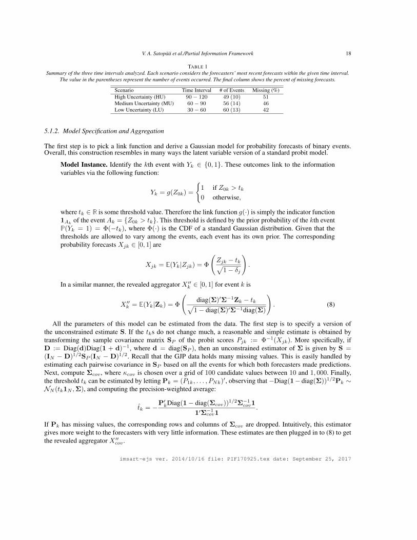
All the parameters of this model can be estimated from the data. The first step is to specify a version ofthe unconstrained estimate S. If the tks do not change much, a reasonable and simple estimate is obtained bytransforming the sample covariance matrix SP of the probit scores Pjk := Φ−1(Xjk). More specifically, ifD := Diag(d)Diag(1 + d)−1, where d = diag(SP ), then an unconstrained estimator of Σ is given by S =(IN − D)1/2SP (IN − D)1/2. Recall that the GJP data holds many missing values. This is easily handled byestimating each pairwise covariance in SP based on all the events for which both forecasters made predictions.Next, compute Σcov , where κcov is chosen over a grid of 100 candidate values between 10 and 1, 000. Finally,the threshold tk can be estimated by letting Pk = (P1k, . . . , PNk)′, observing that −Diag(1− diag(Σ))1/2Pk ∼NN (tk1N ,Σ), and computing the precision-weighted average:
tk = −P′kDiag(1− diag(Σcov))1/2Σ−1cov1
1′Σ−1cov1.
If Pk has missing values, the corresponding rows and columns of Σcov are dropped. Intuitively, this estimatorgives more weight to the forecasters with very little information. These estimates are then plugged in to (8) to getthe revealed aggregator X ′′cov .
imsart-ejs ver. 2014/10/16 file: PIF170925.tex date: September 25, 2017
V. A. Satopaa et al./Partial Information Framework 19
Average Median Log−odds Probit Xcov''
10 20 30 40 50 60
0.27
0.28
0.29
0.30
0.31
0.32
RM
SE
Number of Forecasters, N
(a) High Uncertainty (HU)
10 20 30 40 50 60
0.20
0.22
0.24
0.26
0.28
RM
SE
Number of Forecasters, N
(b) Medium Uncertainty (MU)
10 20 30 40 50 60
0.16
0.18
0.20
0.22
0.24
RM
SE
Number of Forecasters, N
(c) Low Uncertainty (LU)
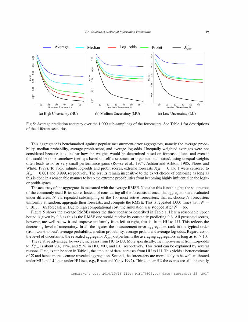
Fig 5: Average prediction accuracy over the 1,000 sub-samplings of the forecasters. See Table 1 for descriptionsof the different scenarios.
This aggregator is benchmarked against popular measurement-error aggregators, namely the average proba-bility, median probability, average probit-score, and average log-odds. Unequally weighted averages were notconsidered because it is unclear how the weights would be determined based on forecasts alone, and even ifthis could be done somehow (perhaps based on self-assessment or organizational status), using unequal weightsoften leads to no or very small performance gains (Rowse et al., 1974; Ashton and Ashton, 1985; Flores andWhite, 1989). To avoid infinite log-odds and probit scores, extreme forecasts Xjk = 0 and 1 were censored toXjk = 0.001 and 0.999, respectively. The results remain insensitive to the exact choice of censoring as long asthis is done in a reasonable manner to keep the extreme probabilities from becoming highly influential in the logit-or probit-space.
The accuracy of the aggregates is measured with the average RMSE. Note that this is nothing but the square rootof the commonly used Brier score. Instead of considering all the forecasts at once, the aggregators are evaluatedunder different N via repeated subsampling of the 100 most active forecasters; that is, choose N forecastersuniformly at random, aggregate their forecasts, and compute the RMSE. This is repeated 1,000 times with N =5, 10, . . . , 65 forecasters. Due to high computational cost, the simulation was stopped after N = 65.
Figure 5 shows the average RMSEs under the three scenarios described in Table 1. Here a reasonable upperbound is given by 0.5 as this is the RMSE one would receive by constantly predicting 0.5. All presented scores,however, are well below it and improve uniformly from left to right, that is, from HU to LU. This reflects thedecreasing level of uncertainty. In all the figures the measurement-error aggregators rank in the typical order(from worst to best): average probability, median probability, average probit, and average log-odds. Regardless ofthe level of uncertainty, the revealed aggregator X ′′cov outperforms the averaging aggregators as long as K ≥ 10.
The relative advantage, however, increases from HU to LU. More specifically, the improvement from Log-oddsto X ′′cov is about 2%, 17%, and 21% in HU, MU, and LU, respectively. This trend can be explained by severalreasons. First, as can be seen in Table 1, the amount of data increases from HU to LU. This yields a better estimateof Σ and hence more accurate revealed aggregation. Second, the forecasters are more likely to be well-calibratedunder MU and LU than under HU (see, e.g., Braun and Yaniv 1992). Third, under HU the events are still inherently
imsart-ejs ver. 2014/10/16 file: PIF170925.tex date: September 25, 2017

V. A. Satopaa et al./Partial Information Framework 20
very uncertain. Consequently, the forecasters are unlikely to hold much useful information as a group. Instead,forecast variation is likely to be dominated by noise. In such settings measurement-error aggregators generallyperform relatively well (Satopaa et al. 2016). In the contrary, under MU the events have lost a part of their inherentuncertainty, allowing some forecasters to possess useful private information. These individuals are then prioritizedby X ′′cov while the averaging-aggregators continue to treat all forecasts equally. Consequently, the performance ofthe measurement error aggregators plateaus after N = 30 or so. Therefore having more than about 30 forecastersdoes not make a large difference if one is determined to aggregate their predictions using the measurement errortechniques; a similar results was reported by Satopaa et al. (2014a). In contrast, however, the RMSE of X ′′covcontinues to improve almost linearly in N , suggesting that X ′′cov is able to find some residual information in eachadditional forecaster and use this to increase its performance advantage.
5.1.3. Information Diversity
The GJP assigned the forecasters to make predictions either in isolation or in teams. Furthermore, after the firstyear of the tournament, the top 2% forecasters were elected to the elite group of “super-forecasters.” These super-forecasters then worked in exclusive teams to make highly accurate predictions on the same events as the rest of theforecasters. Overall, these assignments directly suggest a level of information overlap. In particular, recalling theinterpretation of Σ from Section 2.2.1, super-forecasters can be expected to have the highest δjs and forecastersin the same team should have a relatively high ρij . This subsection shows that Σcov aligns well with this priorknowledge about the forecasters’ information structure.
For the sake of brevity, only the LU scenario is analyzed as this is where X ′′cov presented the highest rela-tive improvement. The associated 100 forecasters involve 36 individuals predicting in isolation, 33 forecastingteam-members (across 24 teams), and 31 super-forecasters (across 5 teams). Figure 6a displays Σcov for the fivemost active forecasters. This group involves two forecasters working in isolation (Iso. A and B) and three super-forecasters (Sup. A, B, and C), of whom the super-forecasters A and B are in the same team. Overall, Σcov agreeswith this classification: the only two team members, namely Sup. A and B have a relatively high informationoverlap. In addition, the three super-forecasters are more informed than the non-super-forecasters. Such a highlevel of information unavoidably leads to higher information overlap with the rest of the forecasters.
By and large, this agreement generalizes to the entire group of forecasters. To illustrate, Figure 6b displaysΣcov for all the 100 forecasters. The information structure has been ordered with respect to the diagonal such thatthe more informed forecasters appear on the right. Furthermore, a colored rug has been appended on the top. Thisrug shows whether each forecaster worked in isolation, in a non-super-forecaster team, or in a super-forecasterteam. These results agree with our prior knowledge: the super-forecasters are mostly situated on the right amongthe most informed forecasters. The average estimated δj among the super-forecaster is 0.80. On the other hand,the average estimated δj among the individuals working in isolation or in non-super-forecaster teams are 0.47and 0.50, respectively. Therefore working in a team makes the forecasters’ predictions, on average, slightly moreinformed.
5.2. Point Forecasts of Continuous Outcomes
5.2.1. Dataset
Moore and Klein (2008) hired 415 undergraduates from Carnegie Mellon University to guess the weights of 20people based on a series of pictures. These forecasts were illustrated in Figure 2. The target people were between7 and 62 years old and had weights ranging from 61 to 230 pounds, with a mean of 157.6 pounds. All the students
imsart-ejs ver. 2014/10/16 file: PIF170925.tex date: September 25, 2017

V. A. Satopaa et al./Partial Information Framework 21
Iso. A Iso. B Sup. A Sup. B Sup. C
0.4
0.5
0.6
0.7
0.8
(a) Σcov for the five most active forecasters
Isolation Team Super
0.0
0.2
0.4
0.6
0.8
(b) Σcov for all 100 forecasters shows high information diver-sity.
Fig 6: The estimated information structure Σ under the LU scenario. Each forecaster worked either in isolation, ina non-super-forecaster team, or in a super-forecaster team. The super-forecasters generally have more informationthan the forecasters working in isolation.
were shown the same pictures and hence given the exact same information. Therefore any information diversityarises purely from the participants’ decisions to use different subsets of the same information. Consequently, theleast and most informed forecasters are likely to more similar than in Section 5.1, where diversity also stemmedfrom differences in the information available to the forecasters.
Unlike in Section 5.1, the Gaussian model can be applied almost directly to the data. Only the effect of extremevalues was reduced via a 90% Winsorization (Hastings et al., 1947). This handled some obvious outliers. Forinstance, the original dataset contained a few estimates above 1000 pounds and as low as 10 pounds. Winsorizationgenerally improved the performance of all the competing aggregators.
imsart-ejs ver. 2014/10/16 file: PIF170925.tex date: September 25, 2017

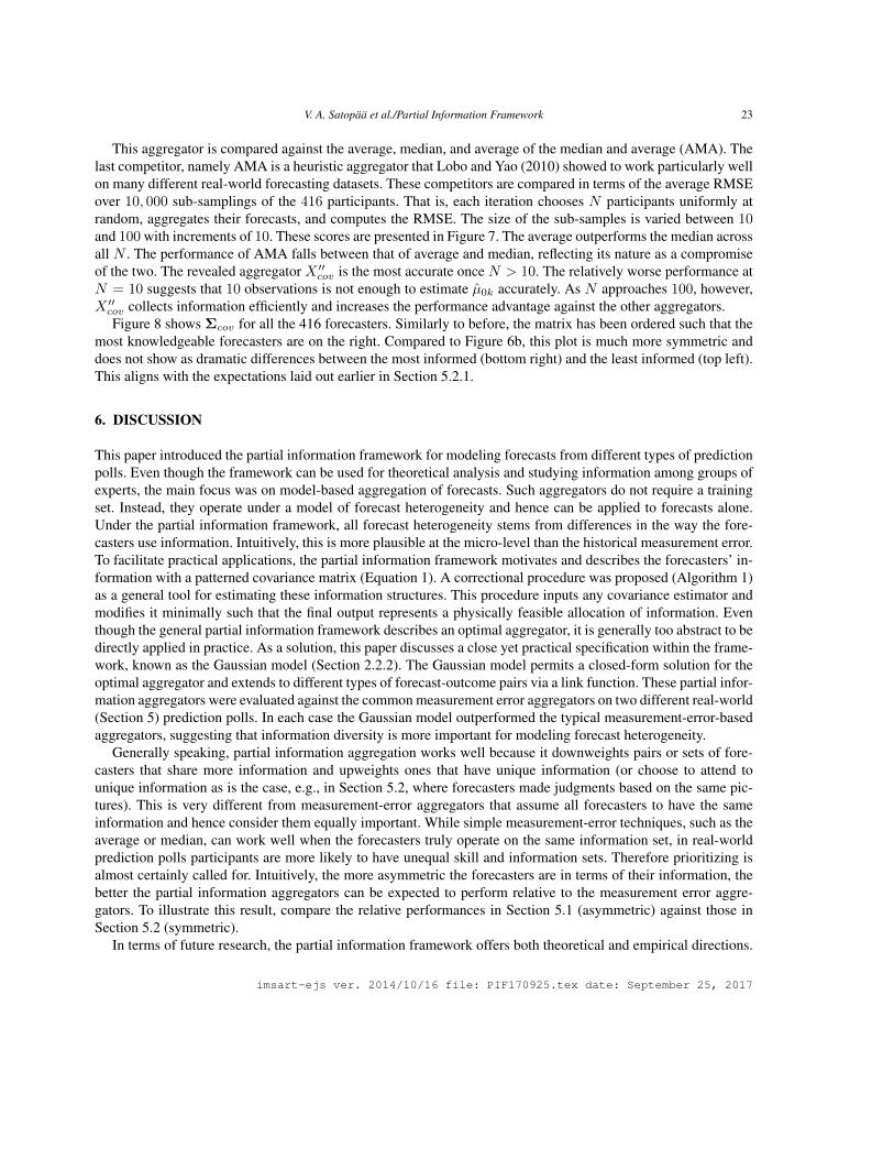
V. A. Satopaa et al./Partial Information Framework 22
AverageMedian
AMAXcov
''
20 40 60 80 10020.4
20.6
20.8
21.0
21.2
21.4
RM
SE
Number of Forecasters, N
Fig 7: Average prediction accuracy Fig 8: Σcov for all 416 forecasters shows low informa-tion diversity.
5.2.2. Model Specification and Aggregation
Model Instance. Suppose Yk andXjk are real-valued. If the proper non-informative prior distributionof Yk isN (µ0k, σ
20), then Yk = g(Z0k) = Z0kσ0 +µ0k. Consequently,Xjk = E(Y |Zjk) = Zjkσ0 +
µ0k for all j = 1, . . . , N . Therefore Xj ∼ N (µ0k, σ2j ) for some σ2
j ≤ σ20 . If Zk = (Z1k, . . . , ZNk)
′,then the revealed aggregator for the kth event is
X ′′k = E (Yk|Zk) = diag(Σ)′Σ−1Zkσ0 + µ0k. (9)
Under this model the prior distribution of Yk is specified by µ0k and σ20 . Given that E(Xjk) = µ0k for all
j = 1, . . . , N , the sample average µ0k =∑Nj=1Xjk/N provides an initial estimate of µ0k. The value of σ2
0 can beestimated by assuming a distribution for the σ2
j s. More specifically, let σ2j be i.i.d. on the interval [0, σ2
0 ] and use the
resulting likelihood to estimate σ20 . For instance, a non-informative choice is to assume σ2
ji.i.d.∼ U(0, σ2
0), whichleads to the maximum likelihood estimator maxσ2
j . This has a downward bias that can be corrected by a multi-plicative factor of (N+1)/N . Therefore, replacing σ2
j with the sample variance sj =∑Kk=1(Xjk−µ0k)2/(K−1)
gives the final estimate σ20 = (N + 1)/N maxsj. Using these estimates, the Xjks can be transformed into the
Zjks whose sample covariance matrix SZ provides the unconstrained estimator for the projection algorithm. Thevalue of κcov is chosen over a grid of 10 values between 10 and 10, 000. Once Σcov has been computed, the priormeans are updated with the precision-weighted averages µ0k = (X′kΣ
−1cov1N )/(1′NΣ−1cov1N ). In the end, all these
estimates are plugged in (9) to get the revealed aggregator X ′′cov .
imsart-ejs ver. 2014/10/16 file: PIF170925.tex date: September 25, 2017
V. A. Satopaa et al./Partial Information Framework 23
This aggregator is compared against the average, median, and average of the median and average (AMA). Thelast competitor, namely AMA is a heuristic aggregator that Lobo and Yao (2010) showed to work particularly wellon many different real-world forecasting datasets. These competitors are compared in terms of the average RMSEover 10, 000 sub-samplings of the 416 participants. That is, each iteration chooses N participants uniformly atrandom, aggregates their forecasts, and computes the RMSE. The size of the sub-samples is varied between 10and 100 with increments of 10. These scores are presented in Figure 7. The average outperforms the median acrossall N . The performance of AMA falls between that of average and median, reflecting its nature as a compromiseof the two. The revealed aggregator X ′′cov is the most accurate once N > 10. The relatively worse performance atN = 10 suggests that 10 observations is not enough to estimate µ0k accurately. As N approaches 100, however,X ′′cov collects information efficiently and increases the performance advantage against the other aggregators.
Figure 8 shows Σcov for all the 416 forecasters. Similarly to before, the matrix has been ordered such that themost knowledgeable forecasters are on the right. Compared to Figure 6b, this plot is much more symmetric anddoes not show as dramatic differences between the most informed (bottom right) and the least informed (top left).This aligns with the expectations laid out earlier in Section 5.2.1.
6. DISCUSSION
This paper introduced the partial information framework for modeling forecasts from different types of predictionpolls. Even though the framework can be used for theoretical analysis and studying information among groups ofexperts, the main focus was on model-based aggregation of forecasts. Such aggregators do not require a trainingset. Instead, they operate under a model of forecast heterogeneity and hence can be applied to forecasts alone.Under the partial information framework, all forecast heterogeneity stems from differences in the way the fore-casters use information. Intuitively, this is more plausible at the micro-level than the historical measurement error.To facilitate practical applications, the partial information framework motivates and describes the forecasters’ in-formation with a patterned covariance matrix (Equation 1). A correctional procedure was proposed (Algorithm 1)as a general tool for estimating these information structures. This procedure inputs any covariance estimator andmodifies it minimally such that the final output represents a physically feasible allocation of information. Eventhough the general partial information framework describes an optimal aggregator, it is generally too abstract to bedirectly applied in practice. As a solution, this paper discusses a close yet practical specification within the frame-work, known as the Gaussian model (Section 2.2.2). The Gaussian model permits a closed-form solution for theoptimal aggregator and extends to different types of forecast-outcome pairs via a link function. These partial infor-mation aggregators were evaluated against the common measurement error aggregators on two different real-world(Section 5) prediction polls. In each case the Gaussian model outperformed the typical measurement-error-basedaggregators, suggesting that information diversity is more important for modeling forecast heterogeneity.
Generally speaking, partial information aggregation works well because it downweights pairs or sets of fore-casters that share more information and upweights ones that have unique information (or choose to attend tounique information as is the case, e.g., in Section 5.2, where forecasters made judgments based on the same pic-tures). This is very different from measurement-error aggregators that assume all forecasters to have the sameinformation and hence consider them equally important. While simple measurement-error techniques, such as theaverage or median, can work well when the forecasters truly operate on the same information set, in real-worldprediction polls participants are more likely to have unequal skill and information sets. Therefore prioritizing isalmost certainly called for. Intuitively, the more asymmetric the forecasters are in terms of their information, thebetter the partial information aggregators can be expected to perform relative to the measurement error aggre-gators. To illustrate this result, compare the relative performances in Section 5.1 (asymmetric) against those inSection 5.2 (symmetric).
In terms of future research, the partial information framework offers both theoretical and empirical directions.
imsart-ejs ver. 2014/10/16 file: PIF170925.tex date: September 25, 2017

V. A. Satopaa et al./Partial Information Framework 24
Require: Condition number threshold κ ≥ 1 and sample eigenvalues in ascending order l1 ≤ l2 ≤ · · · ≤ lN+1.1: procedure BINARY-SEARCH OPTIMIZATION2: Initialize D ← maxl1, 0 and U ← lN+1/κ.3: µ0 ← (D + U)/24: for n = 0, 1, . . . do5: Compute µ∗n, dn, and un.6: if µ∗n < 0 and dn < 0 then7: return 08: else if µ∗n < dn then9: U ← dn
10: else if µ∗n > un then11: D ← un12: else13: return µ∗n14: end if15: µn+1 ← (D + U)/216: end for17: return µ∗n18: end procedure
Algorithm 2: This procedure solves (10) efficiently using the structure of the problem and binary-search.
One theoretical avenue involves estimation of information overlap. In some cases the higher order overlaps havebeen found to be irrelevant to aggregation. For instance, DeGroot and Mortera (1991) show that the pairwiseconditional (on the truth) distributions of the forecasts are sufficient for computing the optimal weights of aweighted average. Theoretical results on the significance or insignificance of higher order overlaps under thepartial information framework would be desirable. Given that the Gaussian model can only accommodate pairwiseinformation overlap, such a result would reveal the need of a specification that is more complex than the Gaussianmodel.
A promising empirical direction is the Bayesian approach. These techniques are very natural for fitting hierar-chical models such as the ones discussed in this paper. Furthermore, in many applications with small or moderatelysized datasets, Bayesian methods have been found to be more stable than the likelihood-based alternatives. There-fore, given that the number of forecasts in a prediction poll is typically quite small, a Bayesian approach is likelyto improve the quality of the final aggregate. This would involve developing a prior distribution for the informa-tion structure – a problem that seems interesting in itself. Overall, this avenue should certainly be pursued, andthe results tested against other high performing aggregators.
Appendix A: Finding µ∗ for Psd(· : κ)
This section describes a binary-search-like algorithm to solve
µ∗ = arg minµ≥0
π(µ) = arg minµ≥0
N∑i=1
((µ− li)2+ + (li − κµ)
2+
). (10)
First, it can be assumed that cond(h(SZ)) /∈ [1, κ]; otherwise, the projection can simply return h(SZ). Second,max0, l1 ≤ µ ≤ lN+1/κ because otherwise moving µ closer to the nearest sample eigenvalue decreases π(µ).Now, consider some value µn ≥ 0 and two index sets Dn = i : li ≤ µn and Un = i : µnκ ≤ li. Then,
π(µn) =∑i∈Dn
(µn − li)2 +∑i∈Un
(li − κµn)2,
imsart-ejs ver. 2014/10/16 file: PIF170925.tex date: September 25, 2017

V. A. Satopaa et al./Partial Information Framework 25
which has a global minimum at
µ∗n =
∑i∈Dn
li + κ∑i∈Un
li
|Dn|+ κ2|Un|.
The operator |A| denotes the number of elements in the set A. Let dn and un denote the minimum and maximum,respectively, of the interval where any value of µ gives the index sets Dn and Un. To make this specific, definetwo operators:
d(µ) = maxli : li ≤ µ and u(µ) = minli : li ≥ µ.
If no value is found, then d(µ) = 0 and u(µ) = +∞. Then,
dn = maxd(µn), d(µnκ)/κ and un = minu(µn), u(µnκ)/κ.
Of course, µ∗n is the solution to (10) as long as µ∗n ∈ (dn, un]. If, on the other hand, µ∗n is less than dn (or greaterthan un), the global minimum µ∗ must be smaller than dn (or greater than un). If µ∗n is, say, less than dn, then anatural approach is to update µn to µn+1 that is somewhere between dn and some known lower bound of µ. Thisgives rise to a binary-search-like algorithm described in Algorithm 2.
ACKNOWLEDGEMENTS
The authors would like to thank Don Moore for providing us with the weight dataset.
REFERENCES
Ashton, A. H. and Ashton, R. H. (1985). Aggregating subjective forecasts: Some empirical results. ManagementScience, 31(12):1499–1508.
Banerjee, A., Guo, X., and Wang, H. (2005). On the optimality of conditional expectation as a bregman predictor.Information Theory, IEEE Transactions on, 51(7):2664–2669.
Braun, P. A. and Yaniv, I. (1992). A case study of expert judgment: Economists’ probabilities versus base-ratemodel forecasts. Journal of Behavioral Decision Making, 5(3):217–231.
Breiman, L. (1996). Stacked regressions. Machine Learning, 24(1):49–64.Brier, G. W. (1950). Verification of forecasts expressed in terms of probability. Monthly Weather Review, 78:1–3.Broecker, J. (2012). Forecast verification: a practitioner’s guide in atmospheric science, chapter 7.2.2, pages
121–122. John Wiley & Sons, Chichester, UK, 2nd edition.Daniels, M. J. and Kass, R. E. (2001). Shrinkage estimators for covariance matrices. Biometrics, 57(4):1173–
1184.Dawid, A., DeGroot, M., Mortera, J., Cooke, R., French, S., Genest, C., Schervish, M., Lindley, D., McConway,
K., and Winkler, R. (1995). Coherent combination of experts’ opinions. TEST, 4(2):263–313.Dawid, A. P. (1982). The well-calibrated bayesian. Journal of the American Statistical Association, 77(379):605–
610.DeGroot, M. H. and Mortera, J. (1991). Optimal linear opinion pools. Management Science, 37(5):546–558.Di Bacco, M., Frederic, P., and Lad, F. (2003). Learning from the probability assertions of experts. Research
Report. Available at: http://www.math.canterbury.ac.nz/research/ucdms2003n6.pdf.Dowie, J. (1976). On the efficiency and equity of betting markets. Economica, 43(170):139–150.
imsart-ejs ver. 2014/10/16 file: PIF170925.tex date: September 25, 2017

V. A. Satopaa et al./Partial Information Framework 26
Flores, B. E. and White, E. M. (1989). Subjective versus objective combining of forecasts: an experiment. Journalof Forecasting, 8(3):331–341.
Foster, D. P. and Vohra, R. V. (1998). Asymptotic calibration. Biometrika, 85(2):379–390.Gigerenzer, G., Hoffrage, U., and Kleinbolting, H. (1991). Probabilistic mental models: a brunswikian theory of
confidence. Psychological Review, 98(4):506.Gneiting, T., Ranjan, R., et al. (2013). Combining predictive distributions. Electronic Journal of Statistics,
7:1747–1782.Goel, S., Reeves, D. M., Watts, D. J., and Pennock, D. M. (2010). Prediction without markets. In Proceedings of
the 11th ACM conference on Electronic commerce, pages 357–366. ACM.Gubin, L., Polyak, B., and Raik, E. (1967). The method of projections for finding the common point of convex
sets. USSR Computational Mathematics and Mathematical Physics, 7(6):1–24.Hastings, C., Mosteller, F., Tukey, J. W., and Winsor, C. P. (1947). Low moments for small samples: A comparative
study of order statistics. The Annals of Mathematical Statistics, 18(3):413–426.Hong, L. and Page, S. (2009). Interpreted and generated signals. Journal of Economic Theory, 144(5):2174–2196.Hwang, S.-G. (2004). Cauchy’s interlace theorem for eigenvalues of hermitian matrices. American Mathematical
Monthly, 111:157–159.Johnson, R. A., Wichern, D. W., et al. (2014). Applied multivariate statistical analysis, volume 4. Prentice-Hall
New Jersey.Juslin, P. (1993). An explanation of the hard-easy effect in studies of realism of confidence in one’s general
knowledge. European Journal of Cognitive Psychology, 5(1):55–71.Keren, G. (1987). Facing uncertainty in the game of bridge: A calibration study. Organizational Behavior and
Human Decision Processes, 39(1):98–114.Ladha, K. K. (1992). The condorcet jury theorem, free speech, and correlated votes. American Journal of Political
Science, pages 617–634.Langford, E., Schwertman, N., and Owens, M. (2001). Is the property of being positively correlated transitive?
The American Statistician, 55(4):322–325.Lichtendahl Jr, K. C. and Winkler, R. L. (2007). Probability elicitation, scoring rules, and competition among
forecasters. Management Science, 53(11):1745–1755.Lobo, M. S. and Yao, D. (2010). Human judgement is heavy tailed: Empirical evidence and implications for
the aggregation of estimates and forecasts. Available at http://sousalobo.com/researchfiles/Lobo_Yao_MS_11.pdf. (Working paper).
McCullagh, P. and Nelder, J. A. (1989). Generalized linear models, volume 37. CRC press, 2nd edition.Mellers, B., Ungar, L., Baron, J., Ramos, J., Gurcay, B., Fincher, K., Scott, S. E., Moore, D., Atanasov, P., Swift,
S. A., Murray, T., Stone, E., and Tetlock, P. E. (2014). Psychological strategies for winning a geopoliticalforecasting tournament. Psychological Science, 25(5):1106–1115.
Moore, D. A. and Klein, W. M. (2008). Use of absolute and comparative performance feedback in absolute andcomparative judgments and decisions. Organizational Behavior and Human Decision Processes, 107(1):60–74.
Morris, S. (1995). The common prior assumption in economic theory. Economics & Philosophy, 11(2):227–253.Murphy, A. H. and Daan, H. (1984). Impacts of feedback and experience on the quality of subjective probability
forecasts. comparison of results from the first and second years of the zierikzee experiment. Monthly WeatherReview, 112(3):413–423.
Murphy, A. H. and Winkler, R. L. (1977a). Can weather forecasters formulate reliable probability forecasts ofprecipitation and temperature. National Weather Digest, 2(2):2–9.
Murphy, A. H. and Winkler, R. L. (1977b). Reliability of subjective probability forecasts of precipitation andtemperature. Applied Statistics, 26(1):41–47.
Murphy, A. H. and Winkler, R. L. (1987). A general framework for forecast verification. Monthly Weather Review,
imsart-ejs ver. 2014/10/16 file: PIF170925.tex date: September 25, 2017

V. A. Satopaa et al./Partial Information Framework 27
115(7):1330–1338.Patton, A. J. and Timmermann, A. (2012). Forecast rationality tests based on multi-horizon bounds. Journal of
Business & Economic Statistics, 30(1):1–17.Raftery, A. E., Madigan, D., and Hoeting, J. A. (1997). Bayesian model averaging for linear regression models.
Journal of the American Statistical Association, 92(437):179–191.Ranjan, R. and Gneiting, T. (2010). Combining probability forecasts. Journal of the Royal Statistical Society:
Series B (Statistical Methodology), 72(1):71–91.Ravishanker, N. and Dey, D. K. (2001). A first course in linear model theory. CRC Press.Rowse, G. L., Gustafson, D. H., and Ludke, R. L. (1974). Comparison of rules for aggregating subjective likeli-
hood ratios. Organizational Behavior and Human Performance, 12(2):274–285.Satopaa, V. A. (2017). Combining information from multiple forecasters: General inefficiency of the means.
arXiv:1706.06006.Satopaa, V. A., Baron, J., Foster, D. P., Mellers, B. A., Tetlock, P. E., and Ungar, L. H. (2014a). Combining
multiple probability predictions using a simple logit model. International Journal of Forecasting, 30(2):344–356.
Satopaa, V. A., Jensen, S. T., Mellers, B. A., Tetlock, P. E., Ungar, L. H., et al. (2014b). Probability aggrega-tion in time-series: Dynamic hierarchical modeling of sparse expert beliefs. The Annals of Applied Statistics,8(2):1256–1280.
Satopaa, V. A., Pemantle, R., and Ungar, L. H. (2016). Modeling probability forecasts via information diversity.Journal of the American Statistical Association, 111(516):1623–1633.
Savage, L. J. (1971). Elicitation of personal probabilities and expectations. Journal of the American StatisticalAssociation, 66(336):783–801.
Tanaka, M. and Nakata, K. (2014). Positive definite matrix approximation with condition number constraint.Optimization Letters, 8(3):939–947.
Ungar, L., Mellers, B., Satopaa, V., Tetlock, P., and Baron, J. (2012). The good judgment project: A large scaletest of different methods of combining expert predictions. The Association for the Advancement of ArtificialIntelligence Technical Report FS-12-06.
Won, J. H. and Kim, S.-J. (2006). Maximum likelihood covariance estimation with a condition number constraint.In Signals, Systems and Computers, 2006. ACSSC’06. Fortieth Asilomar Conference on, pages 1445–1449.IEEE.
imsart-ejs ver. 2014/10/16 file: PIF170925.tex date: September 25, 2017