www.business.unsw.edu.au

School of Economics Australian School of Business

UNSW Sydney NSW 2052 Australia

http://www.economics.unsw.edu.au

ISSN 1323-8949

ISBN 978 0 7334 2646 9

Partial Likelihood-Based Scoring Rules for

Evaluating Density Forecasts in Tails

Cees Diks, Valentyn Panchenko

and Dick van Dijk

School of Economics Discussion Paper: 2008/10

The views expressed in this paper are those of the authors and do not necessarily reflect those of the School of Economic at UNSW.

Partial Likelihood-Based Scoring Rules forEvaluating Density Forecasts in Tails∗

Cees Diks†

CeNDEF, Amsterdam School of EconomicsUniversity of Amsterdam

Valentyn Panchenko‡

School of EconomicsUniversity of New South Wales

Dick van Dijk§

Econometric InstituteErasmus University Rotterdam

May 19, 2008

Abstract

We propose new scoring rules based on partial likelihood for assessing the relativeout-of-sample predictive accuracy of competing density forecasts over a specific re-gion of interest, such as the left tail in financial risk management. By construction,existing scoring rules based on weighted likelihood or censored normal likelihoodfavor density forecasts with more probability mass in the given region, renderingpredictive accuracy tests biased towards such densities. Our novel partial likelihood-based scoring rules do not suffer from this problem, as illustrated by means of MonteCarlo simulations and an empirical application to daily S&P 500 index returns.

Keywords: density forecast evaluation; scoring rules; weighted likelihood ratio scores;partial likelihood; risk management.

JEL Classification: C12; C22; C52; C53

∗We would like to thank participants at the 16th Society for Nonlinear Dynamics and EconometricsConference (San Francisco, April 3-4, 2008) and the New Zealand Econometric Study Group Meetingin honor of Peter C.B. Phillips (Auckland, March 7-9, 2008) as well as seminar participants at MonashUniversity, Queensland University of Technology, the University of Amsterdam, the University of NewSouth Wales, and the Reserve Bank of Australia for providing useful comments and suggestions.

†Corresponding author: Center for Nonlinear Dynamics in Economics and Finance, Faculty of Eco-nomics and Business, University of Amsterdam, Roetersstraat 11, NL-1018 WB Amsterdam, The Nether-lands. E-mail: C.G.H.Diks@uva.nl

‡School of Economics, Faculty of Business, University of New South Wales, Sydney, NSW 2052, Aus-tralia. E-mail: v.panchenko@unsw.edu.au

§Econometric Institute, Erasmus University Rotterdam, P.O. Box 1738, NL-3000 DR Rotterdam, TheNetherlands. E-mail: djvandijk@few.eur.nl

1 IntroductionThe interest in density forecasts is rapidly expanding in both macroeconomics and finance.Undoubtedly this is due to the increased awareness that point forecasts are not very infor-mative unless some indication of their uncertainty is provided, see Granger and Pesaran(2000) and Garratt et al. (2003) for discussions of this issue. Density forecasts, represent-ing the future probability distribution of the random variable in question, provide the mostcomplete measure of this uncertainty. Prominent macroeconomic applications are densityforecasts of output growth and inflation obtained from a variety of sources, including sta-tistical time series models (Clements and Smith, 2000), professional forecasters (Dieboldet al., 1998), and central banks and other institutions producing so-called ‘fan charts’ forthese variables (Clements, 2004; Mitchell and Hall, 2005). In finance, density forecastsplay a fundamental role in risk management as they form the basis for risk measures suchas Value-at-Risk and Expected Shortfall, see Dowd (2005) and McNeil et al. (2005) forgeneral overviews and Guidolin and Timmermann (2006) for a recent empirical appli-cation. In addition, density forecasts are starting to be used in other financial decisionproblems, such as derivative pricing (Campbell and Diebold, 2005; Taylor and Buizza,2006) and asset allocation (Guidolin and Timmermann, 2007). It is also becoming morecommon to use density forecasts to assess the adequacy of predictive regression modelsfor asset returns, including stocks (Perez-Quiros and Timmermann, 2001), interest rates(Hong et al., 2004; Egorov et al., 2006) and exchange rates (Sarno and Valente, 2005;Rapach and Wohar, 2006).

The increasing popularity of density forecasts has naturally led to the developmentof statistical tools for evaluating their accuracy. The techniques that have been proposedfor this purpose can be classified into two groups. First, several approaches have beenput forward for testing the quality of an individual density forecast, relative to the data-generating process. Following the seminal contribution of Diebold et al. (1998), themost prominent tests in this group are based on the probability integral transform (PIT) ofRosenblatt (1952). Under the null hypothesis that the density forecast is correctly speci-fied, the PITs should be uniformly distributed, while for one-step ahead density forecaststhey also should be independent and identically distributed. Hence, Diebold et al. (1998)consider a Kolmogorov-Smirnov test for departure from uniformity of the empirical PITsand several tests for temporal dependence. Alternative test statistics based on the PITsare developed in Berkowitz (2001), Bai (2003), Bai and Ng (2005), Hong and Li (2005),Li and Tkacz (2006), and Corradi and Swanson (2006a), mainly to counter the problemscaused by parameter uncertainty and the assumption of correct dynamic specification un-der the null hypothesis. We refer to Clements (2005) and Corradi and Swanson (2006c)for in-depth surveys on specification tests for univariate density forecasts. An extensionof the PIT-based approach to the multivariate case is considered by Diebold et al. (1999),see also Clements and Smith (2002) for an application. For more details of multivariatePITs and goodness-of-fit tests based on these, see Breymann et al. (2003) and Berg andBakken (2005), among others.

The second group of evaluation tests aims to compare two or more competing densityforecasts. This problem of relative predictive accuracy has been considered by Sarno andValente (2004), Mitchell and Hall (2005), Corradi and Swanson (2005, 2006b), Amisano

1

and Giacomini (2007) and Bao et al. (2007). All statistics in this group compare therelative distance between the competing density forecasts and the true (but unobserved)density, but in different ways. Sarno and Valente (2004) consider the integrated squareddifference as distance measure, while Corradi and Swanson (2005, 2006b) employ themean squared error between the cumulative distribution function (CDF) of the densityforecast and the true CDF. The other studies in this group develop tests of equal predictiveaccuracy based on a comparison of the Kullback-Leibler Information Criterion (KLIC).Amisano and Giacomini (2007) provide an interesting interpretation of the KLIC-basedcomparison in terms of scoring rules, which are loss functions depending on the den-sity forecast and the actually observed data. In particular, it is shown that the differencebetween the logarithmic scoring rule for two competing density forecasts correspondsexactly to their relative KLIC values.

In many applications of density forecasts, we are mostly interested in a particularregion of the density. Financial risk management is an example in case, where the mainconcern is obtaining an accurate description of the left tail of the distribution. Bao etal. (2004) and Amisano and Giacomini (2007) suggest weighted likelihood ratio (LR)tests based on KLIC-type scoring rules, which may be used for evaluating and comparingdensity forecasts in a particular region. However, as mentioned by Corradi and Swanson(2006c) measuring the accuracy of density forecasts over a specific region cannot be donein a straightforward manner using the KLIC. The problem that occurs with KLIC-basedscoring rules is that they favor density forecasts which have more probability mass in theregion of interest, rendering the resulting tests biased towards such density forecasts.

In this paper we demonstrate that two density forecasts can be compared on a specificregion of interest in a natural way by using scoring rules based on partial likelihood (Cox,1975). We specifically introduce two different scoring rules based on partial likelihood.The first rule considers the value of the conditional likelihood, given that the actual obser-vation lies in the region of interest. The second rule is based on the censored likelihood,where again the region of interest is used to determine if an observation is censored or not.We argue that these partial likelihood scoring rules behave better than KLIC-type rules, inthat they always favor a correctly specified density forecast over an incorrect one. This isconfirmed by our Monte Carlo simulations. Moreover, we find that the scoring rule basedon the censored likelihood, which uses more of the relevant information present, performsbetter in all cases considered.

The remainder of the paper is organized as follows. In Section 2, we briefly discussconventional scoring rules based on the KLIC distance for evaluating density forecastsand point out the problem with the weighted versions of the resulting LR tests when theseare used to focus on a particular region of the density. In Sections 3 and 4, we developalternative scoring rules based on partial likelihood, and demonstrate that these do not suf-fer from this shortcoming. This is further illustrated by means of Monte Carlo simulationexperiments in Section 5, where we assess the properties of tests of equal predictive accu-racy of density forecasts with different scoring rules. We provide an empirical applicationconcerning density forecasts for daily S&P 500 returns in Section 6, demonstrating thepractical usefulness of our approach. Finally, we conclude in Section 7.

2

2 Scoring rules for evaluating density forecastsFollowing Amisano and Giacomini (2007) we consider a stochastic process Zt : Ω →Rk+1T

t=1, defined on a complete probability space (Ω,F ,P), and identify Zt with (Yt, X′t)′,

where Yt : Ω → R is the real valued random variable of interest and Xt : Ω → Rk is avector of predictors. The information set at time t is defined as Ft = σ(Z ′

1, . . . , Z′t)′. We

consider the case where two competing forecast methods are available, each producingone-step ahead density forecasts, i.e. predictive densities of Yt+1, based on Ft. The com-peting density forecasts are denoted by the probability density functions (pdfs) ft(Yt+1)and gt(Yt+1), respectively. As in Amisano and Giacomini (2007), by ‘forecast method’ wemean the set of choices that the forecaster makes at the time of the prediction, includingthe variables Xt, the econometric model (if any), and the estimation method. The onlyrequirement that we impose on the forecast methods is that the density forecasts dependonly on the R most recent observations Zt−R+1, . . . , Zt. Forecast methods of this typearise easily when model-based density forecasts are made and model parameters are esti-mated based on a moving window of R observations. This finite memory simplifies theasymptotic theory of tests of equal predictive accuracy considerably, see Giacomini andWhite (2006). To keep the exposition as simple as possible, in this paper we will be mainlyconcerned with the case of comparing ‘fixed’ predictive densities for i.i.d. processes.

Our interest lies in comparing the relative performance of ft(Yt+1) and gt(Yt+1), thatis, assessing which of these densities comes closest to the true but unobserved densitypt(Yt+1). One of the approaches that has been put forward for this purpose is based onscoring rules, which are commonly used in probability forecast evaluation, see Dieboldand Lopez (1996). Lahiri and Wang (2007) provide an interesting application of severalsuch rules to the evaluation of probability forecasts of gross domestic product (GDP) de-clines, that is, a rare event comparable to Value-at-Risk violations. In the current context,a scoring rule can be considered as a loss function depending on the density forecast andthe actually observed data. The general idea is to assign a high score to a density forecastif an observation falls within a region with high probability, and a low score if it fallswithin a region with low probability. Given a sequence of density forecasts and corre-sponding realizations of the time series variable Yt+1, competing density forecasts maythen be compared based on their average scores. Mitchell and Hall (2005), Amisano andGiacomini (2007), and Bao et al. (2007) focus on the logarithmic scoring rule

Sl(ft; yt+1) = log ft(yt+1), (1)

where yt+1 is the observed value of the variable of interest. Based on a sequence of Pdensity forecasts and realizations for observations R + 1, . . . , T ≡ R + P , the densityforecasts ft and gt can be ranked according to their average scores P−1

∑T−1t=R log ft(yt+1)

and P−1∑T−1

t=R log gt(yt+1). The density forecast yielding the highest score would ob-viously be the preferred one. We may also test formally whether differences in averagescores are statistically significant. Defining the score difference

dlt+1 = Sl(ft; yt+1)− Sl(gt; yt+1)

= log ft(yt+1)− log gt(yt+1),

3

the null hypothesis of equal scores is given by H0 : E[dlt+1] = 0. This may be tested by

means of a Diebold and Mariano (1995) type statistic

dl√

σ2/P

d−→ N(0, 1), (2)

where dl

is the sample average of the score difference, that is, dl= P−1

∑T−1t=R dl

t+1, andσ2 is a consistent estimator of the asymptotic variance of d

l

t+1. Following Giacomini andWhite (2006), we focus on competing forecast methods rather than on competing models.This has the advantage that the test just described is still valid in case the density forecastsdepend on estimates of unknown parameters, provided that a finite (rolling) window ofpast observations is used for parameter estimation.

Intuitively, the logarithmic scoring rule is closely related to information theoretic mea-sures of ‘goodness-of-fit’. In fact, as discussed in Mitchell and Hall (2005) and Bao et al.(2007), the sample average of the score difference d

lin (2) may be interpreted as an esti-

mate of the difference in the values of the Kullback-Leibler Information Criterion (KLIC),which for the density forecast ft is defined as

KLIC(ft) =

∫pt(yt+1) log

(pt(yt+1)

ft(yt+1)

)dyt+1 = E[log pt(Yt+1)− log ft(Yt+1)]. (3)

Note that by taking the difference between KLIC(ft) and KLIC(gt) the term E[log pt(Yt+1)]drops out, which solves the problem that the true density pt is unknown. Hence, the nullhypothesis of equal logarithmic scores for the density forecasts ft and gt actually corre-sponds with the null hypothesis of equal KLICs. Bao et al. (2007) discuss an extensionto compare multiple density forecasts, where the null hypothesis to be tested is that noneof the available density forecasts is more accurate than a given benchmark, in the spirit ofthe reality check of White (2000).

It is useful to note that both Mitchell and Hall (2005) and Bao et al. (2007) employthe same approach for testing the null hypothesis of correct specification of an individualdensity forecast, that is, H0 : KLIC(ft) = 0. The problem that the true density pt in (3) isunknown then is circumvented by using the result established by Berkowitz (2001) that theKLIC of ft is equal to the KLIC of the density of the inverse normal transform of the PITof the density forecast ft. Defining zf ,t+1 = Φ−1(Ft(yt+1)) with Ft(yt+1) =

∫ yt+1

−∞ ft(y) dyand Φ the standard normal distribution function, it holds true that

log pt(yt+1)− log ft(yt+1) = log qt(zf ,t+1)− log φ(zf ,t+1),

where qt is the true conditional density of zf ,t+1 and φ is the standard normal density. Thisresult states that the KLIC takes the same functional form before and after the inverse nor-mal transform of yt+1, which is essentially a consequence of the general invariance ofthe KLIC under invertible measurable coordinate transformations. Of course, in practicethe density qt is not known either, but if ft is correctly specified, zf ,t+1 should behaveas an i.i.d. standard normal sequence. As discussed in Bao et al. (2007), qt may be esti-mated by means of a flexible density function to obtain an estimate of the KLIC, which

4

then allows testing for departures of qt from the standard normal. Finally, we note that theKLIC has also been used by Mitchell and Hall (2005) and Hall and Mitchell (2007) forcombining density forecasts.

2.1 Weighted scoring rulesIn empirical applications of density forecasting it frequently occurs that a particular regionof the density is of most interest. For example, in risk management applications such asValue-at-Risk and Expected Shortfall estimation, an accurate description of the left tail ofthe distribution obviously is of crucial importance. In that case, it seems natural to focuson the performance of density forecasts in the region of interest and pay less attention to(or even ignore) the remaining part of the distribution. Within the framework of scoringrules, this may be achieved by introducing a weight function w(yt+1) to obtain a weightedscoring rule, see Franses and van Dijk (2003) for a similar idea in the context of testingequal predictive accuracy of point forecasts. For example, Amisano and Giacomini (2007)suggest the weighted logarithmic (WL) scoring rule

Swl(ft; yt+1) = w(yt+1) log ft(yt+1) (4)

to assess the quality of the density forecast ft, together with the weighted average scoresP−1

∑T−1t=R w(yt+1) log ft(yt+1) and P−1

∑T−1t=R w(yt+1) log gt(yt+1) for ranking two com-

peting forecasts. Using the weighted score difference

dwlt+1 = Swl(ft; yt+1)− Swl(gt; yt+1) = w(yt+1)(log ft(yt+1)− log gt(yt+1)), (5)

the null hypothesis of equal weighted scores, H0 : E[dwlt+1] = 0, may be tested by means of

a Diebold-Mariano type test statistic of the form (2), but using the sample average dwl

=

P−1∑T−1

t=R dwlt+1 instead of d

ltogether with an estimate of the corresponding asymptotic

variance of dwlt+1. From the discussion above, it follows that an alternative interpretation

of the resulting statistic is to say that it tests equality of the weighted KLICs of ft and gt.The weight function w(yt+1) should be positive and bounded but may otherwise be

chosen arbitrarily to focus on a particular density region of interest. For evaluation ofthe left tail in risk management applications, for example, we may use the ‘threshold’weight function w(yt+1) = I(yt+1 ≤ r), where I(A) = 1 if the event A occurs and zerootherwise, for some value r. However, we are then confronted with the problem pointedout by Corradi and Swanson (2006c) that measuring the accuracy of density forecastsover a specific region cannot be done in a straightforward manner using the KLIC orlog scoring rule. In this particular case the weighted logarithmic score may be biasedtowards fat-tailed densities. To understand why this occurs, consider the situation wheregt(Yt+1) > ft(Yt+1) for all Yt+1 smaller than some given value y∗, say. Using w(yt+1) =I(yt+1 ≤ r) with r < y∗ in (4) implies that the weighted score difference dwl

t+1 in (5) isnever positive, and strictly negative for observations below the threshold value r, such thatE[dwl

t+1] is negative. Obviously, this can have far-reaching consequences when comparingdensity forecasts with different tail behavior. In particular, there will be cases where thefat-tailed distribution gt is favored over the thin-tailed distribution ft, even if the latter isthe true distribution from which the data are drawn.

5

0

0.1

0.2

0.3

0.4

0.5d

en

sity

N(0,1)stand. t(5)

-3-2.5

-2-1.5

-1-0.5

0 0.5

-4 -3 -2 -1 0 1 2 3 4

log

lik

elih

oo

d r

atio

y

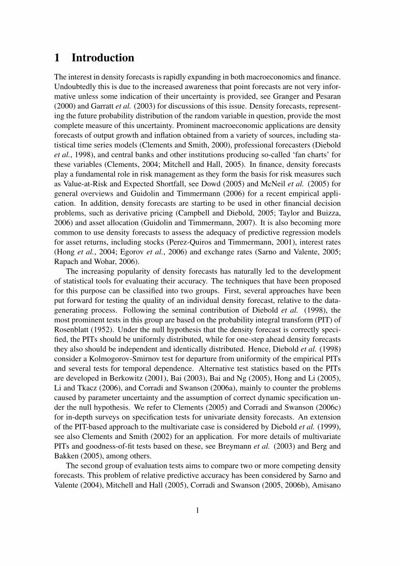
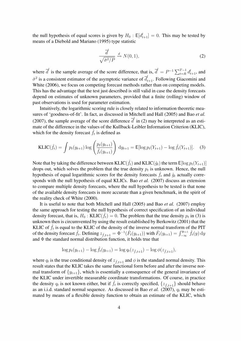
Figure 1: Probability density functions of the standard normal distribution ft(yt+1) and standard-ized Student-t(5) distribution gt(yt+1) (upper panel) and corresponding relative log-likelihoodscores log ft(yt+1)− log gt(yt+1) (lower panel).

The following example illustrates the issue at hand. Suppose we wish to compare theaccuracy of two density forecasts for Yt+1, one being the standard normal distribution withpdf

ft(yt+1) = (2π)−12 exp(−y2

t+1/2),

and the other being the (fat-tailed) Student-t distribution with ν degrees of freedom, stan-dardized to unit variance, with pdf

gt(yt+1) =Γ(

ν+12

)√(ν − 2)πΓ(ν

2)

(1 +

y2t+1

(ν − 2)

)−(ν+1)/2

with ν > 2.

Figure 1 shows these density functions for the case ν = 5, as well as the relative log-likelihood score log ft(yt+1) − log gt(yt+1). The score function is negative in the left tail(−∞, y∗), with y∗ ≈ −2.5. Now consider the average weighted log score d

wlas defined

before, based on an observed sample yR+1, . . . , yT of P observations from an unknowndensity on (−∞,∞) for which ft(yt+1) and gt(yt+1) are candidates. Using the thresholdweight function w(yt+1) = I(yt+1 ≤ r) to concentrate on the left tail, it follows fromthe lower panel of Figure 1 that if the threshold r < y∗, the average weighted log scorecan never be positive and will be strictly negative whenever there are observations in thetail. Evidently the test of equal predictive accuracy will then favor the fat-tailed Student-tdensity gt(yt+1), even if the true density is the standard normal ft(yt+1).

We emphasize that the problem sketched above is not limited to the logarithmic scor-ing rule but occurs more generally. For example, Berkowitz (2001) advocates the use

6

of the inverse normal transform zf ,t+1, as defined before, motivated by the fact that ifft is correctly specified, these should be an i.i.d. standard normal sequence. Taking thestandard normal log-likelihood of the transformed data leads to the following scoring rule:

SN(ft; yt+1) = log φ(zf ,t+1) = −1

2log(2π)− 1

2z2

f ,t+1. (6)

Although for a correctly specified density forecast the sequence zf ,t+1 is i.i.d. nor-mal, tests for the comparative accuracy of density forecasts in a particular region basedon the normal log-likelihood may be biased towards incorrect alternatives. A weightednormal scoring rule of the form

SwN(ft; yt+1) = w(yt+1) log φ(zf ,t+1) (7)

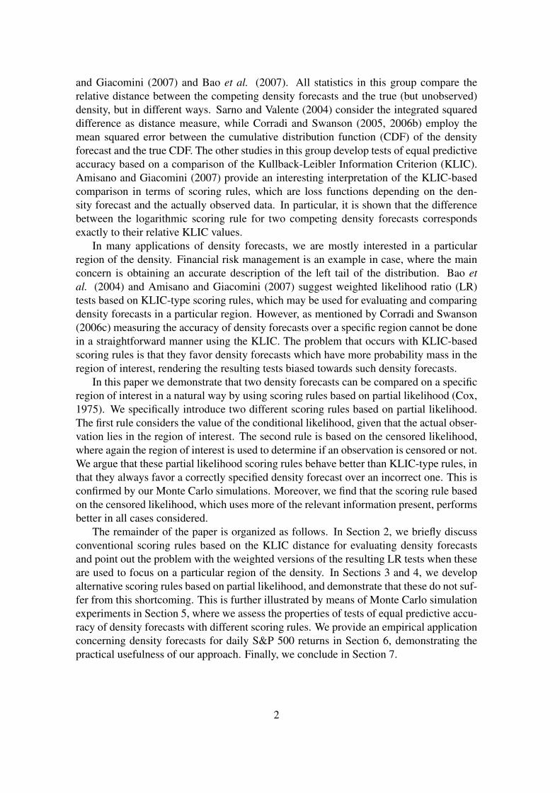
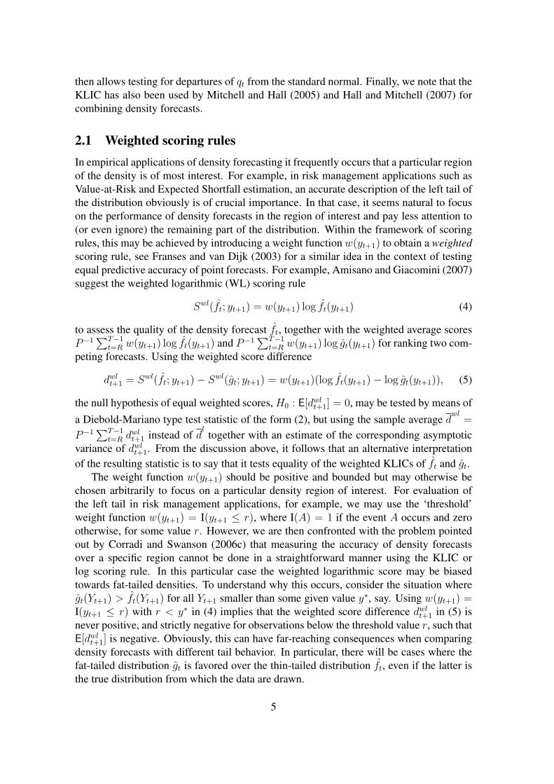
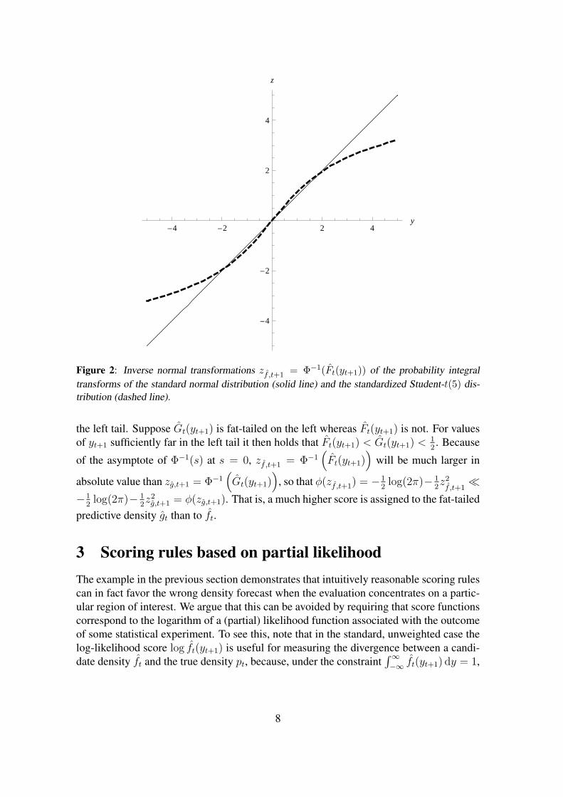
also would not guarantee that a correctly specified density forecast is preferred over anincorrectly specified density forecast. Figure 2 illustrates this point for standard normaland standardized Student-t(5) distributions, denoted as ft and gt as before. When focusingon the left tail by using the threshold weight function w(yt+1) = I(yt+1 ≤ r), it is seen that|zf ,t+1| > |zg,t+1| for all values of y less than y∗ ≈ −2. As for the weighted logarithmicscoring rule (4), it then follows that if the threshold r < y∗ the relative score dwN

t+1 =12w(yt+1)(z

2g,t+1 − z2

f ,t+1) is strictly negative for observations yt+1 in the left tail and zero

otherwise, such that the test based on the average score difference dwN

is biased againstthe Student-t alternative.

Berkowitz (2001) proposes a different way to use the scoring rule based on the normaltransform for evaluation of the accuracy of density forecasts in the left tail, based on theidea of censoring. Specifically, for a given quantile 0 < α < 1, define the censored normallog-likelihood (CNL) score function

ScN(ft, yt+1) = I(Ft(yt+1) < α) log φ(zf ,t+1) + I(Ft(yt+1) ≥ α) log(1− α)

= w(zf ,t+1) log φ(zf ,t+1) + (1− w(zf ,t+1)) log(1− α), (8)

where w(zf ,t+1) = I(zf ,t+1 < Φ−1(α)), which is equivalent to I(Ft(yt+1) < α). TheCNL scoring rule evaluates the shape of the density forecast for the region below the αthquantile and the frequency with which this region is visited. The latter form of (8) canalso be used to focus on other regions of interest by using a weight function w(Yt+1)equal to one in the region of interest, together with α bf,t = Pf ,t(w(Yt+1) = 1). One canarrange for the weight functions of competing density forecasts to coincide by allowingα to depend on the predictive density at hand. Particularly, in the case of the thresholdweight function the same threshold r can be used for two competing density forecasts byusing two different values of α, equal to the left exceedance probability of the value r forthe respective density forecast.

Although it is perfectly valid to assess the quality of an individual density forecast inan absolute sense based on (8), see Berkowitz (2001), this scoring rule should be used withcaution when testing the relative accuracy of competing density forecasts, as consideredby Bao et al. (2004). Like the WL scoring rule, the CNL scoring rule with the thresholdweight function has a tendency to favor predictive densities with more probability mass in

7

-4 -2 2 4y

-4

-2

2

4

z

Figure 2: Inverse normal transformations zf ,t+1 = Φ−1(Ft(yt+1)) of the probability integraltransforms of the standard normal distribution (solid line) and the standardized Student-t(5) dis-tribution (dashed line).

the left tail. Suppose Gt(yt+1) is fat-tailed on the left whereas Ft(yt+1) is not. For valuesof yt+1 sufficiently far in the left tail it then holds that Ft(yt+1) < Gt(yt+1) < 1

2. Because

of the asymptote of Φ−1(s) at s = 0, zf ,t+1 = Φ−1(Ft(yt+1)

)will be much larger in

absolute value than zg,t+1 = Φ−1(Gt(yt+1)

), so that φ(zf ,t+1) = −1

2log(2π)− 1

2z2

f ,t+1

−12log(2π)− 1

2z2

g,t+1 = φ(zg,t+1). That is, a much higher score is assigned to the fat-tailedpredictive density gt than to ft.

3 Scoring rules based on partial likelihoodThe example in the previous section demonstrates that intuitively reasonable scoring rulescan in fact favor the wrong density forecast when the evaluation concentrates on a partic-ular region of interest. We argue that this can be avoided by requiring that score functionscorrespond to the logarithm of a (partial) likelihood function associated with the outcomeof some statistical experiment. To see this, note that in the standard, unweighted case thelog-likelihood score log ft(yt+1) is useful for measuring the divergence between a candi-date density ft and the true density pt, because, under the constraint

∫∞−∞ ft(yt+1) dy = 1,

8

the expectation

EY [log ft(Yt+1)] ≡ E[log ft(Yt+1)|Yt+1 ∼ pt(yt+1)]

is maximized by taking ft = pt. This follows from the fact that for any density ft differentfrom pt we obtain

EY

[log

(ft(Yt+1)

pt(Yt+1)

)]≤ EY

[ft(Yt+1)

pt(Yt+1)

]− 1 =

∫ ∞

−∞pt(y)

ft(y)

pt(y)dy − 1 ≤ 0,

applying the inequality log x ≤ x− 1 to ft/pt.This shows that log-likelihood scores of different forecast methods can be compared in

a meaningful way, provided that the densities under consideration are properly normalizedto have unit total probability. The quality of a normalized density forecast ft can thereforebe quantified by the average score EY [log ft(Yt+1)]. If pt(y) is the true conditional densityof Yt+1, the KLIC is nonnegative and defines a divergence between the true and an approx-imate distribution. If the true data generating process is unknown, we can still use KLICdifferences to measure the relative performance of two competing densities, which rendersthe logarithmic score difference discussed before, dl

t+1 = log ft(yt+1)− log gt(yt+1).The implication from the above is that likelihood-based scoring rules may still be used

to assess the (relative) accuracy of density forecasts in a particular region of the distribu-tions, as long as the scoring rules correspond to (possibly partial) likelihood functions. Inthe specific case of the threshold weight function w(yt+1) = I(yt+1 ≤ r) we can breakdown the observation of Yt+1 in two stages. First, it is revealed whether Yt+1 is smallerthan the threshold value r or not. We introduce the random variable Vt+1 to denote theoutcome of this first stage experiment, defining it as

Vt+1 =

1 if Yt+1 ≤ r,0 if Yt+1 > r.

(9)

In the second stage the actual value Yt+1 is observed. The second stage experiment cor-responds to a draw from the conditional distribution of Yt+1 given the region (below orabove the threshold) in which Yt+1 lies according to the outcome of the first stage, asindicated by Vt+1. Note that we may easily allow for a time varying threshold value rt.However, this is not made explicit in the subsequent notation to keep the exposition assimple as possible.

Any (true or false) probability density function ft of Yt+1 given Ft can be written asthe product of the probability density function of Vt+1, which is revealed in the first stagebinomial experiment, and that of the second stage experiment in which Yt+1 is drawnfrom its conditional distribution given Vt+1. The likelihood function associated with theobserved values Vt+1 = I(Yt+1 ≤ r) = v and subsequently Yt+1 = y can thus be writtenas the product of the likelihood of Vt+1, which is a Bernoulli random variable with successprobability F (r), and that of the realization of Yt+1 given v:

(F (r))v(1− F (r))1−v

[f(y)

1− F (r)I(v = 0) +

f(y)

F (r)I(v = 1)

].

9

By disregarding either the information revealed by Vt+1 or Yt+1|v (possibly depending onthe first-stage outcome Vt+1) we can construct various partial likelihood functions. Thisenables us to formulate several scoring rules that may be viewed as weighted likelihoodscores. As these still can be interpreted as a true (albeit partial) likelihood, they can beused for comparing the predictive accuracy of different density forecasts. In the following,we discuss two specific scoring rules as examples.

Conditional likelihood scoring rule For a given density forecast ft, if we decide toignore information from the first stage and use the information revealed in the second stageonly if it turns out that Vt+1 = 1 (that is, if Yt is a tail event), we obtain the conditionallikelihood (CL) score function

Scl(ft; yt+1) = I(yt+1 ≤ r) log(ft(yt+1)/Ft(r)). (10)

The main argument for using such a score function would be to evaluate density fore-casts based on their behavior in the left tail (values less than or equal to r). However,due to the normalization of the total tail probability we lose information of the originaldensity forecast on how often tail observations actually occur. This is because the infor-mation regarding this frequency is revealed only by the first-stage experiment, which wehave explicitly ignored here. As a result, the conditional likelihood scoring rule attachescomparable scores to density forecasts that have similar tail shapes, but completely dif-ferent tail probabilities. This tail probability is obviously relevant for risk managementpurposes, in particular for Value-at-Risk evaluation. Hence, the following scoring ruletakes into account the tail behavior as well as the relative frequency with which the tail isvisited.

Censored likelihood scoring rule Combining the information revealed by the first stageexperiment with that of the second stage provided that Yt+1 is a tail event (Vt+1 = 1), weobtain the censored likelihood (CSL) score function

Scsl(ft; yt+1) = I(yt+1 ≤ r) log ft(yt+1) + I(yt+1 > r) log(1− Ft(r)). (11)

This scoring rule uses the information of the first stage (essentially information regardingthe CDF Ft(y) at y = r) but apart from that ignores the shape of ft(y) for values abovethe threshold value r. In that sense this scoring rule is similar to that used in the Tobitmodel for normally distributed random variables that cannot be observed above a certainthreshold value (see Tobin, 1958). To compare the censored likelihood score with thecensored normal score of (8), consider the case α = Ft(r) in the latter. The indicatorfuctions, as well as the second terms, in both scoring rules then coincide exactly, whilethe only difference between the scoring rules is that log ft(yt+1) occurs in the CSL rulein place where the CNL rule has log φ(zf ,t+1). It is the latter term that gave rise to the(too) high scores in the left tail to the standardized t(5)-distribution in case the correctdistribution is the standard normal.

We may test the null hypothesis of equal performance of two density forecasts ft(y)and gt(y) based on the conditional likelihood score (10) or the censored likelihood score(11) in the same manner as before. That is, given a sample of density forecasts and

10

0

0.2

0.4

0.6

0.8

1

-0.05 -0.025 0

em

piric

al C

DF

score

WLCNL

CLCSL

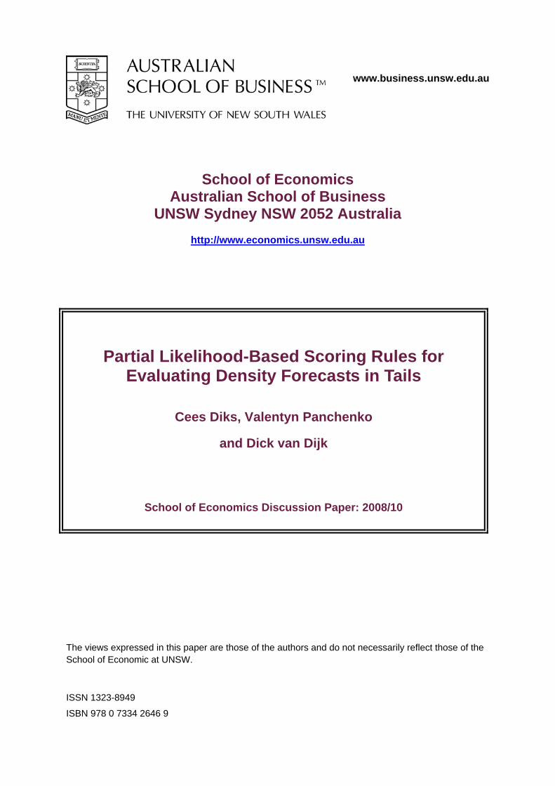
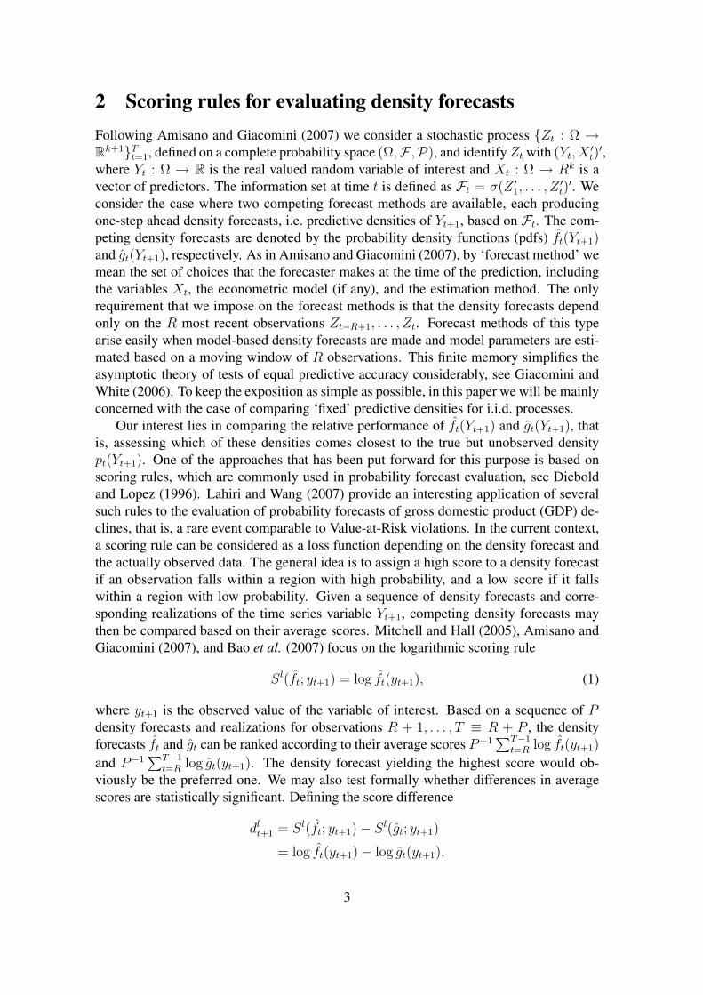
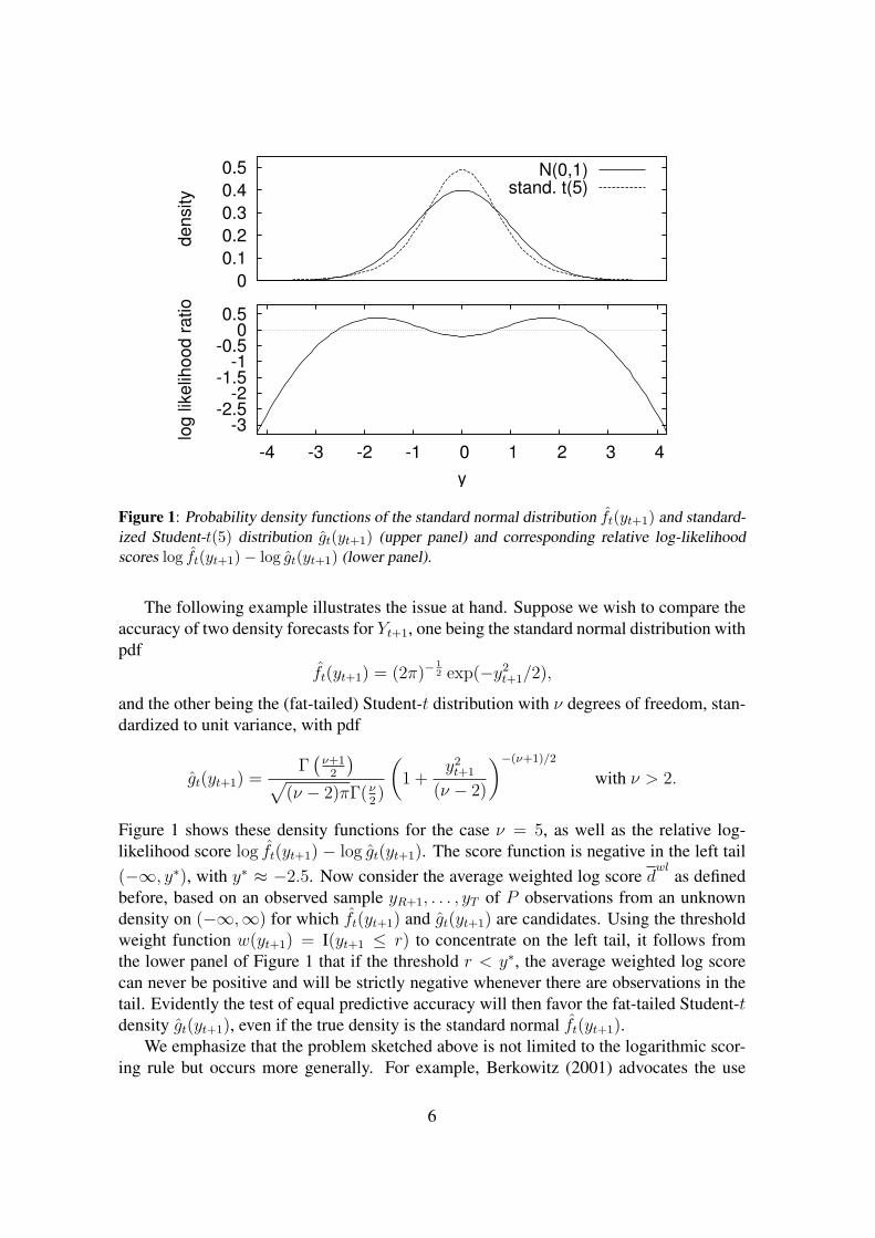
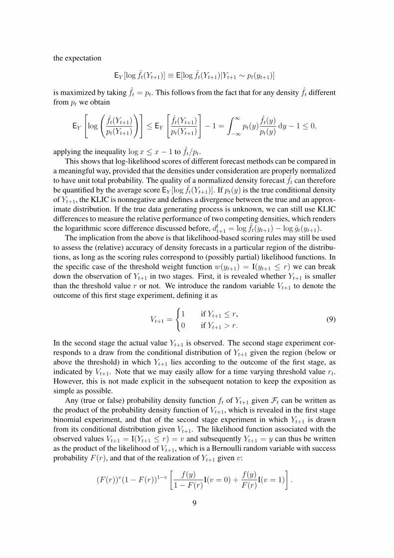
Figure 3: Empirical CDFs of mean relative scores d∗

for the weighted logarithmic (WL) scoringrule in (4), the censored normal likelihood (CNL) in (8), the conditional likelihood (CL) in (10),and the censored likelihood (CSL) in (11) for series of P = 2000 independent observations from astandard normal distribution. The scoring rules are based on the threshold weight function w(y) =I(y ≤ r) with r = −2.5. The relative score is defined as the score for (correct) standard normaldensity minus the score for the standardized Student-t(5) density. The graph is based on 10, 000replications.

corresponding realizations for P time periods R + 1, . . . , T , we may form the relativescores dcl

t+1 = Scl(ft; yt+1) − Scl(gt; yt+1) and dcslt+1 = Scsl(ft; yt+1) − Scsl(gt; yt+1) and

use these as the basis for computing a Diebold-Mariano type test statistic of the form givenin (2).

We revisit the example from the previous section in order to illustrate the properties ofthe various scoring rules and the associated tests for comparing the accuracy of competingdensity forecasts. We generate 10, 000 independent series of P = 2000 independentobservations yt+1 from a standard normal distribution. For each sequence we compute themean value of the weighted logarithmic scoring rule in (4), the censored normal likelihoodin (8), the conditional likelihood in (10), and the censored likelihood in (11). For the WLscoring rule score we use the threshold weight function w(yt+1) = I(yt+1 ≤ r), wherethe threshold is fixed at r = −2.5. The CNL score is used with α = Φ(r), where Φ(·)represents the standard normal CDF. The threshold value r = −2.5 is also used for the CLand CSL scores. Each scoring rule is computed for the (correct) standard normal densityft and the standardized Student-t density gt with five degrees of freedom.

Figure 3 shows the empirical CDF of the mean relative scores d∗, where ∗ is wl, cnl,

cl or csl. The average WL and CNL scores take almost exclusively negative values, whichmeans that for the weight function considered, on average they attach a lower score tothe correct normal distribution than to the Student-t distribution, leading to a bias in thecorresponding test statistic towards the incorrect, fat-tailed distribution. The two scoringrules based on partial likelihood both correctly favor the true normal density. The scores ofthe censored likelihood rule appear to be better at detecting the inadequacy of the Student-t distribution, in the sense that its relative scores stochastically dominate those based onthe conditional likelihood.

We close this section by noting that the validity of the CL and CSL scoring rules in (10)and (11) does not depend on the particular definition of Vt+1 (or weight function w(Yt+1))used. The two scoring rules discussed above focus on the case where Vt+1 = I(Yt+1 ≤

11

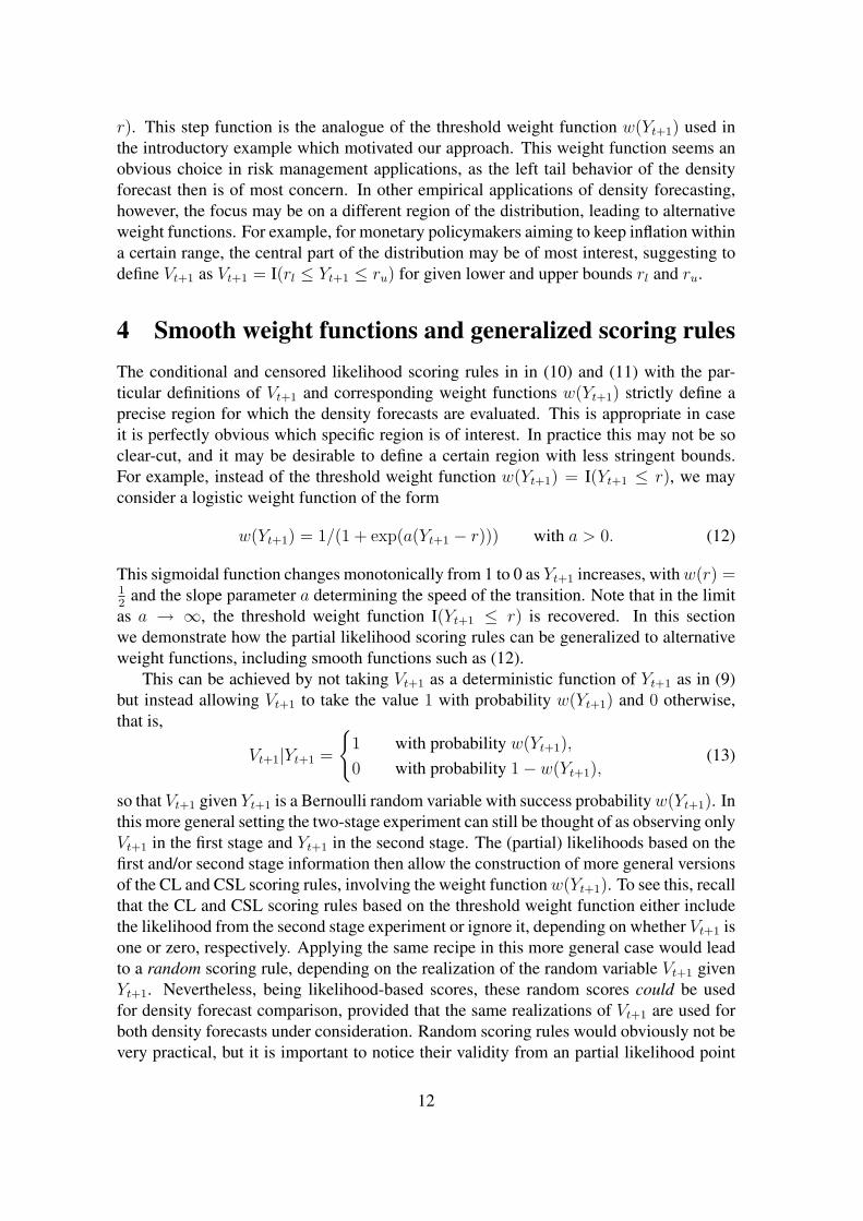
r). This step function is the analogue of the threshold weight function w(Yt+1) used inthe introductory example which motivated our approach. This weight function seems anobvious choice in risk management applications, as the left tail behavior of the densityforecast then is of most concern. In other empirical applications of density forecasting,however, the focus may be on a different region of the distribution, leading to alternativeweight functions. For example, for monetary policymakers aiming to keep inflation withina certain range, the central part of the distribution may be of most interest, suggesting todefine Vt+1 as Vt+1 = I(rl ≤ Yt+1 ≤ ru) for given lower and upper bounds rl and ru.

4 Smooth weight functions and generalized scoring rulesThe conditional and censored likelihood scoring rules in in (10) and (11) with the par-ticular definitions of Vt+1 and corresponding weight functions w(Yt+1) strictly define aprecise region for which the density forecasts are evaluated. This is appropriate in caseit is perfectly obvious which specific region is of interest. In practice this may not be soclear-cut, and it may be desirable to define a certain region with less stringent bounds.For example, instead of the threshold weight function w(Yt+1) = I(Yt+1 ≤ r), we mayconsider a logistic weight function of the form

w(Yt+1) = 1/(1 + exp(a(Yt+1 − r))) with a > 0. (12)

This sigmoidal function changes monotonically from 1 to 0 as Yt+1 increases, with w(r) =12

and the slope parameter a determining the speed of the transition. Note that in the limitas a → ∞, the threshold weight function I(Yt+1 ≤ r) is recovered. In this sectionwe demonstrate how the partial likelihood scoring rules can be generalized to alternativeweight functions, including smooth functions such as (12).

This can be achieved by not taking Vt+1 as a deterministic function of Yt+1 as in (9)but instead allowing Vt+1 to take the value 1 with probability w(Yt+1) and 0 otherwise,that is,

Vt+1|Yt+1 =

1 with probability w(Yt+1),

0 with probability 1− w(Yt+1),(13)

so that Vt+1 given Yt+1 is a Bernoulli random variable with success probability w(Yt+1). Inthis more general setting the two-stage experiment can still be thought of as observing onlyVt+1 in the first stage and Yt+1 in the second stage. The (partial) likelihoods based on thefirst and/or second stage information then allow the construction of more general versionsof the CL and CSL scoring rules, involving the weight function w(Yt+1). To see this, recallthat the CL and CSL scoring rules based on the threshold weight function either includethe likelihood from the second stage experiment or ignore it, depending on whether Vt+1 isone or zero, respectively. Applying the same recipe in this more general case would leadto a random scoring rule, depending on the realization of the random variable Vt+1 givenYt+1. Nevertheless, being likelihood-based scores, these random scores could be usedfor density forecast comparison, provided that the same realizations of Vt+1 are used forboth density forecasts under consideration. Random scoring rules would obviously not bevery practical, but it is important to notice their validity from an partial likelihood point

12

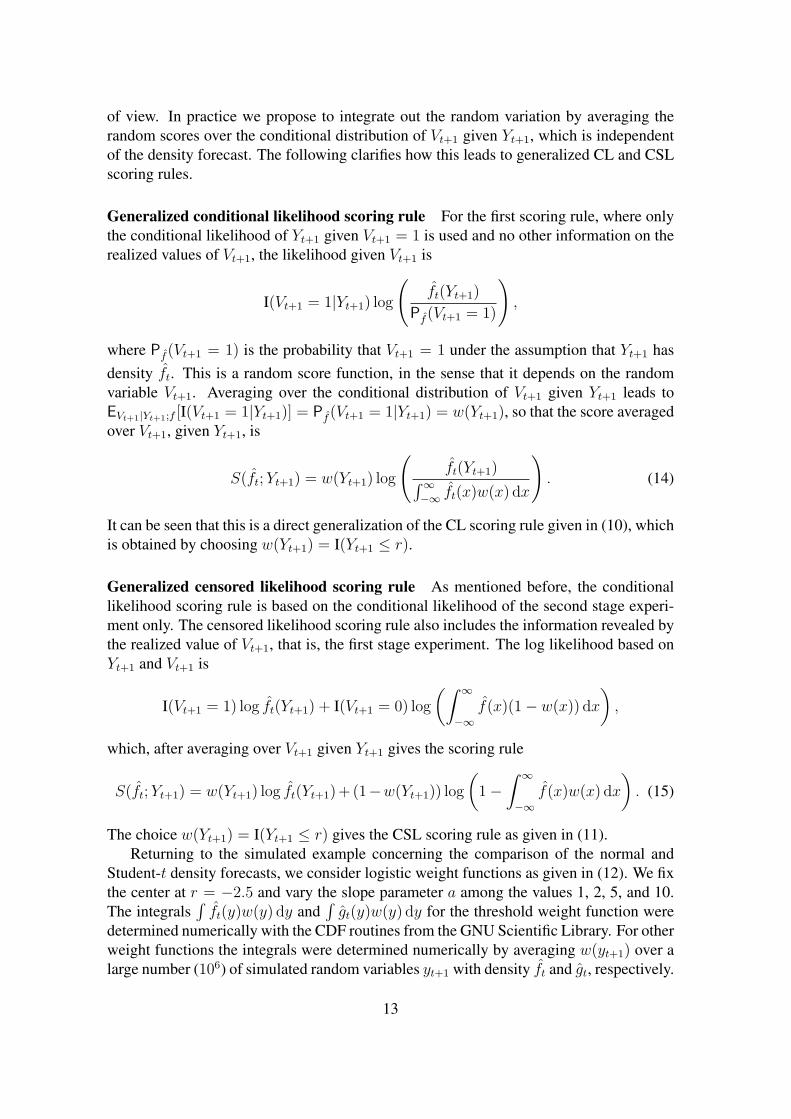
of view. In practice we propose to integrate out the random variation by averaging therandom scores over the conditional distribution of Vt+1 given Yt+1, which is independentof the density forecast. The following clarifies how this leads to generalized CL and CSLscoring rules.

Generalized conditional likelihood scoring rule For the first scoring rule, where onlythe conditional likelihood of Yt+1 given Vt+1 = 1 is used and no other information on therealized values of Vt+1, the likelihood given Vt+1 is

I(Vt+1 = 1|Yt+1) log

(ft(Yt+1)

Pf (Vt+1 = 1)

),

where Pf (Vt+1 = 1) is the probability that Vt+1 = 1 under the assumption that Yt+1 hasdensity ft. This is a random score function, in the sense that it depends on the randomvariable Vt+1. Averaging over the conditional distribution of Vt+1 given Yt+1 leads toEVt+1|Yt+1;f [I(Vt+1 = 1|Yt+1)] = Pf (Vt+1 = 1|Yt+1) = w(Yt+1), so that the score averagedover Vt+1, given Yt+1, is

S(ft; Yt+1) = w(Yt+1) log

(ft(Yt+1)∫∞

−∞ ft(x)w(x) dx

). (14)

It can be seen that this is a direct generalization of the CL scoring rule given in (10), whichis obtained by choosing w(Yt+1) = I(Yt+1 ≤ r).

Generalized censored likelihood scoring rule As mentioned before, the conditionallikelihood scoring rule is based on the conditional likelihood of the second stage experi-ment only. The censored likelihood scoring rule also includes the information revealed bythe realized value of Vt+1, that is, the first stage experiment. The log likelihood based onYt+1 and Vt+1 is

I(Vt+1 = 1) log ft(Yt+1) + I(Vt+1 = 0) log

(∫ ∞

−∞f(x)(1− w(x)) dx

),

which, after averaging over Vt+1 given Yt+1 gives the scoring rule

S(ft; Yt+1) = w(Yt+1) log ft(Yt+1)+ (1−w(Yt+1)) log

(1−

∫ ∞

−∞f(x)w(x) dx

). (15)

The choice w(Yt+1) = I(Yt+1 ≤ r) gives the CSL scoring rule as given in (11).Returning to the simulated example concerning the comparison of the normal and

Student-t density forecasts, we consider logistic weight functions as given in (12). We fixthe center at r = −2.5 and vary the slope parameter a among the values 1, 2, 5, and 10.The integrals

∫ft(y)w(y) dy and

∫gt(y)w(y) dy for the threshold weight function were

determined numerically with the CDF routines from the GNU Scientific Library. For otherweight functions the integrals were determined numerically by averaging w(yt+1) over alarge number (106) of simulated random variables yt+1 with density ft and gt, respectively.

13

0

0.2

0.4

0.6

0.8

1

0 0.01 0.02 0.03 0.04

em

piric

al C

DF

score

(a=1)

CLCSL

0

0.2

0.4

0.6

0.8

1

0 0.01 0.02 0.03 0.04

em

piric

al C

DF

score

(a=2)

CLCSL

0

0.2

0.4

0.6

0.8

1

0 0.01 0.02 0.03 0.04

em

piric

al C

DF

score

(a=5)

CLCSL

0

0.2

0.4

0.6

0.8

1

0 0.01 0.02 0.03 0.04

em

piric

al C

DF

score

(a=10)

CLCSL

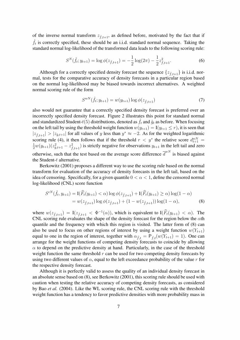
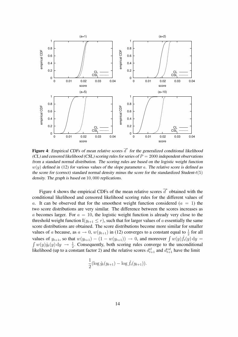
Figure 4: Empirical CDFs of mean relative scores d∗

for the generalized conditional likelihood(CL) and censored likelihood (CSL) scoring rules for series of P = 2000 independent observationsfrom a standard normal distribution. The scoring rules are based on the logistic weight functionw(y) defined in (12) for various values of the slope parameter a. The relative score is defined asthe score for (correct) standard normal density minus the score for the standardized Student-t(5)density. The graph is based on 10, 000 replications.

Figure 4 shows the empirical CDFs of the mean relative scores d∗

obtained with theconditional likelihood and censored likelihood scoring rules for the different values ofa. It can be observed that for the smoothest weight function considered (a = 1) thetwo score distributions are very similar. The difference between the scores increases asa becomes larger. For a = 10, the logistic weight function is already very close to thethreshold weight function I(yt+1 ≤ r), such that for larger values of a essentially the samescore distributions are obtained. The score distributions become more similar for smallervalues of a because, as a → 0, w(yt+1) in (12) converges to a constant equal to 1

2for all

values of yt+1, so that w(yt+1) − (1 − w(yt+1)) → 0, and moreover∫

w(y)ft(y) dy =∫w(y)gt(y) dy → 1

2. Consequently, both scoring rules converge to the unconditional

likelihood (up to a constant factor 2) and the relative scores dclt+1 and dcsl

t+1 have the limit

1

2(log gt(yt+1)− log ft(yt+1)).

14

5 Monte Carlo simulationsIn this section we examine the implications of using the weighted logarithmic scoringrule in (4), the censored normal likelihood in (8), the conditional likelihood in (10), andthe censored likelihood in (11) for constructing a test of equal predictive ability of twocompeting density forecasts. Specifically, we consider the size and power properties ofthe Diebold-Mariano type test as given in (2). The null hypothesis states that the twocompeting density forecasts have equal expected scores, or

H0 : E[d∗t+1] = 0,

under scoring rule ∗, where ∗ is either wl, cnl, cl or csl. We focus on one-sided rejectionrates to highlight the fact that some of the scoring rules may favor a wrongly specifieddensity forecast over a correctly specified one. Throughout we use a HAC-estimator forthe asymptotic variance of the relative score d∗t+1, that is σ2 = γ0 + 2

∑K−1k=1 akγk, where

γk denotes the lag-k sample covariance of the sequence d∗t+1T−1t=R and ak are the Bartlett

weights ak = 1− k/K with K = bP−1/4c, where P = T −R is the sample size.

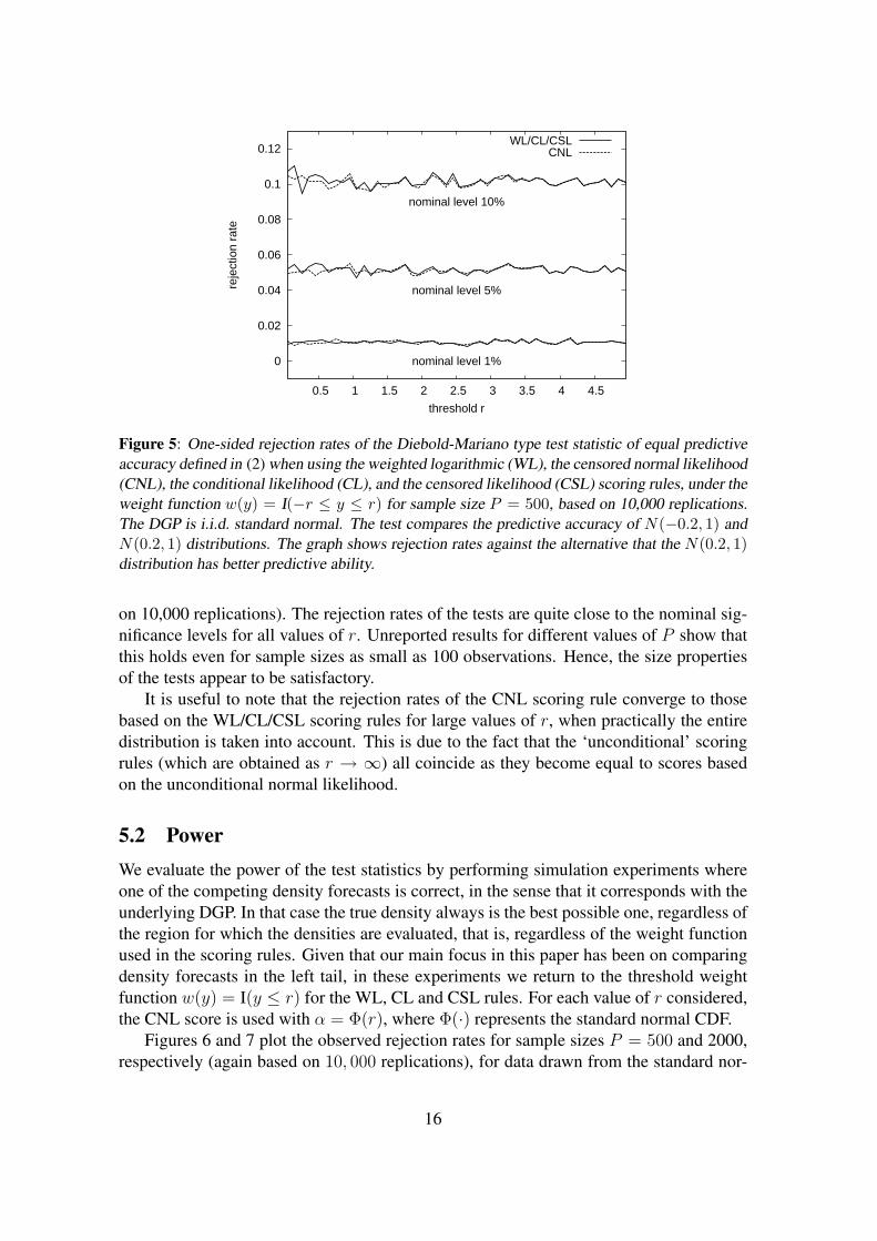
5.1 SizeIn order to assess the size properties of the tests a case is required with two competingpredictive densities that are both ‘equally (in)correct’. However, whether or not the nullhypothesis of equal predictive ability holds depends on the weight function w(yt+1) that isused in the scoring rules. This complicates the simulation design, also given the fact thatwe would like to examine how the behavior of the tests depends on the specific settings ofthe weight function. For the threshold weight function w(yt+1) = I(yt+1 ≤ r) it appears tobe impossible to construct an example with two different density forecasts having identicalpredictive ability regardless of the value of r. We therefore evaluate the size of the tests byfocusing on the central part of the distribution using the weight function w(y) = I(−r ≤y ≤ r). As mentioned before, in some cases this region of the distribution may be ofprimary interest, for instance to monetary policymakers aiming to keep inflation betweencertain lower and upper bounds. The data generating process (DGP) is taken to be ani.i.d. standard normal distribution, while the two competing density forecasts are normaldistributions with means equal to −0.2 and 0.2, and variance equal to 1. In this case,independent of the value of r the competing density forecasts have equal predictive ability,as the scoring rules considered here are invariant under a simultaneous reflection aboutzero of all densities of interest (the true conditional density as well as the two competingdensity forecasts under consideration). In addition, it turns out that for this combinationof DGP and predictive densities, the relative scores d∗t+1 for the WL, CL and CSL rulesbased on w(y) = I(−r ≤ y ≤ r) are identical. For this weight function the CNL ruletakes the form of the last expression in (8), with α = Pt(Yt+1 = 1) = P(−r ≤ Yt+1 ≤r) = Φ(r)− Φ(−r).

Figure 5 displays one-sided rejection rates (at nominal significance levels of 1, 5 and10%) of the null hypothesis against the alternative that the N(0.2, 1) distribution has betterpredictive ability as a function of the threshold value r, for sample size P = 500 (based

15

0

0.02

0.04

0.06

0.08

0.1

0.12

0.5 1 1.5 2 2.5 3 3.5 4 4.5

reje

ctio

n ra

te

threshold r

nominal level 1%

nominal level 5%

nominal level 10%

WL/CL/CSLCNL

Figure 5: One-sided rejection rates of the Diebold-Mariano type test statistic of equal predictiveaccuracy defined in (2) when using the weighted logarithmic (WL), the censored normal likelihood(CNL), the conditional likelihood (CL), and the censored likelihood (CSL) scoring rules, under theweight function w(y) = I(−r ≤ y ≤ r) for sample size P = 500, based on 10,000 replications.The DGP is i.i.d. standard normal. The test compares the predictive accuracy of N(−0.2, 1) andN(0.2, 1) distributions. The graph shows rejection rates against the alternative that the N(0.2, 1)distribution has better predictive ability.

on 10,000 replications). The rejection rates of the tests are quite close to the nominal sig-nificance levels for all values of r. Unreported results for different values of P show thatthis holds even for sample sizes as small as 100 observations. Hence, the size propertiesof the tests appear to be satisfactory.

It is useful to note that the rejection rates of the CNL scoring rule converge to thosebased on the WL/CL/CSL scoring rules for large values of r, when practically the entiredistribution is taken into account. This is due to the fact that the ‘unconditional’ scoringrules (which are obtained as r → ∞) all coincide as they become equal to scores basedon the unconditional normal likelihood.

5.2 PowerWe evaluate the power of the test statistics by performing simulation experiments whereone of the competing density forecasts is correct, in the sense that it corresponds with theunderlying DGP. In that case the true density always is the best possible one, regardless ofthe region for which the densities are evaluated, that is, regardless of the weight functionused in the scoring rules. Given that our main focus in this paper has been on comparingdensity forecasts in the left tail, in these experiments we return to the threshold weightfunction w(y) = I(y ≤ r) for the WL, CL and CSL rules. For each value of r considered,the CNL score is used with α = Φ(r), where Φ(·) represents the standard normal CDF.

Figures 6 and 7 plot the observed rejection rates for sample sizes P = 500 and 2000,respectively (again based on 10, 000 replications), for data drawn from the standard nor-

16

0

0.2

0.4

0.6

0.8

1

-4 -2 0 2 4

reje

ctio

n ra

te

threshold r

WLCNL

CLCSL

0

0.2

0.4

0.6

0.8

1

-4 -2 0 2 4

reje

ctio

n ra

te

threshold r

WLCNL

CLCSL

0

0.2

0.4

0.6

0.8

1

-4 -2 0 2 4

reje

ctio

n ra

te

threshold r

WLCNL

CLCSL

0

0.2

0.4

0.6

0.8

1

-4 -2 0 2 4

reje

ctio

n ra

te

threshold r

WLCNL

CLCSL

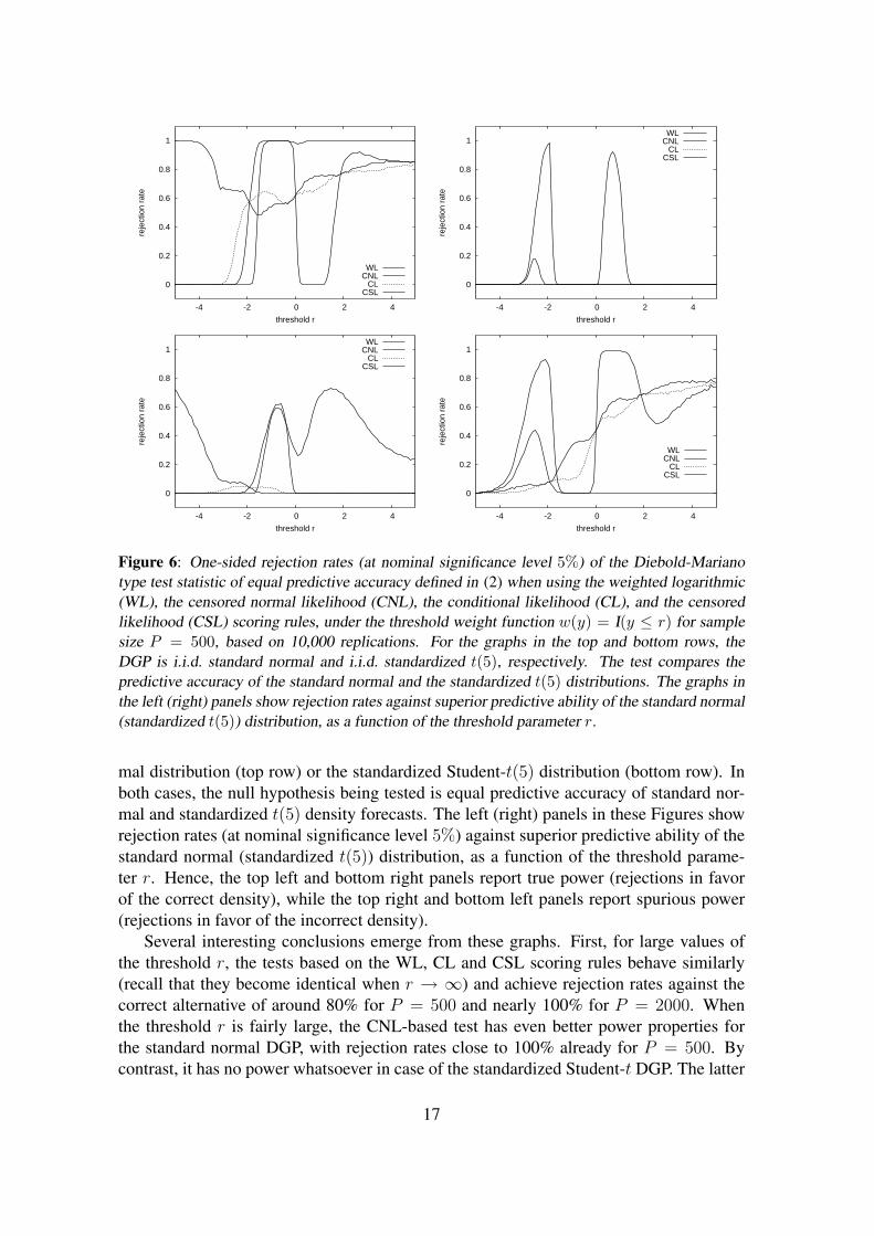
Figure 6: One-sided rejection rates (at nominal significance level 5%) of the Diebold-Marianotype test statistic of equal predictive accuracy defined in (2) when using the weighted logarithmic(WL), the censored normal likelihood (CNL), the conditional likelihood (CL), and the censoredlikelihood (CSL) scoring rules, under the threshold weight function w(y) = I(y ≤ r) for samplesize P = 500, based on 10,000 replications. For the graphs in the top and bottom rows, theDGP is i.i.d. standard normal and i.i.d. standardized t(5), respectively. The test compares thepredictive accuracy of the standard normal and the standardized t(5) distributions. The graphs inthe left (right) panels show rejection rates against superior predictive ability of the standard normal(standardized t(5)) distribution, as a function of the threshold parameter r.

mal distribution (top row) or the standardized Student-t(5) distribution (bottom row). Inboth cases, the null hypothesis being tested is equal predictive accuracy of standard nor-mal and standardized t(5) density forecasts. The left (right) panels in these Figures showrejection rates (at nominal significance level 5%) against superior predictive ability of thestandard normal (standardized t(5)) distribution, as a function of the threshold parame-ter r. Hence, the top left and bottom right panels report true power (rejections in favorof the correct density), while the top right and bottom left panels report spurious power(rejections in favor of the incorrect density).

Several interesting conclusions emerge from these graphs. First, for large values ofthe threshold r, the tests based on the WL, CL and CSL scoring rules behave similarly(recall that they become identical when r → ∞) and achieve rejection rates against thecorrect alternative of around 80% for P = 500 and nearly 100% for P = 2000. Whenthe threshold r is fairly large, the CNL-based test has even better power properties forthe standard normal DGP, with rejection rates close to 100% already for P = 500. Bycontrast, it has no power whatsoever in case of the standardized Student-t DGP. The latter

17

0

0.2

0.4

0.6

0.8

1

-4 -2 0 2 4

reje

ctio

n ra

te

threshold r

WLCNL

CLCSL

0

0.2

0.4

0.6

0.8

1

-4 -2 0 2 4

reje

ctio

n ra

te

threshold r

WLCNL

CLCSL

0

0.2

0.4

0.6

0.8

1

-4 -2 0 2 4

reje

ctio

n ra

te

threshold r

WLCNL

CLCSL

0

0.2

0.4

0.6

0.8

1

-4 -2 0 2 4

reje

ctio

n ra

te

threshold r

WLCNL

CLCSL

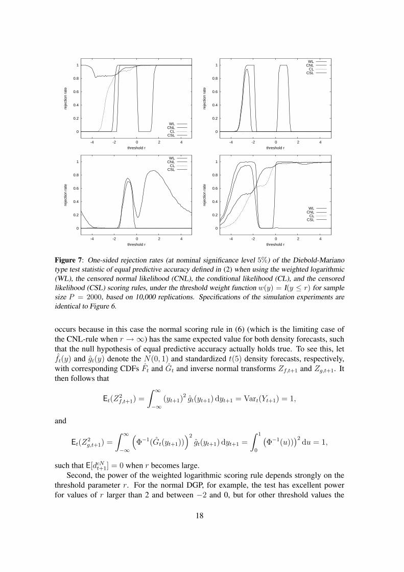
Figure 7: One-sided rejection rates (at nominal significance level 5%) of the Diebold-Marianotype test statistic of equal predictive accuracy defined in (2) when using the weighted logarithmic(WL), the censored normal likelihood (CNL), the conditional likelihood (CL), and the censoredlikelihood (CSL) scoring rules, under the threshold weight function w(y) = I(y ≤ r) for samplesize P = 2000, based on 10,000 replications. Specifications of the simulation experiments areidentical to Figure 6.

occurs because in this case the normal scoring rule in (6) (which is the limiting case ofthe CNL-rule when r →∞) has the same expected value for both density forecasts, suchthat the null hypothesis of equal predictive accuracy actually holds true. To see this, letft(y) and gt(y) denote the N(0, 1) and standardized t(5) density forecasts, respectively,with corresponding CDFs Ft and Gt and inverse normal transforms Zf,t+1 and Zg,t+1. Itthen follows that

Et(Z2f,t+1) =

∫ ∞

−∞(yt+1)

2 gt(yt+1) dyt+1 = Vart(Yt+1) = 1,

and

Et(Z2g,t+1) =

∫ ∞

−∞

(Φ−1(Gt(yt+1))

)2

gt(yt+1) dyt+1 =

∫ 1

0

(Φ−1(u))

)2du = 1,

such that E[dcNt+1] = 0 when r becomes large.

Second, the power of the weighted logarithmic scoring rule depends strongly on thethreshold parameter r. For the normal DGP, for example, the test has excellent powerfor values of r larger than 2 and between −2 and 0, but for other threshold values the

18

-0.03

-0.02

-0.01

0

0.01

0.02

0.03

0.04

0.05

-4 -2 0 2 4

mea

n sc

ore

r

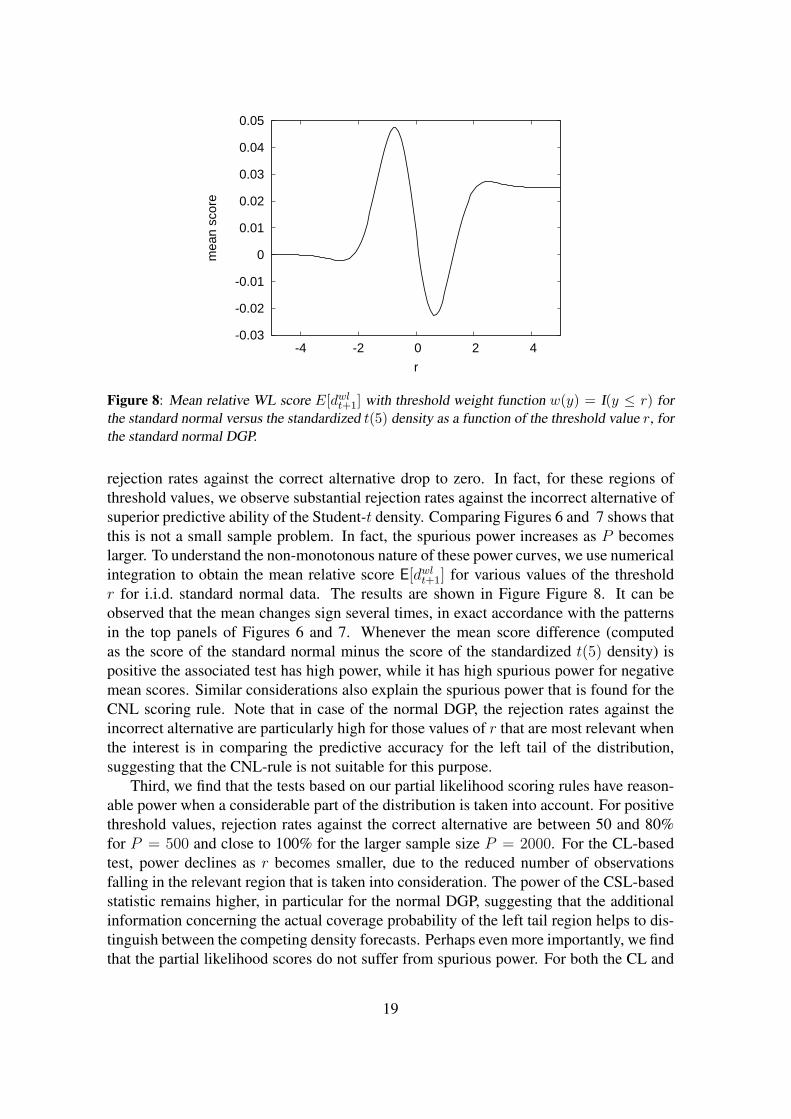
Figure 8: Mean relative WL score E[dwlt+1] with threshold weight function w(y) = I(y ≤ r) for

the standard normal versus the standardized t(5) density as a function of the threshold value r, forthe standard normal DGP.

rejection rates against the correct alternative drop to zero. In fact, for these regions ofthreshold values, we observe substantial rejection rates against the incorrect alternative ofsuperior predictive ability of the Student-t density. Comparing Figures 6 and 7 shows thatthis is not a small sample problem. In fact, the spurious power increases as P becomeslarger. To understand the non-monotonous nature of these power curves, we use numericalintegration to obtain the mean relative score E[dwl

t+1] for various values of the thresholdr for i.i.d. standard normal data. The results are shown in Figure Figure 8. It can beobserved that the mean changes sign several times, in exact accordance with the patternsin the top panels of Figures 6 and 7. Whenever the mean score difference (computedas the score of the standard normal minus the score of the standardized t(5) density) ispositive the associated test has high power, while it has high spurious power for negativemean scores. Similar considerations also explain the spurious power that is found for theCNL scoring rule. Note that in case of the normal DGP, the rejection rates against theincorrect alternative are particularly high for those values of r that are most relevant whenthe interest is in comparing the predictive accuracy for the left tail of the distribution,suggesting that the CNL-rule is not suitable for this purpose.

Third, we find that the tests based on our partial likelihood scoring rules have reason-able power when a considerable part of the distribution is taken into account. For positivethreshold values, rejection rates against the correct alternative are between 50 and 80%for P = 500 and close to 100% for the larger sample size P = 2000. For the CL-basedtest, power declines as r becomes smaller, due to the reduced number of observationsfalling in the relevant region that is taken into consideration. The power of the CSL-basedstatistic remains higher, in particular for the normal DGP, suggesting that the additionalinformation concerning the actual coverage probability of the left tail region helps to dis-tinguish between the competing density forecasts. Perhaps even more importantly, we findthat the partial likelihood scores do not suffer from spurious power. For both the CL and

19

0

0.2

0.4

0.6

0.8

1

0.5 1 1.5 2 2.5 3 3.5 4 4.5

reje

ctio

n ra

te

threshold r

WLCNL

CLCSL

0

0.2

0.4

0.6

0.8

1

0.5 1 1.5 2 2.5 3 3.5 4 4.5

reje

ctio

n ra

te

threshold r

WLCNL

CLCSL

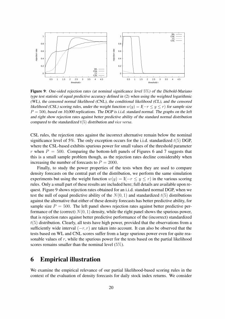
Figure 9: One-sided rejection rates (at nominal significance level 5%) of the Diebold-Marianotype test statistic of equal predictive accuracy defined in (2) when using the weighted logarithmic(WL), the censored normal likelihood (CNL), the conditional likelihood (CL), and the censoredlikelihood (CSL) scoring rules, under the weight function w(y) = I(−r ≤ y ≤ r) for sample sizeP = 500, based on 10,000 replications. The DGP is i.i.d. standard normal. The graphs on the leftand right show rejection rates against better predictive ability of the standard normal distributioncompared to the standardized t(5) distribution and vice versa.

CSL rules, the rejection rates against the incorrect alternative remain below the nominalsignificance level of 5%. The only exception occurs for the i.i.d. standardized t(5) DGP,where the CSL-based exhibits spurious power for small values of the threshold parameterr when P = 500. Comparing the bottom-left panels of Figures 6 and 7 suggests thatthis is a small sample problem though, as the rejection rates decline considerably whenincreasing the number of forecasts to P = 2000.

Finally, to study the power properties of the tests when they are used to comparedensity forecasts on the central part of the distribution, we perform the same simulationexperiments but using the weight function w(y) = I(−r ≤ y ≤ r) in the various scoringrules. Only a small part of these results are included here; full details are available upon re-quest. Figure 9 shows rejection rates obtained for an i.i.d. standard normal DGP, when wetest the null of equal predictive ability of the N(0, 1) and standardized t(5) distributionsagainst the alternative that either of these density forecasts has better predictive ability, forsample size P = 500. The left panel shows rejection rates against better predictive per-formance of the (correct) N(0, 1) density, while the right panel shows the spurious power,that is rejection rates against better predictive performance of the (incorrect) standardizedt(5) distribution. Clearly, all tests have high power, provided that the observations from asufficiently wide interval (−r, r) are taken into account. It can also be observed that thetests based on WL and CNL scores suffer from a large spurious power even for quite rea-sonable values of r, while the spurious power for the tests based on the partial likelihoodscores remains smaller than the nominal level (5%).

6 Empirical illustrationWe examine the empirical relevance of our partial likelihood-based scoring rules in thecontext of the evaluation of density forecasts for daily stock index returns. We consider

20

S&P 500 log-returns yt = ln(Pt/Pt−1), where Pt is the closing price on day t, adjustedfor dividends and stock splits. The sample period runs from January 1, 1980 until March14, 2008, giving a total of 7115 observations (source: Datastream).

For illustrative purposes we define two forecast methods based on GARCH modelsin such a way that a priori one of the methods is expected to be superior to the other.Examining a large variety of GARCH specifications for forecasting daily US stock indexreturns, Bao et al. (2007) conclude that the accuracy of density forecasts depends moreon the choice of the distribution of the standardized innovations than on the choice ofthe volatility specification. Therefore, we differentiate our forecast methods in terms ofthe innovation distribution, while keeping identical specifications for the conditional meanand the conditional variance. We consider an AR(5) model for the conditional mean returntogether with a GARCH(1,1) model for the conditional variance, that is

yt = µt + εt = µt +√

htηt,

where the conditional mean µt and the conditional variance ht are given by

µt = ρ0 +5∑

j=1

ρjyt−j,

ht = ω + αε2t−1 + βht−1,

and the standardized innovations ηt are i.i.d. with mean zero and variance one.Following Bollerslev (1987), a common finding in empirical applications has been

that GARCH models with a normal distribution for ηt are not able to fully account for thekurtosis observed in stock returns. We therefore concentrate on leptokurtic distributionsfor the standardized innovations. Specifically, for one forecast method the distribution ofηt is specified as a (standardized) Student-t distribution with ν degrees of freedom, whilefor the other forecast method we use the (standardized) Laplace distribution. Note that forthe Student-t distribution the degrees of freedom ν is a parameter that is to be estimated.The degrees of freedom directly determines the value of the excess kurtosis of the stan-dardized innovations, which is equal to 6/(ν− 4) (assuming ν > 4). Due to its flexibility,the Student-t distribution has been widely used in GARCH modeling (see e.g. Bollerslev(1987), Baillie and Bollerslev (1989)). The standardized Laplace distribution provides amore parsimonious alternative with no additional parameters to be estimated and has beenapplied in the context of conditional volatility modeling by Granger and Ding (1995) andMittnik et al. (1998)). The Laplace distribution has excess kurtosis of 3, which exceedsthe excess kurtosis of the Student-t(ν) distribution for ν > 6. Because of the greaterflexibility in modeling kurtosis, we may expect that the forecast method with Student-tinnovations gives superior density forecasts relative to the Laplace innovations. This isindeed indicated by results in Bao et al. (2007), who evaluate these density forecasts‘unconditionally’, that is, not focusing on a particular region of the distribution.

Our evaluation of the two forecast methods is based on their one-step ahead densityforecasts for returns, using a rolling window scheme for parameter estimation. The widthof the estimation window is set to R = 2000 observations, so that the number of out-of-sample observations is equal to P = 5115. For comparing the density forecasts’ accuracy

21

we use the Diebold-Mariano type test based on the weighted logarithmic scoring rulein (4), the censored normal likelihood in (8), the conditional likelihood in (10), and thecensored likelihood in (11). We concentrate on the left tail of the distribution by using thethreshold weight function w(yt+1) = I(yt+1 ≤ rt) for the WL, CL and CSL scoring rules.We consider two time-varying thresholds rt, that are determined as the one-day Value-at-Risk estimates at the 95% and 99% level based on the corresponding quantiles of theempirical CDF of the return observations in the relevant estimation window. For the CNLscoring rule in (8) we use the corresponding values α = 0.05 and 0.01, respectively. Thescore difference d∗t+1 is computed by subtracting the score of the GARCH-Laplace densityforecast from the score of the GARCH-t density forecast, such that positive values of d∗t+1

indicate better predictive ability of the forecast method based on Student-t innovations.Table 1 shows the average score differences d

∗with the accompanying tests of equal

predictive accuracy as in (2), where we use a HAC estimator for the asymptotic varianceσ2 to account for serial dependence in the d∗t+1 series. The results clearly demonstratethat different conclusions follow from the different scoring rules. For both choices ofthe threshold rt the WL and CNL scoring rules suggest superior predictive ability of theforecast method based on Laplace innovations. By contrast, the CL scoring rule suggeststhat the performance of the GARCH-t density forecasts is superior. The CSL scoringrule points towards the same conclusion as the CL rule, although the evidence for betterpredictive ability of the GARCH-t specification is somewhat weaker. In the remainder ofthis section we seek to understand the reasons for these conflicting results, and explorethe consequences of selecting either forecast method for risk management purposes. Inaddition, this allows us to obtain circumstantial evidence that shows which of the twocompeting forecast methods is most appropriate.

For most estimation windows, the degrees of freedom parameter in the Student-t dis-tribution is estimated to be (slightly) larger than 6, such that the Laplace distribution im-plies fatter tails than the Student-t distribution. Hence, it may very well be that the WLand CNL scoring rules indicate superior predictive ability of the Laplace distribution sim-ply because this density has more probability mass in the region of interest, that is, theproblem that motivated our analysis in the first place. To see this from a slightly differ-ent perspective, we compute one-day 95% and 99% Value-at-Risk (VaR) and ExpectedShortfall (ES) estimates as implied by the two forecast methods. The 100 × (1 − α)%Value-at-Risk is determined as the α-th quantile of the density forecast ft, that is, throughPf ,t

(Yt+1 ≤ VaRf ,t(α)

)= α. The Expected Shortfall is defined as the conditional mean

return given that Yt+1 ≤ VaRf ,t(α), that is ESf ,t(α) = Ef ,t

(Yt+1|Yt+1 ≤ VaRf ,t(α)

).

Figure 10 shows the VaR estimates against the realized returns. We observe that typicallythe VaR estimates based on the Laplace innovations are more extreme and, thus, implyfatter tails than the Student-t innovations. The same conclusion follows from the sampleaverages of the VaR and ES estimates, as shown in Table 2.

The VaR and ES estimates also enable us to assess which of the two innovation distri-butions is the most appropriate in a different way. For that purpose, we first of all computethe frequency of 95% and 99% VaR violations, which should be close to 0.05 and 0.01,respectively, if the innovation distribution is correctly specified. We compute the likeli-hood ratio (LR) test of correct unconditional coverage (CUC) suggested by Christoffersen

22

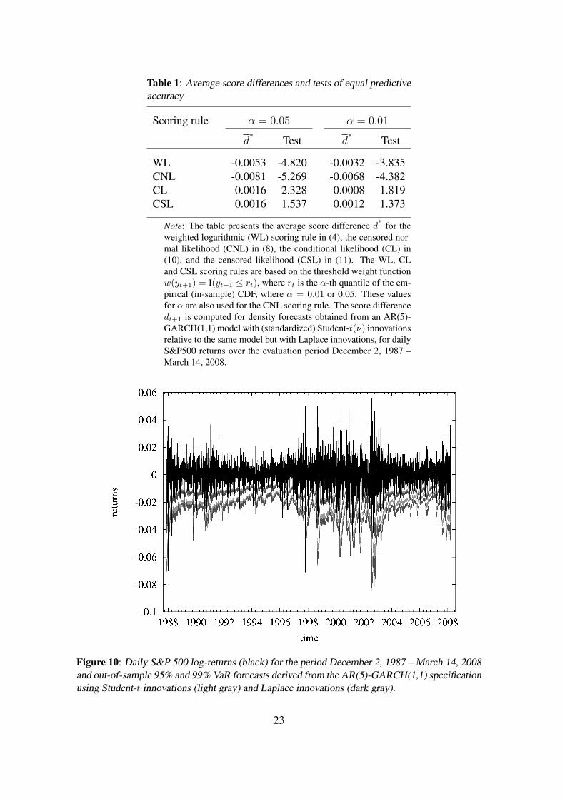
Table 1: Average score differences and tests of equal predictiveaccuracy

Scoring rule α = 0.05 α = 0.01

d∗

Test d∗

Test

WL -0.0053 -4.820 -0.0032 -3.835CNL -0.0081 -5.269 -0.0068 -4.382CL 0.0016 2.328 0.0008 1.819CSL 0.0016 1.537 0.0012 1.373

Note: The table presents the average score difference d∗

for theweighted logarithmic (WL) scoring rule in (4), the censored nor-mal likelihood (CNL) in (8), the conditional likelihood (CL) in(10), and the censored likelihood (CSL) in (11). The WL, CLand CSL scoring rules are based on the threshold weight functionw(yt+1) = I(yt+1 ≤ rt), where rt is the α-th quantile of the em-pirical (in-sample) CDF, where α = 0.01 or 0.05. These valuesfor α are also used for the CNL scoring rule. The score differencedt+1 is computed for density forecasts obtained from an AR(5)-GARCH(1,1) model with (standardized) Student-t(ν) innovationsrelative to the same model but with Laplace innovations, for dailyS&P500 returns over the evaluation period December 2, 1987 –March 14, 2008.

Figure 10: Daily S&P 500 log-returns (black) for the period December 2, 1987 – March 14, 2008and out-of-sample 95% and 99% VaR forecasts derived from the AR(5)-GARCH(1,1) specificationusing Student-t innovations (light gray) and Laplace innovations (dark gray).

23

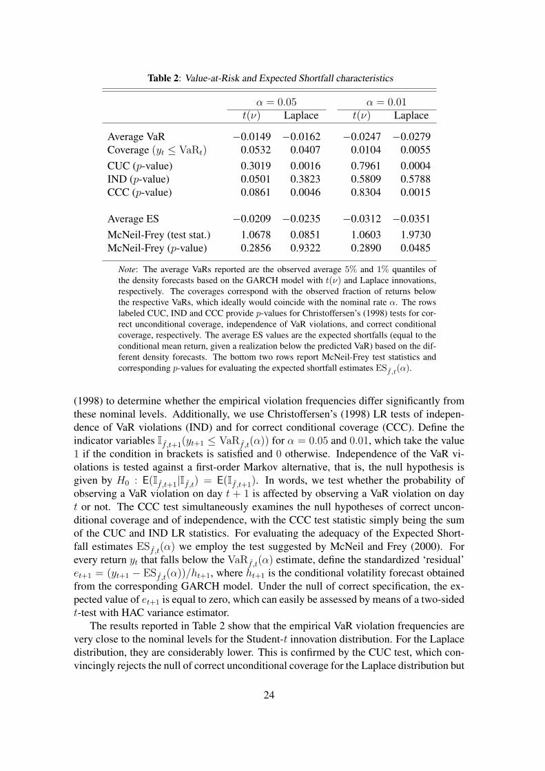
Table 2: Value-at-Risk and Expected Shortfall characteristics

α = 0.05 α = 0.01t(ν) Laplace t(ν) Laplace

Average VaR −0.0149 −0.0162 −0.0247 −0.0279Coverage (yt ≤ VaRt) 0.0532 0.0407 0.0104 0.0055CUC (p-value) 0.3019 0.0016 0.7961 0.0004IND (p-value) 0.0501 0.3823 0.5809 0.5788CCC (p-value) 0.0861 0.0046 0.8304 0.0015

Average ES −0.0209 −0.0235 −0.0312 −0.0351McNeil-Frey (test stat.) 1.0678 0.0851 1.0603 1.9730McNeil-Frey (p-value) 0.2856 0.9322 0.2890 0.0485

Note: The average VaRs reported are the observed average 5% and 1% quantiles ofthe density forecasts based on the GARCH model with t(ν) and Laplace innovations,respectively. The coverages correspond with the observed fraction of returns belowthe respective VaRs, which ideally would coincide with the nominal rate α. The rowslabeled CUC, IND and CCC provide p-values for Christoffersen’s (1998) tests for cor-rect unconditional coverage, independence of VaR violations, and correct conditionalcoverage, respectively. The average ES values are the expected shortfalls (equal to theconditional mean return, given a realization below the predicted VaR) based on the dif-ferent density forecasts. The bottom two rows report McNeil-Frey test statistics andcorresponding p-values for evaluating the expected shortfall estimates ESf ,t(α).

(1998) to determine whether the empirical violation frequencies differ significantly fromthese nominal levels. Additionally, we use Christoffersen’s (1998) LR tests of indepen-dence of VaR violations (IND) and for correct conditional coverage (CCC). Define theindicator variables If ,t+1(yt+1 ≤ VaRf ,t(α)) for α = 0.05 and 0.01, which take the value1 if the condition in brackets is satisfied and 0 otherwise. Independence of the VaR vi-olations is tested against a first-order Markov alternative, that is, the null hypothesis isgiven by H0 : E(If ,t+1|If ,t) = E(If ,t+1). In words, we test whether the probability ofobserving a VaR violation on day t + 1 is affected by observing a VaR violation on dayt or not. The CCC test simultaneously examines the null hypotheses of correct uncon-ditional coverage and of independence, with the CCC test statistic simply being the sumof the CUC and IND LR statistics. For evaluating the adequacy of the Expected Short-fall estimates ESf ,t(α) we employ the test suggested by McNeil and Frey (2000). Forevery return yt that falls below the VaRf ,t(α) estimate, define the standardized ‘residual’et+1 = (yt+1 − ESf ,t(α))/ht+1, where ht+1 is the conditional volatility forecast obtainedfrom the corresponding GARCH model. Under the null of correct specification, the ex-pected value of et+1 is equal to zero, which can easily be assessed by means of a two-sidedt-test with HAC variance estimator.

The results reported in Table 2 show that the empirical VaR violation frequencies arevery close to the nominal levels for the Student-t innovation distribution. For the Laplacedistribution, they are considerably lower. This is confirmed by the CUC test, which con-vincingly rejects the null of correct unconditional coverage for the Laplace distribution but

24

not for the Student-t distribution. The null hypothesis of independence is not rejected inany of the cases at the 5% significance level. Finally, the McNeil and Frey (2000) test doesnot reject the adequacy of the 95% ES estimates for either of the two distributions, but itdoes for the 99% ES estimates based on the Laplace innovation distribution. In sum, theVaR and ES estimates suggest that the Student-t distribution is more appropriate than theLaplace distribution, confirming the density forecast evaluation results obtained with thescoring rules based on partial likelihood. In terms of risk management, using the GARCH-Laplace forecast method would lead to larger estimates of risk than the GARCH-t forecastmethod. This, in turn, could result in suboptimal asset allocation and ‘over-hedging’.

7 ConclusionsIn this paper we have developed scoring rules based on partial likelihood functions forevaluating the predictive ability of competing density forecasts. It was shown that thesescoring rules are particularly useful when the main interest lies in comparing the densityforecasts’ accuracy for a specific region, such as the left tail in financial risk managementapplications. Conventional scoring rules based on KLIC or censored normal likelihoodare not suitable for this purpose. By construction they tend to favor density forecasts withmore probability mass in the region of interest, rendering the tests of equal predictive ac-curacy biased towards such densities. Our novel scoring rules based on partial likelihoodfunctions do not suffer from this problem.

Monte Carlo simulations were used to demonstrate that the conventional scoring rulesmay indeed give rise to spurious rejections due to the possible bias in favor of an incorrectdensity forecast. The simulation results also showed that this phenomenon is virtuallynon-existent for the new scoring rules, and where present, diminishes quickly upon in-creasing the sample size.

In an empirical application to S&P 500 daily returns we investigated the use of thevarious scoring rules for density forecast comparison in the context of financial risk man-agement. It was shown that the scoring rules based on KLIC and censored normal like-lihood functions and the newly proposed partial likelihood scoring rules can lead to theselection of different density forecasts. The density forecasts preferred by the partial like-lihood scoring rules appear to be more appropriate as they were found to result in moreaccurate estimates of Value-at-Risk and Expected Shortfall.

25

ReferencesAmisano, G. and Giacomini, R. (2007). Comparing density forecasts via weighted likeli-

hood ratio tests. Journal of Business and Economic Statistics, 25, 177–190.

Bai, J. (2003). Testing parametric conditional distributions of dynamic models. Reviewof Economics and Statistics, 85, 531–549.

Bai, J. and Ng, S. (2005). Tests for skewness, kurtosis, and normality of time series data.Journal of Business and Economic Statistics, 23, 49–60.

Baillie, R.T. and Bollerslev, T. (1989). The message in daily exchange rates: Aconditional-variance tale. Journal of Business and Economic Statistics, 7, 297–305.

Bao, Y., Lee, T.-H. and Saltoglu, B. (2004). A test for density forecast comparison withapplications to risk management. Working paper 04-08, UC Riverside.

Bao, Y., Lee, T.-H. and Saltoglu, B. (2007). Comparing density forecast models. Journalof Forecasting, 26, 203–225.

Berg, D. and Bakken, H. (2005). A goodness-of-fit test for copulae based on the probabil-ity integral transform. Technical report number SAMBA/41/05, Norwegian ComputingCenter.

Berkowitz, J. (2001). Testing density forecasts, with applications to risk management.Journal of Business and Economic Statistics, 19, 465–474.

Bollerslev, Tim (1987). A conditionally heteroskedastic time series model for speculativeprices and rates of return. The Review of Economics and Statistics, 69, number 3, 542–547.

Breymann, W., Dias, A. and Embrechts, P. (2003). Dependence structures for multivariatehigh-frequency data in finance. Quantitative Finance, 3, 1–14.

Campbell, S.D. and Diebold, F.X. (2005). Weather forecasting for weather derivatives.Journal of the American Statistical Association, 100, 6–16.

Christoffersen, P.F. (1998). Evaluating interval forecasts. International Economic Review,39, 841–862.

Clements, M.P. (2004). Evaluating the Bank of England density forecasts of inflation.Economic Journal, 114, 844–866.

Clements, M.P. (2005). Evaluating Econometric Forecasts of Economic and FinancialVariables. New York: Palgrave-Macmillan.

Clements, M.P. and Smith, J. (2000). Evaluating the forecast densities of linear andnonlinear models: Applications to output growth and inflation. Journal of Forecasting,19, 255–276.

26

Clements, M.P. and Smith, J. (2002). Evaluating multivariate forecast densities: A com-parison of two approaches. International Journal of Forecasting, 18, 397–407.

Corradi, V. and Swanson, N.R. (2005). A test for comparing multiple misspecified con-ditional interval models. Econometric Theory, 21, 991–1016.

Corradi, V. and Swanson, N.R. (2006a). Bootstrap conditional distribution tests in thepresence of dynamic misspecifation. Journal of Econometrics, 133, 779–806.

Corradi, V. and Swanson, N.R. (2006b). Predictive density and conditional confidenceinterval accuracy tests. Journal of Econometrics, 135, 187–228.

Corradi, V. and Swanson, N.R. (2006c). Predictive density evaluation. In Handbook ofEconomic Forecasting, Volume 1 (eds G. Elliott, C.W.J. Granger and A. Timmermann),pp. 197–284. Amsterdam: Elsevier.

Cox, D.R. (1975). Partial likelihood. Biometrika, 62, 269–276.

Diebold, F.X., Gunther, T.A. and Tay, A.S. (1998). Evaluating density forecasts withapplications to financial risk management. International Economic Review, 39, 863–883.

Diebold, F.X., Hahn, J. and Tay, A.S. (1999). Multivariate density forecast evaluation andcalibration in financial risk management: high-frequency returns on foreign exchange.Review of Economics and Statistics, 81, 661–673.

Diebold, F.X. and Lopez, J.A. (1996). Forecast evaluation and combination. In Handbookof Statistics, Vol. 14 (eds G.S. Maddala and C.R. Rao), pp. 241–268. Amsterdam:North-Holland.

Diebold, F.X. and Mariano, R.S. (1995). Comparing predictive accuracy. Journal ofBusiness and Economic Statistics, 13, 253–263.

Diebold, F.X., Tay, A.S. and Wallis, K.D. (1998). Evaluating density forecasts of inflation:The survey of professional forecasters. In Cointegration, Causality, and Forecasting:A Festschrift in Honor of C.W.J. Granger (eds R.F. Engle and H. White), pp. 76–90.Oxford: Oxford University Press.

Dowd, K. (2005). Measuring Market Risk, 2 edn. Chicester: John Wiley & Sons.

Egorov, A.V., Hong, Y. and Li, H. (2006). Validating forecasts of the joint probabilitydensity of bond yields: Can affine models beat random walk? Journal of Econometrics,135, 255–284.

Franses, P.H. and van Dijk, D. (2003). Selecting a nonlinear time series model usingweighted tests of equal forecast accuracy. Oxford Bulletin of Economics and Statistics,65, 727–744.

27

Garratt, A., Lee, K., Pesaran, M.H. and Shin, Y. (2003). Forecast uncertainties in macroe-conomic modelling: An application to the UK economy. Journal of the AmericanStatistical Association, 98, 829–838.

Giacomini, R. and White, H. (2006). Tests of conditional predictive ability. Econometrica,74, 1545–1578.

Granger, C.W.J. and Ding, Z. (1995). Some properties of absolute return, an alternativemeasure of risk. Annales d’Economie et de Statistique, 40, 67–91.

Granger, C.W.J. and Pesaran, M.H. (2000). Economic and statistical measures of forecastaccuracy. Journal of Forecasting, 19, 537–560.

Guidolin, M. and Timmermann, A. (2006). Term structure of risk under alternativeeconometric specifications. Journal of Econometrics, 131, 285–308.

Guidolin, M. and Timmermann, A. (2007). Asset allocation under multivariate regimeswitching. Journal of Economic Dynamics and Control, 31, 3503–3544.

Hall, S.G. and Mitchell, J. (2007). Combining density forecasts. International Journal ofForecasting, 23, 1–13.

Hong, Y. and Li, H. (2005). Nonparametric specification testing for continuous-timemodels with applications to term structure of interest rates. Review of Financial Studies,18, 37–84.

Hong, Y., Li, H. and Zhao, F. (2004). Out-of-sample performance of discrete-time spotinterest rate models. Journal of Business and Economic Statistics, 22, 457–473.

Lahiri, K. and Wang, J.G. (2007). Evaluating probability forecasts for GDP declines.Working paper, University of Albany - SUNY.

Li, F. and Tkacz, G. (2006). A consistent bootstrap test for conditional density functionswith time-series data. Journal of Econometrics, 133, 863–886.

McNeil, A.J. and Frey, R. (2000). Estimation of tail-related risk measures for het-eroscedastic financial time series: an extreme value approach. Journal of EmpiricalFinance, 7, 271–300.

McNeil, A.J., Frey, R. and Embrechts, P. (2005). Quantitative Risk Management: Con-cepts, Techniques, and Tools. Princeton: Princeton University Press.

Mitchell, J. and Hall, S.G. (2005). Evaluating, comparing and combining density forecastsusing the KLIC with an application to the Bank of England and NIESR ‘fan’ charts ofinflation. Oxford Bulletin of Economics and Statistics, 67, 995–1033.

Mittnik, S., Paolella, M.S. and Rachev, S.T. (1998). Unconditional and conditional distri-butional models for the Nikkei index. Asia-Pacific Financial Markets, 5, 99–128.

28

Perez-Quiros, G. and Timmermann, A. (2001). Business cycle asymmetries in stockreturns: Evidence from higher order moments and conditional densities. Journal ofEconometrics, 103, 259–306.

Rapach, D.E. and Wohar, M.E. (2006). The out-of-sample forecasting performance ofnonlinear models of real exchange rate behavior. International Journal of Forecasting,22, 341–361.

Rosenblatt, M. (1952). Remarks on a multivariate transformation. Annals of MathematicalStatistics, 23, 470–472.

Sarno, L. and Valente, G. (2004). Comparing the accuracy of density forecasts fromcompeting models. Journal of Forecasting, 23, 541–557.

Sarno, L. and Valente, G. (2005). Empirical exchange rate models and currency risk:Some evidence from density forecasts. Journal of International Money and Finance,24, 363–385.

Taylor, J.W. and Buizza, R. (2006). Density forecasting for weather derivative pricing.International Journal of Forecasting, 22, 29–42.

Tobin, J. (1958). Estimation of relationships for limited dependent variables. Economet-rica, 26, 24–36.

White, H. (2000). A reality check for data snooping. Econometrica, 68, 1097–1126.

29