Particle-based Viscoelastic Fluid Simulation · S. Clavet, P. Beaudoin, and P. Poulin / Particle-based Viscoelastic Fluid Simulation allows for direct specication of well-dened physical

Eurographics/ACM SIGGRAPH Symposium on Computer Animation (2005)K. Anjyo, P. Faloutsos (Editors)

Particle-based Viscoelastic Fluid Simulation

Simon Clavet, Philippe Beaudoin, and Pierre Poulin †

LIGUM, Dept. IRO, Université de Montréal

Abstract

We present a new particle-based method for viscoelastic fluid simulation. We achieve realistic small-scale behaviorof substances such as paint or mud as they splash on moving objects. Incompressibility and particle anti-clusteringare enforced with a double density relaxation procedure which updates particle positions according to two oppos-ing pressure terms. From this process surface tension effects emerge, enabling drop and filament formation. Elasticand non-linear plastic effects are obtained by adding springs with varying rest length between particles. We alsoextend the technique to handle interaction between fluid and dynamic objects. Various simulation scenarios arepresented including rain drops, fountains, clay manipulation, and floating objects. The method is robust and stable,and can animate splashing behavior at interactive framerates.

Categories and Subject Descriptors (according to ACM CCS): I.3.5 [Computer Graphics]: Computational Geometryand Object Modeling – Physically Based Modeling; I.3.7 [Computer Graphics]: Three-Dimensional Graphics andRealism – Animation and Virtual Reality

1. Introduction

The field of computational fluid dynamics has introducedmany different algorithms to simulate the complex behav-ior of fluids. Since liquids and gases play an important rolein everyday life, several fluid simulation methods have beensuccessfully used for computer graphics applications.

Two main categories of simulation methods exist: Eule-rian grids and Lagrangian particles. Eulerian methods dis-cretize the problem using a subdivision of the spatial do-main and control fluid flow in each cell. Such techniqueshave been able to achieve among the most realistic simu-lations of liquid types ranging from simple flows to highlyviscous fluids, with plastic and elastic behaviors. They easilyenforce the incompressibility condition, but do not guaranteemass conservation for small features.

Lagrangian methods discretize the fluid mass using par-ticles. By directly tracking chunks of matter as they travelthrough space, particle methods trivially guarantee massconservation and provide a conceptually simple and versa-tile simulation framework.

† email: clavetsi | beaudoin | [email protected]

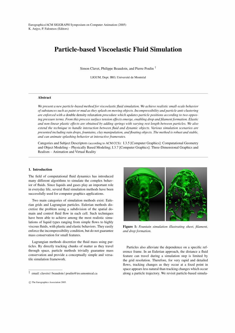
Figure 1: Fountain simulation illustrating sheet, filament,and drop formation.

Particles also alleviate the dependence on a specific ref-erence frame. In an Eulerian approach, the distance a fluidfeature can travel during a simulation step is limited bythe grid resolution. Therefore, for very rapid and detailedflows, tracking changes as they occur at a fixed point inspace appears less natural than tracking changes which occuralong a particle trajectory. We revisit particle-based simula-

c© The Eurographics Association 2005.

S. Clavet, P. Beaudoin, and P. Poulin / Particle-based Viscoelastic Fluid Simulation

tion and propose extensions and modifications that increasetheir flexibility and robustness. Our formulation is simpleand intuitive, and it can be implemented within days.

An important disadvantage of particle simulations is thedifficulty to represent a smooth surface with particles. Ro-bustly handling surface tension effects for small features isalso recognized as a difficult task. Surface tension forces ex-ist at the surface of the fluid, and depend on its curvature.The problem comes from the fact that particle simulationsavoid modeling the surface explicitly, and thus robustly com-puting its curvature can be cumbersome.

We propose a novel procedure for incompressibility andparticle anti-clustering. We call this procedure double den-sity relaxation. Loosely speaking, double density relaxationcomputes two different particle densities: one quantifyingthe number of neighbors, and another quantifying the num-ber of close neighbors. The force between two particles de-pends on these two context-dependent measures, instead ofdepending only on the distance between them. Liquids an-imated with this method display a smooth particle surface,and surface tension effects such as those shown in Figure 1emerge naturally. No curvature has to be evaluated, and theprocedure is robust even in presence of small surface details.

Numerical instabilities are often an issue with anyphysically-based simulations, requiring the use of pro-hibitively small timesteps. We use a conceptually intuitiveprediction-relaxation scheme that remains stable even forlarge timesteps and fast splashing effects.

We also present a simple method to simulate viscoelas-tic substances by insertion and removal of springs betweenpairs of particles. Various material behaviors can be obtainedwith simple spring rest length update rules. The intuitive pa-rameters governing such a scheme, combined with our fastsimulation, allow an artist to interactively experiment withthe fluid properties to obtain the desired results.

Finally, we describe a simple way to integrate the fluidsolver with a rigid-body simulator, enabling two-way cou-pling between liquids and objects. We also propose a simplesolution to the stickiness of liquids on objects.

2. Previous Work

2.1. Eulerian Simulation

Grid-based methods have been quite popular for computergraphics applications. Foster and Metaxas [FM96, FM97]were the first to propose solving the full 3D Navier-Stokesequations on a regular grid in order to re-create the visualproperties of a dynamic fluid. Stam [Sta99] produced dy-namic gases using a semi-Lagrangian integration schemethat achieves unconditional stability at the expense of ar-tificial viscosity and rotational damping. Foster and Fed-kiw [FF01] extended the technique to liquids, tracking thesurface using both a level-set method and particles inside

the liquid. Enright et al. [EMF02] added particles outsidethe fluid volume to improve surface tracking. They also pro-posed an extrapolation technique to assign velocities to aircells just outside the liquid surface, resulting in a smoothersurface motion on a coarse grid.

A number of researchers have developed methods formodeling highly viscous or viscoelastic fluids. Carlson etal. [CMHT02] developed an Eulerian solver for very highviscosity liquids and were able to simulate melting objects.Fluids simulated by Goktekin et al. [GBO04] exhibit notonly viscous but also elastic and plastic behaviors by inte-grating and advecting strain-rate throughout the fluid.

2.2. Lagrangian Simulation

Smoothed particle hydrodynamics (SPH) is an alternativeapproach, first developed by Lucy [Luc77] and by Gingoldand Monaghan [GM77], to tackle astrophysical problems. InSPH, space is non-uniformly sampled using particles. Theseparticles maintain various field properties, such as mass den-sity or velocity, and are tracked during the simulation. Thefield quantities can be evaluated anywhere in space using ra-dially symmetric smoothing kernels.

Reeves [Ree83] introduced particle systems to computergraphics. They quickly became a popular tool for portrayingvarious effects such as fire or waterfalls. Miller and Pearce[MP89] borrowed ideas from molecular dynamics to add ba-sic particle interactions, resulting in limited simulations ofliquids and melting solids. Terzopoulos et al. [TPF89] mod-eled melting thermoelastic materials using particles that ap-ply various forces to their neighbors. In a solid material,the particles are connected with springs, which weaken andeventually disappear as the material melts. This model doesnot handle plasticity.

Desbrun and Gascuel [DG96] applied SPH concepts tocomputer graphics in order to simulate highly deformablebodies. Recently, Müller et al. [MCG03] implemented in-teractive liquid simulation and rendering using SPH. Theysimulate surface tension using ideas from Morris [Mor00],implicitly defining an interface with the particles and apply-ing a force proportional to curvature, computed as the diver-gence of the normal field. For surface features representedby a small number of particles, such curvature evaluationcan cause numerical problems.

Premože et al. [PTB∗03] also obtained realistic lookingfluids using a Lagrangian method. They solve the Navier-Stokes equations using the Moving-Particle Semi-Implicit(MPS) method [KO96], which ensures a greater level of in-compressibility than standard SPH.

Müller et al. [MKN∗04] proposed a particle-basedmethod for animating volumetric objects with material prop-erties ranging from stiff elastic to highly plastic. Their tech-nique is derived from continuum mechanics and therefore



allows for direct specification of well-defined physical prop-erties. Although they do not try to simulate a flowing liquid,they obtain very realistic results for the material types sup-ported.

Steele et al. [SCED04] presented a particle-based methodfor simulating viscous liquids. They define the adhesionproperties of different types of particles using generaldistance-dependent forces between particles. Their iterativerelaxation scheme to conserve volume is similar to ours, butthe linear density kernel and the hard anti-penetration con-straints limit their method to highly viscous fluids.

3. Simulation Step

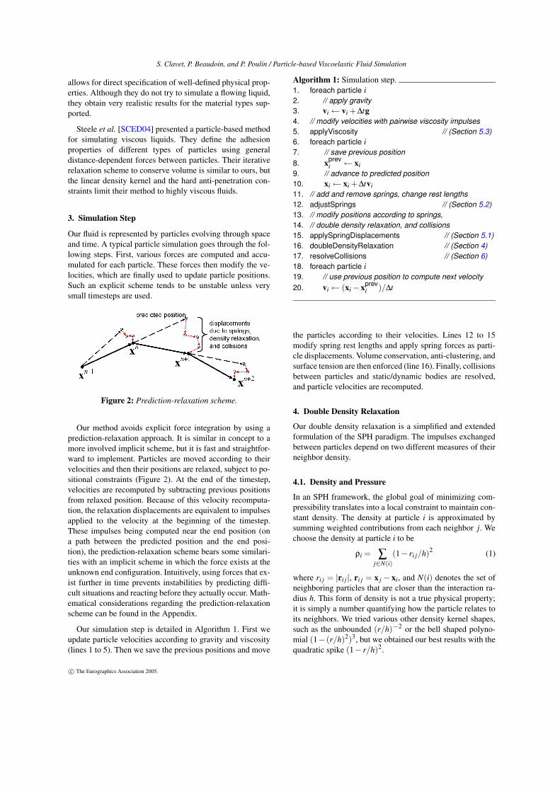
Our fluid is represented by particles evolving through spaceand time. A typical particle simulation goes through the fol-lowing steps. First, various forces are computed and accu-mulated for each particle. These forces then modify the ve-locities, which are finally used to update particle positions.Such an explicit scheme tends to be unstable unless verysmall timesteps are used.

Figure 2: Prediction-relaxation scheme.

Our method avoids explicit force integration by using aprediction-relaxation approach. It is similar in concept to amore involved implicit scheme, but it is fast and straightfor-ward to implement. Particles are moved according to theirvelocities and then their positions are relaxed, subject to po-sitional constraints (Figure 2). At the end of the timestep,velocities are recomputed by subtracting previous positionsfrom relaxed position. Because of this velocity recomputa-tion, the relaxation displacements are equivalent to impulsesapplied to the velocity at the beginning of the timestep.These impulses being computed near the end position (ona path between the predicted position and the end posi-tion), the prediction-relaxation scheme bears some similari-ties with an implicit scheme in which the force exists at theunknown end configuration. Intuitively, using forces that ex-ist further in time prevents instabilities by predicting diffi-cult situations and reacting before they actually occur. Math-ematical considerations regarding the prediction-relaxationscheme can be found in the Appendix.

Our simulation step is detailed in Algorithm 1. First weupdate particle velocities according to gravity and viscosity(lines 1 to 5). Then we save the previous positions and move

Algorithm 1: Simulation step.1. foreach particle i2. // apply gravity3. vi← vi +∆tg4. // modify velocities with pairwise viscosity impulses5. applyViscosity // (Section 5.3)6. foreach particle i7. // save previous position8. xprev

i ← xi9. // advance to predicted position10. xi← xi +∆tvi11. // add and remove springs, change rest lengths12. adjustSprings // (Section 5.2)13. // modify positions according to springs,14. // double density relaxation, and collisions15. applySpringDisplacements // (Section 5.1)16. doubleDensityRelaxation // (Section 4)17. resolveCollisions // (Section 6)18. foreach particle i19. // use previous position to compute next velocity20. vi← (xi−xprev

i )/∆t

the particles according to their velocities. Lines 12 to 15modify spring rest lengths and apply spring forces as parti-cle displacements. Volume conservation, anti-clustering, andsurface tension are then enforced (line 16). Finally, collisionsbetween particles and static/dynamic bodies are resolved,and particle velocities are recomputed.

4. Double Density Relaxation

Our double density relaxation is a simplified and extendedformulation of the SPH paradigm. The impulses exchangedbetween particles depend on two different measures of theirneighbor density.

4.1. Density and Pressure

In an SPH framework, the global goal of minimizing com-pressibility translates into a local constraint to maintain con-stant density. The density at particle i is approximated bysumming weighted contributions from each neighbor j. Wechoose the density at particle i to be

ρi = ∑j∈N(i)

(1− ri j/h)2 (1)

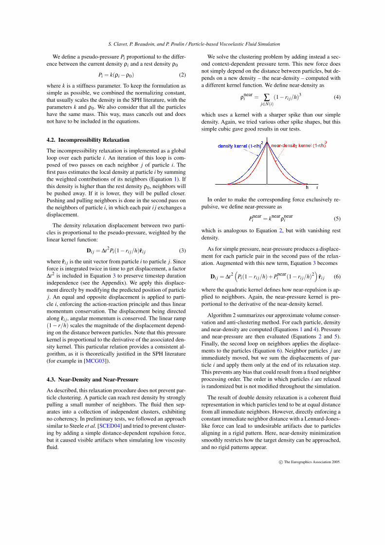
where ri j = |ri j|, ri j = x j − xi, and N(i) denotes the set ofneighboring particles that are closer than the interaction ra-dius h. This form of density is not a true physical property;it is simply a number quantifying how the particle relates toits neighbors. We tried various other density kernel shapes,such as the unbounded (r/h)−2 or the bell shaped polyno-mial (1− (r/h)2)3, but we obtained our best results with thequadratic spike (1− r/h)2.



We define a pseudo-pressure Pi proportional to the differ-ence between the current density ρi and a rest density ρ0

Pi = k(ρi−ρ0) (2)

where k is a stiffness parameter. To keep the formulation assimple as possible, we combined the normalizing constant,that usually scales the density in the SPH literature, with theparameters k and ρ0. We also consider that all the particleshave the same mass. This way, mass cancels out and doesnot have to be included in the equations.

4.2. Incompressibility Relaxation

The incompressibility relaxation is implemented as a globalloop over each particle i. An iteration of this loop is com-posed of two passes on each neighbor j of particle i. Thefirst pass estimates the local density at particle i by summingthe weighted contributions of its neighbors (Equation 1). Ifthis density is higher than the rest density ρ0, neighbors willbe pushed away. If it is lower, they will be pulled closer.Pushing and pulling neighbors is done in the second pass onthe neighbors of particle i, in which each pair i j exchanges adisplacement.

The density relaxation displacement between two parti-cles is proportional to the pseudo-pressure, weighted by thelinear kernel function:

Di j = ∆t2Pi(1− ri j/h)r̂i j (3)

where r̂i j is the unit vector from particle i to particle j. Sinceforce is integrated twice in time to get displacement, a factor∆t2 is included in Equation 3 to preserve timestep durationindependence (see the Appendix). We apply this displace-ment directly by modifying the predicted position of particlej. An equal and opposite displacement is applied to parti-cle i, enforcing the action-reaction principle and thus linearmomentum conservation. The displacement being directedalong r̂i j , angular momentum is conserved. The linear ramp(1− r/h) scales the magnitude of the displacement depend-ing on the distance between particles. Note that this pressurekernel is proportional to the derivative of the associated den-sity kernel. This particular relation provides a consistent al-gorithm, as it is theoretically justified in the SPH literature(for example in [MCG03]).

4.3. Near-Density and Near-Pressure

As described, this relaxation procedure does not prevent par-ticle clustering. A particle can reach rest density by stronglypulling a small number of neighbors. The fluid then sep-arates into a collection of independent clusters, exhibitingno coherency. In preliminary tests, we followed an approachsimilar to Steele et al. [SCED04] and tried to prevent cluster-ing by adding a simple distance-dependent repulsion force,but it caused visible artifacts when simulating low viscosityfluid.

We solve the clustering problem by adding instead a sec-ond context-dependent pressure term. This new force doesnot simply depend on the distance between particles, but de-pends on a new density – the near-density – computed witha different kernel function. We define near-density as

ρneari = ∑

j∈N(i)(1− ri j/h)3 (4)

which uses a kernel with a sharper spike than our simpledensity. Again, we tried various other spike shapes, but thissimple cubic gave good results in our tests.

In order to make the corresponding force exclusively re-pulsive, we define near-pressure as

Pneari = knearρnear

i (5)

which is analogous to Equation 2, but with vanishing restdensity.

As for simple pressure, near-pressure produces a displace-ment for each particle pair in the second pass of the relax-ation. Augmented with this new term, Equation 3 becomes

Di j = ∆t2(

Pi(1− ri j/h)+Pneari (1− ri j/h)2

)

r̂i j (6)

where the quadratic kernel defines how near-repulsion is ap-plied to neighbors. Again, the near-pressure kernel is pro-portional to the derivative of the near-density kernel.

Algorithm 2 summarizes our approximate volume conser-vation and anti-clustering method. For each particle, densityand near-density are computed (Equations 1 and 4). Pressureand near-pressure are then evaluated (Equations 2 and 5).Finally, the second loop on neighbors applies the displace-ments to the particles (Equation 6). Neighbor particles j areimmediately moved, but we sum the displacements of par-ticle i and apply them only at the end of its relaxation step.This prevents any bias that could result from a fixed neighborprocessing order. The order in which particles i are relaxedis randomized but is not modified throughout the simulation.

The result of double density relaxation is a coherent fluidrepresentation in which particles tend to be at equal distancefrom all immediate neighbors. However, directly enforcing aconstant immediate neighbor distance with a Lennard-Jones-like force can lead to undesirable artifacts due to particlesaligning in a rigid pattern. Here, near-density minimizationsmoothly restricts how the target density can be approached,and no rigid patterns appear.



Algorithm 2: Double density relaxation.1. foreach particle i2. ρ← 03. ρnear← 04. // compute density and near-density5. foreach particle j ∈ neighbors( i )6. q← ri j/h7. if q < 18. ρ← ρ+(1−q)2

9. ρnear← ρnear +(1−q)3

10. // compute pressure and near-pressure11. P← k(ρ−ρ0)12. Pnear← knearρnear

13. dx← 014. foreach particle j ∈ neighbors( i )15. q← ri j/h16. if q < 117. // apply displacements18. D← ∆t2(P(1−q)+Pnear(1−q)2)r̂i j19. x j← x j +D/220. dx← dx−D/221. xi← xi +dx

4.4. Surface Tension

We observed that besides reducing particle clustering, ourmethod provides another important fluid behavior: surfacetension effects. As illustrated in Figure 3 and in the accom-panying video [VID], particles group into structures such assheets, filaments, and drops.

Figure 3: Oscillating drop.

Surface tension is physically caused by attraction betweenmolecules. Inside the fluid, this attraction cancels out, but formolecules near the surface, asymmetry in neighbor distribu-tion results in a non-zero net force towards the fluid. Further-more, this asymmetry changes depending on surface curva-ture. In view of these physical considerations, surface ten-sion is usually considered to be an external force oriented to-wards the negative surface normal and with magnitude pro-portional to the surface curvature.

We can visualize how the combined effect of pressureand near-pressure can produce surface tension. Suppose thatdensity at a particle position is smaller than rest density.Neighboring particles will be pulled by pressure with animpulse proportional to the linear kernel, and then pushedby near-pressure with an impulse proportional to the sharp-spiked quadratic kernel. Neighbors that are further away

will tend to move more since they are not affected muchby near-pressure. The smooth repulsion of the nearest parti-cles causes an indirect long-distance attraction. This context-aware attraction leads to smooth and stable particle struc-tures.

5. Viscoelasticity

Viscoelastic behavior is introduced in our model throughthree sub-processes: elasticity, plasticity, and viscosity. Elas-ticity is obtained by inserting springs between particles, plas-ticity comes from the modification of the spring rest lengths,and viscosity is introduced by exchanging radial impulsesdetermined by particle velocity differences.

5.1. Elasticity

To simulate elastic behavior, we add springs between pairsof neighboring particles. Springs create displacements on thetwo attached particles. The displacement magnitude is pro-portional to L− r, where r is the distance between the parti-cles and L is the spring rest length. It is also scaled with thefactor 1−L/h, which gradually reduces to zero the force ex-erted by long springs. The process is detailed in Algorithm 3.

Algorithm 3: Spring displacements.1. foreach spring i j2. D← ∆t2kspring(1−Li j/h)(Li j− ri j)r̂i j3. xi← xi−D/24. x j← x j +D/2

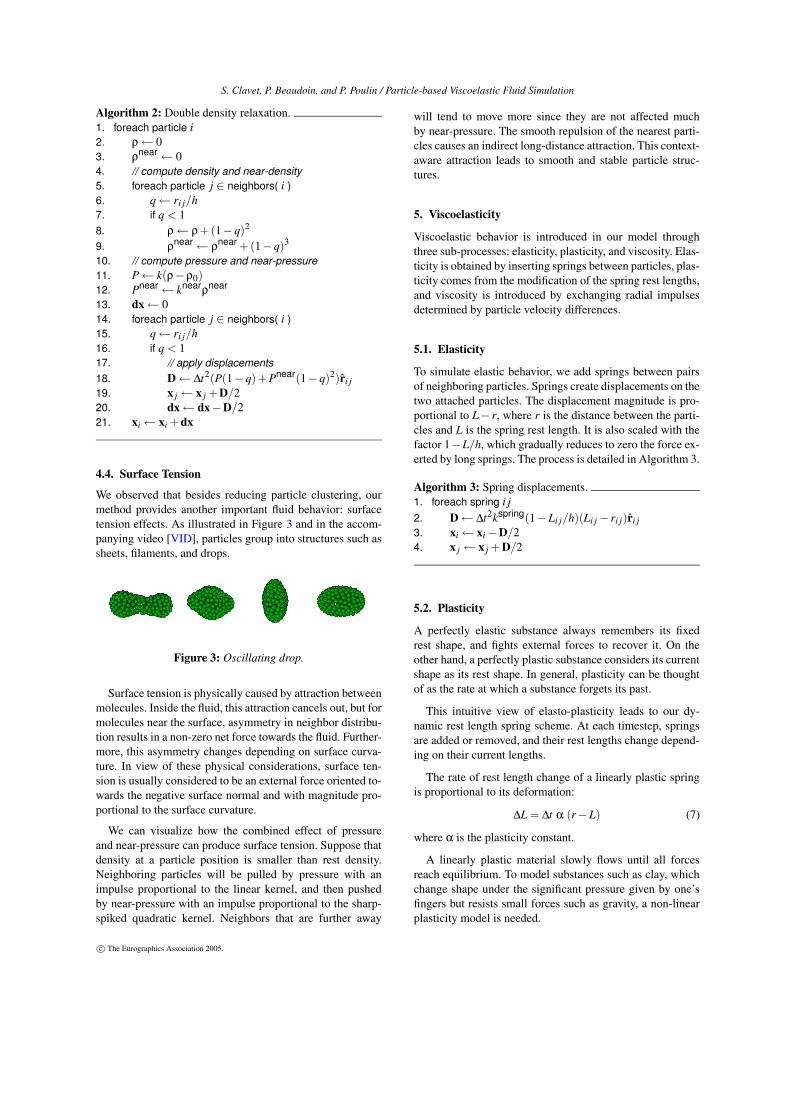
5.2. Plasticity

A perfectly elastic substance always remembers its fixedrest shape, and fights external forces to recover it. On theother hand, a perfectly plastic substance considers its currentshape as its rest shape. In general, plasticity can be thoughtof as the rate at which a substance forgets its past.

This intuitive view of elasto-plasticity leads to our dy-namic rest length spring scheme. At each timestep, springsare added or removed, and their rest lengths change depend-ing on their current lengths.

The rate of rest length change of a linearly plastic springis proportional to its deformation:

∆L = ∆t α (r−L) (7)

where α is the plasticity constant.

A linearly plastic material slowly flows until all forcesreach equilibrium. To model substances such as clay, whichchange shape under the significant pressure given by one’sfingers but resists small forces such as gravity, a non-linearplasticity model is needed.



Algorithm 4: Spring adjustment.1. foreach neighbor pair i j, (i < j)2. q← ri j/h3. if q < 14. if there is no spring i j5. add spring i j with rest length h6. // tolerable deformation = yield ratio * rest length7. d← γ Li j8. if ri j > L+d // stretch9. Li j← Li j +∆t α (ri j−L−d)10. else if ri j < L−d // compress11. Li j← Li j−∆t α (L−d− ri j)12. foreach spring i j13. if Li j > h14. remove spring i j

Our plastic spring model is inspired by the von Mises con-dition [Fun65], which states that plastic flow should occuronly if the deformation is large enough. Translated into thespring system, this means that L should be changed only if|r−L| is larger than some fraction of L (Figure 4). This frac-tion is specified by the yield ratio, denoted γ, for which wetypically choose a value between 0 and 0.2 . The rest lengthincrement can then be written

∆L = ∆t α sign(r−L) max(0, |r−L|− γL) (8)

which becomes identical to Equation 7 when γ = 0.

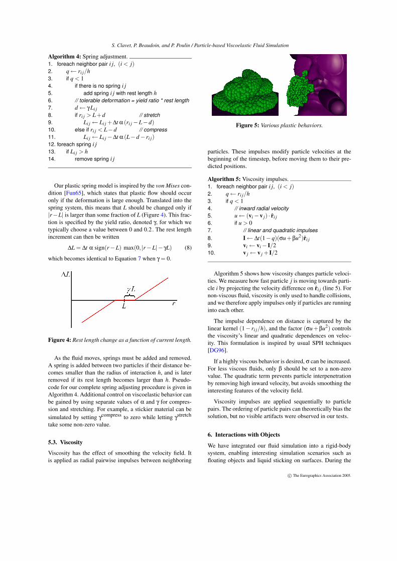
Figure 4: Rest length change as a function of current length.

As the fluid moves, springs must be added and removed.A spring is added between two particles if their distance be-comes smaller than the radius of interaction h, and is laterremoved if its rest length becomes larger than h. Pseudo-code for our complete spring adjusting procedure is given inAlgorithm 4. Additional control on viscoelastic behavior canbe gained by using separate values of α and γ for compres-sion and stretching. For example, a stickier material can besimulated by setting γcompress to zero while letting γstretch

take some non-zero value.

5.3. Viscosity

Viscosity has the effect of smoothing the velocity field. Itis applied as radial pairwise impulses between neighboring

Figure 5: Various plastic behaviors.

particles. These impulses modify particle velocities at thebeginning of the timestep, before moving them to their pre-dicted positions.

Algorithm 5: Viscosity impulses.1. foreach neighbor pair i j, (i < j)2. q← ri j/h3. if q < 14. // inward radial velocity5. u← (vi−v j) · r̂i j6. if u > 07. // linear and quadratic impulses8. I← ∆t(1−q)(σu+βu2)r̂i j9. vi← vi− I/210. v j← v j + I/2

Algorithm 5 shows how viscosity changes particle veloci-ties. We measure how fast particle j is moving towards parti-cle i by projecting the velocity difference on r̂i j (line 5). Fornon-viscous fluid, viscosity is only used to handle collisions,and we therefore apply impulses only if particles are runninginto each other.

The impulse dependence on distance is captured by thelinear kernel (1− ri j/h), and the factor (σu + βu2) controlsthe viscosity’s linear and quadratic dependences on veloc-ity. This formulation is inspired by usual SPH techniques[DG96].

If a highly viscous behavior is desired, σ can be increased.For less viscous fluids, only β should be set to a non-zerovalue. The quadratic term prevents particle interpenetrationby removing high inward velocity, but avoids smoothing theinteresting features of the velocity field.

Viscosity impulses are applied sequentially to particlepairs. The ordering of particle pairs can theoretically bias thesolution, but no visible artifacts were observed in our tests.

6. Interactions with Objects

We have integrated our fluid simulation into a rigid-bodysystem, enabling interesting simulation scenarios such asfloating objects and liquid sticking on surfaces. During the



collision stage, the fluid is considered to be an assembly ofrigid spheres exchanging impulses with surrounding objects.

6.1. Collisions

For each object, a signed distance field is sampled and storedin a grid structure. For each particle we obtain the interpo-lated distance value d. A collision is identified when d issmaller than the particle collision radius R. For the collid-ing particle we obtain the object normal n̂ using the distancefield gradient.

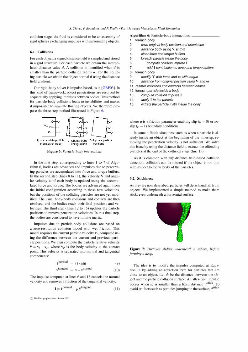
Our rigid-body solver is impulse-based, as in [GBF03]. Inthis kind of framework, object penetrations are resolved bysequentially applying impulses between bodies. This methodfor particle-body collisions leads to instabilities and makesit impossible to simulate floating objects. We therefore pro-pose the three step method illustrated in Figure 6.

Figure 6: Particle-body interactions.

In the first step, corresponding to lines 1 to 7 of Algo-rithm 6, bodies are advanced and impulses due to penetrat-ing particles are accumulated into force and torque buffers.In the second step (lines 8 to 11), the velocity V and angu-lar velocity ω of each body is updated using the accumu-lated force and torque. The bodies are advanced again fromthe initial configuration according to these new velocities,but the positions of the colliding particles are not yet mod-ified. The usual body-body collisions and contacts are thenresolved, and the bodies reach their final positions and ve-locities. The third step (lines 12 to 15) updates the particlepositions to remove penetration velocities. In this final step,the bodies are considered to have infinite inertia.

Impulses due to particle-body collisions are based ona zero-restitution collision model with wet friction. Thismodel requires the current particle velocity vi, computed us-ing the difference between the current and previous parti-cle positions. We then compute the particle relative velocityv̄ = vi − vp, where vp is the body velocity at the contactpoint. This velocity is separated into normal and tangentialcomponents:

v̄normal = (v̄ · n̂)n̂ (9)

v̄tangent = v̄− v̄normal. (10)

The impulse computed at lines 6 and 13 cancels the normalvelocity and removes a fraction of the tangential velocity:

I = v̄normal−µ v̄tangent (11)

Algorithm 6: Particle-body interactions.1. foreach body2. save original body position and orientation3. advance body using V and ω4. clear force and torque buffers5. foreach particle inside the body6. compute collision impulse I7. add I contribution to force and torque buffers8. foreach body9. modify V with force and ω with torque10. advance from original position using V and ω11. resolve collisions and contacts between bodies12. foreach particle inside a body13. compute collision impulse I14. apply I to the particle15. extract the particle if still inside the body

where µ is a friction parameter enabling slip (µ = 0) or no-slip (µ = 1) boundary conditions.

In some difficult situations, such as when a particle is al-ready inside an object at the beginning of the timestep, re-moving the penetration velocity is not sufficient. We solvethis issue by using the distance field to extract the offendingparticles at the end of the collision stage (line 15).

As it is common with any distance field-based collisiondetection, collisions can be missed if the object is too thinwith respect to the velocity of the particles.

6.2. Stickiness

As they are now described, particles will detach and fall fromobjects. We implemented a simple method to make themstick, even underneath a horizontal surface.

Figure 7: Particles sliding underneath a sphere, beforeforming a drop.

The idea is to modify the impulse computed at Equa-tion 11 by adding an attraction term for particles that areclose to an object. Let di be the distance between the ob-ject and the particle collision surface. An attraction impulseoccurs when di is smaller than a fixed distance dstick. Toavoid artifacts such as particles jumping to the surface, dstick



should stay small enough with respect to the particle inter-action range h. We use the following formulation:

Istick =−∆t kstickdi

(

1−di

dstick

)

n̂ (12)

which is maximal at distance dstick/2. Lines 5 and 12 ofAlgorithm 7 must now consider all particles in the attractionrange.

7. Implementation and Results

7.1. Neighbor Search

Finding all particles that are within the interaction radius ofa particle is a frequent task in any particle-based method.Since the interaction radius h is constant and identical foreach particle, it makes sense to use a simple regular spa-tial hashing grid with cube size h. Each cube stores a listof enclosed particles, which is updated each time a parti-cle moves from one cube to another. All neighbors residein the particle’s cube and its 26 neighboring cubes. Further-more, we avoid using a fixed cube lattice by only instanti-ating cubes that contain particles. The cubes are stored in ahash table, indexed with their 3D index. The animation sce-nario can thus take place in a virtually infinite domain, andno information on the future location of the fluid is needed atthe beginning of the simulation. This spatial hashing methodis similar to Teschner et al. [THM∗03].

7.2. Rendering

For fast previsualization, particles are simply rendered aspolygonized spheres. High quality rendering uses a surfacemesh extracted with the marching cube algorithm [LC87].

The marching cube extracts an isosurface of a scalar func-tion defined by the particles. We use the function

φ(x) =

(

∑j(1− r/h)2

)12

(13)

where r = |x−x j|. The square root ensures that the functionbehaves like a distance function, i.e., has an almost constantslope around the extracted isosurface. This is important formoving isosurfaces because the location of the surface in acube is linearly interpolated. If the function had a changingslope around the isovalue, temporal artifacts would appear asparticles move. Simply using a sum of cones could achievethis goal, but the result would not be smooth enough.

As in the case of neighbor search, the cube grid used forisosurface extraction is sparse and dynamic. The cube sizehsurface is independent from the particle interaction radius h,and is typically smaller if a smooth surface mesh is desired.A spatial hash table is used to store the non-zero grid pointsas particles add their contributions to the implicit function.

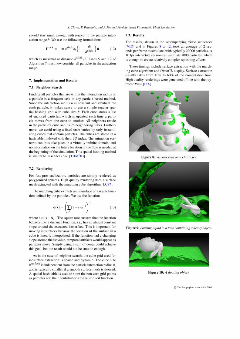
7.3. Results

The results, shown in the accompanying video sequences[VID] and in Figures 8 to 12, took an average of 2 sec-onds per frame to simulate, with typically 20000 particles. A10 fps interactive session can simulate 1000 particles, whichis enough to create relatively complex splashing effects.

These timings include surface extraction with the march-ing cube algorithm and OpenGL display. Surface extractionusually takes from 10% to 60% of the computation time.High quality renderings were generated offline with the ray-tracer Pixie [PIX].

Figure 8: Viscous rain on a character.

Figure 9: Pouring liquid in a tank containing a heavy object.

Figure 10: A floating object.



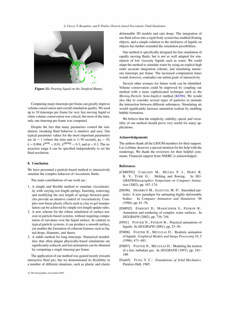
Figure 11: Pouring liquid on the Stanford Bunny.

Computing many timesteps per frame can greatly improvevolume conservation and overall simulation quality. We usedup to 10 timesteps per frame for very fast moving liquid orwhen volume conservation was critical, but most of the time,only one timestep per frame was computed.

Despite the fact that many parameters control the sim-ulation, tweaking fluid behavior is intuitive and easy. Ourtypical parameter values for the most important parametersare ∆t = 1 (where the time unit is 1/30 second), ρ0 = 10,k = 0.004, knear = 0.01, kspring = 0.3, and α = 0.3. The in-teraction range h can be specified independently to set thefluid resolution.

8. Conclusion

We have presented a particle-based method to interactivelysimulate the complex behavior of viscoelastic fluids.

The main contributions of our work are :

1. A simple and flexible method to simulate viscoelastic-ity with varying rest length springs. Inserting, removing,and modifying the rest length of springs between parti-cles provide an intuitive control of viscoelasticity. Com-plex non-linear plastic effects such as clay or gel manipu-lation can be achieved by simple rest length update rules.

2. A new scheme for the robust simulation of surface ten-sion in particle-based systems, without requiring compu-tation of curvature over the liquid surface. In contrast totypical particle systems, it can produce a smooth surface,yet enables the formation of coherent features such as liq-uid drops, filaments, and sheets.

3. A stable method for long timesteps. Numerical instabil-ities that often plague physically-based simulations aresignificantly reduced, and fast animations can be obtainedby computing a single timestep per frame.

The application of our method was geared mostly towardsinteractive fluid jets, but we demonstrated its flexibility ina number of different situations, such as plastic and elastic

deformable 3D models and rain drops. The integration ofour fluid solver into a rigid-body system has enabled floatingobjects, and a simple solution to the stickiness of liquids onobjects has further extended the simulation possibilities.

Our method is specifically designed for fast simulation ofrapidly moving fluids, but is not as well adapted for sim-ulation of low viscosity liquids such as water. We couldadapt the method to simulate water by using an explicit highorder accurate integration scheme, and simulating numer-ous timesteps per frame. The increased computation timeswould, however, contradict our initial goals of interactivity.

Several other avenues for future work can be identified.Volume conservation could be improved by coupling ourmethod with a more sophisticated technique such as theMoving-Particle Semi-Implicit method [KO96]. We wouldalso like to consider several types of particles to animatethe interaction between different substances. Simulating airwould significantly increase animation realism by enablingbubble formation.

We believe that the simplicity, stability, speed, and versa-tility of our method should prove very useful for many ap-plications.

Acknowledgements

The authors thank all the LIGUM members for their support.Luc Leblanc deserves a special mention for his help with therenderings. We thank the reviewers for their helpful com-ments. Financial support from NSERC is acknowledged.

References

[CMHT02] CARLSON M., MUCHA P. J., HORN R.B. V., TURK G.: Melting and flowing. In SIG-GRAPH/Eurographics Symposium on Computer Anima-tion (2002), pp. 167–174.

[DG96] DESBRUN M., GASCUEL M.-P.: Smoothed par-ticles: A new paradigm for animating highly deformablebodies. In Computer Animation and Simulation ’96(1996), pp. 61–76.

[EMF02] ENRIGHT D., MARSCHNER S., FEDKIW R.:Animation and rendering of complex water surfaces. InSIGGRAPH (2002), pp. 736–744.

[FF01] FOSTER N., FEDKIW R.: Practical animations ofliquids. In SIGGRAPH (2001), pp. 23–30.

[FM96] FOSTER N., METAXAS D.: Realistic animationof liquids. Graphical Models and Image Processing 58, 5(1996), 471–483.

[FM97] FOSTER N., METAXAS D.: Modeling the motionof a hot, turbulent gas. In SIGGRAPH (1997), pp. 181–188.

[Fun65] FUNG Y. C.: Foundations of Solid Mechanics.Prentice-Hall, 1965.



[GBF03] GUENDELMAN E., BRIDSON R., FEDKIW R.:Nonconvex rigid bodies with stacking. In SIGGRAPH(2003), pp. 871–878.

[GBO04] GOKTEKIN T. G., BARGTEIL A. W., O’BRIEN

J. F.: A method for animating viscoelastic fluids. In SIG-GRAPH (2004), pp. 463–468.

[GM77] GINGOLD R., MONAGHAN J.: Smoothed par-ticle hydrodynamics – theory and application to non-spherical stars. Monthly Notices of the Royal Astronomi-cal Society 181 (1977), 375.

[KO96] KOSHIZUKA S., OKA Y.: Moving-particle semi-implicit method for fragmentation of incompressiblefluid. Nuclear Science Engineering 123 (July 1996), 421–434.

[LC87] LORENSEN W. E., CLINE H. E.: Marching cubes:A high resolution 3D surface construction algorithm. InSIGGRAPH (1987), pp. 163–169.

[Luc77] LUCY L.: A numerical approach to the testing ofthe fission hypothesis. Astronomical Journal 82 (1977),1013.

[MCG03] MÜLLER M., CHARYPAR D., GROSS M.:Particle-based fluid simulation for interactive applica-tions. In SIGGRAPH/Eurographics Symposium on Com-puter Animation (2003), pp. 154–159.

[MKN∗04] MÜLLER M., KEISER R., NEALEN A.,PAULY M., GROSS M., ALEXA M.: Point based ani-mation of elastic, plastic and melting objects. In SIG-GRAPH/Eurographics Symposium on Computer Anima-tion (2004), pp. 141–151.

[Mor00] MORRIS J. P.: Simulating surface tension withsmoothed particle hydrodynamics. International Journalfor Numerical Methods in Fluids 33, 3 (2000), 333–353.

[MP89] MILLER G., PEARCE A.: Globular dynamics: Aconnected particle system for animating viscous fluids.Computers & Graphics 13, 3 (1989), 305–309.

[PIX] sourceforge.net/projects/pixie

[PTB∗03] PREMOŽE S., TASDIZEN T., BIGLER J.,LEFOHN A., WHITAKER R. T.: Particle-based simula-tion of fluids. Computer Graphics Forum 22, 3 (2003),401–410.

[Ree83] REEVES W. T.: Particle systems – a technique formodelling a class of fuzzy objects. In SIGGRAPH (1983),pp. 359–376.

[SCED04] STEELE K., CLINE D., EGBERT P. K., DIN-ERSTEIN J.: Modeling and rendering viscous liquids.Journal of Computer Animation and Virtual Worlds 15,3-4 (2004), 183–192.

[Sta99] STAM J.: Stable fluids. In SIGGRAPH (1999),pp. 121–128.

[THM∗03] TESCHNER M., HEIDELBERGER B.,

MUELLER M., POMERANETS D., GROSS M.: Op-timized spatial hashing for collision detection of de-formable objects. In Vision, Modeling, and Visualization(2003), pp. 47–54.

[TPF89] TERZOPOULOS D., PLATT J., FLEISCHER K.:Heating and melting deformable models (from goop toglop). In Graphics Interface (1989), pp. 219–226.

[VID] www.iro.umontreal.ca/labs/infographie/papers

Appendix – Prediction-Relaxation Scheme

The integration scheme we use can be written as

x∗ = xn +∆t vn− 12

x∗ ← x∗ +∆t2 F1(x∗)/m

x∗ ← x∗ +∆t2 F2(x∗)/m

x∗ ← x∗ +∆t2 F3(x∗)/m

...

xn+1 = x∗vn+ 1

2= (xn+1−xn)/∆t.

This sequential application of force components is analo-gous to operator splitting often used in Eulerian simula-tions [Sta99]. Each stage of force application uses the pre-viously updated position, which can lead to greater stability.For example, it is intuitively correct to compute collisionsusing positions that have already been modified by otherconstraints. Allowing a particular constraint to adjust to whathappened in previous stages often prevents overshoots anderroneous constraint responses.

If only one force is used, the integration scheme can besimplified to

vn+ 12

= vn− 12+∆t F(xn +∆t vn− 1

2)/m

xn+1 = xn +∆t vn+ 12

which is similar to the usual leap-frog scheme, but with theforce computed at the predicted position. Testing the canon-ical example F =−k x leads to

vn+ 12

= vn− 12+∆t (−k xn− k ∆t vn− 1

2)/m

in which the actual force being computed is augmented withthe term −k ∆t vn− 1

2, an artificial viscosity.



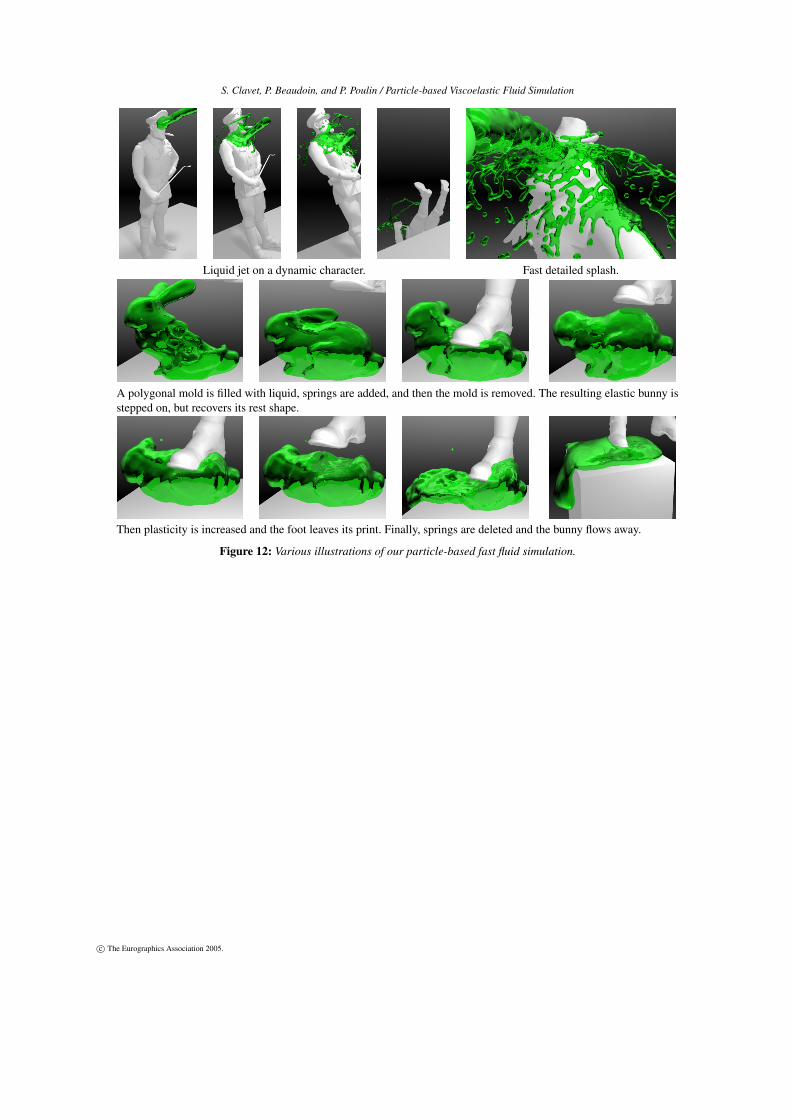
Liquid jet on a dynamic character. Fast detailed splash.

A polygonal mold is filled with liquid, springs are added, and then the mold is removed. The resulting elastic bunny isstepped on, but recovers its rest shape.

Then plasticity is increased and the foot leaves its print. Finally, springs are deleted and the bunny flows away.

Figure 12: Various illustrations of our particle-based fast fluid simulation.


Documents

Particle-based Viscoelastic Fluid Simulation · S. Clavet, P. Beaudoin, and P. Poulin / Particle-based Viscoelastic Fluid Simulation allows for direct specication of well-dened physical