Embed Size (px)
Citation preview
Particle dissolution and cross-diffusion in multi-component alloys
F.J. Vermolen a,*, C. Vuik a, S. van der Zwaag b,c
a Department of Applied Mathematical Analysis, Delft University of Technology, Mekelweg 4, 2628 CD Delft, The Netherlandsb Laboratory of Materials Science, Delft University of Technology, Rotterdamse weg 137, 2628 AL Delft, The Netherlands
c Netherlands Institute for Metals Research (N.I.M.R.), Rotterdamse weg 137, 2628 AL Delft, The Netherlands
Received 26 April 2002; received in revised form 31 July 2002
Abstract
A general model for the dissolution of stoichiometric particles, taking into account the influences of cross-diffusion, in multi-
component alloys is proposed and analyzed using a diagonalization argument. It is shown that particle dissolution in multi-
component alloys with cross-diffusion can under certain circumstances be approximated by a model for particle dissolution in
binary alloys. Subsequently, the influence of cross-diffusion on particle dissolution rate is analyzed for planar and spherical
particles. Further, we show some numerical simulations and conclude that cross-diffusion can be incorporated into multi-
component dissolution models.
# 2002 Elsevier Science B.V. All rights reserved.
Keywords: Multi-component alloy; Particle dissolution; Cross-diffusion; Vector-valued Stefan problem; Self-similar solution
1. Introduction
In the thermal processing of both ferrous and non-
ferrous alloys, homogenization of the as-cast micro-
structure by annealing at such a high temperature that
unwanted precipitates are fully dissolved, is required to
obtain a microstructure suited to undergo heavy plastic
deformation. Such a homogenization treatment, to
name just a few examples, is applied in hot-rolling of
Al killed construction steels, HSLA steels, all engineer-
ing steels, as well as aluminium extrusion alloys.
Although precipitate dissolution is not the only metal-
lurgical process taking place, it is often the most critical
of the occurring processes. The minimum temperature at
which the annealing should take place can be deter-
mined from thermodynamic analysis of the phases
present. Another important quantity is the minimum
annealing time at this temperature. This time, however,
is not a constant but depends on particle size, particle
geometry, particle concentration, overall composition
etc.
Due to the scientific and industrial relevance of being
able to predict the kinetics of particle dissolution, many
models of various complexity have been presented and
experimentally validated. The early models on particle
dissolution based on long-distance diffusion were based
on analytical solutions in an unbounded medium under
the assumption of local equilibrium at the moving
interface, see Whelan [1] for instance. The model of
Nolfi et al. [2] incorporate the interfacial reaction
between the dissolving particle and its surrounding
phase. Later modeling particle dissolution has been
extended to the introduction of multi-component parti-
cles by, among others, Reiso et al. [3], Hubert [4]. All the
above mentioned models were based on viewing particle
dissolution as a Stefan problem. A recent approach is
the phase-field approach, which is derived from a
minimization of the energy functional. This approach
has, among others, been used by Kobayashi [5] to
simulate dendritic growth. A recent extension to multi-
component phase-field computation is done by Grafe et
al. [6], where solidification and solid state transforma-
tions are modeled. For the one-dimensional case they
obtain a perfect agreement between the phase-field
approach and the software package DICTRA which is
based on a sharp interface between constituent phases.
Some disadvantages of the phase-field approach are that
* Corresponding author. Tel.: �/31-15-278-1833; fax: �/31-15-278-
7209.
E-mail address: [email protected] (F.J. Vermolen).
Materials Science and Engineering A347 (2003) 265�/279
www.elsevier.com/locate/msea
0921-5093/02/$ - see front matter # 2002 Elsevier Science B.V. All rights reserved.
PII: S 0 9 2 1 - 5 0 9 3 ( 0 2 ) 0 0 6 1 5 - 9
(1) no simple quick estimates of the solution are
available and (2) physically justifiable parameter values
in the energy functional are not easy to obtain: generally
these quantities are to be obtained by using fittingprocedures that link experiment and numerical compu-
tation. Therefore, we limit ourselves in the present work
to model particle dissolution as a Stefan problem, where
a multi-component ‘generalized’ Fick diffusion equation
including cross-diffusion coefficients has to be solved
with a moving interface separating the constituent solute
and solvent phases.
Kale et al. [7] consider ternary diffusion in FCCphases of Fe�/Ni�/Cr alloy systems. They compute
diffusion coefficients, including cross-diffusion coeffi-
cients, by using the thermodynamically based
Boltzmann�/Matano method. In their metallic systems
the cross-diffusion coefficients range in value up to
about a third of those of the diagonal diffusion
coefficients. Hence cross-diffusion should be taken
into account here. Vergara et al. [8] recently emphasizedthe significance of cross-terms in the ‘generalized’ Fick
diffusion equation. They construct a model to evaluate
(cross) diffusion coefficients from experiments. They
apply their model to a reference system containing
Sodiumchloride in water, Travis and Gubbins [9]
compute cross-diffusion coefficients in graphite slit
pores using Monte-Carlo simulations. The formalism
of cross-diffusion in multi-component metallic alloyshas been motivated in terms of chemical potentials by
Kirkaldy and Young [10]. In their work, an analytical
solution of the obtained system of diffusion equations
has been given for a one-dimensional and unbounded
geometry. They note that the eigenvalues of the diffu-
sion matrix have to be real-valued and positive for an
acceptable physical problem. A more recent book where
cross-diffusion is also treated is the book of Glicksman[11]. Here a self-similar solution of the equations is given
where the boundaries are fixed. A numerical solution of
the diffusion equations for fixed boundaries including
cross-diffusion was recently obtained by Naumann and
Savoca [12].
As far as we know, no extension to problems that
incorporate the movement of the interface has been
made yet. It is the aim of this work to analyze thecombination of a moving boundary with cross-diffusion
effects. Existence of (multiple) solutions when the
diffusion matrix is singular is stated and proven as
mathematical theorems in [13]. In the present study, we
give asymptotic solutions for the dissolution of a planar
and spherical particle. Furthermore, we show that under
certain circumstances the multi-component problem
with cross-diffusion terms (a strongly coupled ‘vector-valued’ Stefan problem) can be approximated by a
binary problem (‘scalar’ Stefan problem). Subsequently
we present a numerical method that is used to solve the
Stefan problem and give some numerical results for
hypothetical alloys. Finally some conclusions are pre-
sented.
We remark that this study is an extension of earlier
work described in [14�/16] where influences of cross-diffusion on the dissolution problem were not incorpo-
rated yet.
2. Basic assumptions in the model
The as-cast microstructure is simplified into a repre-sentative cell containing the ‘matrix’ of phase a and a
single particle of phase b of a specific form, size and
location of the cell boundary. To avoid confusion we use
the notation ‘matrix’ for a phase surrounding the
dissolving particle and the notation matrix to indicate
the mathematical notion of a two-dimensional array of
numbers.
Both a uniform and a spatially varying initialcomposition at t�/0 can be assumed in the model. The
boundary between the b-particle and a-‘matrix’ is
referred to as the interface. Particle dissolution is
assumed to proceed by a number of the subsequent
steps [2]: decomposition of the particle, atoms from the
particle crossing the interface and diffusion of these
atoms in(to) the a-phase. Here we take the effects of
cross-diffusion into account. We assume in this workthat the first two mechanisms proceed sufficiently fast
with respect to diffusion. Hence, the interfacial concen-
trations are those as predicted by thermodynamics (local
equilibrium).
In [15], we considered the dissolution of a stoichio-
metric particle in a ternary and a general multi-
component alloy. We denote the chemical species by
Spi , i � /{l, . . ., n�/1}, where Spn�1 is the ‘original’solvent metallic a-phase in which the particle dissolves.
We denote the stoichiometry of the particle by
(Sp1)m1(Sp2)m
2(Sp3)m
3(. . .)(Spn)m
n. The numbers m1, m2,
. . ., mn are stoichiometric constants. We denote the
interfacial concentration of species i by cisol and we use
the following hyperbolic relationship for the interfacial
concentrations:
(csol1 )m1 (csol
2 )m2 (. . .)(csoln )mn �K : (1)
The factor K is referred to as the solubility product. Itdepends on temperature T according to an Arrhenius
relationship, in the present work, however, we assume it
to be constant.
We denote the position of the moving interface
between the b-particle and a-phase by S (t), where t
denotes time. Consider a one-dimensional domain, i.e.
there is one spatial variable, which extends from 0 up to
M (the cell size). Since particles dissolve simultaneouslyin the metal, the concentration profiles between con-
secutive particles may interact and hence soft-impinge-
ment occurs. This motivates the introduction of a
F.J. Vermolen et al. / Materials Science and Engineering A347 (2003) 265�/279266

finitely sized cell over whose boundary there is no flux.
For cases of low overall concentrations in the alloy, the
cell size M may be large and the solution resembles the
case where M is infinite. The spatial co-ordinate isdenoted by r , 05/S (t )5/r 5/M . This domain is referred
to as V (t )�/{r � /R: S(t)5/r 5/M}. The a-‘matrix’,
where diffusion takes place, is given by V (t ) and the
b-particle is represented by the domain 05/r 5/S (t).
Keeping cross-diffusion in mind, we have for each
alloying element, with r � /V (t) and t �/0:
@ci
@t�
Xn
j�1
1
ra
@
@r
�Dijr
a @cj
@r
�; for i � f1; . . . ; ng: (2)
The geometry is planar, cylindrical and spherical for,
respectively, a�/0, 1 and 2. The above equations follow
from thermodynamic considerations, their derivation
can for instance be found in [10]. Here Dij and ci ,
respectively, denote the coefficients of the diffusion
matrix and the concentration of the species i in the a-rich phase. The diffusion matrix D is notated as follows:
D�D11 . . . D1n
. . . . . . . . .
Dn1 . . . Dnm
0@
1A: (3)
The off-diagonal entries of D (i.e. Dij , i "/j), also
referred to as the cross-terms, are a measure for the
interaction of diffusion in the ’matrix; between con-
secutive alloying elements. When an alloying element is
dissolved in the a-‘matrix’ then the resulting stress andelongations in the crystal structure facilitate or worsen
diffusion of the other elements. The off-diagonal entries
of D are a measure of for this mutual influence. When
Dij B/0, then alloying element j deteriorates diffusion of
element i in the a-‘matrix’, whereas Dij �/0 implies that
element j facilitates diffusion of element i in the a-
‘matrix’. An alternative formulation of cross-diffusion is
treated by Farkas [17] where only the diagonal entries ofthe above diffusion matrix are used, however, these
diagonals are taken to depend on the concentration of
all the other species and hence a strong coupling arises
in a different way. We do not treat this approach in this
study but we will use the formulation of Eq. (2) that has
been motivated in [10]. We further assume that the
diffusion matrix does not depend on the concentration,
time and space, i.e. the matrix is treated as a constant inthe present work. We note that the matrix D generally
depends on time when the particle dissolves during a
non-isothermal heat treatment.
Let ci0 denote the initial concentration of each element
in the a-phase, then we take as initial conditions (IC):
(IC)ci(r; 0)�c0
i (r) for i � f1; . . . ; ngS(0)�S0:
�(4)
At a boundary not being an interface, i.e. at M or
when S (t )�/0; we assume no flux through it, i.e.:
Xn
j�1
Dij
@cj
@n�0; for i � f1; . . . ; ng: (5)
Here n represents the outward normal vector of a cell.
When D is not singular, then Eq. (5) holds if and only if:
@ci
@n�0; for i � f1; . . . ; ng: (6)
Furthermore at the moving interface S (t ) we have the‘Dirichlet boundary condition’ ci
sol for each alloying
element. The concentration of element i in the particle is
denoted by cipart, this concentration is fixed at all stages.
This assumption follows from the constraint that the
stoichiometry of the particle is maintained during
dissolution in line with Reiso et al. [3]. The dissolution
rate (interfacial velocity) is obtained from a mass-
balance of the atoms of alloying element i . The mass-balance per unit area leads to:
(S(t � Dt) � S(t))
Dt(cpart
i �csoli )�
Xn
j�1
Dij
@cj
@r(S(t); t): (7)
Subsequently we take the limit Dt 0/0 and we obtain
the following equation for the interfacial velocity:
(cparti �csol
i )dS
dt�
Xn
j�1
Dij
@cj
@r: (8)
Summarized, we obtain at the interface for t �/0 and
i , j � /{1, . . ., n}:
ci(S(t); t)�csoli
(cparti �csol
i )dS
dt�
Xn
j�1
Dij
@cj
@r(S(t); t)
g[
Xn
k�1
Dik
cparti � csol
i
@ck
@r(S(t); t)
�Xn
k�1
Djk
cpartj � csol
j
@ck
@r(S(t); t) (9)
The right-hand side of above equations follows fromlocal mass-conservation of the components. Above
formulated problem falls within the class of Stefan-
problems, i.e. diffusion with a moving boundary. Since
we consider simultaneous diffusion of several chemical
elements, it is referred to as a ‘vector-valued Stefan
problem’. The unknowns in above equations are the
concentrations ci , interfacial concentrations cisol and the
interfacial position S (t), All concentrations are bynecessity non-negative. The coupling exists in both the
diffusion equations, Stefan condition and the values of
the concentrations at the interfaces between the particle
F.J. Vermolen et al. / Materials Science and Engineering A347 (2003) 265�/279 267

and a-rich phase. This strong coupling complicates the
qualitative analysis of the equations. For a mathema-
tical overview of Stefan problems we refer to the
textbooks of Crank [18], Chadarn and Rasnmssen [19]and Visintin [20].
3. Analysis
In this section, we factorize the diffusion matrix by
use of its eigenvalues and (generalized) eigenvectors
according to standard linear algebra procedures. This is
done to facilitate the mathematical problem that has to
he solved. A direct consequence of the factorization is
that the cross-terms in the equations vanish and the
diffusion coefficients are replaced by the eigenvalues of
the diffusion matrix. In most cases the diffusion matrixis diagonalizable and the strong coupling vanishes
between the diffusion equations. However, when the
diffusion matrix is not diagonalizable then some or one
diffusion equation is uncoupled whereas the rest of the
diffusion equations are coupled. Further, the solution of
the transformed diffusion equations in general no longer
satisfies a maximum principle and hence extremes away
from the boundaries may be present also for t �/0 whenthe diffusion matrix is not diagonalizable. We refer to
[13] for a more extensive treatment. The analytical
solutions that we present here are based on self-
similarity and for an unbounded domain.
3.1. Decomposition of the diffusion matrix
First we write the equations in a vector-notation and
we define the vectors c¯�/(c1, c2, . . ., cn)T, c
¯
p�/(c1part,
c2part, . . ., cn
part)T and c¯
s�/(c1sol, c2
sol, . . ., cnsol)T, then the
diffusion equations can be written as:
@
@t ¯c�
1
ra
@
@r
�raD
@
@r
�¯c: (10)
The boundary and IC follow similarly in vector
notation. The Stefan condition becomes in vector
notation:
(¯cp�
¯cs)
dS
dt�
@
@rD
¯c(S(t); t): (11)
We assume that the matrix D is diagonalizable. To
analyze Eq. (11) we use the Decomposition Theorem,
which can for instance be found in [21], page 317. Thetheorem says that for each real-valued n �/n-matrix D
there exists a non-singular n �/n -matrix P such that:
D�PLP�1; (12)
where L is a diagonal matrix containing the eigenvalues
of matrix D :
L�
l1 0 0 . . . 0
0 l2 0 0 . . . 0
0 0 l3 0 . . .
0 . . . . . . . . . . . . ln
0BB@
1CCA: (13)
In our case the set {ln} correspond to the eigenvalues of
the diffusion matrix D .
The matrix P has columns that are formed by the
eigenvectors of D . The arrangement is in the same order
as the set {ln} in the matrix L , The eigenvalues and
eigenvectors are obtained from:
det(D�lI)�0; giving fl1; . . . ; lng (14)
D¯vi�li
¯vi; (15)
note that some of the eigenvalues may be equal.
When the matrix D is not diagonalizable, we consider
an eigenvalue li of multiplicity p in Eq. (14). For this
case, we have lj �/li for j � /{i , . . ., i�/p}. The general-
ized eigenvectors that are substituted into the columns
of P are obtained from:
D¯vi�li
¯vi; (16)
(D�liI)¯vj�1�
¯vj; for j � fi; . . . ; i�p�1g: (17)
In the second equation above we assume that lj �/li
for all j � /{i , . . ., i�/p} and that v¯j depends linearly on its
preceding eigenvectors. In Eq. (17), I is the n �/n-
identity matrix. Further, L becomes a Jordan blockmatrix when D is not diagonalizable. We refer to [13] for
a more extensive treatment of the case where D is not
diagonalizable.
We remark that Kirkaldy et al. [22] use a thermo-
dynamic argument to show that the eigenvalues of the
diffusion matrix are positive and real-valued. Therefore,
we limit ourselves to cases where the eigenvalues are
real-valued and positive.
3.1.1. An example for a ternary alloy
We consider a ternary example, with the following
real-valued matrix:
D�D11 D12
D21 D22
�� (18)
From Eq. (14) follows that the eigenvalues are
determined from:
(D11�l)(D22�l)�D12D21�0U (19)
Ul�
D11 � D22 9
ffiffiffiffiffiffiffiffiffiffiffiffiffiffiffiffiffiffiffiffiffiffiffiffiffiffiffiffiffiffiffiffiffiffiffiffiffiffiffiffiffiffiffiffiffiffiffiffiffiffiffiffiffiffiffiffiffiffiffiffiffiffiffiffiffiffiffiffiffiffiffiffiffiffi(D11 � D22)2 � 4(D11D22 � D12D21)
q2
(20)
We remark that when the trace of D is positive,
tr(D )�/D11�/D22�/0, and:
F.J. Vermolen et al. / Materials Science and Engineering A347 (2003) 265�/279268

det(D)�D11D22�D12D21 �
0;
tr(D)2
4
�; (21)
then the eigenvalues of D are real and have a positivevalue.
3.2. Transformation of the diffusion equations
For the remaining text we assume that the eigenvalues
of D are real and positive. Substitution of the decom-
position of D , Eq. (12) into Eq. (11) gives:
@
@t ¯c�
1
ra
@
@r
�ra @
@r
�PLP�1
¯cU
@
@tP�1
¯c
�1
ra
@
@r
�ra @
@r
�LP�1
¯c
(¯cp�
¯cs)
dS
dt�
@
@rPLP�1
¯c(S(t); t)UP�1(
¯cp�
¯cs)
dS
dt
�@
@rLP�1
¯c(S(t); t): (22)
We define the transformed concentrations as:
¯u�P�1
¯c;
¯us�P�1
¯cs; up�P�1
¯cp;
¯u0�P�1
¯c0:
(23)
Then the diffusion equation and equation of motion
change into:
@
@t ¯u�
1
ra
@
@r
�ra @
@r
�L
¯u (24)
(¯up�
¯us)
dS
dt�
@
@rL
¯u(S(t); t): (25)
Note that the system given in Eq. (24) is fully
uncoupled. The homogeneous Neumann conditions atthe non-moving boundary are similar for the trans-
formed concentrations. Further, we have for t�/0.
uj �u0
j ; for r � (S(0); M];
upartj ; for r � [0; S(0)]:
j � f1; . . . ; ng�
(26)
From¯c�P
¯u[ci�a
n
j�1 pijuj; the coupling between
the interfacial concentrations via the hyperbolic relation
Eq. (1) changes into:Xn
j�1
p1jusj
�m1Xn
j�1
p2jusj
�m2
(. . .)
Xn
j�1
pnjusj
�mn
�K : (27)
The analysis is facilitated using the diagonalization ofthe diffusion matrix. We see that the coupling between
subsequent concentrations only remains in the above
Eqs. (27) and (25).
4. Similarity solutions and asymptotic approximations
We consider analytical solutions satisfying Eq. (2) for
the concentrations. We illustrate the importance ofcross-diffusion in the above problem by the use of the
exact self-similar solution for problem (P1), which is
derived in [13] for the planar case, where a�/0 in Eq.
(24), Fig. 1 displays dissolution curves computed for
various values of cross-diffusion coefficient D12 where
we use the following data-set:
¯c0�(0; 0)T
¯cpart�(50; 50)T; D�
1 D12
D12 2
�;
K�1:(28)
The above diffusion matrix is symmetric. From Fig. 1,
it is clear that the influence of the cross-terms issignificant. Since Kale et al. [7] indicate that the cross-
diffusion terms can have the same order of magnitude as
the diagonal terms in the diffusion matrix we choose the
values of D12 in the range [�/1, 0].
We, however, will use the approximation by Aaron
and Kotler [23] for the planar case and the approxima-
tion by Whelan [1] for the spherical case. Both
approaches are derived with the use of Laplace trans-forms where the interfacial position is assumed to move
far more slowly than the rate of diffusion in the a-
‘matrix’. This turns out to be a good approximation
when juis�/ui
0j�/juip�/ui
sj. This is illustrated in some
examples in the remainder of this section. With both
approches an easy solvable problem arises for the
estimation of the dissolution rate for a planar and
spherical particle in a multi-component alloy with cross-diffusion. We will only discuss this for the case of a
diagonalizable diffusion matrix. The case of a non-
diagonalizable matrix is more complicated but can be
treated analogously, see [13] for more details on the
mathematics for the non-diagonalizable case. For the
planar case, we give an estimate for the dissolution rate
in terms of a quasi-binary formulation of the multi-
component dissolution problem with cross-diffusion.Finally, we use the Whelan [1] approach to obtain a
semi-analytical approach for the spherical case.
4.1. An asymptotic solution for the planar case
Suppose that juis�/ui
0j�/juip�/ui
sj then Aaron andKotler [23] give the following equation for interface
motion for a given combination of uis, ui
p and ui0:
dS
dt�
u0i � us
i
upi � us
i
ffiffiffiffiffili
pt
s“
k
2ffiffit
p : (29)
Since the solution for dS /dt should be the same for all
components i , this implies with combination with Eq.
(27) that the solution of problem (P1) is approximated
F.J. Vermolen et al. / Materials Science and Engineering A347 (2003) 265�/279 269

by the solution for k and uis of:
(P1)
k�2u0
i � usi
upi � us
i
ffiffiffiffiffiffili
p;
sfor i � f1; . . . ; ng;
Xn
j�1
p1jusj
�m1Xn
j�1
p2jusj
�m2
(. . .)
Xn
j�1
pnjusj
�mn
�K
8>>>><>>>>:
The above problem follows from the approach due to
Aaron and Kotler [23] and can be solved by using a,
zero-point method. The derivation of this approach is
based on the Laplace transform of the diffusion
equation. The approach can also be derived from theexact self-similar solution, this is done in [13]. We
continue on a simplification of the above problem to
obtain an explicit solution. Suppose that the initial
concentrations are zero, then¯u0�
¯0 and hence that the
transformed particle concentration is much larger than
the transformed interfacial concentrations, i.e. uis�/ui
p
for i � /{1, . . ., n} then the first equation of (P1) with i�/1
becomes:
k:�2us
1
up1
ffiffiffiffiffil1
p
s: (30)
Hence the equation of motion of the interface
becomes
dS
dt:�
us1
up1
ffiffiffiffiffil1
pt
s: (31)
Further, the following recurrence relation between the
transformed interfacial concentrations follows:
Substitution of above transformed interfacial concen-
trations into the second equation of (P2) gives the
following real-valued solution:
where we defined m�anj�1mj: Above expression for the
transformed interfacial concentration is substituted into
Fig. 1. The interface position as a function of time for the exact self similar solution for several values of the cross-diffusion terms.
us1�
KXn
j�1
p1j
upj
up1
ffiffiffiffiffil1
lj
s �m1Xn
j�1
p2j
upj
up1
ffiffiffiffiffil1
lj
s �m2
(. . .)
Xn
j�1
pnj
upj
up1
ffiffiffiffiffil1
lj
s �mn
�1=m
; (33)
usi �
upi
up1
ffiffiffiffiffil1
li
sus
1: (32)
F.J. Vermolen et al. / Materials Science and Engineering A347 (2003) 265�/279270
the rate equation for the interface (Eq. (30)). This gives:
dS
dt��
K1=m
up1
�Yn
k�1
1
(Xn
j�1
(pkj(upj =u
p1
ffiffiffiffiffiffiffiffiffiffiffil1=lj
q)))mk
�1=m
�ffiffiffiffiffil1
pt
s: (34)
The above equation is referred to as the quasi-binaryapproach or as the effective approximation. From the
above equation dissolution times of the particle can be
estimated easily using known parameters such as the
eigenvalues and eigenvectors of the diffusion matrix.
Furthermore, the solubilities obtained from the above
equations can be used as initial guesses for the zero-
point method to solve for the semi-explicit solution and
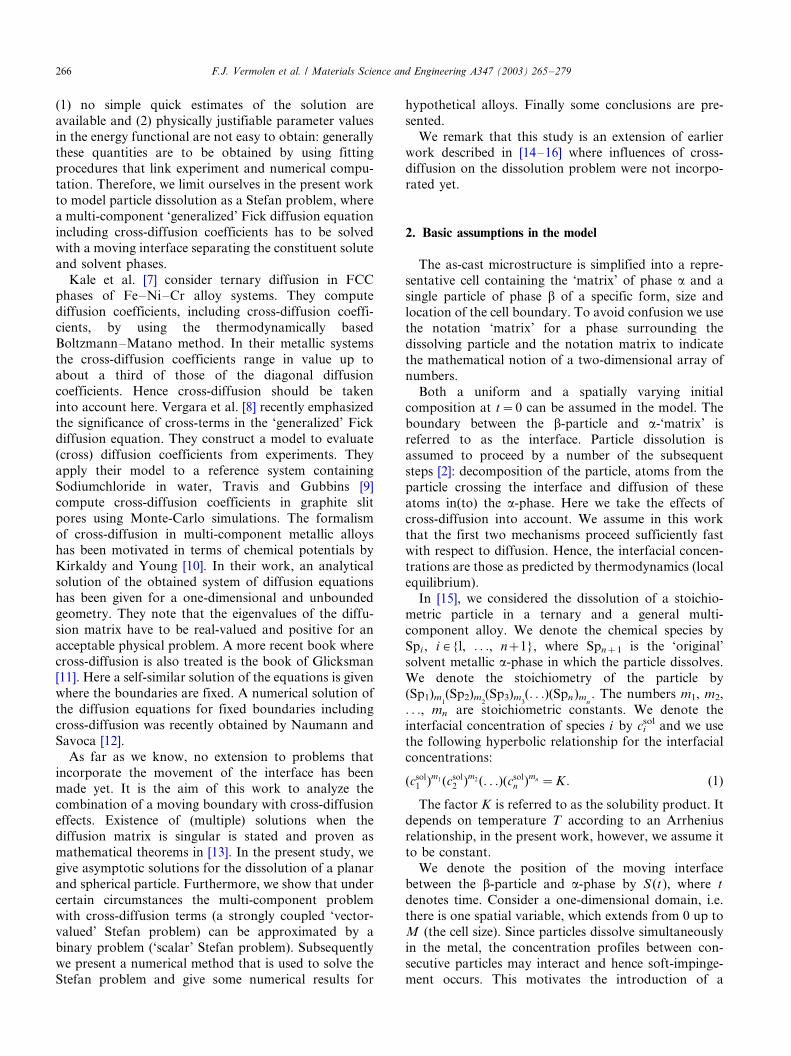
numerical solutions.In Fig. 2 we show the interface position, computed by
the use of the exact ‘Neumann’ solution for the planar
case (see [13]), (P1) (the’Aaron’ approximation) and Eq.
(34) (the ‘effective’ approximation), as a function of time
for K�/1 and c¯
p�/(50, 50)T, c¯
p�/(15, 15)T and c¯
p�/(5,
5)T. The other data are the same as in Fig. 1. It can be
seen that for high particle concentrations c¯
p�/(50, 50)T
the difference between all the approaches is small.Whereas for lower particle concentrations the difference
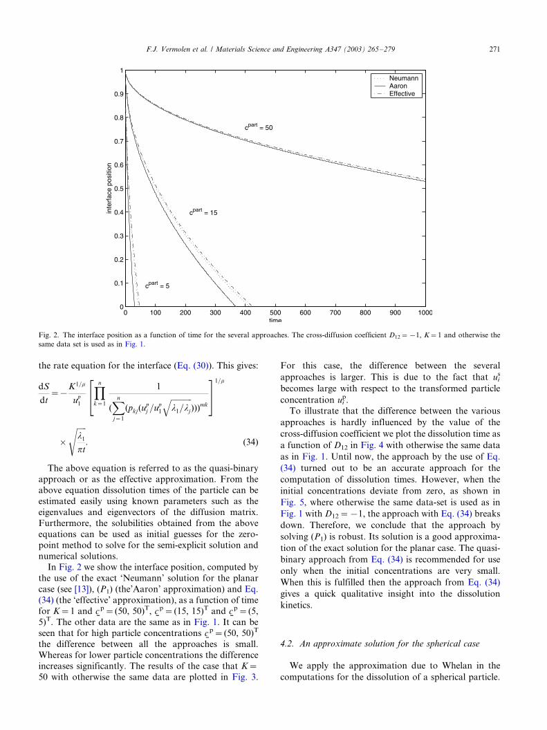
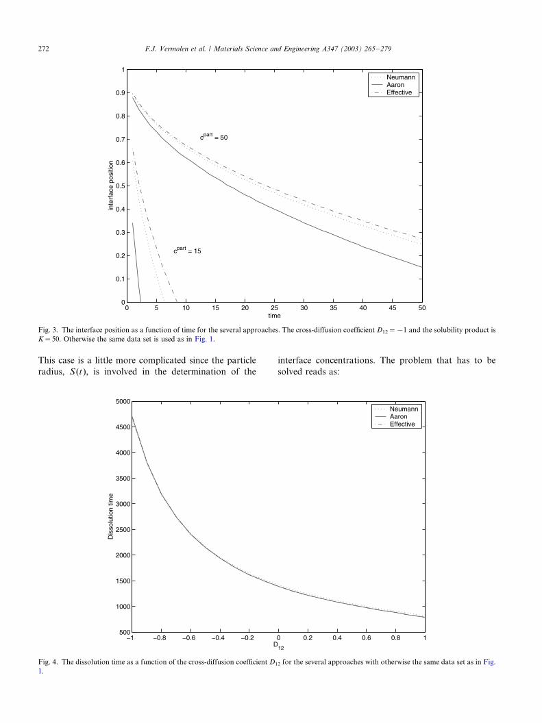
increases significantly. The results of the case that K�/
50 with otherwise the same data are plotted in Fig. 3.
For this case, the difference between the several
approaches is larger. This is due to the fact that uis
becomes large with respect to the transformed particle
concentration uip.
To illustrate that the difference between the various
approaches is hardly influenced by the value of the
cross-diffusion coefficient we plot the dissolution time as
a function of D12 in Fig. 4 with otherwise the same data
as in Fig. 1. Until now, the approach by the use of Eq.
(34) turned out to be an accurate approach for the
computation of dissolution times. However, when the
initial concentrations deviate from zero, as shown in
Fig. 5, where otherwise the same data-set is used as in
Fig. 1 with D12�/�/1, the approach with Eq. (34) breaks
down. Therefore, we conclude that the approach by
solving (P1) is robust. Its solution is a good approxima-
tion of the exact solution for the planar case. The quasi-
binary approach from Eq. (34) is recommended for use
only when the initial concentrations are very small.
When this is fulfilled then the approach from Eq. (34)
gives a quick qualitative insight into the dissolution
kinetics.
4.2. An approximate solution for the spherical case
We apply the approximation due to Whelan in the
computations for the dissolution of a spherical particle.
Fig. 2. The interface position as a function of time for the several approaches. The cross-diffusion coefficient D12�/�/1, K�/1 and otherwise the
same data set is used as in Fig. 1.
F.J. Vermolen et al. / Materials Science and Engineering A347 (2003) 265�/279 271
This case is a little more complicated since the particle
radius, S (t ), is involved in the determination of the
interface concentrations. The problem that has to be
solved reads as:
Fig. 3. The interface position as a function of time for the several approaches. The cross-diffusion coefficient D12�/�/1 and the solubility product is
K�/50. Otherwise the same data set is used as in Fig. 1.
Fig. 4. The dissolution time as a function of the cross-diffusion coefficient D12 for the several approaches with otherwise the same data set as in Fig.
1.
F.J. Vermolen et al. / Materials Science and Engineering A347 (2003) 265�/279272

Fig. 5. The dissolution time as a function of the initial concentration ci0�/c0 for D12�/�/1 with otherwise the same data as in Fig. 1.
Fig. 6. The interfacial position of a spherical particle as a function of time for the ‘Whelan’ solution for several values of the cross-diffusion terms.
Otherwise the same data set as in Fig. 1 is used.
F.J. Vermolen et al. / Materials Science and Engineering A347 (2003) 265�/279 273

Find S (t ) and u¯
s such that
dS
dt�
u0i � uS
i
upi � uS
i
ffiffiffiffiffili
pt
s�
li
S
�Xn
j�1
P1juSj
�m1Xn
j�1
P2juSj
�m2
(. . .)
Xn
j�1
PnjuSj
�mn
�K
8>>>><>>>>:
(35)
The above problem is solved with the use of combina-
tion of a zero-point method to obtain uSi combined with
a time-integration method to obtain S (t). We show
some results in Figs. 6 and 7 where we plot the sphereradius and interface concentrations as a function of
time. In constrast to the planar case, it can be seen that
the interfacial concentrations do not stay constant.
However, we observed that the interface concentrations
and interface velocity are equal to the values from the
planar case at the very early stages of dissolution (as t 0/
0). This agrees perfectly with the expectations. Further-
more, a similar effective approach as in Section 4.1 canbe derived for the spherical case for sufficiently large t .
5. Numerical experiments
We solved the treated problem for particle dissolution
in multi-component alloys with cross-diffusion numeri-
cally for a bounded domain. The method is based on
Finite Differences combined with a classical moving grid
method for the determination of the interface position.
Further, the interface concentrations are obtained by an
approximate Newton method. The details are described
in [15,13].
This section displays some numerical simulations for
hypothetical alloys. First we treat an example where thediffusion matrix is diagonalizable and subsequently a
non-diagonalizable case is considered.
5.1. The diagonalizable case
As a numerical experiment we show the computation
of the dissolution of a planar phase for the case that the
diffusion matrix is diagonalizable. Furthermore, we
compare the computed numerical solutions with the
self-similar solution as developed in Section 4. As input-
data we used
¯c0�(0; 0)T;
¯cpart�(50; 50)T;
D�1 �1=4
�1=4 2
�; K�1:
(36)
The above matrix is diagonalizable. In Fig. 8, we plot
the interface as a function of time for the (approximate)
self-similar solution and the numerical solution. Sincecpart
i �/csoli �/c0
i �/0 we can approximate the solution of
(P1) by the use of Eq. (34). Hence the analytical
approaches coincide. At early stages the concentration
Fig. 7. The interfacial concentrations as a function of time for the ‘Whelan’ solution for several values of the cross-diffusion terms. Otherwise the
same data set as in Fig. 1 is used.
F.J. Vermolen et al. / Materials Science and Engineering A347 (2003) 265�/279274

profiles resemble the profiles that are obtained from the
similarity solutions. As time proceeds the dissolution is
delayed by soft-impingement at the cell boundary. At
this stage, the curve that has been obtained from the
numerical computations starts to deviate from the
analytical approaches. This effect is clearly visible in
Fig. 8. The interfacial position as a function of time. The dotted curve corresponds to self-similar solution and the solid curve corresponds to the
numerical approach.
Fig. 9. The interface position as a function of time for the case that the diffusion matrix is not diagonalizable. The analytical and numerical solution
are shown.
F.J. Vermolen et al. / Materials Science and Engineering A347 (2003) 265�/279 275
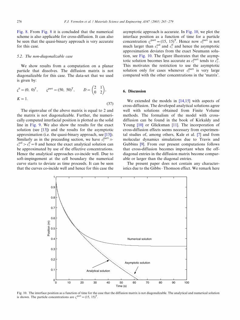
Fig. 8. From Fig. 8 it is concluded that the numerical
scheme is also applicable for cross-diffusion. It can also
be seen that the quasi-binary approach is very accurate
for this case.
5.2. The non-diagonalizable case
We show results from a computation on a planar
particle that dissolves. The diffusion matrix is not
diagonalizable for this case. The data-set that we used
is given by:
¯c0� (0; 0)T;
¯cpart�(50; 50)T; D�
2 1
0 2
�;
K�1:(37)
The eigenvalue of the above matrix is equal to 2 and
the matrix is not diagonalizable. Further, the numeri-
cally computed interfacial position is plotted as the solid
line in Fig. 9. We also show the results for the exact
solution (see [13]) and the results for the asymptotic
approximation (i.e. the quasi-binary approach, see [13]).
Similarly as in the preceeding section, we have cipart�/
cisol�/ci
0�/0 and hence the exact analytical solution can
be approximated by use of the effective concentrations.
Hence the analytical approaches co-incide well. Due to
soft-impingement at the cell boundary the numerical
curve starts to deviate as time proceeds. It can be seen
that the curves co-incide well and hence for this case the
asymptotic approach is accurate. In Fig. 10, we plot the
interface position as a function of time for a particle
concentration c¯
part�/(15, 15)T. Hence now cipart is not
much larger than cisol and ci
0 and hence the asymptoticapproximation deviates from the exact Neumann solu-
tion, see Fig. 10. The figure illustrates that the asymp-
totic solution becomes less accurate as cipart tends to ci
0.
This motivates the restriction to use the asymptotic
solution only for cases whenever cipart is very large
compared with the other concentrations in the ‘matrix’.
6. Discussion
We extended the models in [14,15] with aspects ofcross-diffusion. The developed analytical solutions agree
well with solutions obtained from Finite Volume
methods. The formalism of the model with cross-
diffusion can be found in the book of Kirkaldy and
Young [10] or Glicksman [11]. The incorporation of
cross-diffusion effects seems necessary from experimen-
tal studies of, among others, Kale et al. [7] and from
molecular dynamics simulations due to Travis andGubbins [9]. From our present computations follows
that cross-diffusion becomes important when the off-
diagonal entries in the diffusion matrix become compar-
able or larger than the diagonal entries.
The present paper does not contain any character-
istics due to the Gibbs�/Thomson effect. We remark here
Fig. 10. The interface position as a function of time for the case that the diffusion matrix is not diagonalizable. The analytical and numerical solution
is shown. The particle concentrations are c¯
part�/(15, 15)T.
F.J. Vermolen et al. / Materials Science and Engineering A347 (2003) 265�/279276

that only dissolution is considered. We note that the
case of dissolution of a planar phase gives a stable flat
interface where the Gibbs�/Thomson effect is not
important at all stages of the dissolution process.
However, when considering growth, the interface geo-
metry becomes unstable with respect to perturbations,
which are present in physical metals as impurities, andfingering starts to occur. We do not comment on this
further in the present paper, which covers particle
dissolution only.
When considering the dissolution of spherical parti-
cles, the Gibbs�/Thomson effect enters due to the one-
to-one coupling between the interface position and
particle curvature. For particles that are initially large,
the effect of curvature only comes in at the final stagesof the dissolution process. We present some examples in
Fig. 11 where we compute the dissolution of spherical
particles for different values of the surface tension,
where we take the following relation between the
solubility product and the interface curvature k :
K�K(k)�K� exp
2gVmk
RT
�; (38)
where k is the local curvature and Vm , g , R , T denote
the molar volume, surface tension, ideal gas constantand absolute temperature, respectively. From Fig. 11, it
can be seen that surface tension effects become impor-
tant when they are at least in the order of 10 J m�2.
Since this value is larger than realistic (which is in the
order of 0.2 J m�2), the influence of the surface tension
can be disregarded in the computations that were done
in the present paper. Note that the curves in Fig. 11
correspond to no cross-diffusion. We plot the interface
position as a function of time for the game input, data as
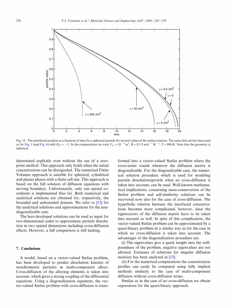
in Fig. 11 but now we use D12�/�/1�/D21 in Fig. 12.
Here the influence due to cross-diffusion is the same as
for the case where no surface tension is taken into
account. We note that surface tension is important for
growth of spherical particles, especially at the initial
stages of the growth process.
Of course for a spherical particle follows k�/1/S (t)
where S is the radius or interface position. The above
equation implies that the solubility product increases
when the particle radius decreases. This implies that the
interfacial (transformed) concentrations can become
such that a particle dissolves when the particle radius
is small and grows when its radius is large. This effect,
Ostwald-ripening, is well-known. Since our model is not
able to model ‘sub-critical’ growth we omit the compu-
tation of the growth kinetics of the particle, though later
stages of growth can be modeled by the use of the
present model.
To deal with cross-diffusion, we present an analytical
approach which can be used to determine easily the
influence of off-diagonal entries of the diffusion matrix.
We present an approach where dissolution times can be
Fig. 11. The interfacial position as a function of time for a spherical particle for several values of the surface tension. The same data set has been used
as for Fig. 1 (and Fig. 6) with D12�/0. In the computations we took Vm �/10�5 m3, R�/8.3 J mol�1 K�1, T�/800 K. Note that the geometry is
spherical.
F.J. Vermolen et al. / Materials Science and Engineering A347 (2003) 265�/279 277
determined explicitly even without the use of a zero-
point method. This approach only holds when the initial
concentrations can be disregarded. The numerical Finite
Volumes approach is suitable for spherical, cylindrical
and planar phases with a finite cell size. This approach isbased on the full solution of diffusion equations with
moving boundary. Unfortunately, only one spatial co-
ordinate is implemented thus far. Both numerical and
analytical solutions are obtained for, respectively, the
bounded and unbounded domain. We refer to [13] for
the analytical solutions and approximations for the non-
diagonalizable case.
The here developed solutions can be used as input fortwo-dimensional codes to approximate particle dissolu-
tion in two spatial dimensions including cross-diffusion
effects. However, a full comparison is still lacking.
7. Conclusions
A model, based on a vector-valued Stefan problem,
has been developed to predict dissolution kinetics of
stoichiometric particles in multi-component alloys.
Cross-diffusion of the alloying elements is taken intoaccount, which gives a strong coupling of the differential
equations. Using a diagonalization argument, the vec-
tor-valued Stefan problem with cross-diffusion is trans-
formed into a vector-valued Stefan problem where the
cross-terms vanish whenever the diffusion matrix is
diagonalizable. For the diagonalizable case, the numer-
ical solution procedure which is used for modeling
particle dissolution/growth when no cross-diffusion is
taken into account, can be used. Well-known mathema-
tical implications, concerning mass-conservation of the
Stefan problem and self-similarity solutions can be
recovered now also for the case of cross-diffusion. The
hyperbolic relation between the interfacial concentra-
tions becomes more complicated, however, since the
eigenvectors of the diffusion matrix have to be taken
into account as well. In spite of this complication, the
vector-valued Stefan problem can be approximated by a
quasi-binary problem in a similar way as for the case in
which no cross-diffusion is taken into account. The
advantages of the diagonalization procedure are.(i) The eigenvalues give a quick insight into the well-
posedness of the problem, negative eigenvalues are not
allowed. Existence of solutions for singular diffusion
matrices has been analyzed in [13].
(ii) For the numerical computations the concentration
profiles can easily be computed using fully implicit
methods similarly to the case of multi-component
diffusion without cross-diffusion terms.
Similar as in the case of no cross-diffusion we obtain
expressions for the quasi-binary approach.
Fig. 12. The interfacial position as a function of time for a spherical particle for several values of the surface tension. The same data set has been used
as for Fig. 1 (and Fig. 6) with D12�/�/1. In the computations we took Vm �/10�5 m3, R�/8.3 J mol�1 K�1, T�/800 K. Note that the geometry is
spherical.
F.J. Vermolen et al. / Materials Science and Engineering A347 (2003) 265�/279278

References
[1] M.J. Whelan, Metals Science Journal 3 (1969) 95�/97.
[2] F.V. Nolfi, Jr, P.G. Shewmon, J.S. Foster, Transactions of the
Metallurgical Society of AIME 245 (1969) 1427�/1433.
[3] O. Rciso, N. Ryum, J. Strid, Metallurgical Transactions A 24A
(1993) 2629�/2641.
[4] R. Hubcrt, ATB Metallurgie 34�/35 (1995) 4�/14.
[5] R. Kobayashi, Physics D 63 (1993) 410�/423.
[6] U. Grafe, B. Bottger, J. Tiadcn, S.G. Fries, Scripta Materialia 42
(12) (2000) 1179�/1186.
[7] G.B. Kalc, K. Bhanumurthy, S.K. Khera, M.K. Asundi, Materi-
als Transactions 32 (11) (1991) 1034�/1041.
[8] A. Vergara, L. Paduano, V. Vitagliano, R. Sartorio, Materials
Chemistry and Physics 66 (2000) 126�/131.
[9] K.P. Travis, K.E. Gubbins, Molecular Simulation 27 (5�/6) (2001)
405�/439.
[10] J.S. Kirkaldy, D.J. Young, Diffusion in the Condensed State, The
Institute of Metals, London, 1987.
[11] M.E. Glicksman, Diffusion in Solids, Wiley, New York, 2000.
[12] E.B. Naumann, J. Savoca, AICHE Journal 47 (5) (2001) 1016�/
1021.
[13] F.J. Vermolen, C. Vuik, S. van der Zwaag, Some mathematical
aspects of particle dissolution and cross-diffusion in multi-
component alloys, Delft University of Technology, 001, Depart-
ment of Applied Mathematical Analysis, see http://ta.twi.tu-
delft.nl/TWA-Reports/01-15.ps, 01-13, Delft, The Netherlands.
[14] F.J. Vermolen, C. Vuik, Journal of Computational and Applied
Mathematics 93 (1998) 123�/143.
[15] F.J. Vermolen, C. Vuik, Journal of Computational and Applied
Mathematics 126 (2001) 233�/254.
[16] F.J. Vermolen, C. Vuik, S. van der Zwaag, Materials Science and
Engineering A328 (2002) 14�/25.
[17] M. Farkas, Nonlinear Analysis, Theory, Methods and Applica-
tions 30 (1997) 1225�/1233.
[18] J. Crank, Free and Moving Boundary Problems, Clarendon Press,
Oxford, 1984.
[19] J. Chadam, H. Rasmusscn, Free Boundary Problems Involving
Solids, Longman, Scientific and Technical Harlow, 1993.
[20] A. Visintin, Models of Phase Transitions, Progress in Nonlinear
Differential Equations and their Application, vol. 38, Birkhauser,
Boston, 1996.
[21] G.H. Golub, C.P. van Loan, Matrix Computations, third ed., The
Johns Hopkins University Press, Baltimore, 1996.
[22] J.S. Kirkaldy, D. Weichert, Z.-U. Haq, Canadian Journal of
Physics 41 (1963) 2166�/2173.
[23] H.B. Aaron, G.R. Kotler, Metallurgical Transactions 2 (1971)
1651�/1656.
F.J. Vermolen et al. / Materials Science and Engineering A347 (2003) 265�/279 279