Embed Size (px)
Citation preview
Particle Image Segmentation Based on Bhattacharyya Distance
by
Dongmin Han
A Thesis Presented in Partial Fulfillment
of the Requirements for the Degree
Master of Science
Approved July 2015 by the
Graduate Supervisory Committee:
David Frakes, Chair
Ronald Adrian
Pavan Turaga
ARIZONA STATE UNIVERSITY
August 2015
i
ABSTRACT
Image segmentation is of great importance and value in many applications. In
computer vision, image segmentation is the tool and process of locating objects and
boundaries within images. The segmentation result may provide more meaningful image
data. Generally, there are two fundamental image segmentation algorithms: discontinuity
and similarity. The idea behind discontinuity is locating the abrupt changes in intensity of
images, as are often seen in edges or boundaries. Similarity subdivides an image into
regions that fit the pre-defined criteria. The algorithm utilized in this thesis is the second
category. [1]
This study addresses the problem of particle image segmentation by measuring the
similarity between a sampled region and an adjacent region, based on Bhattacharyya
distance and an image feature extraction technique that uses distribution of local binary
patterns and pattern contrasts. A boundary smoothing process is developed to improve the
accuracy of the segmentation. The novel particle image segmentation algorithm is tested
using four different cases of particle image velocimetry (PIV) images. The obtained
experimental results of segmentations provide partitioning of the objects within 10 percent
error rate. Ground-truth segmentation data, which are manually segmented image from
each case, are used to calculate the error rate of the segmentations.

ii
ACKNOWLEDGMENTS
I wish to thank my advisor Dr. David Frakes for his support and help on this
research project. I would like to thank my committee members Dr. Ronald Adrian and Dr.
Pavan Turaga for agreeing to be on my committee. I am also pleased to have this
opportunity to thank my colleagues Justin Ryan, Priya Nair and Berkay Kanberoglu for all
of their help.
Finally, I would like to thank my family for their support and encouragement.

iii
TABLE OF CONTENTS
Page
LIST OF TABLES ................................................................................................................... vi
LIST OF FIGURES ............................................................................................................... vii
CHAPTER
1 INTRODUCTION ............................................................................................................. 1
1.1 Motivation ...................................................................................................................... 1
1.1.1 Arterial Aneurysm .............................................................................................. 1
1.1.2 PIV System ......................................................................................................... 1
1.2 Relative Works ............................................................................................................... 2
1.2.1 Region Splitting and Merging ............................................................................ 2
1.2.2 Active Contour Model ........................................................................................ 3
1.2.3 Graph Cuts .......................................................................................................... 4
2 METHODS ........................................................................................................................ 6
2.1 Bhattacharyya Distance ................................................................................................. 6
2.2 Local Binary Pattern ...................................................................................................... 7
2.3 Sliding Neighborhood Operations ................................................................................. 8
2.4 Morphorlogical Image Processing ................................................................................. 9
2.4.1 Erosion and Dilation ........................................................................................... 9
2.4.2 Opening ............................................................................................................. 10
2.5 Boundary Following .................................................................................................... 11
2.6 Curvature of Plane Curves ........................................................................................... 12
3 PARTICLE IMAGE SEGMENTATION ....................................................................... 14

iv
CHAPTER Page
3.1 Preprocessing ............................................................................................................... 14
3.1.1 Image Padding .................................................................................................. 14
3.1.2 Image Adjusting ................................................................................................ 14
3.1.3 Threshold Setting .............................................................................................. 15
3.2 Combined Distance Image Calculation ....................................................................... 15
3.2.1 Selecting Sample Region and Creating The Histograms ................................. 15
3.2.2 Combined Distance Image ............................................................................... 17
3.3 Morphological Processing ........................................................................................... 20
3.4 Boundary Smoothing ................................................................................................... 22
4 RESULTS ....................................................................................................................... 24
4.1 Data Set Description .................................................................................................... 24
4.2 Segmentation Results ................................................................................................... 25
4.2.1 Results for the Case 1 ....................................................................................... 25
4.2.2 Results for the Case 2 ....................................................................................... 26
4.2.3 Results for the Case 3 ....................................................................................... 27
4.2.4 Results for the Case 4 ....................................................................................... 28
4.3 Analysis of the BC Method ......................................................................................... 29
4.4 Evaluation of the Algorithm Performance with Respect to the Ground-truth Data .. 31
4.5 Result for Boundary Smoothing and LBP Method ..................................................... 32
5 DISCUSSION ................................................................................................................. 35
5.1 Results Analysis ........................................................................................................... 35
5.2 Methods Analysis ......................................................................................................... 37

v
CHAPTER Page
5.2 Future Work ................................................................................................................. 37
6 CONCLUSION ............................................................................................................... 39
References ............................................................................................................................. 40

vi
LIST OF TABLES
Table Page
1. Error Rates, Combining Weights and Thresholds for for Four Cases ........................ 32
2. Error Rates Comparison for Boundary Smoothing...................................................... 33
3. Error Rates Comparison for LBP Method ................................................................... 34
vii
LIST OF FIGURES
Figure Page
1. Quadtree Splitting Technique ......................................................................................... 3
2. An Example of a Graph and a Cut ................................................................................. 5
3. Steps in the Calculation of LBP and C Value ............................................................... 8
4. Sliding Neighborhood Operation .................................................................................. 8
5. Example of Erosion ....................................................................................................... 9
6. Example of Dilation ..................................................................................................... 10
7. Example of Opening Operation ................................................................................... 11
8. Boundary Following .................................................................................................... 12
9. Boundary Following Steps .......................................................................................... 12
10. Image Padding ............................................................................................................. 14
11. Image Adjusting ........................................................................................................... 15
12. Sample Region Selecting ............................................................................................ 16
13. Unified Intensity Histograms....................................................................................... 17
14. BC Image ..................................................................................................................... 18
15. LBP/C Image ............................................................................................................... 19
16. Combined Distance Image .......................................................................................... 20
17. Binary Combined Distance Image .............................................................................. 21
18. Filled Combined Distance Image ................................................................................ 21
19. Open Operation Applied on Combined Distance Image ............................................ 22
20. Different Ways to Place the Points for Curvature Calculation ................................... 22
21. Four Particle Images Used for Testing ....................................................................... 25
viii
Figure Page
22. Results for Case 1 ........................................................................................................ 26
23. Results for Case 2 ........................................................................................................ 27
24. Results for Case 3 ........................................................................................................ 28
25. Results for Case 4 ........................................................................................................ 29
26. Sliding Window Positions and Sampled Region ........................................................ 30
27. Mean, Variance and BC Value Versus Sliding Distance ........................................... 31
28. Results Comparison for Boundary Smoothing ........................................................... 32
29. Results Comparison for LBP Method ......................................................................... 34
30. Sketches of Histograms of Sample Region and Non-particle Block ......................... 36
1
Chapter 1
INTRODUCTION
This chapter details the motivations behind this thesis and introduces some existing
work related to image segmentation techniques. Section 1.1 describes the motivations and
section 1.2 summarizes some relative works.
1.1 Motivation
1.1.1 Arterial Aneurysm
Although the precise mechanism for the formation of the arterial aneurysm is still
unknown, studies about aneurysms have been motivated by the need to clinically manage
the disease.
The human heart generates pulsatile flow that spreads through the network of
arteries. The components of the arterial wall have to continuously remodel and regenerate
to maintain proper function and accommodate for the perpetual periodic stresses. However,
a lesion can develop at a weakening of an arterial wall. The pressure pushes outwards, and
creates a bulge area on the arterial wall. This weakening is an arterial aneurysm. [2]
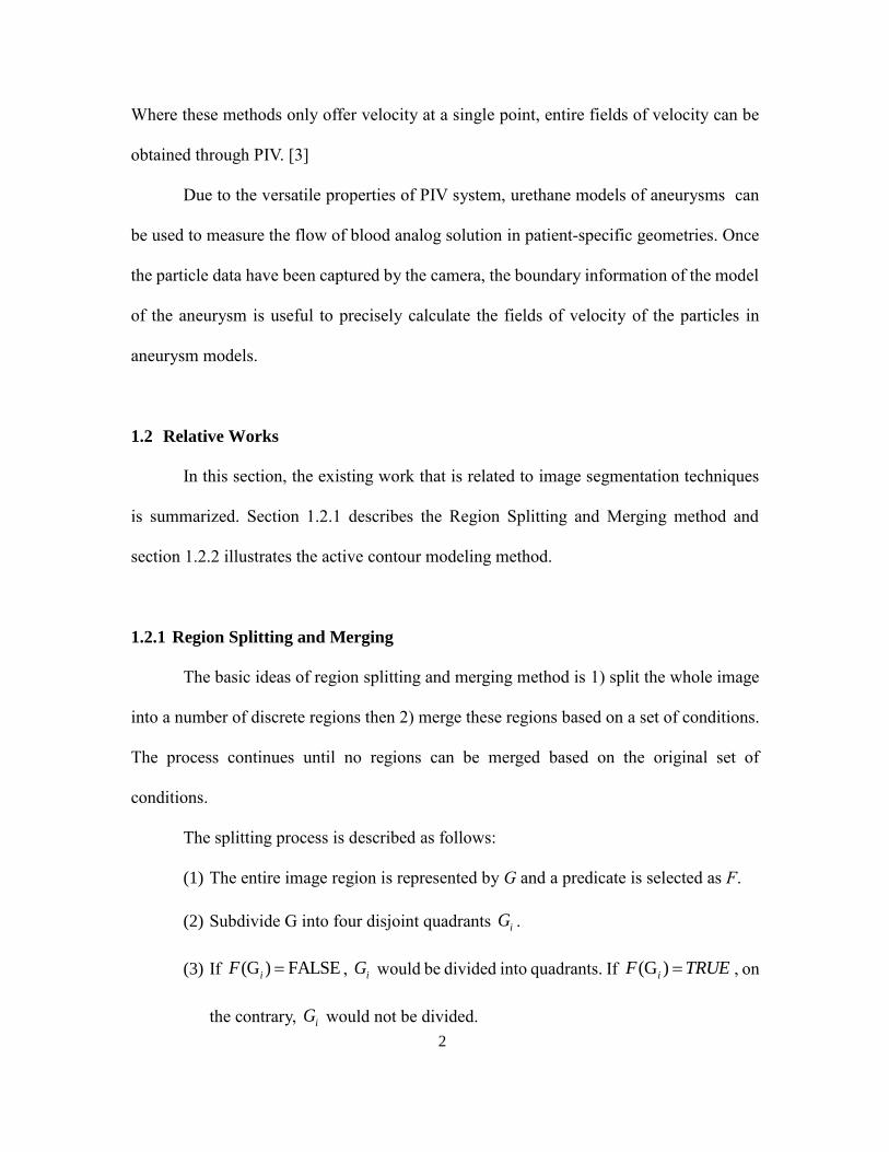
1.1.2 PIV System
Particle image velocimetry (PIV) is used to describe the instantaneous velocity
fields by measuring the movement of particles that follow the fluid flow.
PIV can be used to directly derive the velocity by measuring particle displacement
over time. Unlike other velocity measurement methods, which measure an intermediate
physical variables such as scalar image velocimetry and image correlation velocometry.
2
Where these methods only offer velocity at a single point, entire fields of velocity can be
obtained through PIV. [3]
Due to the versatile properties of PIV system, urethane models of aneurysms can
be used to measure the flow of blood analog solution in patient-specific geometries. Once
the particle data have been captured by the camera, the boundary information of the model
of the aneurysm is useful to precisely calculate the fields of velocity of the particles in
aneurysm models.
1.2 Relative Works
In this section, the existing work that is related to image segmentation techniques
is summarized. Section 1.2.1 describes the Region Splitting and Merging method and
section 1.2.2 illustrates the active contour modeling method.
1.2.1 Region Splitting and Merging
The basic ideas of region splitting and merging method is 1) split the whole image
into a number of discrete regions then 2) merge these regions based on a set of conditions.
The process continues until no regions can be merged based on the original set of
conditions.
The splitting process is described as follows:
(1) The entire image region is represented by G and a predicate is selected as F.
(2) Subdivide G into four disjoint quadrants iG .
(3) If (G ) FALSEiF , iG would be divided into quadrants. If (G )iF TRUE , on
the contrary, iG would not be divided.
3
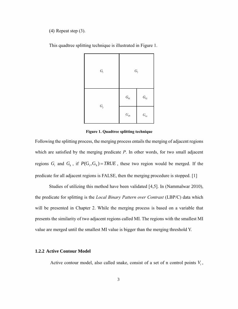
(4) Repeat step (3).
This quadtree splitting technique is illustrated in Figure 1.
Figure 1. Quadtree splitting technique
Following the splitting process, the merging process entails the merging of adjacent regions
which are satisfied by the merging predicate P. In other words, for two small adjacent
regions iG and kG , if (G ,G )i kP TRUE , these two region would be merged. If the
predicate for all adjacent regions is FALSE, then the merging procedure is stopped. [1]
Studies of utilizing this method have been validated [4,5]. In (Nammalwar 2010),
the predicate for splitting is the Local Binary Pattern over Contrast (LBP/C) data which
will be presented in Chapter 2. While the merging process is based on a variable that
presents the similarity of two adjacent regions called MI. The regions with the smallest MI
value are merged until the smallest MI value is bigger than the merging threshold Y.
1.2.2 Active Contour Model
Active contour model, also called snake, consist of a set of n control points iV ,
4
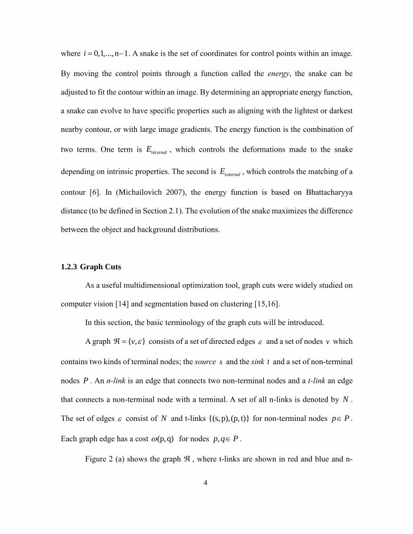
where 0,1,...,n 1i . A snake is the set of coordinates for control points within an image.
By moving the control points through a function called the energy, the snake can be
adjusted to fit the contour within an image. By determining an appropriate energy function,
a snake can evolve to have specific properties such as aligning with the lightest or darkest
nearby contour, or with large image gradients. The energy function is the combination of
two terms. One term is internalE , which controls the deformations made to the snake
depending on intrinsic properties. The second is externalE , which controls the matching of a
contour [6]. In (Michailovich 2007), the energy function is based on Bhattacharyya
distance (to be defined in Section 2.1). The evolution of the snake maximizes the difference
between the object and background distributions.
1.2.3 Graph Cuts
As a useful multidimensional optimization tool, graph cuts were widely studied on
computer vision [14] and segmentation based on clustering [15,16].
In this section, the basic terminology of the graph cuts will be introduced.
A graph { , }v consists of a set of directed edges and a set of nodes v which
contains two kinds of terminal nodes; the source s and the sink t and a set of non-terminal
nodes P . An n-link is an edge that connects two non-terminal nodes and a t-link an edge
that connects a non-terminal node with a terminal. A set of all n-links is denoted by N .
The set of edges consist of N and t-links {(s,p),(p, t)} for non-terminal nodes p P .
Each graph edge has a cost (p,q) for nodes ,p q P .
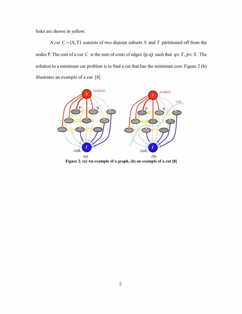
Figure 2 (a) shows the graph , where t-links are shown in red and blue and n-
5
links are shown in yellow.
A cut {S,T}C consists of two disjoint subsets S and T partitioned off from the
nodes P. The cost of a cut C is the sum of costs of edges (p,q) such that ,q T p S . The
solution to a minimum cut problem is to find a cut that has the minimum cost. Figure 2 (b)
illustrates an example of a cut. [8]
(a) (b)
Figure 2. (a) An example of a graph, (b) an example of a cut [8]
6
Chapter 2
METHODS
This chapter introduces some background knowledge on imaging processing
especially regarding imaging segmentation. In section 2.1, the statistic method,
Bhattacharyya distance is described. In section 2.2, some basic morphological image
processing are illustrated for further use. The procedures of boundary following are
introduced in section 2.3. In section 2.4, calculation of curvature of plane curves is
described.
2.1 Bhattacharyya Distance
Bhattacharyya Distance is the measurement between two probability distributions.
The definition of Bhattacharyya Distance is:
1 2( , ) -ln ( , )Bhattacharyyad H H BC p q , (1)
where:
( , ) ( ) ( )x X
BC p q p x q x
. (2)
is the Bhattacharyya coefficient (BC). (x)p and (x)q are the two normalized
distributions.
For Bhattacharyya distance, a higher value indicates a better match between two
distributions. The value or distance of a total mismatch is 1, and a perfect match is 0. The
histograms of images must be normalized before comparing so that the size of the image
will not impact the distance. [9]
7
2.2 Local Binary Pattern
One of the most useful ways to segment a PIV image is to extract the texture feature
from the region containing particles. Local Binary Pattern (LBP) [10] is one of the
techniques used to extract the local texture feature, which is based on possible value sets
called texture units (TU) that is obtained from each pixel. A TU is an eight elements set
1 2 8{ , ,..., ,}TU E E E , which represents the possible values (0, 1) of the neighborhood of
3-by-3 pixels 0 1 8{ , ,..., ,}V V V V , in which 0V is the central pixel. The values of TU is
obtained by the following rule:
0
0
0
1
i
i
i
V VE
V V
. (3)
LBP is represented by the equation:
81
1
2i
i
i
LBP E
. (4)
This LBP value can only describe the “direction” of the local texture, which is not enough
to indicate the texture patterns that also contains the gray scale variations. So the contrast
of the texture (C) is combined with the LBP value to represent the local texture pattern of
the image. The contrast is represented by the difference between the average intensity
values of pixels corresponding to the value 0 and 1 in the TU. A 256-bin histogram, which
is represented by the distribution of the LBP/C of the image, describes the texture spectrum
of an 8-bit image. The following is an example of what is mentioned above for one central
pixel:
8
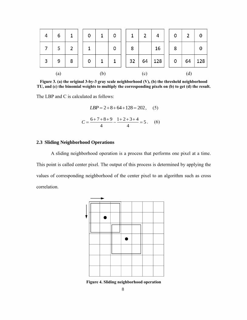
(a) (b) (c) (d)
Figure 3. (a) the original 3-by-3 gray scale neighborhood (V), (b) the thresheld neighborhood
TU, and (c) the binomial weights to multiply the corresponding pixels on (b) to get (d) the result.
The LBP and C is calculated as follows:
2 8 64 128 202LBP , (5)
6 7 8 9 1 2 3 4
54 4
C
. (6)
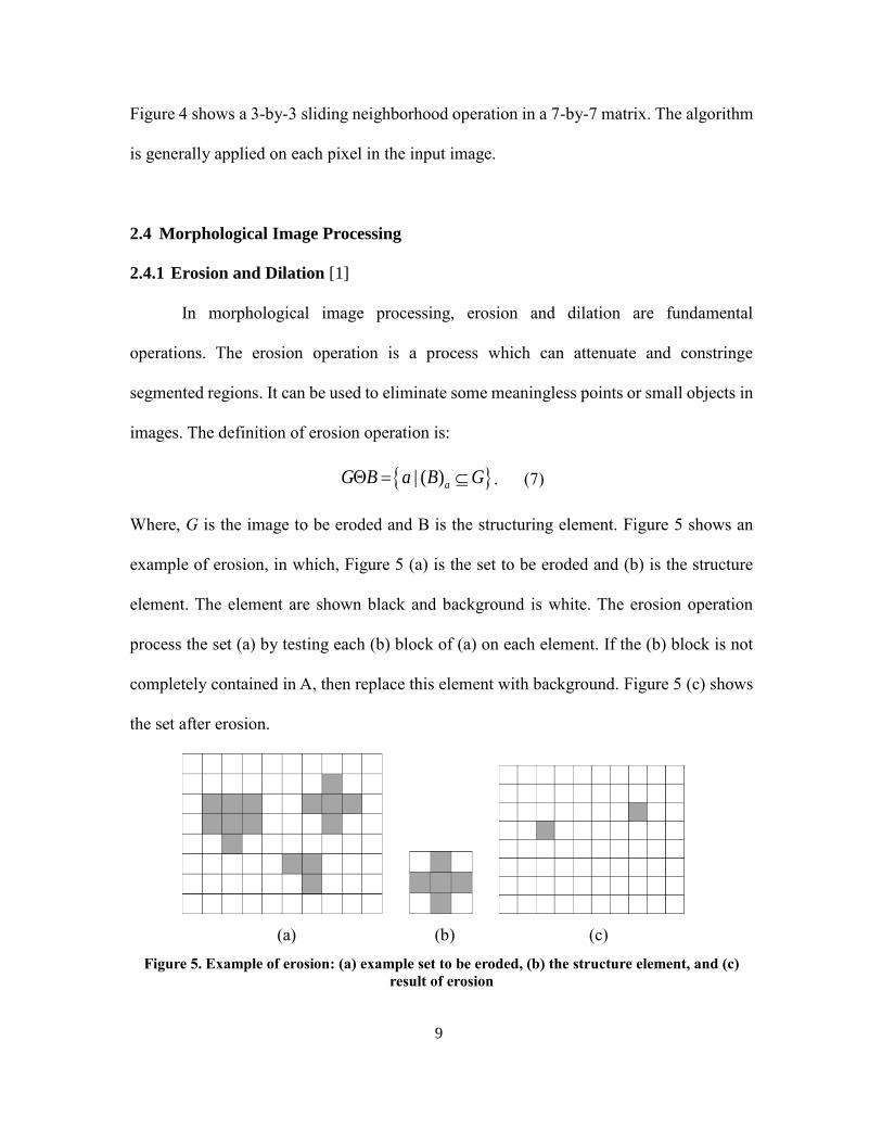
2.3 Sliding Neighborhood Operations
A sliding neighborhood operation is a process that performs one pixel at a time.
This point is called center pixel. The output of this process is determined by applying the
values of corresponding neighborhood of the center pixel to an algorithm such as cross
correlation.
Figure 4. Sliding neighborhood operation
9
Figure 4 shows a 3-by-3 sliding neighborhood operation in a 7-by-7 matrix. The algorithm
is generally applied on each pixel in the input image.
2.4 Morphological Image Processing
2.4.1 Erosion and Dilation [1]
In morphological image processing, erosion and dilation are fundamental
operations. The erosion operation is a process which can attenuate and constringe
segmented regions. It can be used to eliminate some meaningless points or small objects in
images. The definition of erosion operation is:
| ( )aG B a B G . (7)
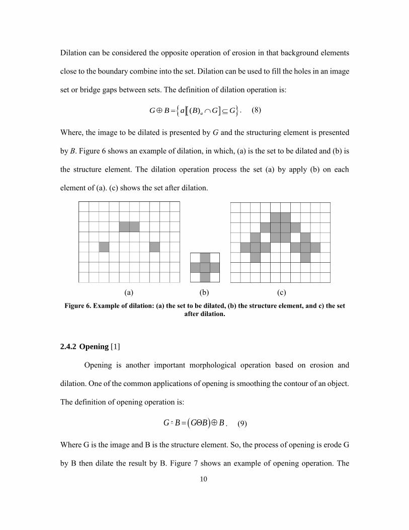
Where, G is the image to be eroded and B is the structuring element. Figure 5 shows an
example of erosion, in which, Figure 5 (a) is the set to be eroded and (b) is the structure
element. The element are shown black and background is white. The erosion operation
process the set (a) by testing each (b) block of (a) on each element. If the (b) block is not
completely contained in A, then replace this element with background. Figure 5 (c) shows
the set after erosion.
(a) (b) (c)
Figure 5. Example of erosion: (a) example set to be eroded, (b) the structure element, and (c)
result of erosion
10
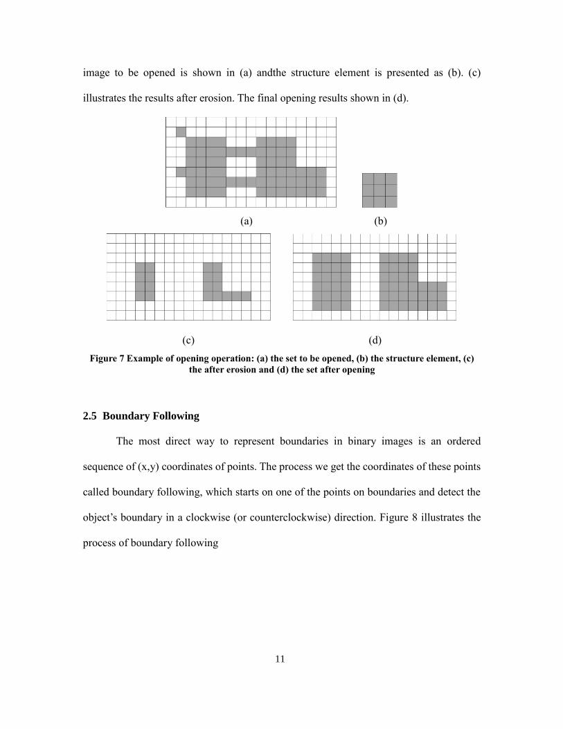
Dilation can be considered the opposite operation of erosion in that background elements
close to the boundary combine into the set. Dilation can be used to fill the holes in an image
set or bridge gaps between sets. The definition of dilation operation is:
( )aG B a B G G . (8)
Where, the image to be dilated is presented by G and the structuring element is presented
by B. Figure 6 shows an example of dilation, in which, (a) is the set to be dilated and (b) is
the structure element. The dilation operation process the set (a) by apply (b) on each
element of (a). (c) shows the set after dilation.
(a) (b) (c)
Figure 6. Example of dilation: (a) the set to be dilated, (b) the structure element, and c) the set
after dilation.
2.4.2 Opening [1]
Opening is another important morphological operation based on erosion and
dilation. One of the common applications of opening is smoothing the contour of an object.
The definition of opening operation is:
G B G B B . (9)
Where G is the image and B is the structure element. So, the process of opening is erode G
by B then dilate the result by B. Figure 7 shows an example of opening operation. The
11
image to be opened is shown in (a) andthe structure element is presented as (b). (c)
illustrates the results after erosion. The final opening results shown in (d).
(a) (b)
(c) (d)
Figure 7 Example of opening operation: (a) the set to be opened, (b) the structure element, (c)
the after erosion and (d) the set after opening
2.5 Boundary Following
The most direct way to represent boundaries in binary images is an ordered
sequence of (x,y) coordinates of points. The process we get the coordinates of these points
called boundary following, which starts on one of the points on boundaries and detect the
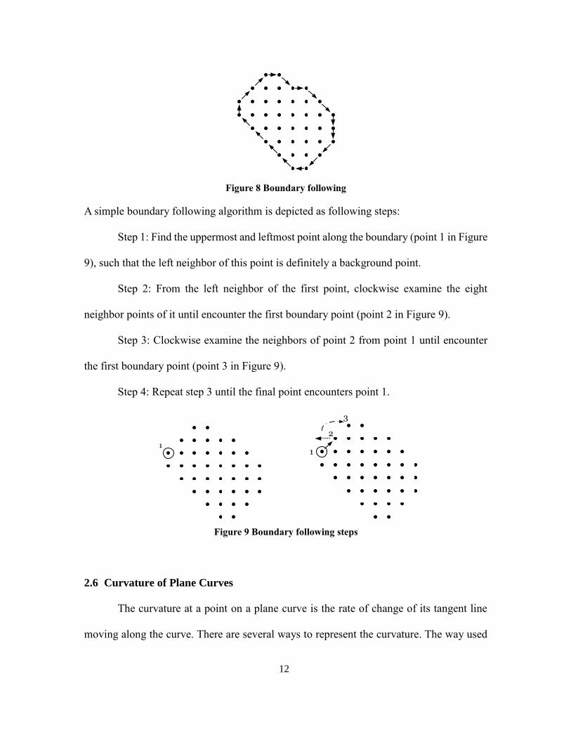
object’s boundary in a clockwise (or counterclockwise) direction. Figure 8 illustrates the
process of boundary following
12
Figure 8 Boundary following
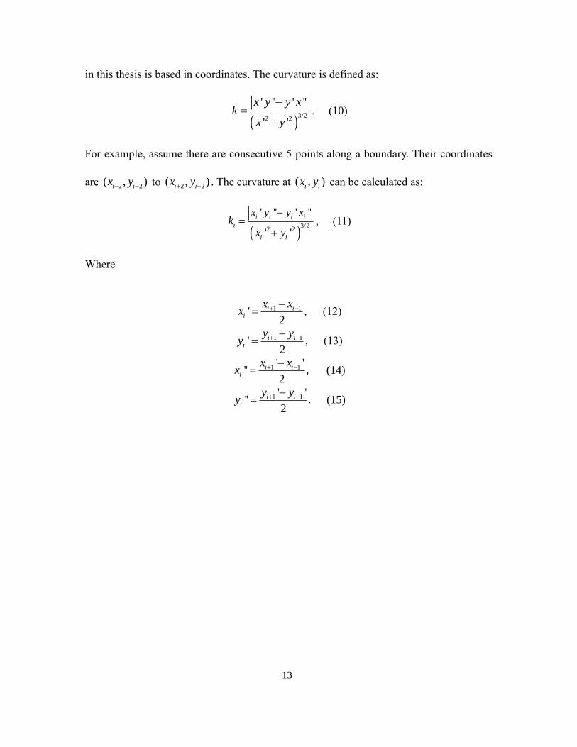
A simple boundary following algorithm is depicted as following steps:
Step 1: Find the uppermost and leftmost point along the boundary (point 1 in Figure
9), such that the left neighbor of this point is definitely a background point.
Step 2: From the left neighbor of the first point, clockwise examine the eight
neighbor points of it until encounter the first boundary point (point 2 in Figure 9).
Step 3: Clockwise examine the neighbors of point 2 from point 1 until encounter
the first boundary point (point 3 in Figure 9).
Step 4: Repeat step 3 until the final point encounters point 1.
1
1
2
3
Figure 9 Boundary following steps
2.6 Curvature of Plane Curves
The curvature at a point on a plane curve is the rate of change of its tangent line
moving along the curve. There are several ways to represent the curvature. The way used
13
in this thesis is based in coordinates. The curvature is defined as:
3/2
2 2
' '' ' ''
' '
x y y xk
x y
. (10)
For example, assume there are consecutive 5 points along a boundary. Their coordinates
are 2 2( , )i ix y to 2 2( , )i ix y . The curvature at ( , )i ix y can be calculated as:
3/2
2 2
' '' ' ''
' '
i i i i
i
i i
x y y xk
x y
, (11)
Where
1 1' ,2
i ii
x xx
(12)
1 1' ,2
i ii
y yy
(13)
1 1' ''' ,
2
i ii
x xx
(14)
1 1' ''' .
2
i ii
y yy
(15)
14
Chapter 3
PARTICLE IMAGE SEGMENTATION
This chapter introduces the implemented procedure of particle image segmentation.
There are four major steps in the image segmentation process: 1) image preprocessing
which consists image padding and threshold setting, 2) calculating the Bhattacharyya
distance image, 3) morphological processing and boundary describing, and 4) boundary
smoothing.
3.1 Preprocessing
3.1.1 Image Padding
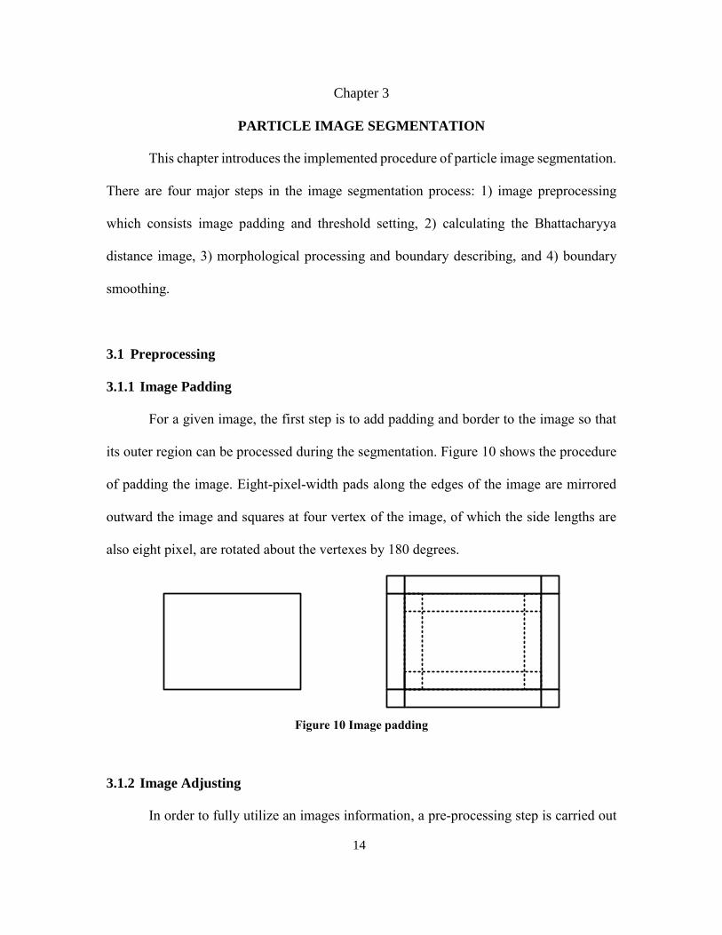
For a given image, the first step is to add padding and border to the image so that
its outer region can be processed during the segmentation. Figure 10 shows the procedure
of padding the image. Eight-pixel-width pads along the edges of the image are mirrored
outward the image and squares at four vertex of the image, of which the side lengths are
also eight pixel, are rotated about the vertexes by 180 degrees.
Figure 10 Image padding
3.1.2 Image Adjusting
In order to fully utilize an images information, a pre-processing step is carried out
15
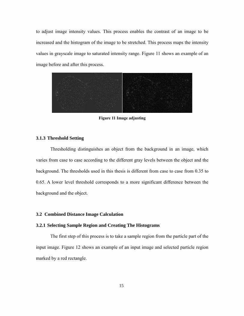
to adjust image intensity values. This process enables the contrast of an image to be
increased and the histogram of the image to be stretched. This process maps the intensity
values in grayscale image to saturated intensity range. Figure 11 shows an example of an
image before and after this process.
Figure 11 Image adjusting
3.1.3 Threshold Setting
Thresholding distinguishes an object from the background in an image, which
varies from case to case according to the different gray levels between the object and the
background. The thresholds used in this thesis is different from case to case from 0.35 to
0.65. A lower level threshold corresponds to a more significant difference between the
background and the object.
3.2 Combined Distance Image Calculation
3.2.1 Selecting Sample Region and Creating The Histograms
The first step of this process is to take a sample region from the particle part of the
input image. Figure 12 shows an example of an input image and selected particle region
marked by a red rectangle.
16
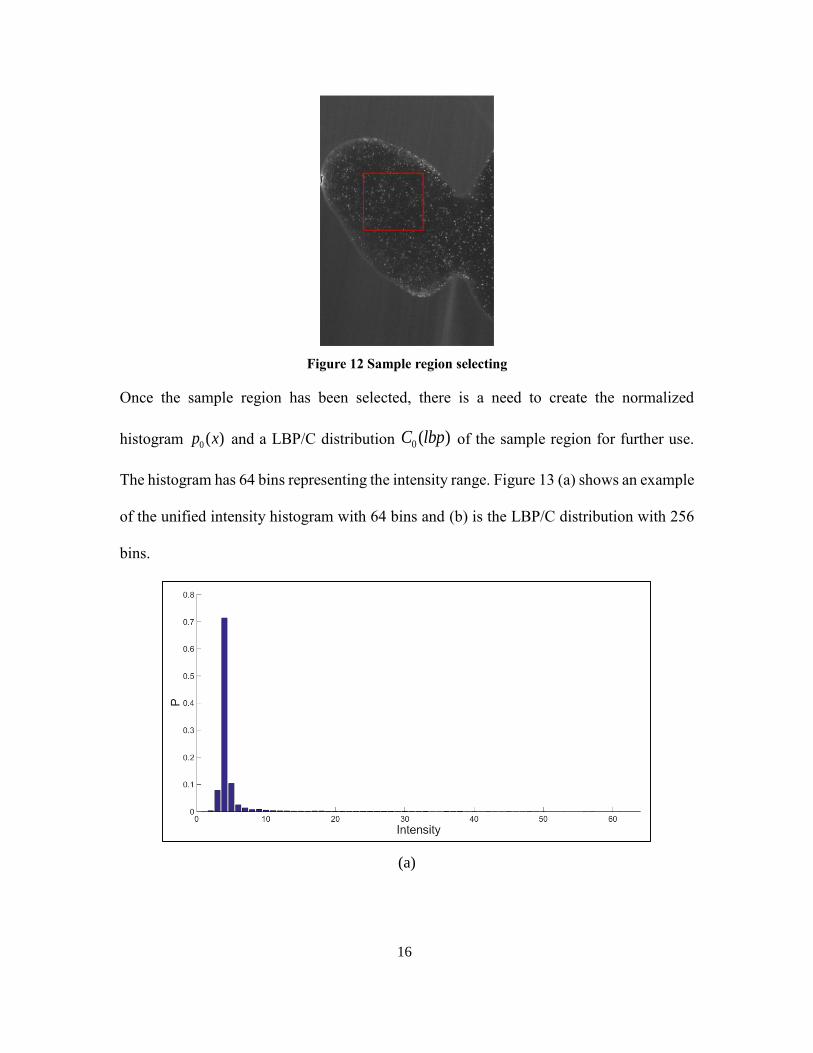
Figure 12 Sample region selecting
Once the sample region has been selected, there is a need to create the normalized
histogram 0 ( )p x and a LBP/C distribution 0 ( )C lbp of the sample region for further use.
The histogram has 64 bins representing the intensity range. Figure 13 (a) shows an example
of the unified intensity histogram with 64 bins and (b) is the LBP/C distribution with 256
bins.
(a)
17
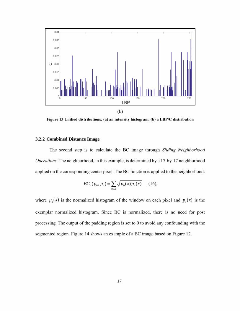
(b)
Figure 13 Unified distributions: (a) an intensity histogram, (b) a LBP/C distribution
3.2.2 Combined Distance Image
The second step is to calculate the BC image through Sliding Neighborhood
Operations. The neighborhood, in this example, is determined by a 17-by-17 neighborhood
applied on the corresponding center pixel. The BC function is applied to the neighborhood:
0 0( , ) ( ) ( )n n n
x X
BC p p p x p x
(16),
where ( )np x is the normalized histogram of the window on each pixel and 0 ( )p x is the
exemplar normalized histogram. Since BC is normalized, there is no need for post
processing. The output of the padding region is set to 0 to avoid any confounding with the
segmented region. Figure 14 shows an example of a BC image based on Figure 12.
18
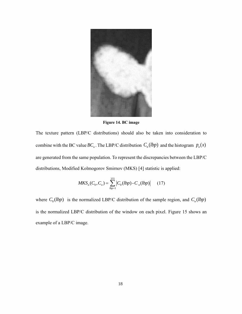
Figure 14. BC image
The texture pattern (LBP/C distributions) should also be taken into consideration to
combine with the BC value nBC . The LBP/C distribution ( )nC lbp and the histogram ( )np x
are generated from the same population. To represent the discrepancies between the LBP/C
distributions, Modified Kolmogorov Smirnov (MKS) [4] statistic is applied:
255
0 0
1
( , ) ( ) - ( )n n n
lbp
MKS C C C lbp C lbp
(17)
where 0 ( )C lbp is the normalized LBP/C distribution of the sample region, and ( )nC lbp
is the normalized LBP/C distribution of the window on each pixel. Figure 15 shows an
example of a LBP/C image.
19
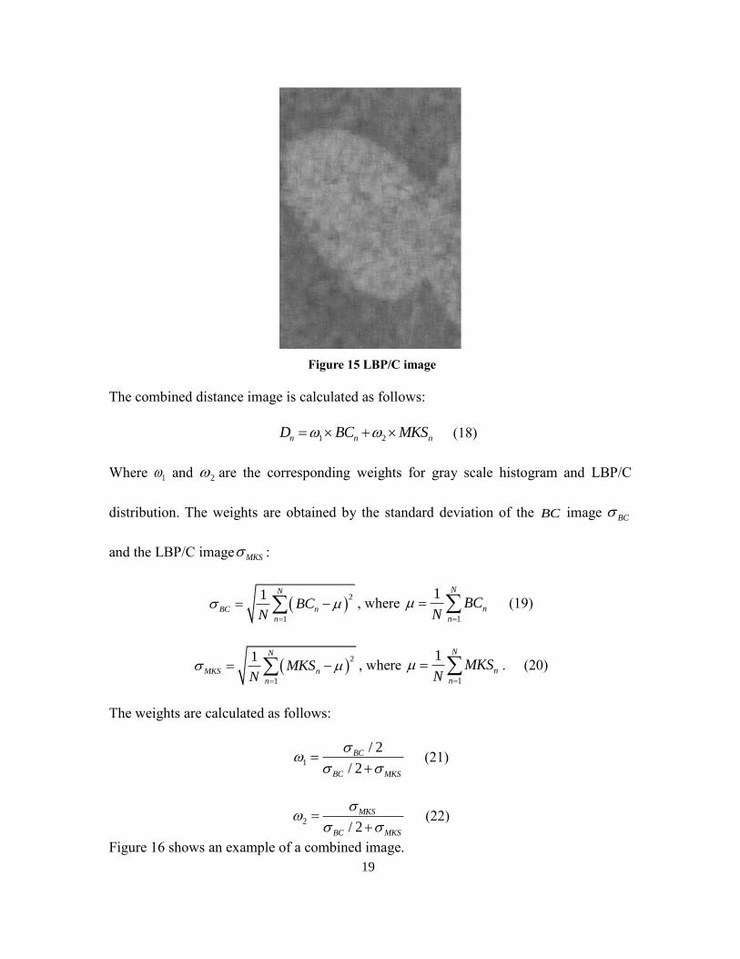
Figure 15 LBP/C image
The combined distance image is calculated as follows:
1 2n n nD BC MKS (18)
Where 1 and 2 are the corresponding weights for gray scale histogram and LBP/C
distribution. The weights are obtained by the standard deviation of the BC image BC
and the LBP/C image MKS :
2
1
1 N
BC n
n
BCN
, where 1
1 N
n
n
BCN
(19)
2
1
1 N
MKS n
n
MKSN
, where 1
1 N
n
n
MKSN
. (20)
The weights are calculated as follows:
1
/ 2
/ 2
BC
BC MKS
(21)
2/ 2
MKS
BC MKS
(22)
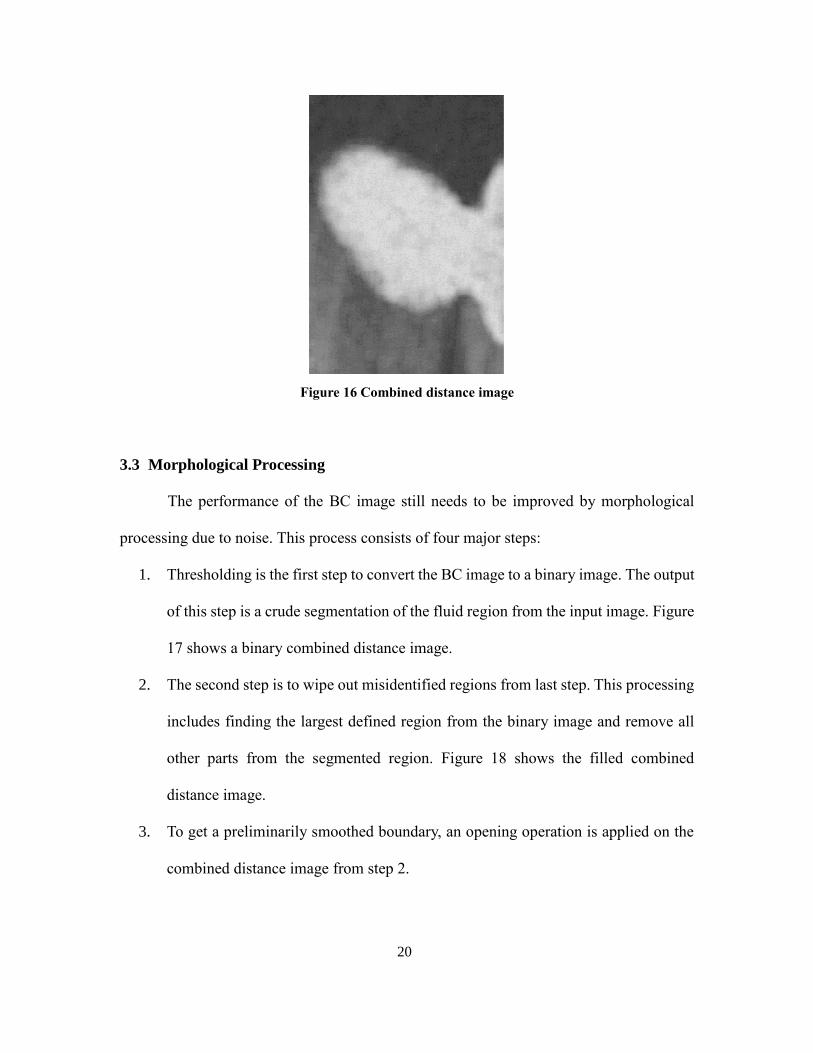
Figure 16 shows an example of a combined image.
20
Figure 16 Combined distance image
3.3 Morphological Processing
The performance of the BC image still needs to be improved by morphological
processing due to noise. This process consists of four major steps:
1. Thresholding is the first step to convert the BC image to a binary image. The output
of this step is a crude segmentation of the fluid region from the input image. Figure
17 shows a binary combined distance image.
2. The second step is to wipe out misidentified regions from last step. This processing
includes finding the largest defined region from the binary image and remove all
other parts from the segmented region. Figure 18 shows the filled combined
distance image.
3. To get a preliminarily smoothed boundary, an opening operation is applied on the
combined distance image from step 2.

21
Figure 17 Binary combined distance image
4. Once the opening processing has been applied, step 2 should be repeated as step 3
may cause some small parts to be separated from the main defined region.
Figure 18 Filled combined distance image
Figure 19 shows the difference between a part of an original contour and the one
that has been opened.
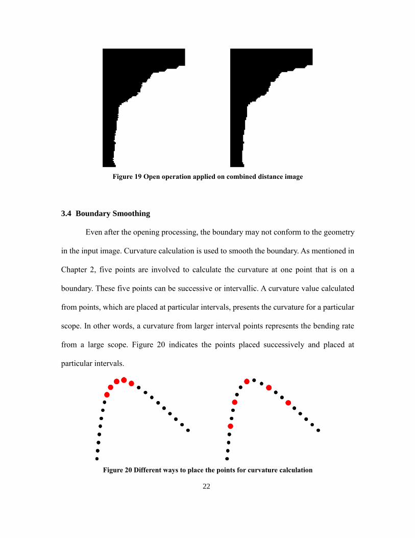
22
Figure 19 Open operation applied on combined distance image
3.4 Boundary Smoothing
Even after the opening processing, the boundary may not conform to the geometry
in the input image. Curvature calculation is used to smooth the boundary. As mentioned in
Chapter 2, five points are involved to calculate the curvature at one point that is on a
boundary. These five points can be successive or intervallic. A curvature value calculated
from points, which are placed at particular intervals, presents the curvature for a particular
scope. In other words, a curvature from larger interval points represents the bending rate
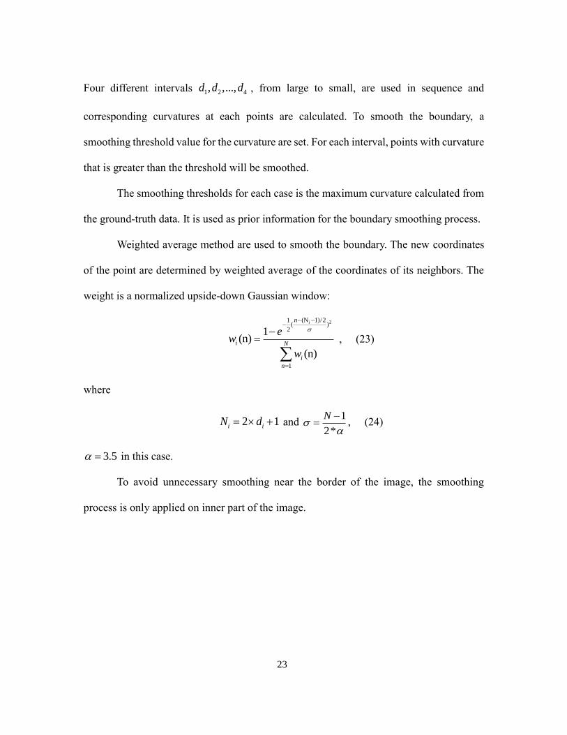
from a large scope. Figure 20 indicates the points placed successively and placed at
particular intervals.
Figure 20 Different ways to place the points for curvature calculation
23
Four different intervals 1 2 4, ,...,d d d , from large to small, are used in sequence and
corresponding curvatures at each points are calculated. To smooth the boundary, a
smoothing threshold value for the curvature are set. For each interval, points with curvature
that is greater than the threshold will be smoothed.
The smoothing thresholds for each case is the maximum curvature calculated from
the ground-truth data. It is used as prior information for the boundary smoothing process.
Weighted average method are used to smooth the boundary. The new coordinates
of the point are determined by weighted average of the coordinates of its neighbors. The
weight is a normalized upside-down Gaussian window:
2(N 1)/21( )
2
1
1(n)
(n)
in
i N
i
n
ew
w
, (23)
where
2 1i iN d and 1
2*
N
, (24)
3.5 in this case.
To avoid unnecessary smoothing near the border of the image, the smoothing
process is only applied on inner part of the image.
24
Chapter 4
RESULTS
In this chapter, the experimental results of the particle image segmentation using
different images sets are presented and analyzed utilizing the image processing steps as
described in Chapter 3. Section 4.1 illustrates the image sets used to evaluate the
performance of the combined distance segmentation algorithm. Section 4.2 represents the
performance of the algorithm. Section 4.3 evaluates the performance of the algorithm by
compare the segmentation results with the truth-ground. Section 4.4 specifies the results of
the smoothing process.
4.1 Data Set Description
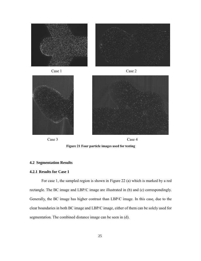
To test the combined distance segmentation, four different particle image sets are
used and shown in Figure 21. The four cases are PIV data captured using CCD cameras. A
blood analog solution, which contains a mixture of sodium iodide, glycerin and water, is
seeded with 8 µm fluorescent polymer microspheres and passes through an optically clear,
lost-core urethane model of the aneurysm. The fluid flowing through the model is
illuminated by a laser light sheet that excites the fluorescent particles. The blood analog
solution’s refractive index is matched with urethane to avoid optical distortions. [11]
25
Case 1 Case 2
Case 3 Case 4
Figure 21 Four particle images used for testing
4.2 Segmentation Results
4.2.1 Results for Case 1
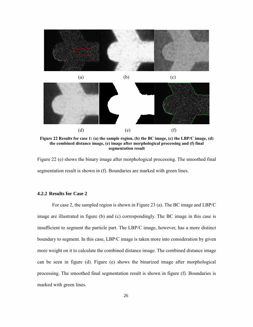
For case 1, the sampled region is shown in Figure 22 (a) which is marked by a red
rectangle. The BC image and LBP/C image are illustrated in (b) and (c) correspondingly.
Generally, the BC image has higher contrast than LBP/C image. In this case, due to the
clear boundaries in both BC image and LBP/C image, either of them can be solely used for
segmentation. The combined distance image can be seen in (d).
26
(a) (b) (c)
(d) (e) (f)
Figure 22 Results for case 1: (a) the sample region, (b) the BC image, (c) the LBP/C image, (d)
the combined distance image, (e) image after morphological processing and (f) final
segmentation result
Figure 22 (e) shows the binary image after morphological processing. The smoothed final
segmentation result is shown in (f). Boundaries are marked with green lines.
4.2.2 Results for Case 2
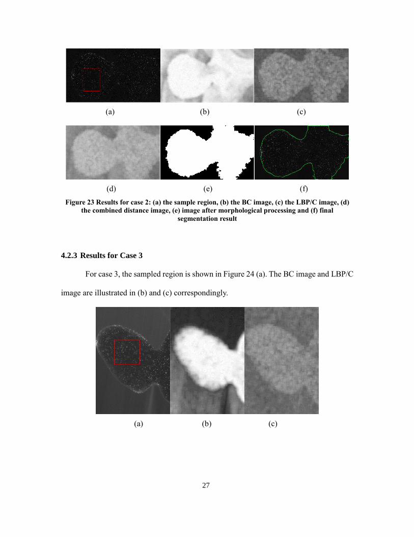
For case 2, the sampled region is shown in Figure 23 (a). The BC image and LBP/C
image are illustrated in figure (b) and (c) correspondingly. The BC image in this case is
insufficient to segment the particle part. The LBP/C image, however, has a more distinct
boundary to segment. In this case, LBP/C image is taken more into consideration by given
more weight on it to calculate the combined distance image. The combined distance image
can be seen in figure (d). Figure (e) shows the binarized image after morphological
processing. The smoothed final segmentation result is shown in figure (f). Boundaries is
marked with green lines.
27
(a) (b) (c)
(d) (e) (f)
Figure 23 Results for case 2: (a) the sample region, (b) the BC image, (c) the LBP/C image, (d)
the combined distance image, (e) image after morphological processing and (f) final
segmentation result
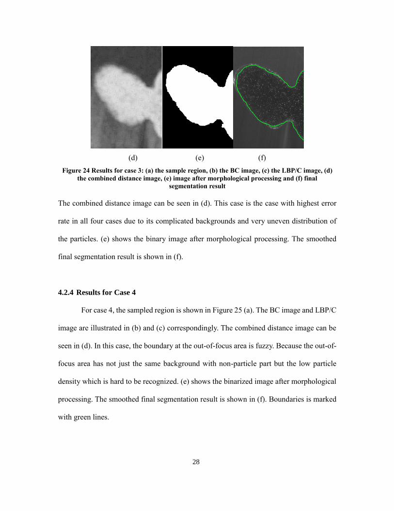
4.2.3 Results for Case 3
For case 3, the sampled region is shown in Figure 24 (a). The BC image and LBP/C
image are illustrated in (b) and (c) correspondingly.
(a) (b) (c)
28
(d) (e) (f)
Figure 24 Results for case 3: (a) the sample region, (b) the BC image, (c) the LBP/C image, (d)
the combined distance image, (e) image after morphological processing and (f) final
segmentation result
The combined distance image can be seen in (d). This case is the case with highest error
rate in all four cases due to its complicated backgrounds and very uneven distribution of
the particles. (e) shows the binary image after morphological processing. The smoothed
final segmentation result is shown in (f).
4.2.4 Results for Case 4
For case 4, the sampled region is shown in Figure 25 (a). The BC image and LBP/C
image are illustrated in (b) and (c) correspondingly. The combined distance image can be
seen in (d). In this case, the boundary at the out-of-focus area is fuzzy. Because the out-of-
focus area has not just the same background with non-particle part but the low particle
density which is hard to be recognized. (e) shows the binarized image after morphological
processing. The smoothed final segmentation result is shown in (f). Boundaries is marked
with green lines.

29
(a) (b) (c)
(d) (e) (f)
Figure 25 Results for case 4: (a) the sample region, (b) the BC image, (c) the LBP/C image, (d)
the combined distance image, (e) image after morphological processing and (f) final
segmentation result
4.3 Analysis of the BC Method
To evaluate the BC method. A sliding window test is arranged on a real case of
particle image, which is Case 1 in Section 4.1.
In this test, the 31×31 window slides from the non-particle part into the particle
part. In Figure 26, the white rectangle indicates the starting position of the sliding window
and the green rectangle indicates the ending position. The red rectangle declares the
sampled region that used to calculate the BC.
30
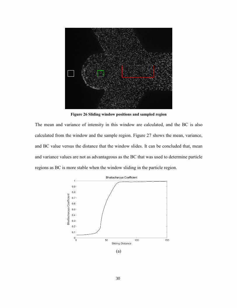
Figure 26 Sliding window positions and sampled region
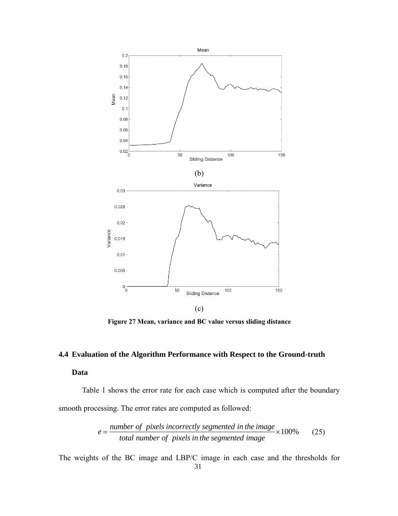
The mean and variance of intensity in this window are calculated, and the BC is also
calculated from the window and the sample region. Figure 27 shows the mean, variance,
and BC value versus the distance that the window slides. It can be concluded that, mean
and variance values are not as advantageous as the BC that was used to determine particle
regions as BC is more stable when the window sliding in the particle region.
(a)
31
(b)
(c)
Figure 27 Mean, variance and BC value versus sliding distance
4.4 Evaluation of the Algorithm Performance with Respect to the Ground-truth
Data
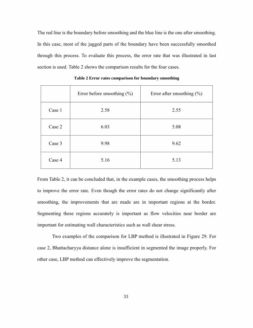
Table 1 shows the error rate for each case which is computed after the boundary
smooth processing. The error rates are computed as followed:
100%number of pixels incorrectly segmented in the image
etotal number of pixels in the segmented image
(25)
The weights of the BC image and LBP/C image in each case and the thresholds for
32
segmentation is also shown in the table. 1 is the weight for BC image and 2 is for
LBP/C image.
Error rate
(%) 1 2 Threshold
Smoothing
Threshold
Case 1 2.55 0.61 0.39 0.65 0.13
Case 2 5.08 0.4 0.6 0.6 0.03
Case 3 9.62 0.69 0.31 0.48 0.05
Case 4 5.13 0.67 0.33 0.35 0.05
Table 1 Error rates, combining weights and thresholds for four cases
4.5 Result for Boundary Smoothing and LBP Method
In this section, the comparisons between results of the segmentation with and
without the boundary smoothing, and between results with and without LBP method are
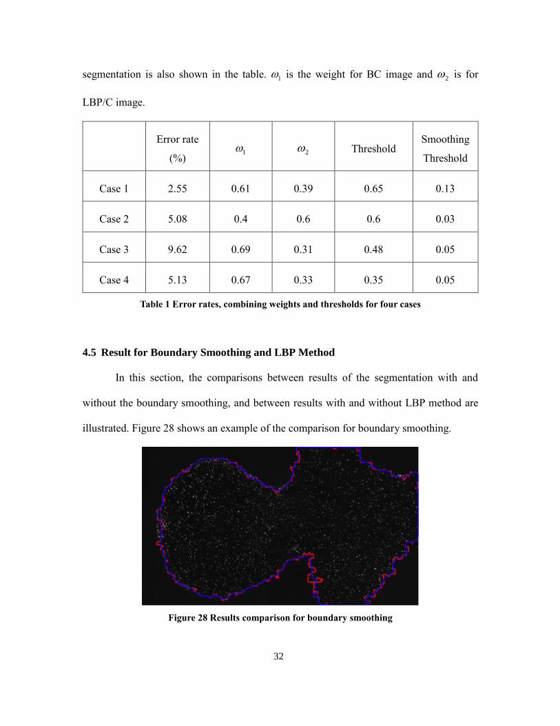
illustrated. Figure 28 shows an example of the comparison for boundary smoothing.
Figure 28 Results comparison for boundary smoothing
33
The red line is the boundary before smoothing and the blue line is the one after smoothing.
In this case, most of the jagged parts of the boundary have been successfully smoothed
through this process. To evaluate this process, the error rate that was illustrated in last
section is used. Table 2 shows the comparison results for the four cases.
Table 2 Error rates comparison for boundary smoothing
Error before smoothing (%) Error after smoothing (%)
Case 1 2.58 2.55
Case 2 6.03 5.08
Case 3 9.98 9.62
Case 4 5.16 5.13
From Table 2, it can be concluded that, in the example cases, the smoothing process helps
to improve the error rate. Even though the error rates do not change significantly after
smoothing, the improvements that are made are in important regions at the border.
Segmenting these regions accurately is important as flow velocities near border are
important for estimating wall characteristics such as wall shear stress.
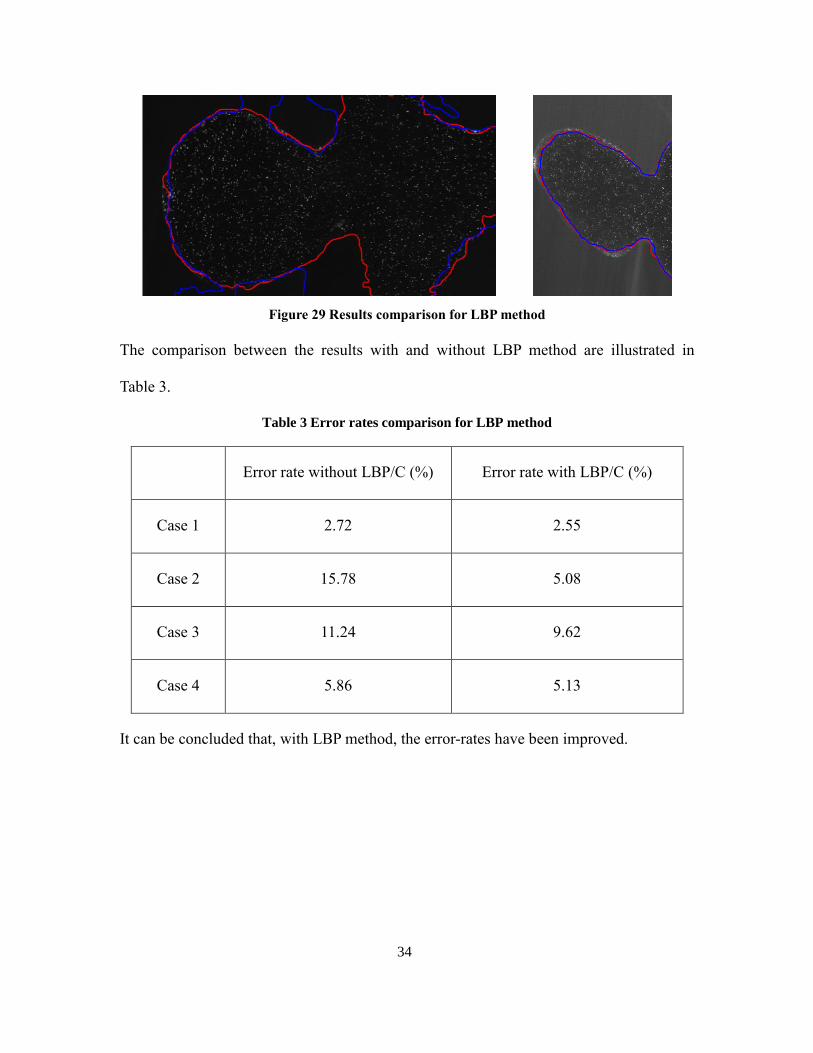
Two examples of the comparison for LBP method is illustrated in Figure 29. For
case 2, Bhattacharyya distance alone is insufficient in segmented the image properly. For
other case, LBP method can effectively improve the segmentation.
34
Figure 29 Results comparison for LBP method
The comparison between the results with and without LBP method are illustrated in
Table 3.
Table 3 Error rates comparison for LBP method
Error rate without LBP/C (%) Error rate with LBP/C (%)
Case 1 2.72 2.55
Case 2 15.78 5.08
Case 3 11.24 9.62
Case 4 5.86 5.13
It can be concluded that, with LBP method, the error-rates have been improved.
35
Chapter 5
DISCUSSION
In this chapter, the analysis of the results is presented and several directions for
future research are proposed. Section 5.1 discusses the results of the algorithm. Section 5.2
illustrates some directions of future work.
5.1 Results Analysis
A PIV image can be segmented into two region, one is the non-particle part and
another is the particle-containing part. Both of these two parts contain a background where
the intensity is almost uniform. For non-particle part, the image consists of a background
and noise from the CCD camera. For the particle part, the image consists of a background
and some particles on it. There are two major factors that impact the final result of the
segmentation. One is the intensity level of the background of both particle and non-particle
part. Another is the density of particles in the particle part. All input images can be
classified into four categories (from best to worst): 1) different backgrounds and high
particle density. 2) different backgrounds and low particle density, 3) uniform backgrounds
and high particle density, 4) uniform backgrounds and particle low density.
The intensity levels of the backgrounds are critical for the results of the
segmentation as he background intensity levels greatly determine the BC. Figure 27 shows
how the backgrounds and the particle density influence the results. The solid red line
illustrates the histogram of the sample region and the dotted line represents the histogram
of a non-particle block in the image that is compared to the sample region. The peak of
these two lines indicate the intensities of the backgrounds in the sample region and the
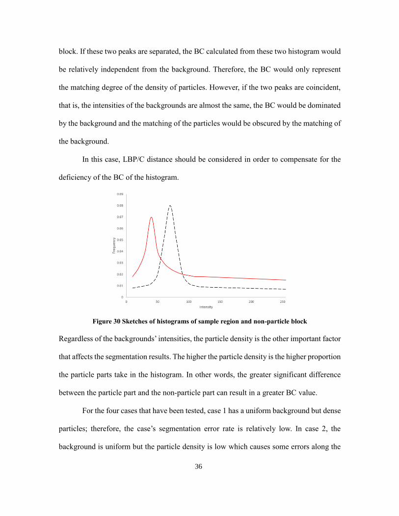
36
block. If these two peaks are separated, the BC calculated from these two histogram would
be relatively independent from the background. Therefore, the BC would only represent
the matching degree of the density of particles. However, if the two peaks are coincident,
that is, the intensities of the backgrounds are almost the same, the BC would be dominated
by the background and the matching of the particles would be obscured by the matching of
the background.
In this case, LBP/C distance should be considered in order to compensate for the
deficiency of the BC of the histogram.
Figure 30 Sketches of histograms of sample region and non-particle block
Regardless of the backgrounds’ intensities, the particle density is the other important factor
that affects the segmentation results. The higher the particle density is the higher proportion
the particle parts take in the histogram. In other words, the greater significant difference
between the particle part and the non-particle part can result in a greater BC value.
For the four cases that have been tested, case 1 has a uniform background but dense
particles; therefore, the case’s segmentation error rate is relatively low. In case 2, the
background is uniform but the particle density is low which causes some errors along the
37
border. Case 3 is the worst case due to its complicated backgrounds and as out-of-focus
regions. Case 4 also has complicated backgrounds and out-of-focus areas.
5.2 Methods Analysis
As introduced in Section 1.2, some other methods are used for image segmentation.
Region splitting and merging is a good method to perform texture segmentation. However
there are problems with this method. This algorithm does not guarantee that each subset is
merged with the best adjacent region. A small variation in the lower level of the merging
stage, like geometrical translation or image noise, causes significant error in the final result.
A pixel-wise classification or boundary smoothing is needed since the regions are
combined by squared regions that are partitioned by a splitting criteria.
Active contour model or other boundary-based methods rely on the properties on
the edges like gradients, but gradients are very discontinuous at the edges in particle images
which causes difficulties to estimate a proper energy function to get rounded boundary
information.
Machine learning techniques are also used in image segmentation [12,13]. For this
method, the accuracy increases with more data. However, for this research, there is
insufficient training data to be used to satisfy the broad sample request of machine learning
techniques.
5.3 Future Work
To make the segmentation more accurate and robust for various applications, there
are several issues left to be further work and implemented.

38
The size of the window used to calculate the histogram and LBP/C can be self-
adapting according to the location.
Once the particle part has been segmented by the combined distance at the first time,
active contour method can be used to refine the boundary.
The thresholding process can be automated by other methods to improve the
algorithm’s automation.
Multiple particle parts can be considered and segmented by the combined distance.
39
Chapter 6
CONCLUSION
This thesis implements an algorithm that can segment a particle image by utilizing
BC and LBP method.
In this thesis, the contributions can be summarized as follows:
The segmentation algorithm is based on the BC and local binary pattern (LBP)
method. This method not only accounts for the intensity but also for the texture feature.
The segmentation results illustrate the improvements via the combined method.
Different PIV images are used to test the segmentation algorithm. The thresholds
are set manually by estimating the proper value for segmentation based on the combined
distance image. The results show the geometry within a PIV image are correctly segmented
by this algorithm.
40
REFERENCES
[1] Gonzalez, R. C. (2009). Digital image processing. Pearson Education India.
[2] Lasheras, J. C. (2007). The biomechanics of arterial aneurysms. Annu. Rev. Fluid
Mech., 39, 293-319.
[3] Adrian, R. J., & Westerweel, J. (2011). Particle image velocimetry (No. 30). Cambridge
University Press.
[4] Nammalwar, P., Ghita, O., & Whelan, P. F. (2010). A generic framework for colour
texture segmentation. Sensor Review, 30(1), 69-79.
[5] Ojala, T., & Pietikäinen, M. (1999). Unsupervised texture segmentation using feature
distributions. Pattern Recognition, 32(3), 477-486.
[6] Kass, M., Witkin, A., & Terzopoulos, D. (1988). Snakes: Active contour models.
International journal of computer vision, 1(4), 321-331.
[7] Michailovich, O., Rathi, Y., & Tannenbaum, A. (2007). Image segmentation using
active contours driven by the Bhattacharyya gradient flow. Image Processing, IEEE
Transactions on, 16(11), 2787-2801.
[8] Boykov, Yuri, and Olga Veksler. "Graph cuts in vision and graphics: Theories and
applications." In Handbook of mathematical models in computer vision, pp. 79-96.
Springer US, 2006.
[9] Bhattachayya, A. (1943). On a measure of divergence between two statistical
population defined by their population distributions. Bulletin Calcutta Mathematical
Society, 35, 99-109.
[10] Ojala, T., Pietikäinen, M., & Harwood, D. (1996). A comparative study of texture
measures with classification based on featured distributions. Pattern recognition, 29(1), 51-
59.
[11] Babiker, M. H., Gonzalez, L. F., Ryan, J., Albuquerque, F., Collins, D., Elvikis, A., &
Frakes, D. H. (2012). Influence of stent configuration on cerebral aneurysm fluid
dynamics. Journal of biomechanics, 45(3), 440-447.
[12] Artan, Y. (2011, May). Interactive image segmentation using machine learning
techniques. In Computer and Robot Vision (CRV), 2011 Canadian Conference on (pp. 264-
269). IEEE.
41
[13] Lee, S. H., Koo, H. I., & Cho, N. I. (2010). Image segmentation algorithms based on
the machine learning of features. Pattern Recognition Letters, 31(14), 2325-2336.
[14] Schmidt, F. R., Toppe, E., & Cremers, D. (2009, June). Efficient planar graph cuts
with applications in computer vision. In Computer Vision and Pattern Recognition, 2009.
CVPR 2009. IEEE Conference on (pp. 351-356). IEEE.
[15] Wu, Z., & Leahy, R. (1993). An optimal graph theoretic approach to data clustering:
Theory and its application to image segmentation. Pattern Analysis and Machine
Intelligence, IEEE Transactions on, 15(11), 1101-1113.
[16] Gdalyahu, Y., Weinshall, D., & Werman, M. (2001). Self-organization in vision:
stochastic clustering for image segmentation, perceptual grouping, and image database
organization. Pattern Analysis and Machine Intelligence, IEEE Transactions on, 23(10),
1053-1074.