Particle Physics Activities for High School Physics Students

Muon Decay in the MINERvA Experiment Margaret Menzies – Harbor City International School, Duluth, MN

Jackie Kitchenhoff ­ Northland High School, Remer, MN Dr. Richard Gran ­ University of Minnesota Duluth, Duluth, MN

Students use actual MINERvA detector event data to find and record decay events from a particle called a muon, understand how atomic and subatomic decay processes work by seeing them happen. They calculate the average lifetime and half­life for the muon and also study

conservation of energy

Conservation Laws of Collisions (Billiard Ball Collisions on the Particle Scale)

Paul Conrow – Rochester City School District, Rochester, NY Carol Hoffman – Hilton Central School District, Hilton, NY

Jeffrey Paradis – Rush­Henrietta Central School District, Henrietta, NY Paul Sedita ­ Canandaigua City Schools, Canandaigua, NY

Dr. Kevin McFarland – University of Rochester, Rochester, NY Students use actual MINERvA detector event data to find and record particle collision events

between a neutrino and neutron (within the nucleus), understand how conservation of momentum and energy on the particle scale. Calculations made will help determine the original momentum

and kinetic energy of the incoming neutrino.

Editing, Technical Work Dr. Nathaniel Tagg– Otterbein University, Westerville, OH

Rev. July 2015

Table of Contents You will find all of the materials listed below (and additional PowerPoint presentations) on the web page: http://neutrino­classroom.org

Particle Physics Activities for High School Physics Students Table of Contents Introduction

Why do you want MINERvA in your curriculum? The essential questions you can explore with this material Technical details on the Arachne program

Suggested Activity Sequence Particle Pre­Assessment for Students Activity: Radioactive Decay of M&M’s Directions for Simple Arachne Activity: Modeling Radioactive Decay with Dice Activity: Finding Muon Decays with MINERvA

Identifying Decay (Michel) Electrons with Arachne Activity: Measuring the Muon Lifetime Activity: Energy of Decay Electrons (Understanding why the electrons in muon decay have this distribution of energy) Quiz: ‘What is MINERvA’? Activity: Build a Model of MINERvA Activity: Conservation of Momentum when Neutrinos Interact Activity: Neutrino Scattering and the Target Nucleus Standard Model Poster Scavenger Hunt Arachne Scavenger Hunt Additional background information Merging Excel Spreadsheets from Student Groups Teacher background Information for Introducing Histograms to Students Glossary of Terms

Introduction

Why do you want MINERvA in your curriculum? Explore cutting edge science in the fascinating world of particle physics.

Students use real particle physics data to explore two standard physics topics 1. Radioactive decay: the random process and lifetime of a particle called a muon. 2. Measuring conservation of momentum and energy when particles collide.

Insight into how practicing scientists creatively solve problems and explore the unseen world of fundamental particles You don't have to be Einstein to get involved with particle physics. Choose as much or as little as you like to add depth to your physics curriculum, or offer parts as an optional activity for students or an after school science club.

The essential questions you can explore with this material 1. What do your students already know about particle physics? How is the

MINERvA project being used to detect particles that are difficult to observe? What are the signatures of decay and momentum events in the detector?

2. What is radioactive decay, and what is characteristic about the decay of the muon particle? How do I see that radioactive decay is a random process?

3. When subatomic particles collide, their identities often change. Is momentum still conserved?

4. How do I visually represent particle physics data, in order to better draw conclusions? Why are histograms used to analyze data?

5. What is the mean lifetime (and half­life) for decay? What is the distribution of random decay times?

6. How can I use conservation of momentum of the final products of a neutrino collision to learn about the neutrino and the neutron that collided? Was the neutron moving inside the nucleus?

7. How do scientists deal with different interpretations of the same data? What else can be observed in MINERvA?

8. How does special relativity govern the relationships between speed, momentum and energy? What is the connection between E=mc2 and the energy spectrum of the electrons from muon decay?

Technical details on the Arachne program Arachne is named after a character from mythology who lost a weaving contest to MINERvA.

The Arachne program was created in order to visualize particles that were recorded by the MINERvA detector. It pulls calibrated data from a server at Fermilab and then draws a few pictures and graphs to summarize what happened in the detector.

Arachne requires a recent version of a web browser, such as Firefox version 4.0, Safari version 4.0, and Chrome version 5.0. Arachne relies on Java and parts of the HTML5 standard to more dynamically render the images and make them interactive. Because it does not yet support the latter, the Internet Explorer browser will not run Arachne. The day before your class, be sure to check that the server is responding. It occasionally goes down.

Suggested Activity Sequence There are a number of interesting things so see in the MINERvA data, but we have chosen two different threads that illustrate and reinforce ideas that are already part of your physics and chemistry curriculum. Muon Decay is an example of radioactive decay. In chemistry or physics class, the concept seems abstract, something that happens unseen inside lumps of material like uranium or aging trees. These activities let you observe real decays and measure their decay time one­by­one, in the comfort of your own classroom. In the MINERvA detector particles with charge produce visible tracks that can be followed, which is what this activity is all about, using real­event data showing muon decay to Michel electrons. They are named for Louis Michel (1923­1999), the French physicist who provided the first documentation of the decay sequence of muons to an electron and two neutrinos: A development not so different from Marie Curie's pioneering initial work on radioactive decay. MINERvA is capable of detecting an array of events. We will be focused on muon decay events in these activities, but students are likely to observe other events if they do any exploring of data on their own. (Arachne Scavenger Hunt) Further background on the types of events detected in MINERvA is outlined in a PowerPoint presentation on Types of Events.

Billiard Ball Collisions involving conservation of momentum and energy, is a familiar introductory physics topic. The same conservation principles and visualization applies to particle interactions, too. The simplest examples even look like the collision of two billiard balls, but also reveal something of the inner workings of the atomic nucleus. Below, we suggest a sequence of activities for each topic. Depending on your class, schedule, or other considerations, you can shorten the activities, or in some cases assign pieces as homework instead of doing them in class.

Muon Decay Activities Introductory Activities ­ (I) Data Analysis­ (DA) Enrichment Activities ­ (E) Prior Knowledge Activities: (I) Particle Pre­Assessment for Students (I) Particle Adventure1 (I) Standard Model Poster scavenger hunt (DA) Histogram Activities3 Classroom Activities: (I) Activity: Modeling radioactive decay with dice (60 minutes) (I) Activity: Radioactive Decay of M&M’s (I) What is MINERvA? – PowerPoint (20 minutes) (I) Directions for Simple Arachne (Arachne basics for muon decay) ­ Tutorial (20 minutes) (I) Activity: finding muon decays with MINERvA­ teacher guided (30 minutes) (I) History of the Neutrino “Norton Nabs a Nu” – PowerPoint (30 minutes) (E) Types of Events – PowerPoint (30 minutes) (DA) Activity: Measuring the muon lifetime (90 minutes), data analysis, calculations and graphing data (180 minutes), Optional/Extension Activities: (E) Arachne Scavenger Hunt (DA) Neutrino Birth and Death PowerPoint (I) Activity: Build a model of MINERvA (E) Activity: Energy of Decay electrons (Understanding why the electrons in muon decay have this distribution of energy) (I) Particle Events in 60 seconds (I) See what the MINERvA detector is doing right now (E) Neutrinos in 60 seconds (E) Kevin McFarland’s neutrino talk for students

Billiard Ball Collisions (Conservation Laws) on the Particle Scale Introductory Activities ­ (I) Data Analysis­ (DA) Enrichment Activities ­ (E) Prior Knowledge Activities: (I) Particle Pre­Assessment for Students (I) Particle Adventure1 (I) Standard Model Poster scavenger hunt (DA) Histogram Activities2 Classroom Activities: (I) History of particle physics and MINERvA – PowerPoint (30 minutes) (I) What is MINERvA? – PowerPoint (30 minutes) (I) Directions to Simple Arachne – Tutorial (30 minutes) (I) Bug and Truck Collision – PowerPoint (30 minutes) (I) Activity: Conservation of momentum when neutrinos interact– teacher guided (60 minutes) (I) Ten collision sampler (30 minutes) (I) MINERvA Momentum Model – PowerPoint (30 minutes) (I) History of the Neutrino “Norton Nabs a Nu” – PowerPoint (30 minutes) (DA) Activity: Neutrino scattering and the target nucleus (60 minutes), Continue data analysis Optional/Extension Activities: (E) Arachne Scavenger Hunt (DA) Neutrino Birth and Death PowerPoint (I) Activity: Build a model of MINERvA (I) See what the MINERvA detector is doing right now (E) Neutrinos in 60 seconds (E) Kevin McFarland’s neutrino talk for students 1 ­ Particle Adventure is an excellent online resource that provides a fairly quick introduction to particle physics and fundamental particles. It was produced and is maintained by the Particle Group of the Lawrence Berkeley National Laboratory. Here is the website: http://www.particleadventure.org/index.html. Once at the website, choose “The Standard Model” option. This is divided into four major parts. For a good unit introduction we suggest using “What is fundamental?”, and “What is the world made of?” “What holds it together?” follows these first two and should be considered optional as it provides background on fundamental forces and their interactions which is not critical to this unit's focus. “Particle decays and annihilations” follows this section and should be used with students to provide some overview of decay 2 ­ Histogram activities are provided if you think your students could use further background in the purposes, construction and appropriate uses of histograms for scientific data.

Particle Pre­Assessment for Students Goal A quick assessment for teachers to use to gauge the content that students already have in the topic of modern physics. Notes for the Teacher Each student enters physics with a different set of knowledge. This questionnaire is meant for the students to take so that the teacher can determine what Prior Knowledge Activities might be appropriate so that the students feel more comfortable heading into the unit. Student Instructions and Worksheet

Particle Physics Pre­Assessment Directions: Answer each of the following questions with honesty and thorough thought. The answers that you give are going to help your teacher structure your particle physics unit.

1. How comfortable are you with the main principles and concepts of particle physics?

Very Comfortable Comfortable Barely

Comfortable Not Very

Comfortable 2. What, if any, value do you see in learning particle physics in high school? Explain why. 3. Where would you get information about particle physics? _______ Wikipedia

_______ other

websites

_______textbooks

_______ textbook extras

________ other students

________ other

4. What scenarios would you use to illustrate momentum conservation in physics class?

5. What is the connection between momentum and particle physics?

6. What are the fundamental particles of matter? 7. What do you know about quarks and/or neutrinos? 8. What is antimatter? 9. In addition to electric charge, what is conserved in particle reactions? 10. What is E = mc2 all about?

11. What does LHC stand for & why has it been in the news in the past year?

12. What are the basic principles of physics that explain the operation of particle accelerators

(feel free to include diagrams)?

13. What is a histogram (include a chart with axis titles)? 14. What are histograms used for?

15. Why are histograms important to particle physics analysis?

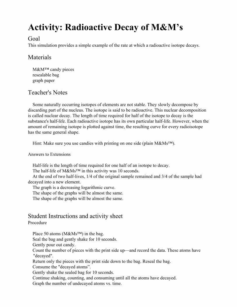
Activity: Radioactive Decay of M&M’s Goal This simulation provides a simple example of the rate at which a radioactive isotope decays. Materials M&M™ candy pieces resealable bag graph paper Teacher's Notes Some naturally occurring isotopes of elements are not stable. They slowly decompose by discarding part of the nucleus. The isotope is said to be radioactive. This nuclear decomposition is called nuclear decay. The length of time required for half of the isotope to decay is the substance's half­life. Each radioactive isotope has its own particular half­life. However, when the amount of remaining isotope is plotted against time, the resulting curve for every radioisotope has the same general shape. Hint: Make sure you use candies with printing on one side (plain M&Ms™). Answers to Extensions Half­life is the length of time required for one half of an isotope to decay. The half­life of M&Ms™ in this activity was 10 seconds. At the end of two half­lives, 1/4 of the original sample remained and 3/4 of the sample had decayed into a new element. The graph is a decreasing logarithmic curve. The shape of the graphs will be almost the same. The shape of the graphs will be almost the same. Student Instructions and activity sheet Procedure Place 50 atoms (M&Ms™) in the bag. Seal the bag and gently shake for 10 seconds. Gently pour out candy. Count the number of pieces with the print side up—and record the data. These atoms have "decayed".

Return only the pieces with the print side down to the bag. Reseal the bag. Consume the "decayed atoms”. Gently shake the sealed bag for 10 seconds. Continue shaking, counting, and consuming until all the atoms have decayed. Graph the number of undecayed atoms vs. time.

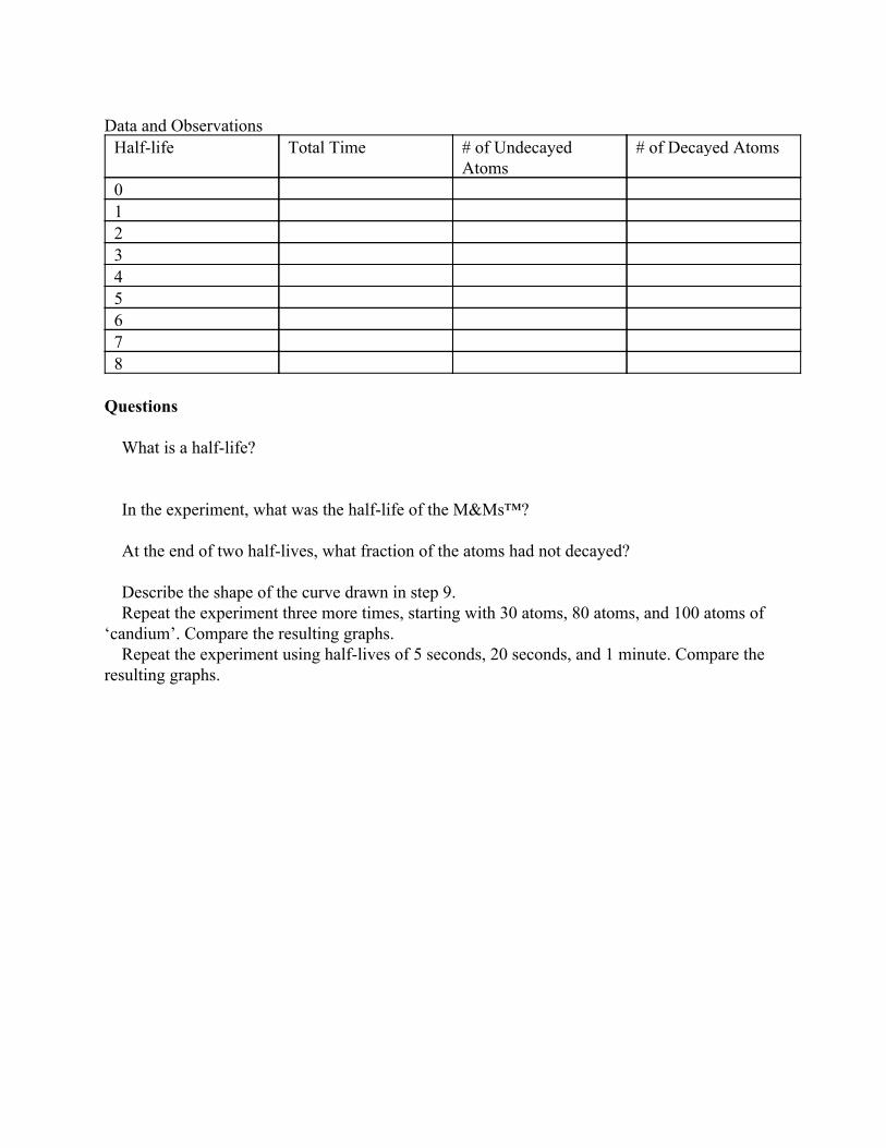
Data and Observations Half­life Total Time # of Undecayed

Atoms # of Decayed Atoms

0 1 2 3 4 5 6 7 8 Questions What is a half­life? In the experiment, what was the half­life of the M&Ms™? At the end of two half­lives, what fraction of the atoms had not decayed? Describe the shape of the curve drawn in step 9. Repeat the experiment three more times, starting with 30 atoms, 80 atoms, and 100 atoms of ‘candium’. Compare the resulting graphs. Repeat the experiment using half­lives of 5 seconds, 20 seconds, and 1 minute. Compare the resulting graphs.

Directions for Simple Arachne (Arachne basics for muon decay) Goal: The information below should be reviewed by both the teacher and the students so that everyone has a basic knowledge of how the Arachne site works and relays data

http://minerva05.fnal.gov/Arachne/simple.html

DATA:

(example) MN 1020/10 v7r5p1 – represents the run and Sub­Run number of the event

Entry – This is 16000 ns of time in which a ‘snapshot picture of the event was captured

Prev/Next Gate – this changes the event viewed through the detector during a different 16000 ns of time and corresponds to the Entry #

Prev/Next Slice – this gives you a specific time of the event within the given 16000 ns gate [Analogy: the Run is like a roll of film…the Entry (Gate) is each individual picture on the film… the Slice contains the details within each picture]

TIME HISTOGRAM:

Gives you the indication of time (in ns) where informative events may have occurred. A grey highlighted cursor moves across the histogram as you change Slices.

The y­axis is measured Energy in MeV or in Photoelectrons (PE)

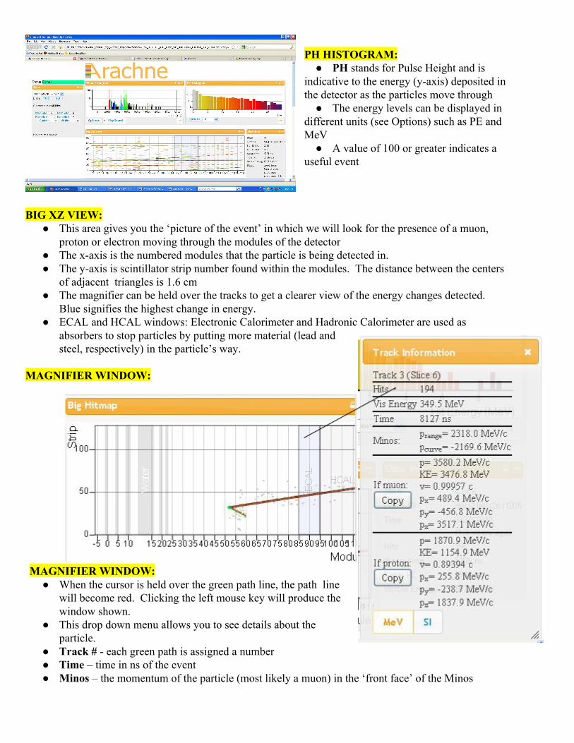
PH HISTOGRAM:

PH stands for Pulse Height and is indicative to the energy (y­axis) deposited in the detector as the particles move through The energy levels can be displayed in

different units (see Options) such as PE and MeV A value of 100 or greater indicates a

useful event

BIG XZ VIEW:

This area gives you the ‘picture of the event’ in which we will look for the presence of a muon, proton or electron moving through the modules of the detector

The x­axis is the numbered modules that the particle is being detected in. The y­axis is scintillator strip number found within the modules. The distance between the centers

of adjacent triangles is 1.6 cm The magnifier can be held over the tracks to get a clearer view of the energy changes detected.

Blue signifies the highest change in energy. ECAL and HCAL windows: Electronic Calorimeter and Hadronic Calorimeter are used as

absorbers to stop particles by putting more material (lead and steel, respectively) in the particle’s way.

MAGNIFIER WINDOW:

MAGNIFIER WINDOW: When the cursor is held over the green path line, the path line

will become red. Clicking the left mouse key will produce the window shown.

This drop down menu allows you to see details about the particle.

Track # ­ each green path is assigned a number Time – time in ns of the event Minos – the momentum of the particle (most likely a muon) in the ‘front face’ of the Minos

detector at Fermi lab If Muon /If Proton – momentum and KE data of the proton and muon are used to determine the

momentum and KE of the original neutrino and neutron prior to the collision. The proton’s path will be shorter, with more energy deposited in a short distance, and the muon’s path will reach beyond the detector, since it loses little energy as it travels. (See 3D display). This information is helpful when determining if the track is that of a proton or muon so that the correct data is recorded. By clicking on the Copy button, the needed information will be copied into an excel document for analysis

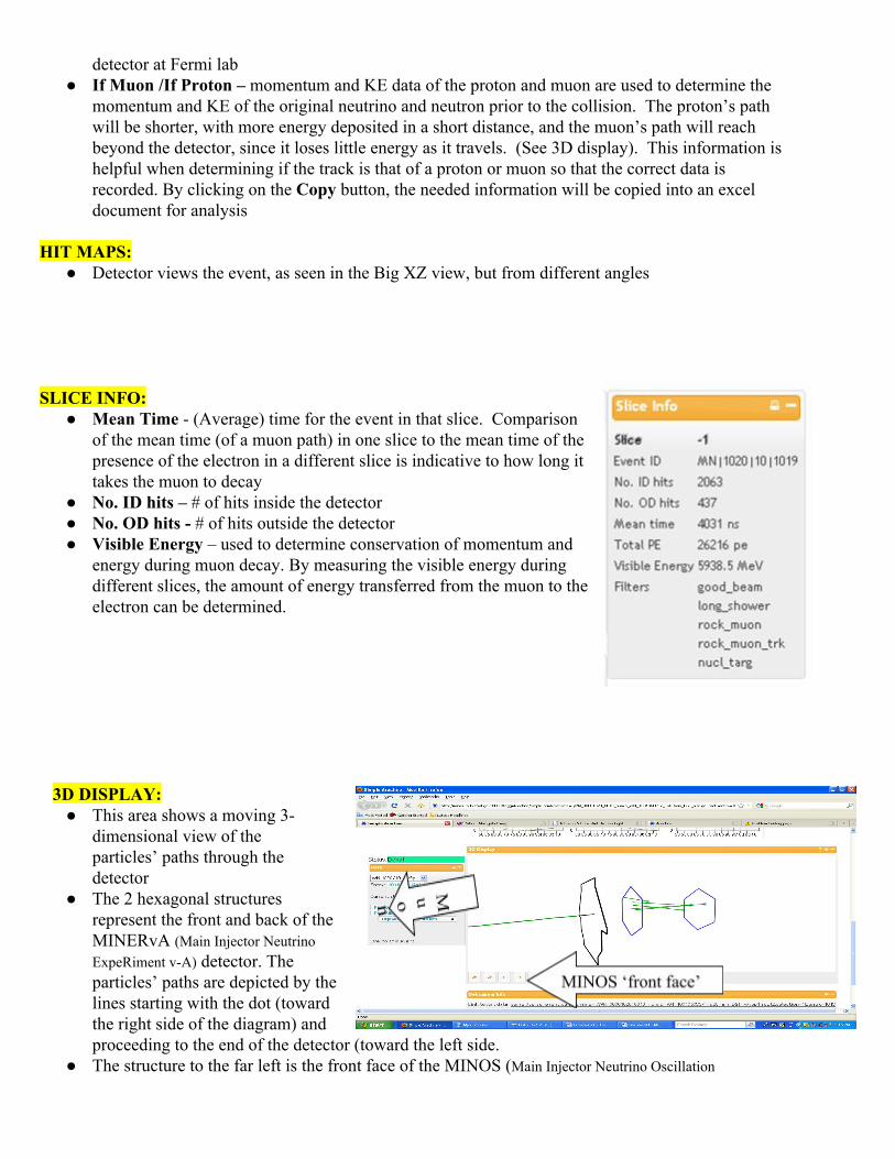
HIT MAPS: Detector views the event, as seen in the Big XZ view, but from different angles

SLICE INFO: Mean Time ­ (Average) time for the event in that slice. Comparison

of the mean time (of a muon path) in one slice to the mean time of the presence of the electron in a different slice is indicative to how long it takes the muon to decay

No. ID hits – # of hits inside the detector No. OD hits ­ # of hits outside the detector Visible Energy – used to determine conservation of momentum and

energy during muon decay. By measuring the visible energy during different slices, the amount of energy transferred from the muon to the electron can be determined.

3D DISPLAY: This area shows a moving 3­

dimensional view of the particles’ paths through the detector The 2 hexagonal structures

represent the front and back of the MINERvA (Main Injector Neutrino ExpeRiment v­A) detector. The particles’ paths are depicted by the lines starting with the dot (toward the right side of the diagram) and proceeding to the end of the detector (toward the left side.

The structure to the far left is the front face of the MINOS (Main Injector Neutrino Oscillation

Search) detector. The MINOS detector is also involved with neutrino detection and is part of an experiment that spans from Fermi lab to Tower Soudan Underground Physics Laboratory in Soudan, Minnesota

If a particle extends beyond the end of the MINERvA detectors and enters in MINOS, than it is most likely a muon particle.

Activity: Modeling Radioactive Decay with Dice This is the first activity in learning about radioactive decay

Goals

1. Start with a physical, tactile simulation of radioactive decay. 2. See the exponential and random nature of a decay process directly. 3. Play dice with the Universe.

Radioactive decay, as it is often taught, is abstract. We talk about piles of radioactive material, a “decaying exponential” mathematical function, and how it is dangerous, but these things are happening at an atomic level we can't actually see or experience with our hands or eyes directly. The two variations here let us do that, making clear both the intrinsically random, but at the same time the intrinsically exponential nature of the process. Then in muon decay activity two, with data from MINERvA, we will take an actual decay process which is also usually unseen, and make it visible too.

Prior Knowledge: Examples of radioactive decay from the news or elsewhere, such as carbon­14, the M&Ms™ lab, medical tracer isotopes, or the storage of nuclear waste.

Materials: Dice Paper to record the data, graph paper to make a histogram Calculator

Notes for the teacher What is radioactive decay, and what other things in nature share the same characteristics? The process of radioactive decay, of atomic isotopes or fundamental particles, is intrinsic to the universe and to particle physics. The mathematically characteristic exponential decay (and the related exponential growth) is found in lots of places in nature; anywhere the rate of change of something is proportional to the amount of that something. Radioactive isotopes, bacteria populations, investments in a bank account. The other characteristic of radioactive decay is its inherent randomness, which is pretty astounding by itself, and is a core feature of quantum mechanical systems. The random nature also leads to some interesting issues in observing and

measuring the decay, problems shared with other inherently random things such as political polling and the ubiquitous ±3% error and separately with rolling dice. These activities use the dice process to give you a tactile, physical experience with what is really happening in these other processes that are nanoscopic or abstract. There are two related pieces here. Rolling one hundred dice several times, and rolling a single die multiple times, then repeating that a hundred times. Here, we've assumed you are able to do both, possibly saving the second one as an out­of­lab homework activity. It is reasonable that, due to time or material constraints, you choose to do only the second one or only the first. If you picked this up with the MINERvA muon decay activities, the second one is the most like what the students will experience looking at muon decay. The two ways are first summarized here, together. The student instructions break them into two separate, with specific instructions and questions for the group doing the activities. First way: roll one hundred dice (multiple times) to represent a sample of a hundred radioactive isotopes decaying over time. This does a good job of illustrating the idea of "half­life" and the exponential decrease in the activity of a radioactive sample over time. The question you are asking is “how many remain after some time”. Such samples might be medical isotopes, waste from your local nuclear reactor, or the uranium and thorium atoms that remain on earth long after they were formed ten billion years ago in supernovae. Second way: roll a single die (multiple times) to represent how long a single muon lives, then do it again for the next muon, and the next, one hundred times. This is a good way to illustrate the range of lifetimes you will observe if you have a sample of unstable particles such as muons. The question you are quantifying is “how long (what range of times) does each particle live”. Such samples are common in particle and nuclear physics. In fact, these two illustrations are just two ways of looking at the same phenomena. After doing one or both activities, it should be clear that you are observing a random process, observing many at once, or one at a time doesn't matter, and they both lead to the exponential decay that is characteristic of the random process. This will also help overcome the problem that you can't “see” radioactive isotopes or muons; it makes these real but hidden details plain. As a bonus, you will also observe how the randomness also means you will get somewhat different results when you repeat a measurement with otherwise identical initial conditions, such as you might have noticed applies to political polling, and maybe baseball, among other everyday phenomena. Doing the second variation only: If you are not able to obtain enough dice, you can do the second activity only. And anyway, the second variation better matches the muon decay activities involving the MINERvA data. When you prepare the instructions for students, trim out the references to the first variation. Doing the second variation as homework: If you think it is likely that your students have at least one board game at home with dice, you can assign the second activity (which takes more time) as homework, and have each student bring their results in for discussion and be ready for the muon data. Using spreadsheets or other software: This exercise is designed to be done with paper and pencil and calculator, but for students who are prepared, interested, and want to, you can use computer software such as Excel or more advanced software like Matlab, to explore things more quantitatively. We recommend you press on quicker to get to the muon decays in the MINERvA data, but you might know just the student who wants something more advanced.

Instructions for students

What is radioactive decay, and what other things in nature share the same characteristics? The process of radioactive decay, of atomic isotopes or fundamental particles, is intrinsic to the universe and to particle physics. The mathematically characteristic exponential decay (and the related exponential growth) is found in lots of places in nature; anywhere the rate of change of something is proportional to the amount of that something: radioactive isotopes, bacteria populations, investments in a bank account. The other characteristic of radioactive decay is its inherent randomness, which is pretty astounding by itself, and is a core feature of quantum mechanical systems. The random nature also leads to some interesting issues in observing and measuring the decay, problems shared with other inherently random things such as political polling and its ubiquitous ±3% error and separately with rolling dice. These activities use the dice process to give you a tactile, physical experience with what is really happening in these other processes that are nanoscopic or abstract.

First way: one hundred at once. You need: a large supply of dice (about one hundred), a cup or bucket large enough for them, a sheet of paper to record data, and some graph paper for graphing your results. Imagine: you have a supply of some radioactive isotope that has a 1/6 chance of decaying in the next minute. How much of that isotope remains after six minutes? How about after 20 minutes? How much time does it take for approximately half the sample to decay? Put all the dice in your cup or jar and roll them on the table. Separate all the dice that turned up “1”, these are the particles that decayed. Count and record those that decayed and those that remain, measured after “one minute” passed. Separate the decayed “ones” into a pile that you can see later, while you roll the non­ones again. Consider: is the pile of decayed dice about as many as you expect? Was it exactly as many as you expected? Put the others (the ones showing 2­6) back into the cup. Repeat all these steps and record a measurement of what decayed during and what remains after two minutes. Separate this next batch of dice that turned up “1” into its own pile next to the first – you will save the progression of decays so you can see the process visually, in addition to the numbers you have recorded. Repeat again for the third minute. Repeat again and again until they are all decayed. You now have a sequence of piles you can see (and numbers recorded that you can graph) that represent how many decays happened during each minute. Describe you can see both these seemingly contradictory properties: a) the number of decays is proportional to the number available to decay and b) the number that decayed is random. Let’s represent the situation with a couple graphs. Graph the number that decayed in each minute, using a histogram or bar chart. Separately, graph the number that remain undecayed in the sample, using a histogram or bar chart.

Estimate from your graph, by counting, how much time it takes for approximately half the sample to decay. Draw a mark or an arrow on the horizontal axis of each graph indicating where this time is. Look up the exponential decay function; if you have a graphing calculator or similar program, plot it with a constant of (0.16666666 = 1/6), in other words, plot with its negative sign: e­(1/6)x . If you have a regular calculator, compute ten or so values and make another graph of it on your paper. Does that function describe the data you graphed? If you have access to the right software, you might even be able to plot your data and ask the software to fit an exponential, but sketching this one by hand would be good enough. Does the inherent randomness of this process make it difficult to see the exponential nature, and if so, can you think of a change in your procedure How do you feel about the idea that there was likely a die that remained and didn't decay for fifteen to twenty rolls? Is it possible that one could remain for a hundred or more rolls?

Second way: simulating one hundred separate muons You need: one (or a few) dice, a bit of time, a few pieces of paper for recording your data, and a couple more for graphing. Imagine: you are creating, and then observing an unstable particle like a muon or a neutron, and can measure how long each one of them lives, one by one. Each one has a 1/6 chance of decaying in the next one nanosecond, you will count the number of nanoseconds until each one decays. Do you expect short lifetimes to be more common, or long lifetimes, or something in the middle? What is the longest you expect to see a particle live? Can you guess what the average (mean) lifetime will be, when you are done and have analyzed all the decays? Take your die and count the number of rolls until you roll a “1”, and record it on your piece of paper. Repeat about 100 times, each time recording the number of rolls until you roll the number “1”. You have some quality time during this activity to consider the questions mentioned in the “imagine” paragraph above, and what you learned from activity one. (You could divide the effort among three or four people and get it done in 1/3 or 1/4 the amount of time, if you are in a hurry.) Let’s graph the results. Look at the data, and count the number of times where the muon lasted up to one nanosecond. Record that on a graph in the 0­1 interval. Count the number of times it took two rolls, and record that in the 1­2 interval. You are making a histogram of the decay time. Continue until you have filled all the intervals; toward the end many of them will be filled with zeros, with occasional intervals where a few long­lived particles fall. Now compute the average life, in nanoseconds. Clearly you can average all 100 numbers you recorded by adding them and dividing by 100. You might see that you can do this more quickly from your graph than you can from the sheet with 100 numbers on it, but either way works. Draw a mark on the horizontal axis of your graph to represent the average lifetime. Look up the exponential decay function; if you have a graphing calculator or similar program, plot it with a constant of (0.16666666 = 1/6), in other words, plot with the negative sign: e­(1/6)x .

Does that function describe the data you graphed? Does the inherent randomness of this process make it difficult to see the exponential nature, and where is it the most difficult? Why? How do you feel about the idea that there was likely a muon that remained and didn't decay for fifteen to twenty rolls? Is it possible that one could remain for a hundred or more rolls? Now what are your answers to these questions: do you expect short lifetimes to be more common, or long lifetimes, or something in the middle? What is the longest you expect to see a particle live? If you have done both exercises, your one graph from the second exercise is most like which graph from the first exercise? And it should look approximately like the other graph from the first exercise, but 6 times smaller. In these cases, they should look similar enough that you can recognize the similarity, but they certainly won't be identical. How would you explain why they should look so similar but not identical? What would happen if you repeated one or the other exercise again, would the results be identical? For both exercises, you had one die that lasted the longest, but might you ever expect to see a particle last ten­times that long? What would happen if you had the luxury of doing 1,000 trials, or 1,000,000 trials, or an Avogadro’s number (6.02 x 1023) number of trials?

The function that best describes these graphs is a decaying exponential Ne­t/τ, (sometimes also written Ne­λt ) where our situation is such that t is time, N is either the initial number of particles that might decay, or the initial activity which is 1/6 of the number of particles, and τ (tau) is the mean lifetime which is 6 seconds or nanoseconds depending on which activity you are doing or λ which is the probability that a particle will decay in the next bit of time. This function occurs a lot for interesting random and non­random situations, but random processes often give rise to behavior that can be described mathematically like this. Notice, in the second activity you directly measured the value of this parameter τ tau = mean lifetime. If you recognized how the second activity is the same as the first, then you have again measured it. Go back to your first data set and calculate the mean lifetime there. Is it the same? Should it be? What is the accuracy of your measurement and the role of random fluctuations in your measurement? If you had a need to make a more accurate measurement, how would you do it?

Advanced questions: You might notice that the spot where you marked “half­life” in the first activity is not at all in the same location as the spot you marked “mean­life” in the second activity. These are different. Think carefully about how you knew where to mark those spots and try to describe the subtle difference between them. Political polling has been mentioned as another random process that we suppose you have encountered. Though it doesn't obviously give rise to an exponential distribution, but it clearly does give rise to fluctuations between repeated measurements of apparently the same thing, such

as the public's support one or the other political candidate. If you don't expect two polling firms to get the same answer if they poll on the same night, how can you still draw conclusions from their results? I teased that the same issues involving random processes might also apply to the game baseball. Think on that. If you are comfortable enough with your calculus, you can derive the connection between the probability to decay and the exponential function. An internet search or textbook will get you started. If you are comfortable enough with programming, and can find a pseudo­random number generator to use, you can explore further and faster than you can with dice. Using the same 1/6 probability, code the procedure into a program. Use a programming platform like C++, Java, Matlab, Mathematica, or possibly even a spreadsheet. When it's ready, play with the mean lifetime and compare the exponential to high statistics histograms. Then play with changing the time step or probability.

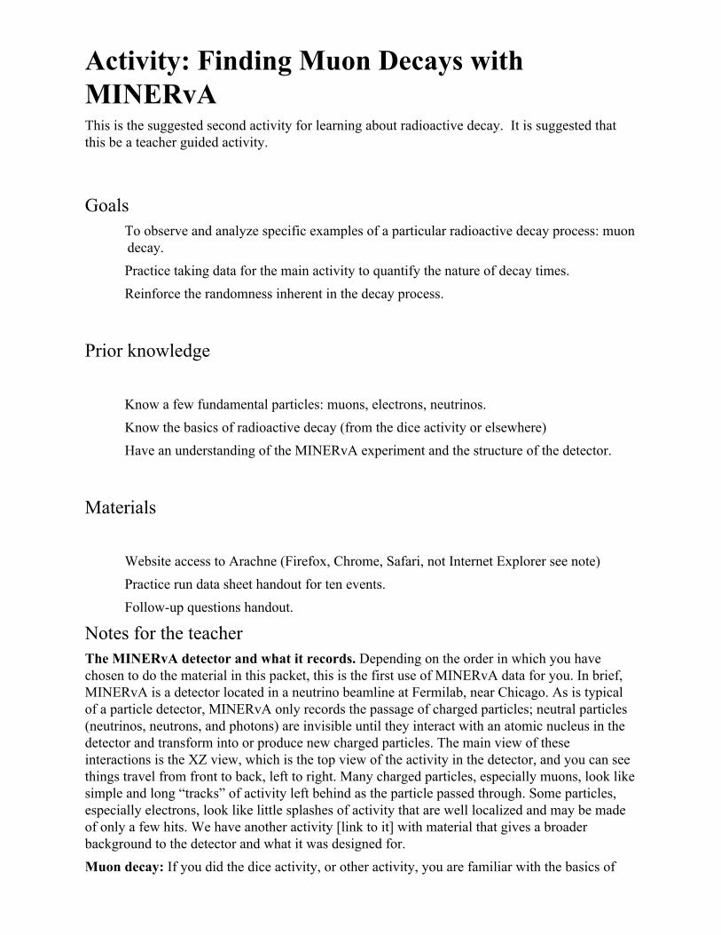
Activity: Finding Muon Decays with MINERvA This is the suggested second activity for learning about radioactive decay. It is suggested that this be a teacher guided activity.

Goals

To observe and analyze specific examples of a particular radioactive decay process: muon decay.

Practice taking data for the main activity to quantify the nature of decay times. Reinforce the randomness inherent in the decay process.

Prior knowledge

Know a few fundamental particles: muons, electrons, neutrinos. Know the basics of radioactive decay (from the dice activity or elsewhere) Have an understanding of the MINERvA experiment and the structure of the detector.

Materials

Website access to Arachne (Firefox, Chrome, Safari, not Internet Explorer see note) Practice run data sheet handout for ten events. Follow­up questions handout.

Notes for the teacher The MINERvA detector and what it records. Depending on the order in which you have chosen to do the material in this packet, this is the first use of MINERvA data for you. In brief, MINERvA is a detector located in a neutrino beamline at Fermilab, near Chicago. As is typical of a particle detector, MINERvA only records the passage of charged particles; neutral particles (neutrinos, neutrons, and photons) are invisible until they interact with an atomic nucleus in the detector and transform into or produce new charged particles. The main view of these interactions is the XZ view, which is the top view of the activity in the detector, and you can see things travel from front to back, left to right. Many charged particles, especially muons, look like simple and long “tracks” of activity left behind as the particle passed through. Some particles, especially electrons, look like little splashes of activity that are well localized and may be made of only a few hits. We have another activity [link to it] with material that gives a broader background to the detector and what it was designed for. Muon decay: If you did the dice activity, or other activity, you are familiar with the basics of

radioactive decay. A particle or nucleus spontaneously (and randomly) changes into one or more new particles (or a new nucleus and some particles). The resulting state is energetically favorable, so there is always additional energy available to become kinetic energy. Specifically, the muon decays similar to the classic “beta decay” (similar to carbon­14 and also like neutron decay) giving an electron and two neutrinos as products. If you are familiar with the standard model of particles, muons are a heavy cousin to the electron; the technical term for this family of particles is leptons. So the muon decays into its less massive lepton cousin. The neutrinos are neutral, so they are usually unseen as they escape the point of the decay, so the signature is a muon stopping in the detector then the electron from the decay appearing. We can write this reaction in a form similar to how we right chemical reactions

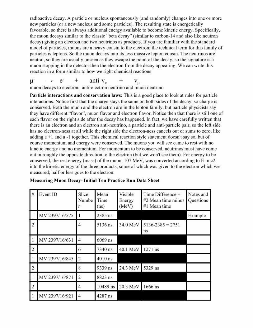
μ­ → e­ + anti­ve + vμ muon decays to electron, anti­electron neutrino and muon neutrino Particle interactions and conservation laws: This is a good place to look at rules for particle interactions. Notice first that the charge stays the same on both sides of the decay, so charge is conserved. Both the muon and the electron are in the lepton family, but particle physicists say they have different “flavor”, muon flavor and electron flavor. Notice then that there is still one of each flavor on the right side after the decay has happened. In fact, we have carefully written that there is an electron and an electron anti­neutrino, a particle and anti­particle pair, so the left side has no electron­ness at all while the right side the electron­ness cancels out or sums to zero, like adding a +1 and a ­1 together. This chemical reaction style statement doesn't say so, but of course momentum and energy were conserved. The muons you will see came to rest with no kinetic energy and no momentum. For momentum to be conserved, neutrinos must have come out in roughly the opposite direction to the electron (but we won't see them). For energy to be conserved, the rest energy (mass) of the muon, 107 MeV, was converted according to E=mc2 into the kinetic energy of the three products, some of which was given to the electron which we measured; half or less goes to the electron. Measuring Muon Decay­ Initial Ten Practice Run Data Sheet # Event ID Slice

Number

Mean Time (ns)

Visible Energy (MeV)

Time Difference = #2 Mean time minus #1 Mean time

Notes and Questions

1 MV 2397/16/575 1 2385 ns Example

2 4 5136 ns 34.0 MeV 5136­2385 = 2751 ns

1 MV 2397/16/631 4 6069 ns

2 6 7340 ns 40.1 MeV 1271 ns

1 MV 2397/16/845 2 4010 ns

2 8 9339 ns 24.3 MeV 5329 ns

1 MV 2397/16/871 2 8823 ns

2 4 10489 ns 20.3 MeV 1666 ns

1 MV 2397/16/921 4 4287 ns

2 7 11164 ns 30.4 MeV 6877 ns

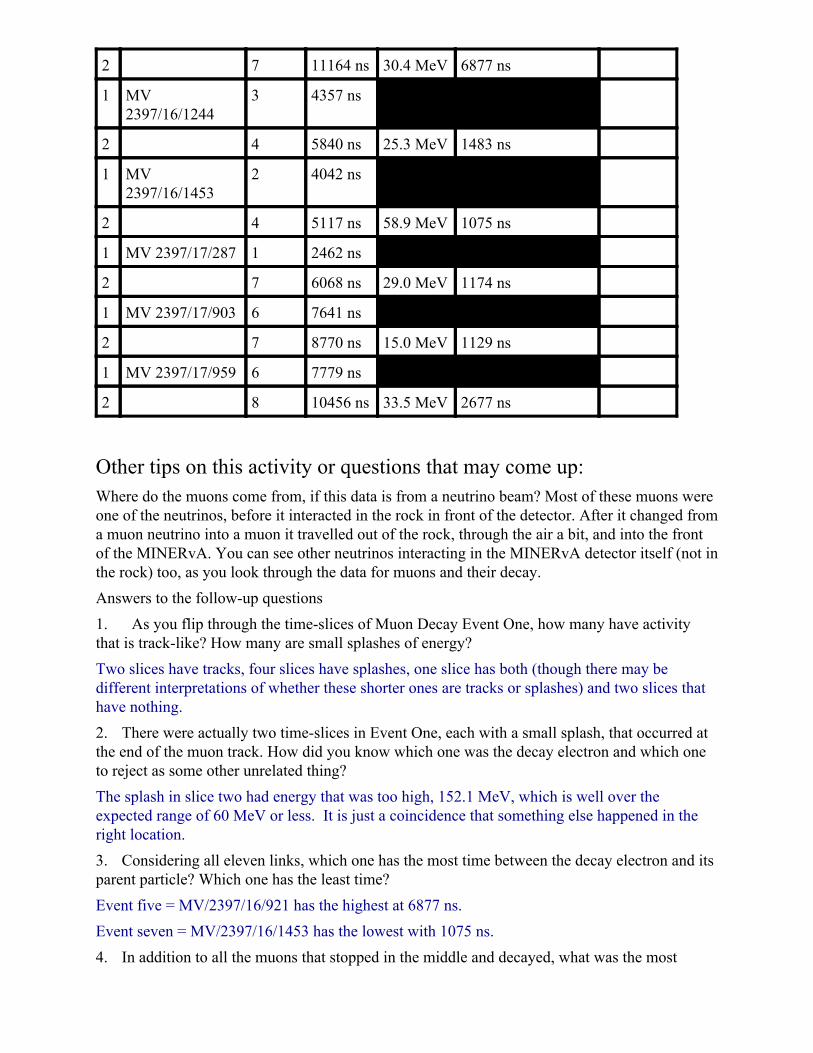
1 MV 2397/16/1244

3 4357 ns

2 4 5840 ns 25.3 MeV 1483 ns

1 MV 2397/16/1453

2 4042 ns

2 4 5117 ns 58.9 MeV 1075 ns

1 MV 2397/17/287 1 2462 ns

2 7 6068 ns 29.0 MeV 1174 ns

1 MV 2397/17/903 6 7641 ns

2 7 8770 ns 15.0 MeV 1129 ns

1 MV 2397/17/959 6 7779 ns

2 8 10456 ns 33.5 MeV 2677 ns

Other tips on this activity or questions that may come up: Where do the muons come from, if this data is from a neutrino beam? Most of these muons were one of the neutrinos, before it interacted in the rock in front of the detector. After it changed from a muon neutrino into a muon it travelled out of the rock, through the air a bit, and into the front of the MINERvA. You can see other neutrinos interacting in the MINERvA detector itself (not in the rock) too, as you look through the data for muons and their decay. Answers to the follow­up questions 1. As you flip through the time­slices of Muon Decay Event One, how many have activity that is track­like? How many are small splashes of energy? Two slices have tracks, four slices have splashes, one slice has both (though there may be different interpretations of whether these shorter ones are tracks or splashes) and two slices that have nothing. 2. There were actually two time­slices in Event One, each with a small splash, that occurred at the end of the muon track. How did you know which one was the decay electron and which one to reject as some other unrelated thing? The splash in slice two had energy that was too high, 152.1 MeV, which is well over the expected range of 60 MeV or less. It is just a coincidence that something else happened in the right location. 3. Considering all eleven links, which one has the most time between the decay electron and its parent particle? Which one has the least time? Event five = MV/2397/16/921 has the highest at 6877 ns. Event seven = MV/2397/16/1453 has the lowest with 1075 ns. 4. In addition to all the muons that stopped in the middle and decayed, what was the most

interesting other thing you saw? A variety of answers are possible, though there is a neutrino interaction in the same link as seven in MV/2397/16/1453 that we think stands out as interesting. 5. The muon you find is always traveling left to right, then stopping somewhere in the middle. How about the electrons? Since the muon is at rest when the decay happens, the electron can go in any direction it chooses (it chooses randomly), so it may or may not move in the same direction as the muon travelled. In these ten decays you see all the variations. In contrast, if the muon was moving (its not), then to conserve momentum, the decay electron would probably be moving in roughly the same direction. 6. Describe in your own words, what is radioactive decay, and specifically how does a muon decay. Radioactive decay happens when an unstable particle or a whole atom tries to settle into a more stable state. It happens randomly, with both long and short times. (In the next activity, we will measure the characteristic decay time, despite the randomness.) A muon specifically decays to form a Michel electron and two neutrinos, of which only the electron is visible in the MINERvA data. For sure I notice that charge is conserved. There is a negative charged thing on both sides. [If you have covered all the conservation laws, then the answer might continue as follows. Rules of particle decay require charge to be conserved (­1 on both sides). Lepton family/flavor must be conserved: there is muon­type flavor on both sides, there is no electron flavor in the initial state, but there is both electron and anti­electron (neutrino) flavor in the final state, which is like adding +1 and ­1 for a net zero. ]

Identifying Decay (Michel) Electrons with Arachne

To access the Arachne program, start by clicking on the following web link.

Muon Decay Event One: http://minerva05.fnal.gov/Arachne/simple.html?filename=/minerva/data/users/minervapro/outreach/muondecayDST/v10r6_2397/97/MV_00002397_0016_numip_v05_1007120650_RecoData_DST_v10r6.root&entry=306&slice=­1&phCutLow=0.5 The display shows all the activity in the MINERvA detector for a single, short pulse of neutrinos. Of the few buttons on the page, you are most concerned with the “Prev slice” and “Next slice” which steps you forward and backward in time within the 16,000 nanosecond long burst of data. “All Hits” shows all the activity in this burst of particles, regardless of time. Click the ‘next slice’ button to go through each slice until you find the two special slices. First, one slice has a nice long particle that came in the front (left edge) of the detector and stopped somewhere in the middle. Second, another, later slice has a small burst of energy, maybe only a few hits, that starts right where the other long particle track ended – with no more than a one segment gap. Use magnifying glass effect to help you confirm your choice. It is also helpful to point your finger(s) at the end(s) of one or more tracks to mark its specific location, to see that it matches. Also take a look at the 3D display on the bottom (after re­clicking the all­hits button), you can see a visualization of the green reconstructed tracks that are overlaid on the activity in the detector. Shortcut: you can type the 1­9 keys to jump to slices in the event, useful for jumping around in time.

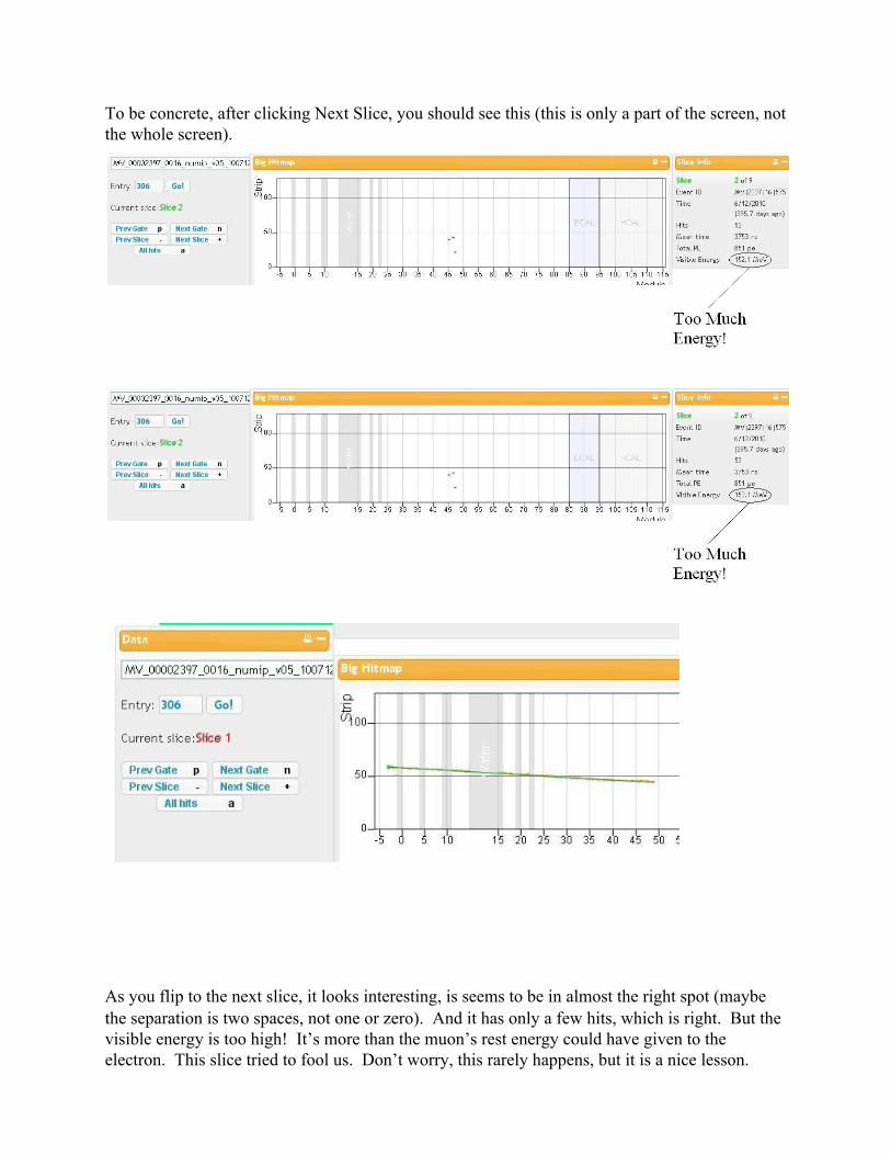
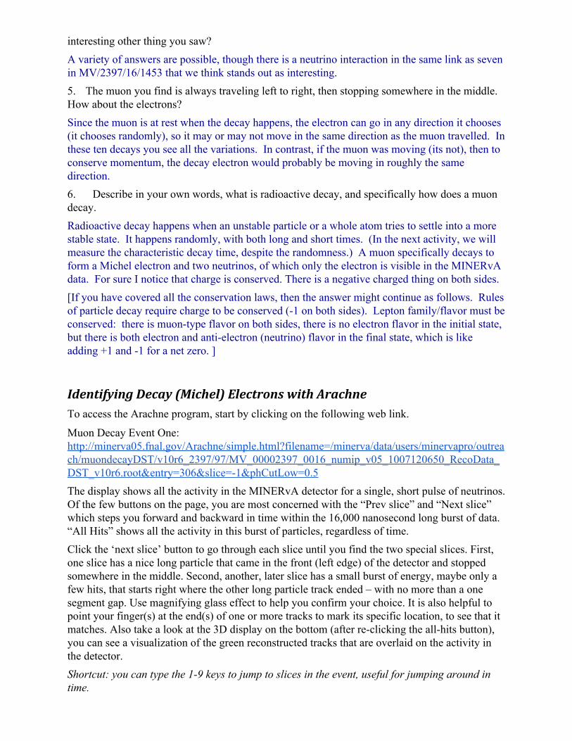
To be concrete, after clicking Next Slice, you should see this (this is only a part of the screen, not the whole screen).

As you flip to the next slice, it looks interesting, is seems to be in almost the right spot (maybe the separation is two spaces, not one or zero). And it has only a few hits, which is right. But the visible energy is too high! It’s more than the muon’s rest energy could have given to the electron. This slice tried to fool us. Don’t worry, this rarely happens, but it is a nice lesson.

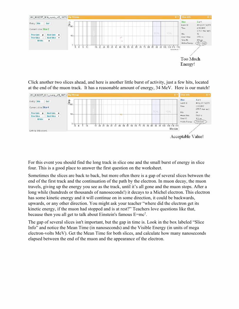
Click another two slices ahead, and here is another little burst of activity, just a few hits, located at the end of the muon track. It has a reasonable amount of energy, 34 MeV. Here is our match!

For this event you should find the long track in slice one and the small burst of energy in slice four. This is a good place to answer the first question on the worksheet. Sometimes the slices are back to back, but more often there is a gap of several slices between the end of the first track and the continuation of the path by the electron. In muon decay, the muon travels, giving up the energy you see as the track, until it’s all gone and the muon stops. After a long while (hundreds or thousands of nanoseconds!) it decays to a Michel electron. This electron has some kinetic energy and it will continue on in some direction, it could be backwards, upwards, or any other direction. You might ask your teacher “where did the electron get its kinetic energy, if the muon had stopped and is at rest?” Teachers love questions like that, because then you all get to talk about Einstein's famous E=mc2. The gap of several slices isn't important, but the gap in time is. Look in the box labeled “Slice Info” and notice the Mean Time (in nanoseconds) and the Visible Energy (in units of mega electron­volts MeV). Get the Mean Time for both slices, and calculate how many nanoseconds elapsed between the end of the muon and the appearance of the electron.

In the “Slice Info” box, also, get the Visible Energy for the electron from the decay. It is expected that the electron can carry between zero MeV and up to half the energy of the muon at rest, which is 107 MeV. The other energy is carried off, unseen, by two neutrinos. The final distinguishing feature of muon decay is this energy, which should be less than 60 MeV. If you think you have a splash that matches (using your finger on the screen) in space, but has more energy than this, it indicates something other than muon decay. Look for the mean time value in the Slice information box for slice 1. That data is already entered in the appropriate data slot. We have also done that for slice 4. Note that for slice 4 you will also need the visible energy value. Subtract the mean time for the muon slice (slice 1) from the mean time for the electron slice (slice 4), in this example you get 1410 nanoseconds. Check that the data recorded on your data table matches what is shown on the Arachne screen for each slice. The final thing you should get from the slice box is the Event ID which is MV/2397/16/575. This is a unique identification number, so you can use it to make sure you know which events you are talking about and not get them mixed up with others. Now we can get started looking at nine more pulses of the beam at Fermilab. Go one by one through the following nine links to find the muon and its decay electron. There is one pair in each of these nine. Muon Decay Event Two: http://minerva05.fnal.gov/Arachne/simple.html?filename=/minerva/data/users/minervapro/outreach/muondecayDST/v10r6_2397/97/MV_00002397_0016_numip_v05_1007120650_RecoData_DST_v10r6.root&entry=344&slice=­1&phCutLow=0.5 Muon Decay Event Three: http://minerva05.fnal.gov/Arachne/simple.html?filename=/minerva/data/users/minervapro/outreach/muondecayDST/v10r6_2397/97/MV_00002397_0016_numip_v05_1007120650_RecoData_DST_v10r6.root&entry=456&slice=­1&phCutLow=0.5 Muon Decay Event Four: http://minerva05.fnal.gov/Arachne/simple.html?filename=/minerva/data/users/minervapro/outreach/muondecayDST/v10r6_2397/97/MV_00002397_0016_numip_v05_1007120650_RecoData_

DST_v10r6.root&entry=469&slice=­1&phCutLow=0.5 Muon Decay Event Five: http://minerva05.fnal.gov/Arachne/simple.html?filename=/minerva/data/users/minervapro/outreach/muondecayDST/v10r6_2397/97/MV_00002397_0016_numip_v05_1007120650_RecoData_DST_v10r6.root&entry=496&slice=­1&phCutLow=0.5 Muon Decay Event Six: http://minerva05.fnal.gov/Arachne/simple.html?filename=/minerva/data/users/minervapro/outreach/muondecayDST/v10r6_2397/97/MV_00002397_0016_numip_v05_1007120650_RecoData_DST_v10r6.root&entry=668&slice=­1&phCutLow=0.5 Muon Decay Event Seven: http://minerva05.fnal.gov/Arachne/simple.html?filename=/minerva/data/users/minervapro/outreach/muondecayDST/v10r6_2397/97/MV_00002397_0016_numip_v05_1007120650_RecoData_DST_v10r6.root&entry=786&slice=­1&phCutLow=0.5 Muon Decay Event Eight: http://minerva05.fnal.gov/Arachne/simple.html?filename=/minerva/data/users/minervapro/outreach/muondecayDST/v10r6_2397/97/MV_00002397_0017_numip_v05_1007120720_RecoData_DST_v10r6.root&entry=157&slice=­1&phCutLow=0.5 Muon Decay Event Nine: http://minerva05.fnal.gov/Arachne/simple.html?filename=/minerva/data/users/minervapro/outreach/muondecayDST/v10r6_2397/97/MV_00002397_0017_numip_v05_1007120720_RecoData_DST_v10r6.root&entry=502&slice=­1&phCutLow=0.5 Muon Decay Event Ten:: http://minerva05.fnal.gov/Arachne/simple.html?filename=/minerva/data/users/minervapro/outreach/muondecayDST/v10r6_2397/97/MV_00002397_0017_numip_v05_1007120720_RecoData_DST_v10r6.root&entry=536&slice=­1&phCutLow=0.5

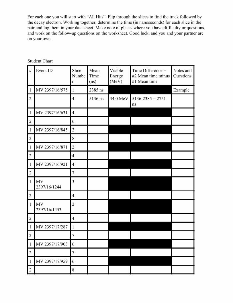
For each one you will start with “All Hits”. Flip through the slices to find the track followed by the decay electron. Working together, determine the time (in nanoseconds) for each slice in the pair and log them in your data sheet. Make note of places where you have difficulty or questions, and work on the follow­up questions on the worksheet. Good luck, and you and your partner are on your own. Student Chart

# Event ID Slice Number

Mean Time (ns)

Visible Energy (MeV)

Time Difference = #2 Mean time minus #1 Mean time

Notes and Questions

1 MV 2397/16/575 1 2385 ns Example

2 4 5136 ns 34.0 MeV 5136­2385 = 2751 ns

1 MV 2397/16/631 4

2 6

1 MV 2397/16/845 2

2 8

1 MV 2397/16/871 2

2 4

1 MV 2397/16/921 4

2 7

1 MV 2397/16/1244

3

2 4

1 MV 2397/16/1453

2

2 4

1 MV 2397/17/287 1

2 7

1 MV 2397/17/903 6

2 7

1 MV 2397/17/959 6

2 8

Questions from activity Getting started finding muon decays 1. As you flip through the time­slices of Muon Decay Event One, how many have activity

that is track­like? How many are small splashes of energy? 2. There were actually two time­slices in Event One, each with a small splash, which

occurred at the end of the muon track. How did you know which one was the decay electron and which one to reject as some other unrelated thing?

3. Considering all eleven links, which one has the most time between the decay electron and its parent particle? Which one has the least time?

4. In addition to all the muons that stopped in the middle and decayed, what was the most interesting other thing you saw?

5. The muon you find is always traveling left to right, then stopping somewhere in the middle. How about the electrons?

6. Describe in your own words, what is radioactive decay, and specifically how does a muon decay.

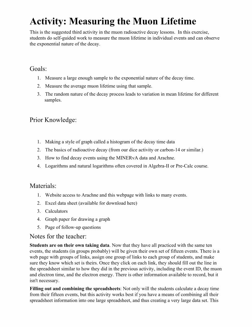
Activity: Measuring the Muon Lifetime This is the suggested third activity in the muon radioactive decay lessons. In this exercise, students do self­guided work to measure the muon lifetime in individual events and can observe the exponential nature of the decay.

Goals: 1. Measure a large enough sample to the exponential nature of the decay time. 2. Measure the average muon lifetime using that sample. 3. The random nature of the decay process leads to variation in mean lifetime for different

samples.

Prior Knowledge:

1. Making a style of graph called a histogram of the decay time data 2. The basics of radioactive decay (from our dice activity or carbon­14 or similar.) 3. How to find decay events using the MINERvA data and Arachne. 4. Logarithms and natural logarithms often covered in Algebra­II or Pre­Calc course.

Materials: 1. Website access to Arachne and this webpage with links to many events. 2. Excel data sheet (available for download here) 3. Calculators 4. Graph paper for drawing a graph 5. Page of follow­up questions

Notes for the teacher: Students are on their own taking data. Now that they have all practiced with the same ten events, the students (in groups probably) will be given their own set of fifteen events. There is a web page with groups of links, assign one group of links to each group of students, and make sure they know which set is theirs. Once they click on each link, they should fill out the line in the spreadsheet similar to how they did in the previous activity, including the event ID, the muon and electron time, and the electron energy. There is other information available to record, but it isn't necessary. Filling out and combining the spreadsheets: Not only will the students calculate a decay time from their fifteen events, but this activity works best if you have a means of combining all their spreadsheet information into one large spreadsheet, and thus creating a very large data set. This

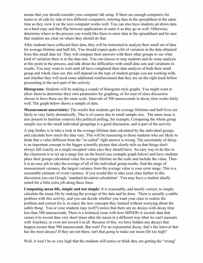
means that you should consider your computer lab setup. If there are enough computers for teams to sit side by side at two different computers, entering data in the spreadsheet at the same time as they view it on the next computer works well. You can also have students jot down data on a hard copy and then flip between applications to enter it as they go as well. Otherwise, determine where in the process you would like them to enter data in the spreadsheet and be sure that students are clear on where they should do that. After students have collected their data, they will be instructed to analyze their small set of data for average lifetime and half­life. You should expect quite a bit of variation in the data obtained from this small data set. They will compare their answers with three other groups to see what kind of variation there is in the data sets. You can choose to stop students and do some analysis at this point in the process, and talk about the difficulties with small data sets and variations in results. You may want to wait until all have completed their data analysis of both their small group and whole class set, this will depend on the type of student groups you are working with, and whether they will need some additional reinforcement that they are on the right track before proceeding to the next part of the activity. Histograms: Students will be making a couple of histogram style graphs. You might want to allow them to determine their own parameters for graphing, or for ease of class discussion choose to have them use the same scale. Intervals of 500 nanoseconds in decay time works fairly well. The graph below shows a sample of data. Measurement uncertainty: The results that students get for average lifetimes and half­lives are likely to vary fairly dramatically. This is of course due to small sample size. The same issue is also present in familiar contexts like political polling, for example. Comparing the whole group sample size to the small individual groupings is a good discussion, and is part of the activity. A step further is to take a look at the average lifetime data calculated by the individual groups, and calculate how much the data vary. This will be reassuring to those students who are likely to think that a value different from the “so called” right answer is wrong. The uncertainty of decay is an important concept in the bigger scientific picture that clearly tells us that things don't always fall exactly as a single accepted value says they should have. An easy way to do this in the classroom is to set up a range line on the board (see example graph below) and have students place their groups calculated value for average lifetime on the scale and include the value. Then it is an easy job to take the average of all of the individual group results, find the range of measurement variance, the largest variance from the average value is your error range. This is a reasonable estimate of event variance. If you would like to take your class further in this discussion you can Google ‘standard deviation calculation’. You may have a student ideally suited for a little extra job along these lines. Computing mean life, simple and not simple: It is reasonable, and mostly correct, to simply calculate the mean life by making the average of the data and be done. There is actually a subtle problem with this activity, and you can decide whether you want your class to realize the problem and correct for it, or enjoy the new concepts they learned without worrying about the subtle thing. You or your students may (will?) notice that there are no decays with decay time less than 500 nanoseconds. There is a technical issue with how MINERvA records data that causes it to record data very short times after the muon in a different way (that we can't measure with Arachne), or even not record it at all. Because of this, we have hidden any decays that happen sooner than 500 nanoseconds. But wait! For an exponential decay, that’s the interval that has the most decays! If they are not there, isn't that going to make our mean life too high? Well, it won’t be so very high that the students will notice or think they are getting the “wrong”

answer. So no harm is done? Or you can consider two ways of correcting it. The boring but effective way, but one that is often used by practicing scientists, is to estimate what events were missing from that first interval, include that estimate into your average, and consider that the more accurate number with some uncertainty because your estimate probably wasn’t perfect. Okay, this is totally valid, as long as you include that in your discussion of the results. The interesting argument that leads to a correction to the average lifetime invokes an understanding of the dice activity in a very special way. If you want your students to try it, cut and paste the following thing into the instructions and questions for your students. [For students: if the teacher wants them to consider it.] There is a problem here, there is data missing between 0 and 500 ns. That’s actually the interval where we expect most of the events to be, so our average will be too high by a little bit. But the fix is interesting. Remember the dice activity, especially the version where you threw 100 dice at the same time, and separated out those with a “one”, and then rolled again? Each time you rolled, it was the same random 1/6 chance, the dice don’t remember how many rolls went by without decaying. You could have ignored that first roll, and just as well pretended you had started out with roughly 85 dice. Or maybe you didn’t know it, but there was a prior roll you didn’t see that had 115 dice, and you walked in with only 100 left. Your analysis of the lifetime for the dice wouldn’t have been affected by it. Likewise, we can analyze the average lifetime of the muons as if those that decayed in the first interval never happened, and the lifetime clock started 500 nanoseconds later, for the second roll. If this is convincing, then mathematically we have two (equivalent) choices. Either subtract 500 nanoseconds from every event we are putting into the mean lifetime calculation, or subtract 500 nanoseconds from the average. Do you see that these two are equivalent? If you do, then the latter choice is easier, and will give you a more accurate measurement. Looking at only student small group results should result in an average lifetime for muons of 2.29 μs. Note this is converted from the nanoseconds used in the graphing activity to microseconds­ just move the decimal three places to the left. The average muon half­life should be somewhere in the range of 1.56 μs. If all of the student groups’ average time difference is calculated we get a range of times from 1.591 to 3.079 μs. The largest difference is 0.793 μs providing the error range for this set of data. The next step asks students to make the same calculations using the whole group data. The data yields 2.32 μs for the average lifetime in this scenario, and an half­life of 1.61 μs. Graphs below for time difference, show the distribution for the assigned group data at the time of writing this guide.

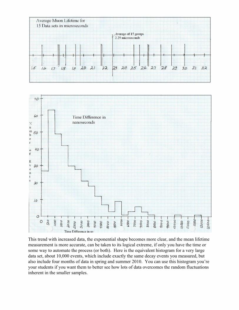
This trend with increased data, the exponential shape becomes more clear, and the mean lifetime measurement is more accurate, can be taken to its logical extreme, if only you have the time or some way to automate the process (or both). Here is the equivalent histogram for a very large data set, about 10,000 events, which include exactly the same decay events you measured, but also include four months of data in spring and summer 2010. You can use this histogram you’re your students if you want them to better see how lots of data overcomes the random fluctuations inherent in the smaller samples.

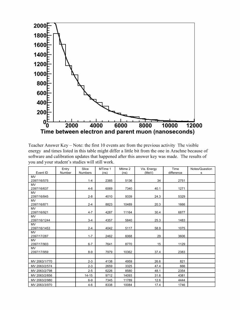
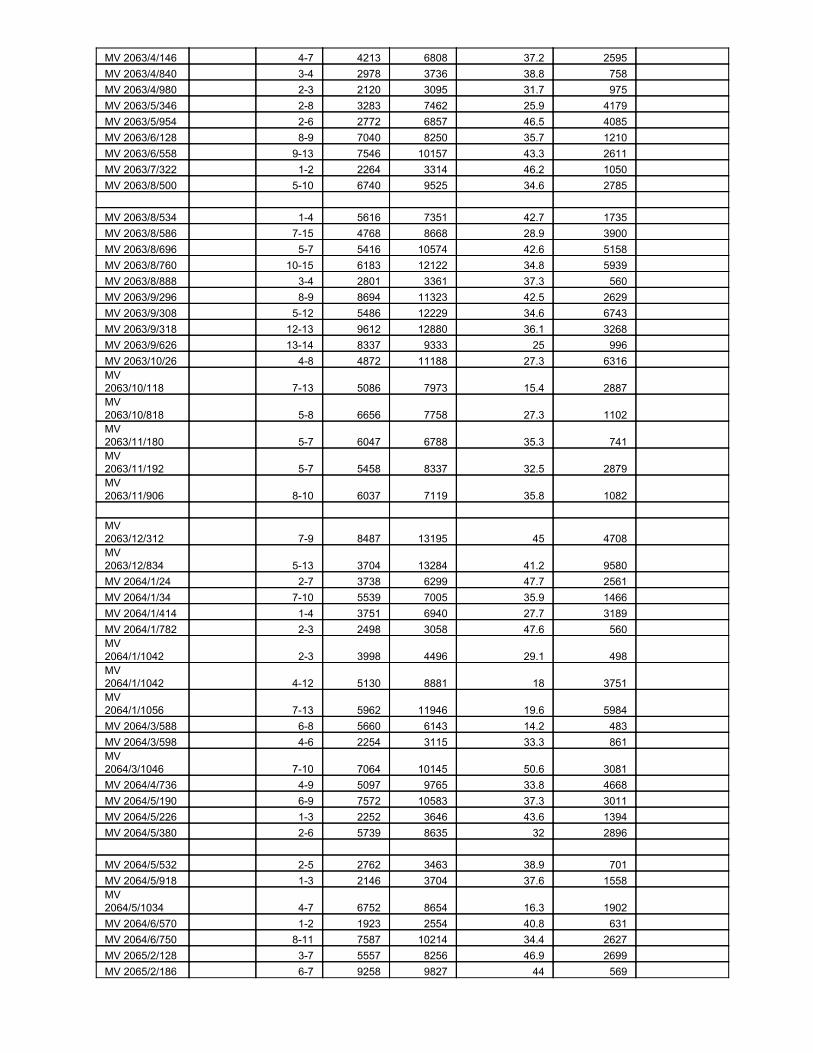
Teacher Answer Key – Note: the first 10 events are from the previous activity The visible energy and times listed in this table might differ a little bit from the one in Arachne because of software and calibration updates that happened after this answer key was made. The results of you and your student’s studies will still work.

Event ID Entry Number

Slice Numbers

MTime 1 (ns)

Mtime 2 (ns)

Vis. Energy (MeV)

Time difference

Notes/Questions

MV 2397/16/575 1­4 2385 5136 34 2751 MV 2397/16/637 4­6 6069 7340 40.1 1271 MV 2397/16/845 2­8 4010 9339 24.3 5329 MV 2397/16/871 2­4 8823 10489 20.3 1666 MV 2397/16/921 4­7 4287 11164 30.4 6877 MV 2397/16/1244 3­4 4357 5840 25.3 1483 MV 2397/16/1453 2­4 4042 5117 58.9 1075 MV 2397/17/287 1­7 2462 6068 29 3606 MV 2397/17/903 6­7 7641 8770 15 1129 MV 2397/17/959 8­9 7979 10362 37.4 2383 MV 2063/1/770 2­3 4138 4959 26.6 821 MV 2063/2/574 2­3 2659 3325 47.4 666 MV 2063/2/798 2­5 6226 8580 48.1 2354 MV 2063/2/856 14­15 9712 14093 31.6 4381 MV 2063/2/980 6­9 7345 11789 12.6 4444 MV 2063/3/970 4­6 8338 10084 17.4 1746

MV 2063/4/146 4­7 4213 6808 37.2 2595 MV 2063/4/840 3­4 2978 3736 38.8 758 MV 2063/4/980 2­3 2120 3095 31.7 975 MV 2063/5/346 2­8 3283 7462 25.9 4179 MV 2063/5/954 2­6 2772 6857 46.5 4085 MV 2063/6/128 8­9 7040 8250 35.7 1210 MV 2063/6/558 9­13 7546 10157 43.3 2611 MV 2063/7/322 1­2 2264 3314 46.2 1050 MV 2063/8/500 5­10 6740 9525 34.6 2785 MV 2063/8/534 1­4 5616 7351 42.7 1735 MV 2063/8/586 7­15 4768 8668 28.9 3900 MV 2063/8/696 5­7 5416 10574 42.6 5158 MV 2063/8/760 10­15 6183 12122 34.8 5939 MV 2063/8/888 3­4 2801 3361 37.3 560 MV 2063/9/296 8­9 8694 11323 42.5 2629 MV 2063/9/308 5­12 5486 12229 34.6 6743 MV 2063/9/318 12­13 9612 12880 36.1 3268 MV 2063/9/626 13­14 8337 9333 25 996 MV 2063/10/26 4­8 4872 11188 27.3 6316 MV 2063/10/118 7­13 5086 7973 15.4 2887 MV 2063/10/818 5­8 6656 7758 27.3 1102 MV 2063/11/180 5­7 6047 6788 35.3 741 MV 2063/11/192 5­7 5458 8337 32.5 2879 MV 2063/11/906 8­10 6037 7119 35.8 1082 MV 2063/12/312 7­9 8487 13195 45 4708 MV 2063/12/834 5­13 3704 13284 41.2 9580 MV 2064/1/24 2­7 3738 6299 47.7 2561 MV 2064/1/34 7­10 5539 7005 35.9 1466 MV 2064/1/414 1­4 3751 6940 27.7 3189 MV 2064/1/782 2­3 2498 3058 47.6 560 MV 2064/1/1042 2­3 3998 4496 29.1 498 MV 2064/1/1042 4­12 5130 8881 18 3751 MV 2064/1/1056 7­13 5962 11946 19.6 5984 MV 2064/3/588 6­8 5660 6143 14.2 483 MV 2064/3/598 4­6 2254 3115 33.3 861 MV 2064/3/1046 7­10 7064 10145 50.6 3081 MV 2064/4/736 4­9 5097 9765 33.8 4668 MV 2064/5/190 6­9 7572 10583 37.3 3011 MV 2064/5/226 1­3 2252 3646 43.6 1394 MV 2064/5/380 2­6 5739 8635 32 2896 MV 2064/5/532 2­5 2762 3463 38.9 701 MV 2064/5/918 1­3 2146 3704 37.6 1558 MV 2064/5/1034 4­7 6752 8654 16.3 1902 MV 2064/6/570 1­2 1923 2554 40.8 631 MV 2064/6/750 8­11 7587 10214 34.4 2627 MV 2065/2/128 3­7 5557 8256 46.9 2699 MV 2065/2/186 6­7 9258 9827 44 569

MV 2065/2/526 2­8 6924 11125 31.2 4201 MV 2065/2/544 2­6 3235 5947 45.7 2712 MV 2065/3/422 2­5 2573 3722 46.4 1149 MV 2065/3/594 12­13 9162 10388 42.5 1226 MV 2065/3/904 3­7 2906 6765 24.4 3859 MV 2065/3/998 8­13 7266 11733 44.1 4467 MV 2067/1/116 1­6 2164 4396 22.7 2232 MV 2067/1/320 7­11 6288 12499 28.7 6211 MV 2067/1/1010 6­7 7635 12222 45.7 4587 MV 2067/2/154 1­4 2738 4259 33.1 1521 MV 2067/2/706 6­11 5513 12303 40.1 6790 MV 2067/3/84 1­7 2045 13224 28.9 11179 MV 2067/3/276 11­15 7741 9896 12.2 2155 MV 2067/4/740 4­8 5083 8097 25.5 3014 MV 2067/4/1014 4­7 5870 7501 26.3 1631 MV 2067/4/1108 3­4 5983 6501 45.3 518 MV 2067/4/1164 1­6 3013 6925 47.2 3912 MV 2067/5/108 10­11 9353 12744 13.7 3391 MV 2067/5/748 8­9 7473 9496 36.1 2023 MV 2067/6/226 3­4 7995 8498 36.7 503 MV 2067/6/606 2­5 2336 3498 40.3 1162 MV 2067/6/690 1­2 2355 2907 28.4 552 MV 2067/6/832 3­6 7258 14557 31 7299 MV 2067/6/1060 11­13 8524 11992 45.4 3468 MV 2067/7/216 1­2 1861 2394 27.9 533 MV 2067/8/788 6­8 7243 10829 41.4 3586 MV 2067/68/802 6­7 7393 13841 35 6448 MV 2067/8/924 2­10 3567 7707 21.9 4140 MV 2067/8/976 7­8 7693 10347 16.9 2654 MV 2067/9/86 10­11 7116 7955 30.2 839 MV 2067/9/174 9­11 8330 9711 26.2 1381 MV 2067/89/220 8­11 5663 7431 22.1 1768 MV 2067/9/718 8­10 7503 11474 15.8 3971 MV 20679/760 4­5 5201 6722 27.5 1521 MV 2067/10/146 12­14 7468 13814 48.4 6346 MV 2067/10/1048 5­8 4142 7390 39.5 673 MV 2067/10/1152 5­7 4712 7939 26.7 3227 MV 2067/11//90 9­12 7887 10961 39.7 3074 MV 2067/11/872 6­8 5491 6115 21.7 624 MV 2067/11/896 4­6 5491 8458 32.4 2967 MV 2067/11/896 2­8 3447 9891 7.6 6444 MV 2067/12/92 1­5 2158 4757 40.6 2599 MV 2067/12/92 2­4 2768 4174 17.4 1406 MV 2067/12/322 6­7 8977 9815 35.6 838 MV 2067/13/2 4­5 4491 5138 35.1 647 MV 4­8 5613 15026 20.1 9413

2067/13/268 MV 2067/13/448 5­10 6663 10384 19.2 3721 MV 2067/13/490 3­8 4384 7466 35.6 3082 MV 2067/13/514 6­12 5819 8295 29 2476 MV 2067/13/826 6­7 6286 6787 43.2 501 MV 2067/14/274 1­2 2526 3652 25 1126 MV 2067/14/448 6­8 5928 8161 40 2233 MV 2067/14/522 4­5 4260 4788 36.2 528 MV 2067/14/1074 3­7 3035 5107 35.6 2072 MV 2067/15/188 2­5 5371 8130 34.9 2759 MV 2067/15/694 11­12 8768 10287 41.3 1519 MV 2067/15/842 4­7 4879 6243 21.6 1364 MV 2067/15/1014 4­9 5702 10800 11.6 5098 MV 2067/15/1034 3­4 2731 3910 26.7 1179 MV 2067/16/394 6­8 7578 8392 18.5 814 MV 2067/16/488 1­4 2963 4445 30.2 1482 MV 2067/16/518 5­7 5661 7076 55.4 1415 MV 2067/17/272 5­7 6280 12780 32.3 6500 MV 2067/17/606 2­7 2458 8136 35.4 5678 MV 2071/1/6 5­9 7035 10443 44.9 3408 MV 2071/1/1004 2­4 2332 4095 16.6 1763 MV 2071/2/58 8­9 9502 10134 32.8 632 MV 2071/2/498 3­5 6057 6615 24.2 558 MV 2071/3/162 7­8 7331 8965 32 1634 MV 2071/3/258 4­6 4042 4637 12.4 595 MV 2071/3/258 5­7 4477 5548 21.3 1071 MV 2071/3/818 2­3 3106 3975 43.5 869 MV 2071/3/1064 8­11 6826 9231 17.7 2405 MV 2071/4/64 3­9 2549 6577 25.2 4028 MV 2071/4/404 1­2 1882 2658 14.1 776 MV 2071/4/404 9­10 9259 9963 10.1 704 MV 2071/4/640 1­5 3185 5624 56.8 2439 MV 2071/4/726 4­5 8001 9526 43.8 1525 MV 2071/5/54/ 3­6 6384 9031 29.6 2647 MV 2071/5/1104 3­5 6401 7029 46.8 628 MV 2071/6/372 6­8 5372 6780 29.6 1408 MV 2071/6/476 6­7 6213 7368 47.7 1155 MV 2071/6/498 3­4 2660 4756 32.3 2096 MV 2071/6/818 2­5 3425 6038 14.8 2613 MV 2071/6/1032 7­9 6928 7771 30.9 843 MV 2071/6/1148 6­10 6354 8526 41.4 2172

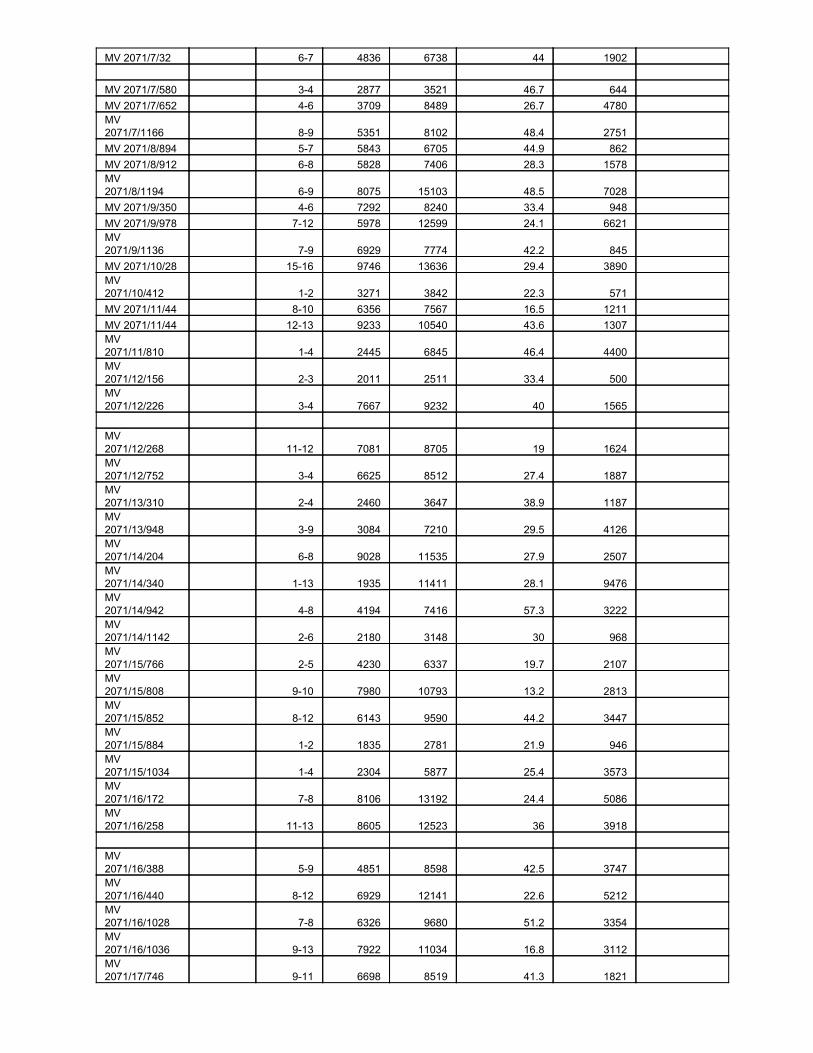
MV 2071/7/32 6­7 4836 6738 44 1902 MV 2071/7/580 3­4 2877 3521 46.7 644 MV 2071/7/652 4­6 3709 8489 26.7 4780 MV 2071/7/1166 8­9 5351 8102 48.4 2751 MV 2071/8/894 5­7 5843 6705 44.9 862 MV 2071/8/912 6­8 5828 7406 28.3 1578 MV 2071/8/1194 6­9 8075 15103 48.5 7028 MV 2071/9/350 4­6 7292 8240 33.4 948 MV 2071/9/978 7­12 5978 12599 24.1 6621 MV 2071/9/1136 7­9 6929 7774 42.2 845 MV 2071/10/28 15­16 9746 13636 29.4 3890 MV 2071/10/412 1­2 3271 3842 22.3 571 MV 2071/11/44 8­10 6356 7567 16.5 1211 MV 2071/11/44 12­13 9233 10540 43.6 1307 MV 2071/11/810 1­4 2445 6845 46.4 4400 MV 2071/12/156 2­3 2011 2511 33.4 500 MV 2071/12/226 3­4 7667 9232 40 1565 MV 2071/12/268 11­12 7081 8705 19 1624 MV 2071/12/752 3­4 6625 8512 27.4 1887 MV 2071/13/310 2­4 2460 3647 38.9 1187 MV 2071/13/948 3­9 3084 7210 29.5 4126 MV 2071/14/204 6­8 9028 11535 27.9 2507 MV 2071/14/340 1­13 1935 11411 28.1 9476 MV 2071/14/942 4­8 4194 7416 57.3 3222 MV 2071/14/1142 2­6 2180 3148 30 968 MV 2071/15/766 2­5 4230 6337 19.7 2107 MV 2071/15/808 9­10 7980 10793 13.2 2813 MV 2071/15/852 8­12 6143 9590 44.2 3447 MV 2071/15/884 1­2 1835 2781 21.9 946 MV 2071/15/1034 1­4 2304 5877 25.4 3573 MV 2071/16/172 7­8 8106 13192 24.4 5086 MV 2071/16/258 11­13 8605 12523 36 3918 MV 2071/16/388 5­9 4851 8598 42.5 3747 MV 2071/16/440 8­12 6929 12141 22.6 5212 MV 2071/16/1028 7­8 6326 9680 51.2 3354 MV 2071/16/1036 9­13 7922 11034 16.8 3112 MV 2071/17/746 9­11 6698 8519 41.3 1821

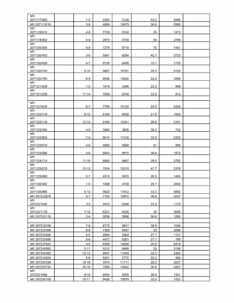
MV 2071/17/950 1­5 2283 5129 53.5 2846 MV 2071/18/16 3­8 4689 10679 36.6 5990 MV 2071/18/412 4­6 7729 9142 25 1413 MV 2071/18/952 4­9 2970 5759 50 2789 MV 2071/20/304 6­8 7279 8710 15 1431 MV 2071/20/402 3­6 5561 8284 42.7 2723 MV 2071/20/458 4­7 6726 8456 15.7 1730 MV 2071/20/702 5­15 5667 10791 35.4 5124 MV 2071/20/764 8­9 9536 12920 22.6 3384 MV 2071/21/208 1­2 1818 2486 22.3 668 MV 2071/21/208 11­14 7939 8749 22.8 810 MV 2071/21/634 6­7 7795 10120 24.4 2325 MV 2071/22/116 9­10 6100 8030 21.6 1930 MV 2071/22/116 13­14 9180 12341 26.8 3161 MV 2071/22/494 4­5 3084 3826 38.2 742 MV 2071/22/804 7­9 9014 11316 32.9 2302 MV 2071/23/618 4­6 4800 5656 41 856 MV 2071/23/586 4­6 6943 8915 38.8 1972 MV 2071/24/714 11­16 6685 9467 29.5 2782 MV 2071/25/276 10­12 7934 10310 47.7 2376 MV 2071/25/680 5­7 4515 5970 26.5 1455 MV 2071/26/382 1­5 1898 4728 29.7 2830 MV 2071/26/886 5­12 5620 11612 33.3 5992 MV 2072/2/878 5­7 7745 10972 38.8 3227 MV 2072/2/1042 3­5 4033 5208 23.2 1175 MV 2072/2/1178 7­14 6221 9226 30 3005 MV 2072/3/118 2­4 2636 3896 56.6 1260 MV 2072/3/238 7­8 8772 9817 30.8 1045 MV 2072/3/306 6­8 7359 9457 33 2098 MV 2072/3/426 2­5 2954 5402 27.7 1137 MV 2072/3/580 5­6 4472 5261 27.7 789 MV 2072/3/922 4­5 8359 14838 25.5 6479 MV 2072/4/582 5­11 5312 8468 33 3156 MV 2072/4/582 12­13 9047 11409 33.3 2362 MV 2072/4/624 5­6 5201 5770 22.2 569 MV 2072/5/336 15­18 7874 11111 26.2 3237 MV 2072/5/734 16­19 7985 10442 35.6 2457 MV 2072/5/1056 8­10 6954 8305 26.4 1351 MV 2072/6/108 10­11 9426 10979 32.6 1553

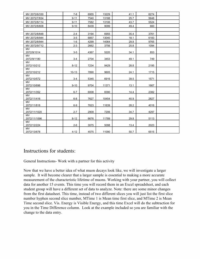
MV 2072/6/330 7­8 6955 13229 41.1 6274 MV 2072/7/834 9­11 7540 13188 25.7 5648 MV 2072/8/114 9­11 7582 13106 43.7 5524 MV 2072/8/608 9­10 8439 9099 49.4 660 MV 2072/8/848 2­4 3194 6955 35.4 3761 MV 2072/8/944 3­5 6857 13040 18.1 6183 MV 2072/8/944 1­6 4299 14064 29.8 9765 MV 2072/9/712 2­3 2662 3756 25.8 1094 MV 2072/9/1014 3­5 4367 5220 34.1 853 MV 2072/9/1180 3­4 2704 3453 49.1 749 MV 2072/10/212 8­12 7234 9429 28.8 2195 MV 2072/10/212 10­13 7890 9605 24.1 1715 MV 2072/10/572 3­4 5345 6916 39.5 1571 MV 2072/10/698 9­10 9704 11371 13.1 1667 MV 2072/11/352 6­7 6008 8390 14.4 2382 MV 2072/11/416 6­8 7627 10454 40.9 2827 MV 2072/11/818 6­9 7623 11639 28.2 4016 MV 2072/11/1020 2­7 2909 7206 34.7 4297 MV 2072/11/1096 8­12 6676 11789 29.8 5113 MV 2072/12/224 2­6 3075 5098 13.4 2023 MV 2072/13/678 4­12 4575 11090 50.7 6515

Instructions for students: General Instructions­ Work with a partner for this activity Now that we have a better idea of what muon decays look like, we will investigate a larger sample. It will become clearer that a larger sample is essential to making a more accurate measurement of the characteristic lifetime of muons. Working with your partner, you will collect data for another 15 events. This time you will record them in an Excel spreadsheet, and each student group will have a different set of data to analyze. Note: there are some minor changes from the first datasheet. This time, instead of two different slices you will just list the first slice number hyphen second slice number, MTime 1 is Mean time first slice, and MTime 2 is Mean Time second slice. Vis. Energy is Visible Energy, and this time Excel will do the subtraction for you in the Time Difference column. Look at the example included so you are familiar with the change to the data entry.

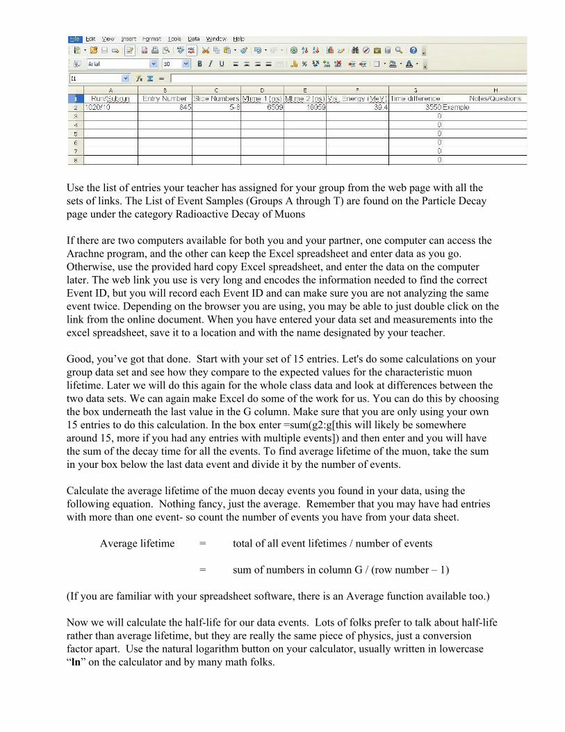
Use the list of entries your teacher has assigned for your group from the web page with all the sets of links. The List of Event Samples (Groups A through T) are found on the Particle Decay page under the category Radioactive Decay of Muons If there are two computers available for both you and your partner, one computer can access the Arachne program, and the other can keep the Excel spreadsheet and enter data as you go. Otherwise, use the provided hard copy Excel spreadsheet, and enter the data on the computer later. The web link you use is very long and encodes the information needed to find the correct Event ID, but you will record each Event ID and can make sure you are not analyzing the same event twice. Depending on the browser you are using, you may be able to just double click on the link from the online document. When you have entered your data set and measurements into the excel spreadsheet, save it to a location and with the name designated by your teacher. Good, you’ve got that done. Start with your set of 15 entries. Let's do some calculations on your group data set and see how they compare to the expected values for the characteristic muon lifetime. Later we will do this again for the whole class data and look at differences between the two data sets. We can again make Excel do some of the work for us. You can do this by choosing the box underneath the last value in the G column. Make sure that you are only using your own 15 entries to do this calculation. In the box enter =sum(g2:g[this will likely be somewhere around 15, more if you had any entries with multiple events]) and then enter and you will have the sum of the decay time for all the events. To find average lifetime of the muon, take the sum in your box below the last data event and divide it by the number of events. Calculate the average lifetime of the muon decay events you found in your data, using the following equation. Nothing fancy, just the average. Remember that you may have had entries with more than one event­ so count the number of events you have from your data sheet.

Average lifetime = total of all event lifetimes / number of events

= sum of numbers in column G / (row number – 1) (If you are familiar with your spreadsheet software, there is an Average function available too.) Now we will calculate the half­life for our data events. Lots of folks prefer to talk about half­life rather than average lifetime, but they are really the same piece of physics, just a conversion factor apart. Use the natural logarithm button on your calculator, usually written in lowercase “ln” on the calculator and by many math folks.

Half­life = Average lifetime x ln 2

This one we don't need Excel to do the work for us­ just a calculator with a natural log function on it. Take the average lifetime you determined and multiple it by the natural log of 2 (which is about .693). This simplified equation has its roots with the following expression which describes exponential decay.

If you let No be 1.0, it describes the probability that the muon will still be there after some amount of time t. Try it out with your calculator, which has an ex button. put τmean = 2.2 microseconds and try a few values for t between 0.5 and 10 microseconds and write down the answers here in the margin of this page. Don't forget the minus sign in the exponent! If you plotted the result for these different test values, what would the graph look like? As you finish your calculations keep track of the data you collected here and compare results with other groups as they complete their data. Your teacher will be asking the class to compare your individual small group results for lifetime and half­life. Hey, wait! We just calculated something that has a funny name. What does the half­life mean? Notice the range of time differences in your list. Some are very long, many thousands of nanoseconds. Some are quite short, just a few hundred nanoseconds. The mean lifetime is the average of those. The half­life is the amount of time after which half the muons have decayed and half have not. Compare the number you calculated to the list of time differences and see if that is approximately right. The comparison might not be exact, but it should be very close. If it is not close, double check your calculation. If it looks good after double checking your work, then congratulations! You just made a measurement of the half­life of the muon. When all groups have completed entering their data and saving it, the next step will involve working with the whole class data set, as well as your own 15 entries. If there is wait time for other groups to complete their data entry, this is a good time to work on the follow­up questions from this round of analysis. OK, so now you should have access to an Excel file that has the entire class data set, as well as your own group’s 15 entries. We want the larger number of events for the graphing portion of the lab. The Excel file will likely be in a read only form. Open it up, copy and paste the entire set into a new Excel document so you can modify it without messing up the original. This one you will be able to manipulate to organize data. This keeps a safe set of data available for everyone just in case there are any accidents as you manipulate the data table. Save your new one. We are going to graph visible energy first. On the Excel spreadsheet sort your data by column F, or the visible energy data. When you choose sort, be sure that all the data in the table is highlighted. Sometimes the program does this automatically, sometimes you need to highlight everything before you choose sort from the menu. Choose ascending order on the right side. This should move all the data in order according to visible energy.

Look at the data and determine the range of data and how you will organize it on your graph. Number of events will be the y axis, and visible energy in MeV will be the x axis on your graph. Set your graph up so it occupies as much of the page as possible. You will be making a histogram graph with a bar representing the data rather than a point. You will need to set up your own range of measurements. For ease of discussion, your teacher may give you a specified range. While someone in the class is finishing putting all of the class's data together, let's step back and think about the kind of graph we are going to make. We're going to make something called a histogram. Let's look at a histogram of some data you are more familiar with. The graph here is an example of an event histogram designed to provide a visualization of a range of occurrences of a particular type of event. This is a histogram of the number of hurricanes

which were large enough in the Atlantic Ocean to earn a name between the years of 1990 to present. Can you see a trend in the data? What can you summarize from the data as it is presented? If you had to predict the number of hurricanes in the next two years, what would your prediction be?

Okay, by now you have the whole class' data. Now make your own histogram of the energy of the events.

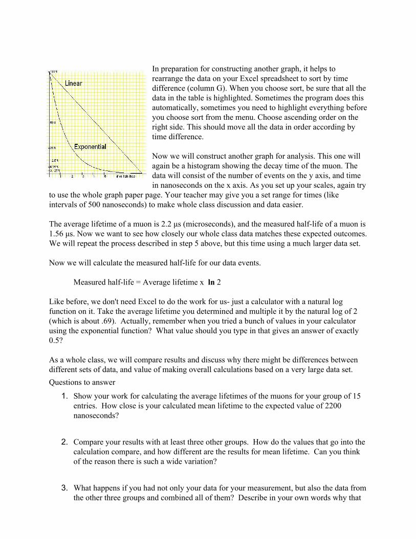
In preparation for constructing another graph, it helps to rearrange the data on your Excel spreadsheet to sort by time difference (column G). When you choose sort, be sure that all the data in the table is highlighted. Sometimes the program does this automatically, sometimes you need to highlight everything before you choose sort from the menu. Choose ascending order on the right side. This should move all the data in order according by time difference. Now we will construct another graph for analysis. This one will again be a histogram showing the decay time of the muon. The data will consist of the number of events on the y axis, and time in nanoseconds on the x axis. As you set up your scales, again try

to use the whole graph paper page. Your teacher may give you a set range for times (like intervals of 500 nanoseconds) to make whole class discussion and data easier. The average lifetime of a muon is 2.2 μs (microseconds), and the measured half­life of a muon is 1.56 μs. Now we want to see how closely our whole class data matches these expected outcomes. We will repeat the process described in step 5 above, but this time using a much larger data set. Now we will calculate the measured half­life for our data events.

Measured half­life = Average lifetime x ln 2

Like before, we don't need Excel to do the work for us­ just a calculator with a natural log function on it. Take the average lifetime you determined and multiple it by the natural log of 2 (which is about .69). Actually, remember when you tried a bunch of values in your calculator using the exponential function? What value should you type in that gives an answer of exactly 0.5? As a whole class, we will compare results and discuss why there might be differences between different sets of data, and value of making overall calculations based on a very large data set. Questions to answer

1. Show your work for calculating the average lifetimes of the muons for your group of 15 entries. How close is your calculated mean lifetime to the expected value of 2200 nanoseconds?

2. Compare your results with at least three other groups. How do the values that go into the calculation compare, and how different are the results for mean lifetime. Can you think of the reason there is such a wide variation?

3. What happens if you had not only your data for your measurement, but also the data from the other three groups and combined all of them? Describe in your own words why that

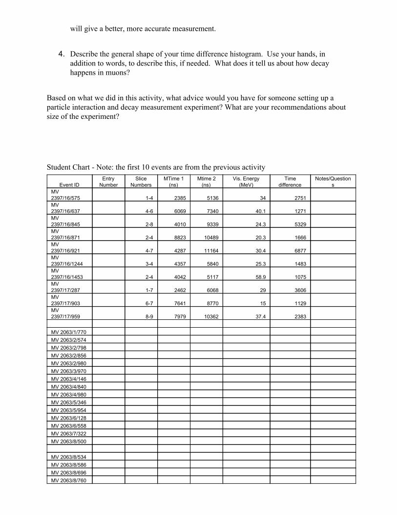
will give a better, more accurate measurement.

4. Describe the general shape of your time difference histogram. Use your hands, in addition to words, to describe this, if needed. What does it tell us about how decay happens in muons?

Based on what we did in this activity, what advice would you have for someone setting up a particle interaction and decay measurement experiment? What are your recommendations about size of the experiment? Student Chart ­ Note: the first 10 events are from the previous activity

Event ID Entry Number

Slice Numbers

MTime 1 (ns)

Mtime 2 (ns)

Vis. Energy (MeV)

Time difference

Notes/Questions

MV 2397/16/575 1­4 2385 5136 34 2751 MV 2397/16/637 4­6 6069 7340 40.1 1271 MV 2397/16/845 2­8 4010 9339 24.3 5329 MV 2397/16/871 2­4 8823 10489 20.3 1666 MV 2397/16/921 4­7 4287 11164 30.4 6877 MV 2397/16/1244 3­4 4357 5840 25.3 1483 MV 2397/16/1453 2­4 4042 5117 58.9 1075 MV 2397/17/287 1­7 2462 6068 29 3606 MV 2397/17/903 6­7 7641 8770 15 1129 MV 2397/17/959 8­9 7979 10362 37.4 2383 MV 2063/1/770 MV 2063/2/574 MV 2063/2/798 MV 2063/2/856 MV 2063/2/980 MV 2063/3/970 MV 2063/4/146 MV 2063/4/840 MV 2063/4/980 MV 2063/5/346 MV 2063/5/954 MV 2063/6/128 MV 2063/6/558 MV 2063/7/322 MV 2063/8/500 MV 2063/8/534 MV 2063/8/586 MV 2063/8/696 MV 2063/8/760

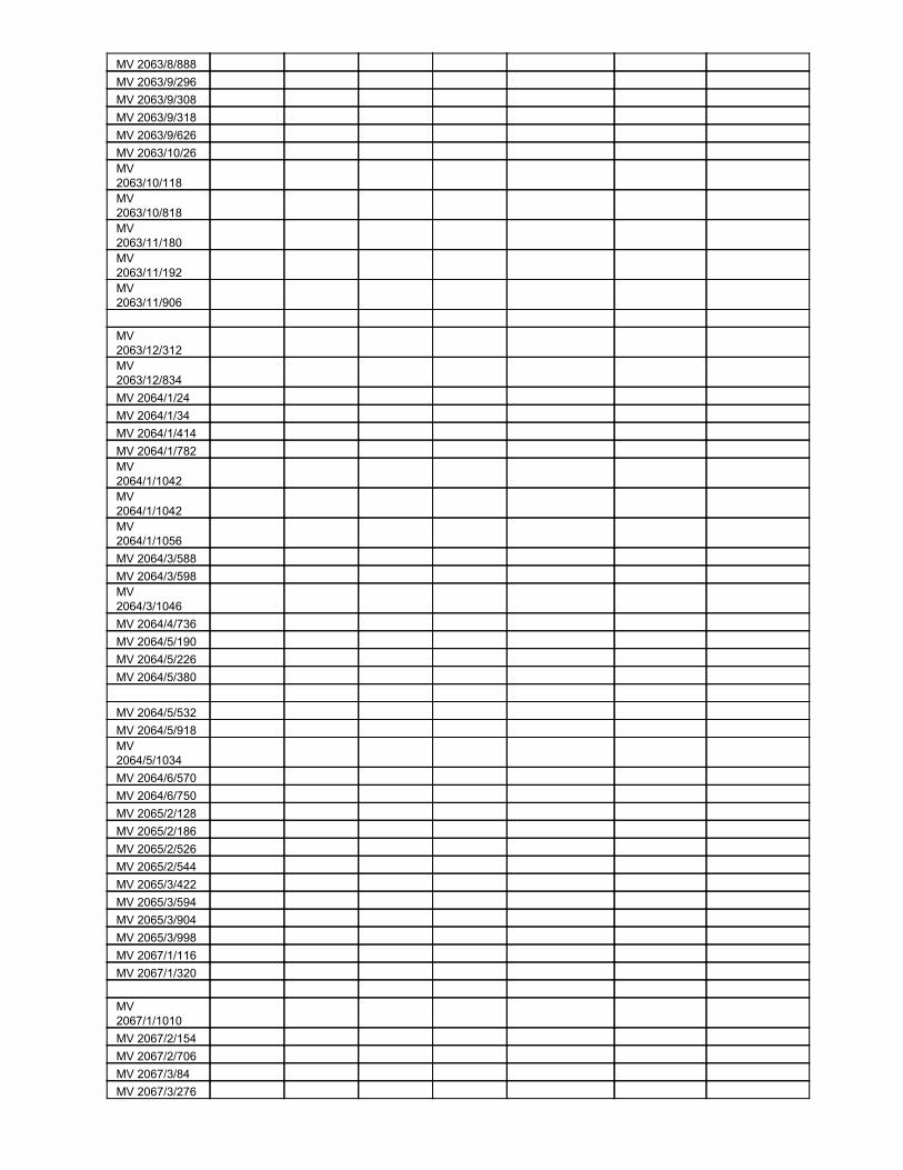
MV 2063/8/888 MV 2063/9/296 MV 2063/9/308 MV 2063/9/318 MV 2063/9/626 MV 2063/10/26 MV 2063/10/118 MV 2063/10/818 MV 2063/11/180 MV 2063/11/192 MV 2063/11/906 MV 2063/12/312 MV 2063/12/834 MV 2064/1/24 MV 2064/1/34 MV 2064/1/414 MV 2064/1/782 MV 2064/1/1042 MV 2064/1/1042 MV 2064/1/1056 MV 2064/3/588 MV 2064/3/598 MV 2064/3/1046 MV 2064/4/736 MV 2064/5/190 MV 2064/5/226 MV 2064/5/380 MV 2064/5/532 MV 2064/5/918 MV 2064/5/1034 MV 2064/6/570 MV 2064/6/750 MV 2065/2/128 MV 2065/2/186 MV 2065/2/526 MV 2065/2/544 MV 2065/3/422 MV 2065/3/594 MV 2065/3/904 MV 2065/3/998 MV 2067/1/116 MV 2067/1/320 MV 2067/1/1010 MV 2067/2/154 MV 2067/2/706 MV 2067/3/84 MV 2067/3/276

MV 2067/4/740 MV 2067/4/1014 MV 2067/4/1108 MV 2067/4/1164 MV 2067/5/108 MV 2067/5/748 MV 2067/6/226 MV 2067/6/606 MV 2067/6/690 MV 2067/6/832 MV 2067/6/1060 MV 2067/7/216 MV 2067/8/788 MV 2067/68/802 MV 2067/8/924 MV 2067/8/976 MV 2067/9/86 MV 2067/9/174 MV 2067/89/220 MV 2067/9/718 MV 20679/760 MV 2067/10/146 MV 2067/10/1048 MV 2067/10/1152 MV 2067/11//90 MV 2067/11/872 MV 2067/11/896 MV 2067/11/896 MV 2067/12/92 MV 2067/12/92 MV 2067/12/322 MV 2067/13/2 MV 2067/13/268 MV 2067/13/448 MV 2067/13/490 MV 2067/13/514 MV 2067/13/826 MV 2067/14/274 MV 2067/14/448 MV 2067/14/522 MV 2067/14/1074

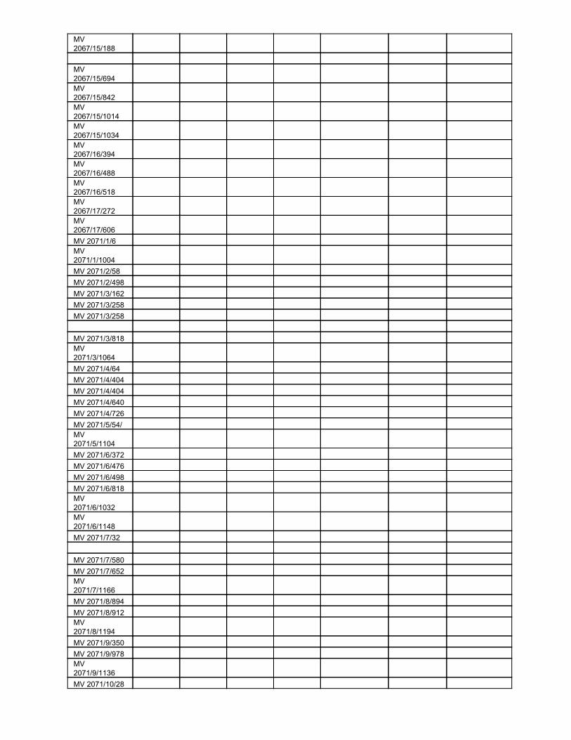
MV 2067/15/188 MV 2067/15/694 MV 2067/15/842 MV 2067/15/1014 MV 2067/15/1034 MV 2067/16/394 MV 2067/16/488 MV 2067/16/518 MV 2067/17/272 MV 2067/17/606 MV 2071/1/6 MV 2071/1/1004 MV 2071/2/58 MV 2071/2/498 MV 2071/3/162 MV 2071/3/258 MV 2071/3/258 MV 2071/3/818 MV 2071/3/1064 MV 2071/4/64 MV 2071/4/404 MV 2071/4/404 MV 2071/4/640 MV 2071/4/726 MV 2071/5/54/ MV 2071/5/1104 MV 2071/6/372 MV 2071/6/476 MV 2071/6/498 MV 2071/6/818 MV 2071/6/1032 MV 2071/6/1148 MV 2071/7/32 MV 2071/7/580 MV 2071/7/652 MV 2071/7/1166 MV 2071/8/894 MV 2071/8/912 MV 2071/8/1194 MV 2071/9/350 MV 2071/9/978 MV 2071/9/1136 MV 2071/10/28

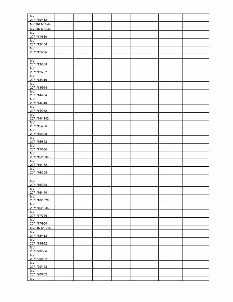
MV 2071/10/412 MV 2071/11/44 MV 2071/11/44 MV 2071/11/810 MV 2071/12/156 MV 2071/12/226 MV 2071/12/268 MV 2071/12/752 MV 2071/13/310 MV 2071/13/948 MV 2071/14/204 MV 2071/14/340 MV 2071/14/942 MV 2071/14/1142 MV 2071/15/766 MV 2071/15/808 MV 2071/15/852 MV 2071/15/884 MV 2071/15/1034 MV 2071/16/172 MV 2071/16/258 MV 2071/16/388 MV 2071/16/440 MV 2071/16/1028 MV 2071/16/1036 MV 2071/17/746 MV 2071/17/950 MV 2071/18/16 MV 2071/18/412 MV 2071/18/952 MV 2071/20/304 MV 2071/20/402 MV 2071/20/458 MV 2071/20/702 MV

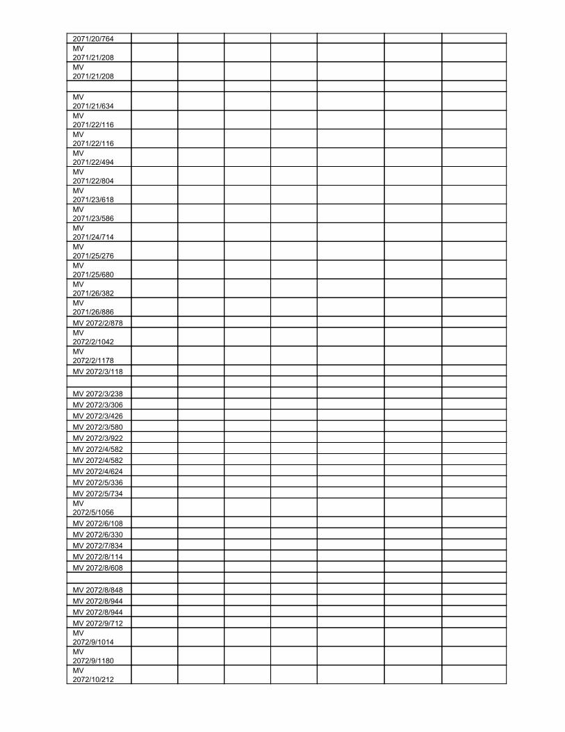
2071/20/764 MV 2071/21/208 MV 2071/21/208 MV 2071/21/634 MV 2071/22/116 MV 2071/22/116 MV 2071/22/494 MV 2071/22/804 MV 2071/23/618 MV 2071/23/586 MV 2071/24/714 MV 2071/25/276 MV 2071/25/680 MV 2071/26/382 MV 2071/26/886 MV 2072/2/878 MV 2072/2/1042 MV 2072/2/1178 MV 2072/3/118 MV 2072/3/238 MV 2072/3/306 MV 2072/3/426 MV 2072/3/580 MV 2072/3/922 MV 2072/4/582 MV 2072/4/582 MV 2072/4/624 MV 2072/5/336 MV 2072/5/734 MV 2072/5/1056 MV 2072/6/108 MV 2072/6/330 MV 2072/7/834 MV 2072/8/114 MV 2072/8/608 MV 2072/8/848 MV 2072/8/944 MV 2072/8/944 MV 2072/9/712 MV 2072/9/1014 MV 2072/9/1180 MV 2072/10/212

MV 2072/10/212 MV 2072/10/572 MV 2072/10/698 MV 2072/11/352 MV 2072/11/416 MV 2072/11/818 MV 2072/11/1020 MV 2072/11/1096 MV 2072/12/224 MV 2072/13/678

Activity: Energy of Decay Electrons (Understanding why the electrons in muon decay have this distribution of energy) This is the suggested fourth activity in the muon radioactive decay lessons.

This is an advanced activity, suitable if you have a lot of time or have one or two students interested in a little more. But it has a compelling and historical detective story. The student instructions lead them and you through the argument through a process of elimination. Here are a few additional notes.

Goals: 1. Apply Einstein’s E=mc2 to understand how much kinetic energy is shared among the

decay products 2. By process of elimination, and conservation of energy and momentum, conclude that

there must be at least two unseen particles along with the electron after the decay.

Prior Knowledge: 1. Conservation of momentum and energy, in the billiard ball sense. 2. That mass is a form of energy, and Einstein says they are related by E=mc2 3. Radioactive decay, from the three activities that precede this one.

Materials: 1. Graph paper to make a histogram 2. The energy data from the spreadsheet in the previous activity 3. The student instructions and questions below.

Notes for the teacher: The arguments that are central to this activity are by themselves simple, but to reach the conclusion requires stringing them together and considering specific consequences of the situation, not just general principles. This is a rewarding challenge, and you may want to allow your students plenty of time to think things through and talk out loud with their partners. As Sherlock Holmes said, “When you have eliminated the impossible, whatever remains, however improbable, must be the truth”. This is one of those situations. Notice in the suggested answers that we are making semi­quantitative arguments. Lots of students have a great resistance to this, but if you hear them stepping toward a correct answer, consider challenging them with the question “what are the consequences of your argument if your electron has this energy” and point somewhere in their histogram. See how they respond.

Answers to the student activity questions: Option one. Suppose that only one particle, the electron, came out. Given the energy available and the kinetic energies in the histogram, do you notice something odd? Thinking about an

electron moving with any of those kinetic energies what do you conclude about conservation of momentum? Answer. The electron must have all 106 MeV of kinetic energy, but clearly that is not what I measured, I usually only saw half of that. And if the electron is the only particle, and it has that much kinetic energy, it must have some momentum, because even if it has 30 MeV, it really is moving, right? But there was no momentum before (muon at rest), so having momentum after would violate a conservation law, which I would never do, officer, really. This situation not only does not describe the electrons I measured, but it's physically impossible. Option two. Suppose that two particles came out: the electron that you can see, and a neutrino or neutrissimo or something which you don’t see. To simplify the argument for a second, enough that you can do the math in your head, pretend these two particles have equal mass, like billiard balls. Consider conservation of momentum, what must be the direction of the neutral particle you didn’t see, relative to the electron you did see? Given the available energy, what must be the kinetic energy of each of these two particles? If that was really how it worked, what would your energy histogram have looked like? [This conclusion stands even if the masses of the two particles are different, it just requires a more difficult calculation to figure out what energy would have been in the.] Answer: This one is tricky, but if I assume both particles have the same mass, it really is easier. In this case, they must come out back to back (so 2D vector momentum sums to zero and is conserved). If that happens, and they have the same mass, then they also have the same momentum and must have equally shared the available energy, and have 53 MeV each. In this case, ALL the electrons should have 53 MeV, they all would be piled up in 50 to 55 MeV interval in the histogram. That’s clearly not what I see. Longer answer: If the masses of the electron and neutrino were different, they would still be piled up in just one interval in the histogram, they would still come out back­to­back, but which one (between 0 and 106) depends on what the two masses are. Mathematically, you set up conservation of energy, conservation of momentum, and get two equations and two unknowns, which has exactly one solution. Option three. Supposed three particles came out. How does this situation change or overcome the issues you wrestled with for the previous two options. Answer: I certainly don’t have the problem I had in option one, I have three particles to share the energy and conserve momentum. The three particles don’t have to come out perfectly back to back anymore; in fact I can imagine all sorts of combinations of directions that still balance momentum. If I give the electron only 20 MeV of energy, then I just give the neutrinos the other 86, and make sure they make a wide enough angle from each other, centered on a line backward from the electron. Change the electron energy higher; make the angle between the two neutrinos smaller. [It is not super clear from this qualitative argument that the limiting case is that the electron can carry at most half the available energy, like the argument in option two, but this is also true.] Summarize as succinctly as you can summarize the process of elimination that leads from your histogram to your conclusion that there must be at least two unseen particles with the electron after the decay. Having only one particle after the decay is impossible; no way can it conserve energy and momentum. Having two particles is possible, but then I would expect a single energy somewhere between zero and 106 MeV, but instead I see a range of energies. Having eliminated the two simplest possibilities, I can imagine that having three particles will work; they give me

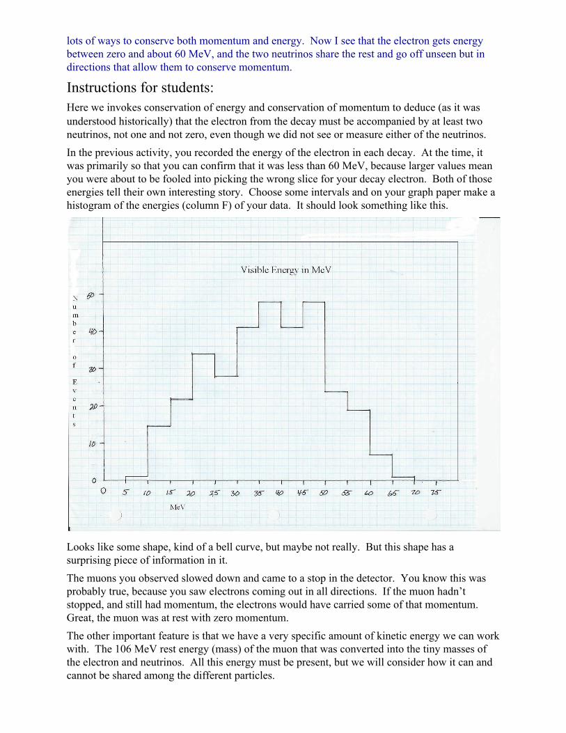
lots of ways to conserve both momentum and energy. Now I see that the electron gets energy between zero and about 60 MeV, and the two neutrinos share the rest and go off unseen but in directions that allow them to conserve momentum.

Instructions for students: Here we invokes conservation of energy and conservation of momentum to deduce (as it was understood historically) that the electron from the decay must be accompanied by at least two neutrinos, not one and not zero, even though we did not see or measure either of the neutrinos. In the previous activity, you recorded the energy of the electron in each decay. At the time, it was primarily so that you can confirm that it was less than 60 MeV, because larger values mean you were about to be fooled into picking the wrong slice for your decay electron. Both of those energies tell their own interesting story. Choose some intervals and on your graph paper make a histogram of the energies (column F) of your data. It should look something like this.

Looks like some shape, kind of a bell curve, but maybe not really. But this shape has a surprising piece of information in it. The muons you observed slowed down and came to a stop in the detector. You know this was probably true, because you saw electrons coming out in all directions. If the muon hadn’t stopped, and still had momentum, the electrons would have carried some of that momentum. Great, the muon was at rest with zero momentum. The other important feature is that we have a very specific amount of kinetic energy we can work with. The 106 MeV rest energy (mass) of the muon that was converted into the tiny masses of the electron and neutrinos. All this energy must be present, but we will consider how it can and cannot be shared among the different particles.

Consider the following options for the decay. Option one. Suppose that only one particle, the electron, came out. Given the energy available and the kinetic energies in the histogram, do you notice something odd? Thinking about an electron moving with any of those kinetic energies what do you conclude about conservation of momentum? Option two. Suppose that two particles came out, the electron which you can see, and a neutrino or something which you don’t see. To simplify the argument for a second, enough that you can do the math in your head, pretend these two particles have equal mass, like billiard balls. Consider conservation of momentum, what must be the direction of the neutral particle you didn’t see, relative to the electron you did see? Given the available energy, what must be the kinetic energy of each of these two particles? If that was really how it worked, what would your energy histogram have looked like? [This conclusion stands even if the masses of the two particles are different, it just requires a more difficult calculation to figure out what energy would have been in the.] Option three. Supposed three particles came out. How does this situation change or overcome the issues you wrestled with for the previous two options. Summarize as succinctly as you can summarize the process of elimination that leads from your histogram to your conclusion that there must be at least two unseen particles with the electron after the decay.

Quiz: ‘What is MINERvA’? Goal: This quick quiz is meant to be used after viewing the What is MINERvA? ­ PowerPoint (found in the activities section of the website). The quiz is located at the end of the presentation but is given here in case the teacher would prefer a printed copy.

Quiz MINERvA

(Main INjector ExpeRiment) for v­A

1. What does the MINERvA detector measure?

2. What shape is each of the planes in MINERvA?

3. What is a scintillator strip?

4. What is the shape of a scintillator strip?

5. How many specialized areas are in MINERvA?

6. Name 3 types of material in MINERvA.

7. What is a wavelength shifting fiber?

8. What does a PMT do?

ANSWER KEY

1. What does the MINERvA detector measure? It measures low energy neutrino interactions (interactions of protons,

muons and pions in particular) 2. What shape is each of the planes in MINERvA?

Each plane is in the shape of a hexagon. 3. What is a scintillator strip?

It is a material that takes the energy from an interacting particle and turns it into light. 4. What is the shape of a scintillator strip?

Triangular shaped and come in long strips.

5. How many specialized areas are in MINERvA? There are three areas: The fully active target, the ECAL and the

HCAL. 6. Name 3 types of material in MINERvA.

Currently the detector has specialized areas made out of hydrocarbon, carbon, iron and lead. There are plans to add helium and water targets in the near future. 7. What is a wavelength shifting fiber?

It takes the light and collects it and sends it to the PMT’s. (It also shifts the wavelength of the light to better collect it.) 8. What does a PMT do?

The signal from the detector will be a very weak signal. The computers are not able to read neither the minute strength of the signal nor do they recognize the photons that they are receiving from the detector. The PMT takes the photons and amplifies the signal. It also transfers the signal into a form of energy which is more easily understood by the computers.

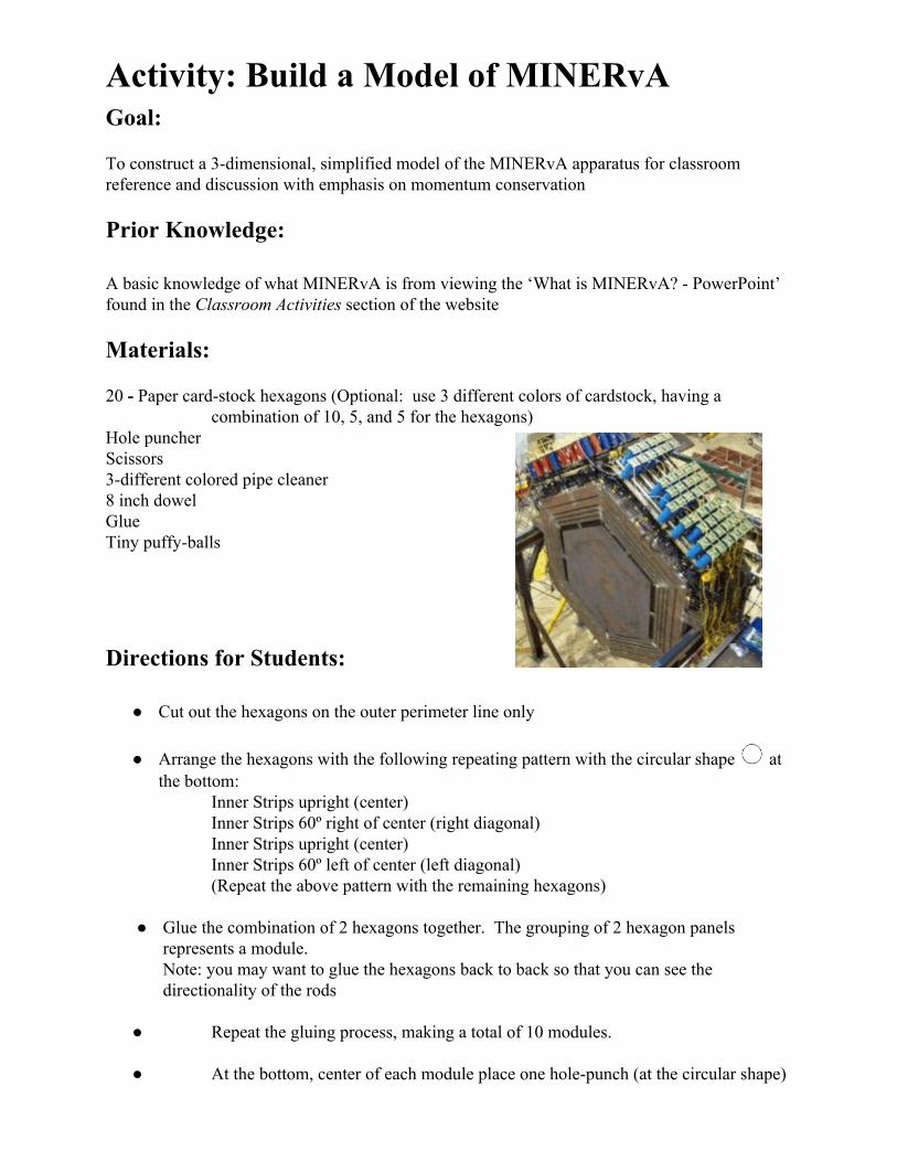
Activity: Build a Model of MINERvA Goal: To construct a 3­dimensional, simplified model of the MINERvA apparatus for classroom reference and discussion with emphasis on momentum conservation Prior Knowledge: A basic knowledge of what MINERvA is from viewing the ‘What is MINERvA? ­ PowerPoint’ found in the Classroom Activities section of the website Materials: 20 ­ Paper card­stock hexagons (Optional: use 3 different colors of cardstock, having a

combination of 10, 5, and 5 for the hexagons) Hole puncher Scissors 3­different colored pipe cleaner 8 inch dowel Glue Tiny puffy­balls

Directions for Students:

Cut out the hexagons on the outer perimeter line only Arrange the hexagons with the following repeating pattern with the circular shape at

the bottom: Inner Strips upright (center) Inner Strips 60º right of center (right diagonal) Inner Strips upright (center) Inner Strips 60º left of center (left diagonal) (Repeat the above pattern with the remaining hexagons)

Glue the combination of 2 hexagons together. The grouping of 2 hexagon panels

represents a module. Note: you may want to glue the hexagons back to back so that you can see the directionality of the rods

Repeat the gluing process, making a total of 10 modules.

At the bottom, center of each module place one hole­punch (at the circular shape)

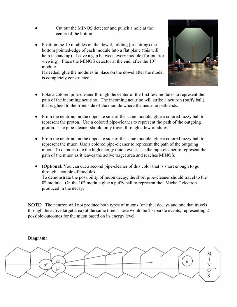
Cut out the MINOS detector and punch a hole at the center of the bottom

Position the 10 modules on the dowel, folding (or cutting) the

bottom pointed­edge of each module into a flat plane (this will help it stand up). Leave a gap between every module (for interior viewing). Place the MINOS detector at the end, after the 10th module. If needed, glue the modules in place on the dowel after the model is completely constructed.

Poke a colored pipe­cleaner through the center of the first few modules to represent the path of the incoming neutrino. The incoming neutrino will strike a neutron (puffy ball) that is glued to the front side of the module where the neutrino path ends.

From the neutron, on the opposite side of the same module, glue a colored fuzzy ball to

represent the proton. Use a colored pipe­cleaner to represent the path of the outgoing proton. The pipe­cleaner should only travel through a few modules

From the neutron, on the opposite side of the same module, glue a colored fuzzy ball to

represent the muon. Use a colored pipe­cleaner to represent the path of the outgoing muon. To demonstrate the high energy muon event, use the pipe­cleaner to represent the path of the muon as it leaves the active target area and reaches MINOS.

(Optional: You can cut a second pipe­cleaner of this color that is short enough to go

through a couple of modules. To demonstrate the possibility of muon decay, the short pipe­cleaner should travel to the 8th module. On the 10th module glue a puffy ball to represent the “Michel” electron produced in the decay.

NOTE: The neutron will not produce both types of muons (one that decays and one that travels through the active target area) at the same time. These would be 2 separate events; representing 2 possible outcomes for the muon based on its energy level. Diagram:

Analysis Questions:

1. Write the reaction for a neutrino striking a neutron:

2. Explain the significance of each module consisting of 2 panels in different planes? __________________________________________________________________

__________________________________________________________________ __________________________________________________________________ __________________________________________________________________

3. What is the purpose of the MINOS detector at the end the MINERvA experiment? ____________________________________________________________________

____________________________________________________________________ ____________________________________________________________________ ____________________________________________________________________

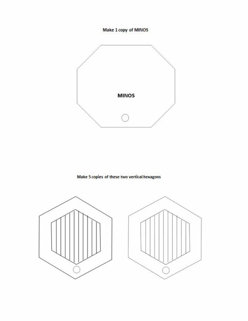
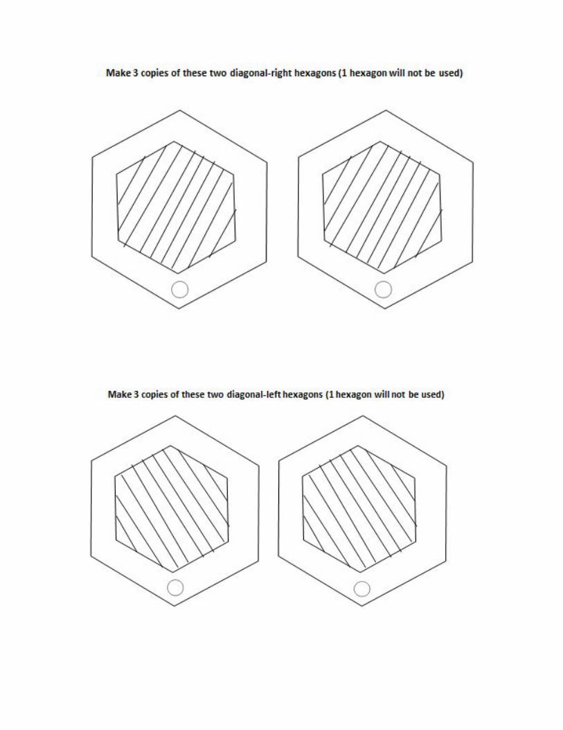
Activity: Conservation of Momentum when Neutrinos Interact This teacher­guided activity is the first suggested activity in learning about scattering of neutrinos and applying conservation of momentum. Goal:

In this teacher­guided activity, students will be introduced to the concept of conservation of momentum and energy at the particle level. Teacher Background: Before starting this activity, students should have already gone through the ‘Directions for the Simple Arachne Website’ since they will have a have a level of comfort within the website and the information they need to record about the interaction. Another resource to view prior to this activity is the ‘Bug and Truck Collision’ PowerPoint (found on the main website, “Momentum conservation” page and under the “Activities and Resources"). The PowerPoint provides a humorous visual representation of the collision and its products. To access the data, be sure that the student computers have Firefox installed for internet usage. The Arachne website will not work on Internet Explorer After reviewing the Student Background information with the class, teachers will guide the students through several examples of collisions. Have the students open the first collision. Guide them to highlight either the shorter or longer track. The longer track will be the path of the muon and the shorter track will be the path of the heavier proton. When they hold the cursor over one of the tracks the color will change to red. A drop­down box will appear. Make sure they choose the correct particle information for the path they have selected and record it on their collection sheet. (You will also notice the ‘Copy’ box. If you prefer, students can have the information copied and pasted into an excel file instead of using the Collection sheet provided) Repeat the same procedure for the other path. It is very important that they write down the negative sign if it appears next to the momentum values. If you choose you can guide the students through the first few events and then let them try the remainder in small groups. After the students have recorded data from 10 events, the sum of the values should be calculated. Students will find that the sum of the px and the sum of the py do not equal zero. This will lend itself to the discussion of ‘Is the neutron at rest inside the nucleus?’ You may want to refer back to the ‘Bug and Truck Collision’ PowerPoint for visual explanation.

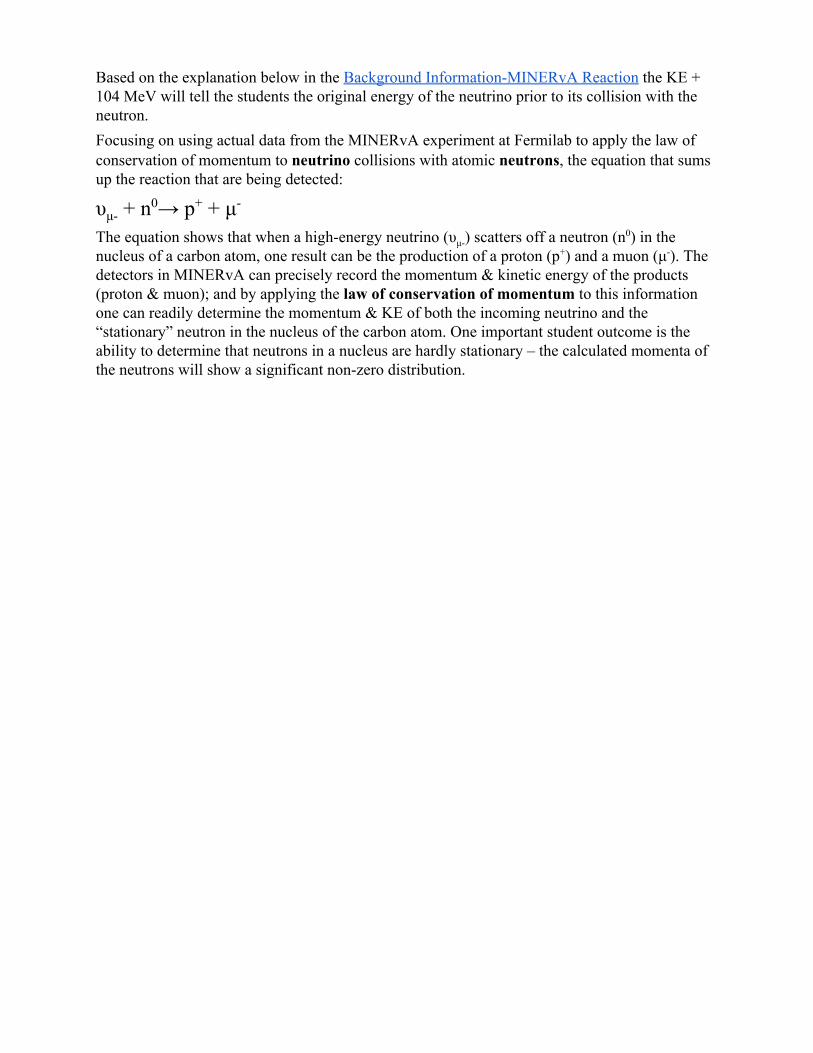
Based on the explanation below in the Background Information­MINERvA Reaction the KE + 104 MeV will tell the students the original energy of the neutrino prior to its collision with the neutron. Focusing on using actual data from the MINERvA experiment at Fermilab to apply the law of conservation of momentum to neutrino collisions with atomic neutrons, the equation that sums up the reaction that are being detected:

υμ­ + n0→ p+ + μ­ The equation shows that when a high­energy neutrino (υμ­) scatters off a neutron (n0) in the nucleus of a carbon atom, one result can be the production of a proton (p+) and a muon (μ­). The detectors in MINERvA can precisely record the momentum & kinetic energy of the products (proton & muon); and by applying the law of conservation of momentum to this information one can readily determine the momentum & KE of both the incoming neutrino and the “stationary” neutron in the nucleus of the carbon atom. One important student outcome is the ability to determine that neutrons in a nucleus are hardly stationary – the calculated momenta of the neutrons will show a significant non­zero distribution.

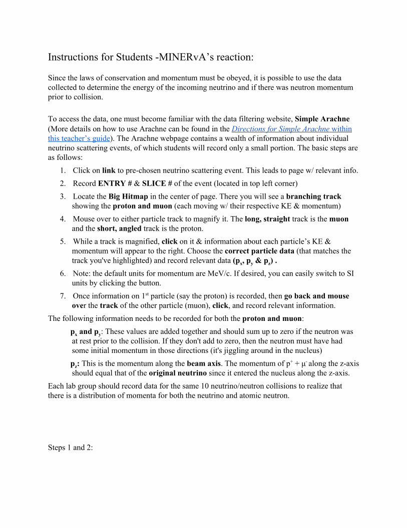
Instructions for Students ­MINERvA’s reaction: Since the laws of conservation and momentum must be obeyed, it is possible to use the data collected to determine the energy of the incoming neutrino and if there was neutron momentum prior to collision.

To access the data, one must become familiar with the data filtering website, Simple Arachne (More details on how to use Arachne can be found in the Directions for Simple Arachne within this teacher’s guide). The Arachne webpage contains a wealth of information about individual neutrino scattering events, of which students will record only a small portion. The basic steps are as follows:

1. Click on link to pre­chosen neutrino scattering event. This leads to page w/ relevant info. 2. Record ENTRY # & SLICE # of the event (located in top left corner) 3. Locate the Big Hitmap in the center of page. There you will see a branching track

showing the proton and muon (each moving w/ their respective KE & momentum) 4. Mouse over to either particle track to magnify it. The long, straight track is the muon

and the short, angled track is the proton. 5. While a track is magnified, click on it & information about each particle’s KE &

momentum will appear to the right. Choose the correct particle data (that matches the track you've highlighted) and record relevant data (px, py & pz) .

6. Note: the default units for momentum are MeV/c. If desired, you can easily switch to SI units by clicking the button.

7. Once information on 1st particle (say the proton) is recorded, then go back and mouse over the track of the other particle (muon), click, and record relevant information.

The following information needs to be recorded for both the proton and muon: px and py: These values are added together and should sum up to zero if the neutron was

at rest prior to the collision. If they don't add to zero, then the neutron must have had some initial momentum in those directions (it's jiggling around in the nucleus)

pz: This is the momentum along the beam axis. The momentum of p+ + μ­ along the z­axis should equal that of the original neutrino since it entered the nucleus along the z­axis.

Each lab group should record data for the same 10 neutrino/neutron collisions to realize that there is a distribution of momenta for both the neutrino and atomic neutron. Steps 1 and 2:

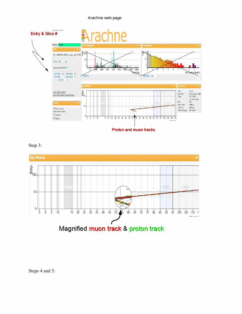
Step 3:

Steps 4 and 5:

Step 7:

Conservation of Momentum Events Events are posted at http://neutrino­classroom.org/momentum_conservation.html#collisions in groups of 20 per group. Note: Arachne requires a recent version of a web browser, such as Firefox version 4.0, Safari version 4.0, and Chrome version 5.0. Arachne relies on Java and parts of the HTML5 standard to more dynamically render the images and make them interactive. Because it does not yet support the latter, the Internet Explorer browser will not run Arachne.

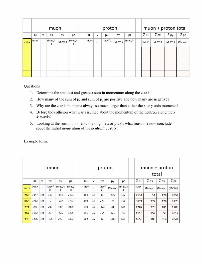
muon

proton

muon + proton total KE v px py pz KE v px py pz ΣKE Σpx Σpy Σpz

entry (MeV) c (MeV/c

) (MeV/c) (MeV/c)

(MeV) c (MeV/c

) (MeV/c) (MeV/c) (MeV) (MeV/c) (MeV/c) (MeV/c)

Questions

1. Determine the smallest and greatest sum in momentum along the z­axis. 2. How many of the sum of px and sum of py are positive and how many are negative? 3. Why are the z­axis momenta always so much larger than either the x or y­axis momenta? 4. Before the collision what was assumed about the momentum of the neutron along the x

& y­axis? 5. Looking at the sum in momentum along the x & y­axis what must one now conclude

about the initial momentum of the neutron? Justify. Example form:

muon

proton

muon + proton total

KE v px py pz KE v px py pz ΣKE Σpx Σpy Σpz

entry (MeV)

c (MeV/c)

(MeV/c)

(MeV/c)

(MeV)

c (MeV/c)

(MeV/c) (MeV/c)

(MeV) (MeV/c) (MeV/c) (MeV/c)

268 7347 1.0 340 -394 7433 184 0.5 -394 216 422 7531 54 178 7854

866 3712 1.0 -7 -502 3783 159 0.5 279 74 490 3871 272 428 4273

271 998 1.0 200 149 1069 290 0.6 -473 31 635 1287 273 181 1703

362 1162 1.0 -207 -225 1225 351 0.7 364 171 787 1513 157 55 2012

338 1296 1.0 -135 273 1363 362 0.7 32 -587 681 1658 103 314 2044

Activity: Neutrino Scattering and the Target Nucleus

In this self­guided activity, students will analyze more neutrino interactions using conservation of momentum, and will infer properties of the target neutron inside a carbon nucleus.

Teacher’s Guide: MINERvA Billiard Ball Reaction

Intermediate Level Goals:

Each student or student group uses Arachne to compile data from their own 10 billiard ball type events.

Conservation rules are applied to the compiled data to make determinations about neutrino and neutron momenta for each event.

The results from each student set are merged together to make one “super” set of class data.

The class data set is used to lead students through a discussion about the range of possibilities in these billiard ball reactions. Specifically, there is a range of neutrino momenta that cause the billiard ball type of reaction and there is a range of neutron momenta that reveals something about the motion of a neutron within the nucleus of a carbon atom (the MINERvA experiment uses carbon atoms as the neutron target/source).

Notes of the Teacher

This activity asks your students to use conservation of momentum to investigate a two particle collision between a fast moving neutrino (υμ­) and a “stationary” neutron (n0). Stationary is in quotes because neutrons actually vibrate and zip around the confines of an atom’s nucleus at surprisingly high speeds. A proton and a muon are the particles produced in this collision. The particle collision is represented below: υμ­ + n0→ p+ + μ­

MINERA provides information about each product particles momentum and energy. Students will focus on the product momenta data to:

1. determine the z­axis momentum of the incoming neutrino and, 2. to find the neutron’s x­axis and y­axis velocity within the nucleus at the moment of

collision. This intermediate activity adds a layer of complexity to data analysis because separate student results must be merged together and then presented to the class. Merging can be done by hand with students in the classroom or by the teacher merging student Excel files.

Prerequisite Knowledge: The teacher (and students) must be familiar with Arachne (Instructions here) The teacher (and students) must know the conservation of momentum principles that

apply to this billiard ball type reaction. (See “activities and resources” on Momentum Conservation page)

The teacher must know how to construct histograms from large data sets. (see Teacher background Information for Introducing Histograms to Students)

Incorporating Excel: This activity gives you the option to let your students use Excel to organize, manipulate and display data. The Arachne site is compatible with Excel. Instead of students writing down muon and proton data on a worksheet and then adding the data and graphing it by hand, the computer quickly transfers event data from Arachne to Excel with the click of a few buttons. Then, the students can use Excel formulas to add the data.

When students are comfortable determining if the track information describes the muon or the proton, the next step is to COPY the information into Excel. This is done in three steps

1. clicking on the copy button under Track Information in Arachne (see above), 2. opening an Excel window, and 3. use the PASTE command to put the information into the proper place on an Excel

spreadsheet. An Excel template is provided on the website under the resources for the momentum conservation exercise. This template is useful because it gives a uniform data collection sheet for all students. When students open this template they will see a screen that looks like the screen shot below. Before a student copies data from Arachne into Excel, the entry file number that appears on the left hand side of the Arachne screen should be typed into Excel’s cell A3 under the heading “event”.

Students should copy data from their first Arachne entry file into row 3. Specifically, muon data is pasted into cells B3 through F3. Proton data is pasted into cells H3 through L3. The paste command works if students click on cell B3 for muon data and cell H3 for proton data. For the second Arachne entry file, data is pasted into cells B4 and H4. Data from the third Arachne entry file is pasted into cells B5 and H5, etc. Muon and proton data from the 10th Arachne entry file appear in row 12. At this point, it is wise to save a file using a naming system that the teacher has worked out

with students. The naming system will be important when it comes time for the teacher to merge the files into one big “super” Excel spreadsheet.

After students copy data from 10 entries into Excel, Excel will be used to add the energies

and momenta. The space on the template to do this is under columns N through Q. Students must type commands so that Excel sums muon and proton kinetic energies (KE) from a single entry. The momentum, axis by axis. Students must click on cell N3 and type the following command into this cell: =B3+H3 and then press enter.

As the students type, the command will appear in Excel’s cell N3 and look like the snapshot below.

Cell N3 is now populated by the sum of the KE’s that appear in cells B3 and H3 ­­­­­­­­­­­­­­­­­­­­­­­­­­­­­­­­­­­­­­­­­­­­­­­­­­­­­­­­­­­­­­­­­­­­­­­­­­­­­­­­­­­­­­­­­­­­­­­­­­­­­­­­­­­­­­­­­­­­

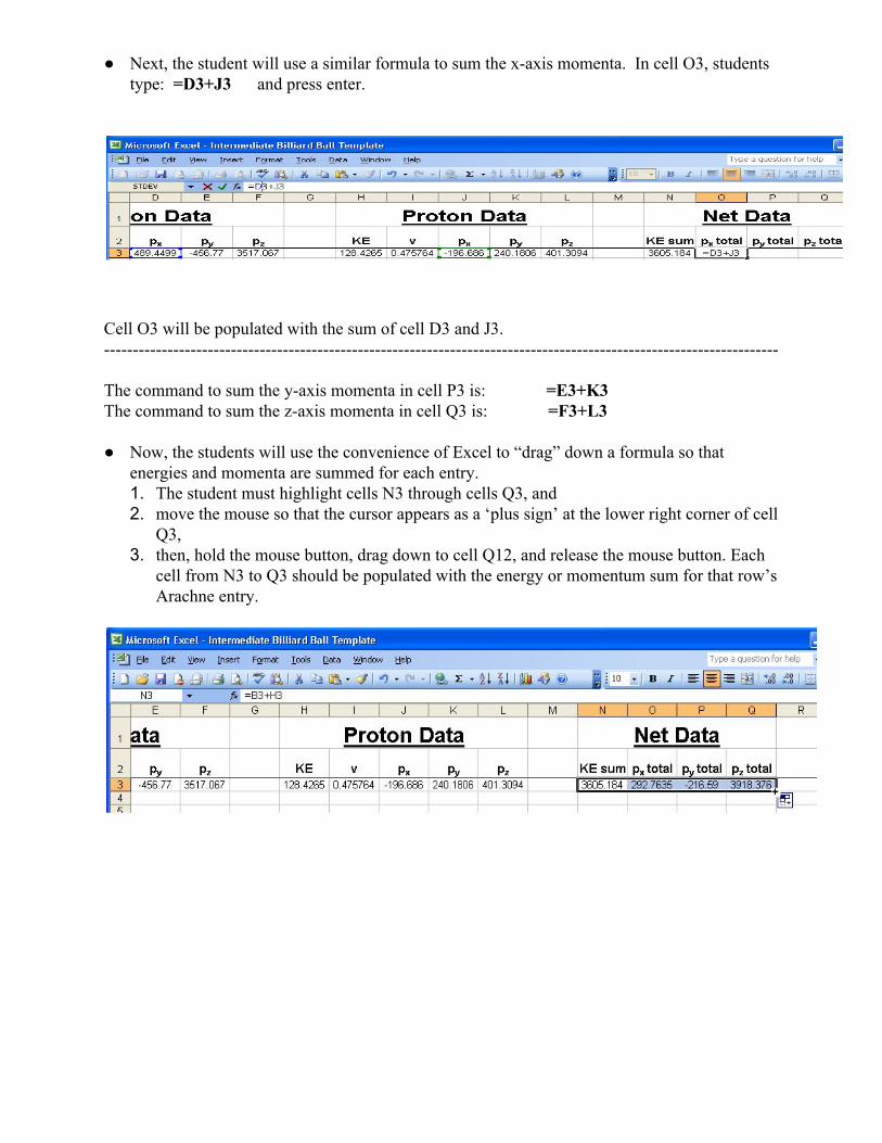
Next, the student will use a similar formula to sum the x­axis momenta. In cell O3, students type: =D3+J3 and press enter.

Cell O3 will be populated with the sum of cell D3 and J3. ­­­­­­­­­­­­­­­­­­­­­­­­­­­­­­­­­­­­­­­­­­­­­­­­­­­­­­­­­­­­­­­­­­­­­­­­­­­­­­­­­­­­­­­­­­­­­­­­­­­­­­­­­­­­­­­­­­­­­ The command to sum the y­axis momenta in cell P3 is: =E3+K3 The command to sum the z­axis momenta in cell Q3 is: =F3+L3 Now, the students will use the convenience of Excel to “drag” down a formula so that

energies and momenta are summed for each entry. 1. The student must highlight cells N3 through cells Q3, and 2. move the mouse so that the cursor appears as a ‘plus sign’ at the lower right corner of cell

Q3, 3. then, hold the mouse button, drag down to cell Q12, and release the mouse button. Each

cell from N3 to Q3 should be populated with the energy or momentum sum for that row’s Arachne entry.

Student data runs for analysis: Use the list of entries your teacher has assigned for your group from the web page with all the sets of links. List of entries (grouped A through T) are found on the web page under the Momentum Conservation tab: Analyzing Neutrino Collisions

Merging Data: After students have completed their Excel template, the data can be merged using the ‘Merging Excel Spreadsheets from Student Groups’ section of this Teacher Guide

Standard Model Poster Scavenger Hunt Goals A fun activity that uses a ‘Standard Model of Fundamental Particle and Interactions’ chart that sends students looking around for the answers. This chart can be found on the internet and in many classrooms Your will need these materials

1. a copy of the Standard Model Chart (found on the Internet or you can make copies of the chart for your classroom

2. Worksheet of questions Notes for Teachers

This activity is designed to be a quick ‘prior­knowledge activity’ so that students become familiar with the vocabulary associated with particle physics Student Instructions and activity sheet

Standard Model Scavenger Hunt – Using a Standard Model of Fundamental particle and Interactions chart, complete the following questions: 1. What is the rest mass of νe?

2. What is the rest mass of a π+?

3. What are the decay particles of a neutron (feel free to draw a picture)?

4. Are neutrinos massless?

5. What are the three fundamental force carriers (bosons) of the fundamental forces?

6. The unit GeV is used energy, GeV is a unit for mass, from what equation are the units based?

7. Rank the leptons in order from least to greatest mass?

8. What is the neutrino oscillation? (Found if using an actual chart. Internet copies do not have the back information)

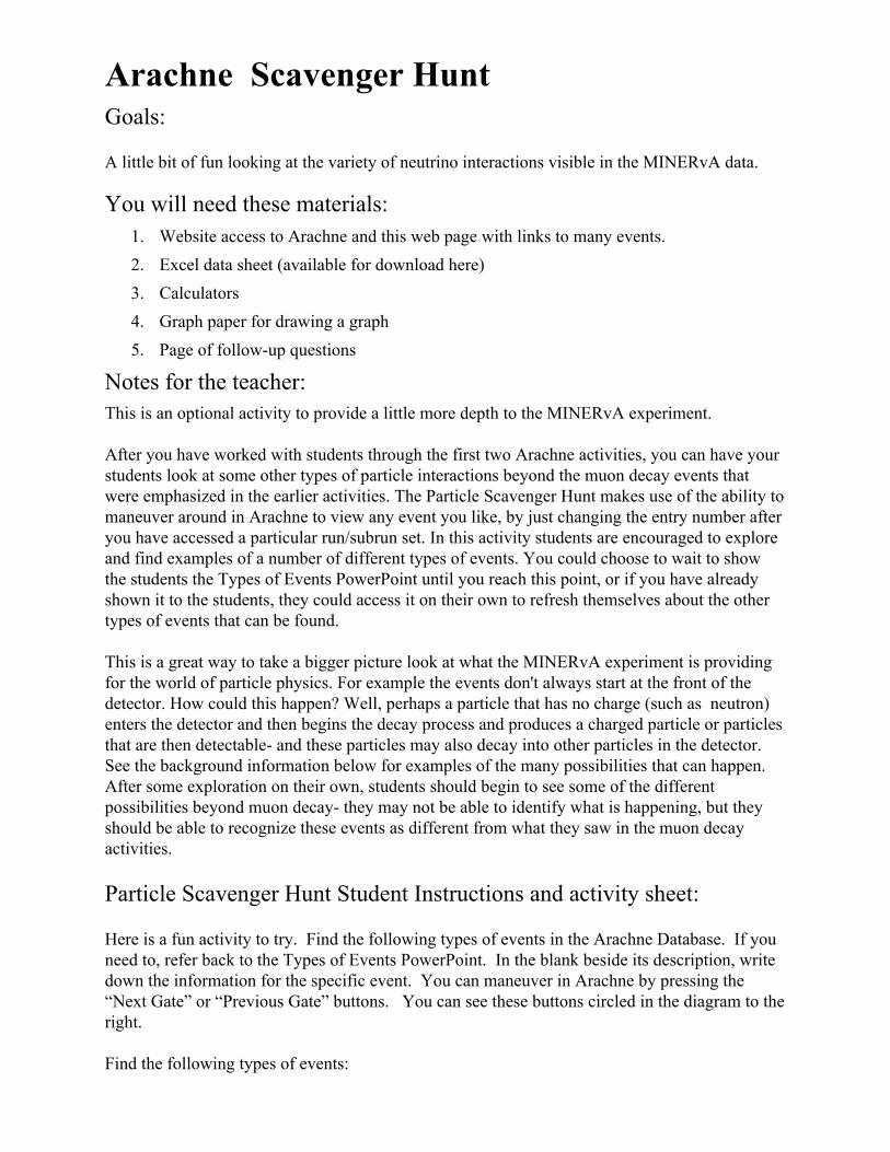
Arachne Scavenger Hunt Goals: A little bit of fun looking at the variety of neutrino interactions visible in the MINERvA data.

You will need these materials: 1. Website access to Arachne and this web page with links to many events. 2. Excel data sheet (available for download here) 3. Calculators 4. Graph paper for drawing a graph 5. Page of follow­up questions

Notes for the teacher: This is an optional activity to provide a little more depth to the MINERvA experiment. After you have worked with students through the first two Arachne activities, you can have your students look at some other types of particle interactions beyond the muon decay events that were emphasized in the earlier activities. The Particle Scavenger Hunt makes use of the ability to maneuver around in Arachne to view any event you like, by just changing the entry number after you have accessed a particular run/subrun set. In this activity students are encouraged to explore and find examples of a number of different types of events. You could choose to wait to show the students the Types of Events PowerPoint until you reach this point, or if you have already shown it to the students, they could access it on their own to refresh themselves about the other types of events that can be found. This is a great way to take a bigger picture look at what the MINERvA experiment is providing for the world of particle physics. For example the events don't always start at the front of the detector. How could this happen? Well, perhaps a particle that has no charge (such as neutron) enters the detector and then begins the decay process and produces a charged particle or particles that are then detectable­ and these particles may also decay into other particles in the detector. See the background information below for examples of the many possibilities that can happen. After some exploration on their own, students should begin to see some of the different possibilities beyond muon decay­ they may not be able to identify what is happening, but they should be able to recognize these events as different from what they saw in the muon decay activities. Particle Scavenger Hunt Student Instructions and activity sheet: Here is a fun activity to try. Find the following types of events in the Arachne Database. If you need to, refer back to the Types of Events PowerPoint. In the blank beside its description, write down the information for the specific event. You can maneuver in Arachne by pressing the “Next Gate” or “Previous Gate” buttons. You can see these buttons circled in the diagram to the right. Find the following types of events:

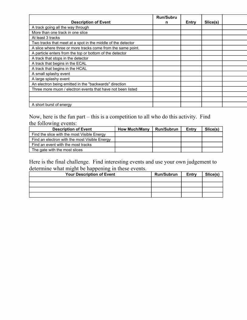
Description of Event Run/Subru

n Entry Slice(s) A track going all the way through More than one track in one slice At least 3 tracks Two tracks that meet at a spot in the middle of the detector A slice where three or more tracks come from the same point. A particle enters from the top or bottom of the detector A track that stops in the detector A track that begins in the ECAL A track that begins in the HCAL A small splashy event A large splashy event An electron being emitted in the "backwards" direction Three more muon / electron events that have not been listed A short burst of energy Now, here is the fun part – this is a competition to all who do this activity. Find the following events:

Description of Event How Much/Many Run/Subrun Entry Slice(s) Find the slice with the most Visible Energy Find an electron with the most Visible Energy Find an event with the most tracks The gate with the most slices Here is the final challenge. Find interesting events and use your own judgement to determine what might be happening in these events.

Your Description of Event Run/Subrun Entry Slice(s)

Additional background information The following information may be useful in your understanding of particle physics. It discusses a few issues that are reasonable questions that you or the students may have, but are not actually needed for doing the activities. Creating a neutrino beam: how do they do it at Fermilab and why does it work? Rules govern particle decay and particle collisions (interactions), each of which are or are related to a conservation law, and require equal amounts of something to be present on both sides of a reaction equation. All of these rules must be followed in every decay/interaction! The examples below are primarily reactions that produce neutrinos or govern neutrino interactions in MINERvA, but you will see or remember the rules applied to muon decay as well.

Charge must be conserved ­­ equal on both sides. For example if the net charge on the left is negative one, there must also be a net charge of negative one on the right side.

Flavors must be conserved­ if there is a representative from the muon family on one side there must also be a muon flavor member of the other side. This can take the form of muon one side and muon neutrino on the other side.

When counting how many muon­flavors there are, a muon has +1 but an anti­muon has ­1. In effect, if you have a muon and an anti­muon­neutrino on the same side you have (+1) + (­1) = 0 muon flavor total. Same with electron flavor and you’ll remember muon decay has an electron and an anti­electron neutrino on one side, for zero total electron flavor.

The number of nucleons (protons or neutrons, doesn’t matter what mixture) on one side must have a corresponding equal number of nucleons on the other side. If there are a proton and a neutron on one side, there must be two nucleons on the other side, often which ones is determined along with the need to conserve charge.

Most importantly, energy and momentum must be conserved. But, totally cool, you can see Einstein's relativity expression E=mc2 in play in these reactions, we can turn mass into energy and vice versa!

So how do you take those rules and use them to get a beam of muon neutrinos for the MINOS and MINERvA experiments? Well, it takes some very large scale stuff to make these incredibly small particles. Start with hydrogen gas, carrying one proton and one electron, right? Strip off the electron, and you have basically just a positively charged proton running around. Speed it all up along with a bazillion other protons to almost the speed of light, and then slam the protons into a carbon target where they hit protons or neutrons of carbon atoms. At this point if a proton hits another proton the result will be a positive pion and a proton and a neutron. If a proton hits a neutron instead you will get either a positive or negative pion and two protons or two neutrons. Possibilities sketched out below.

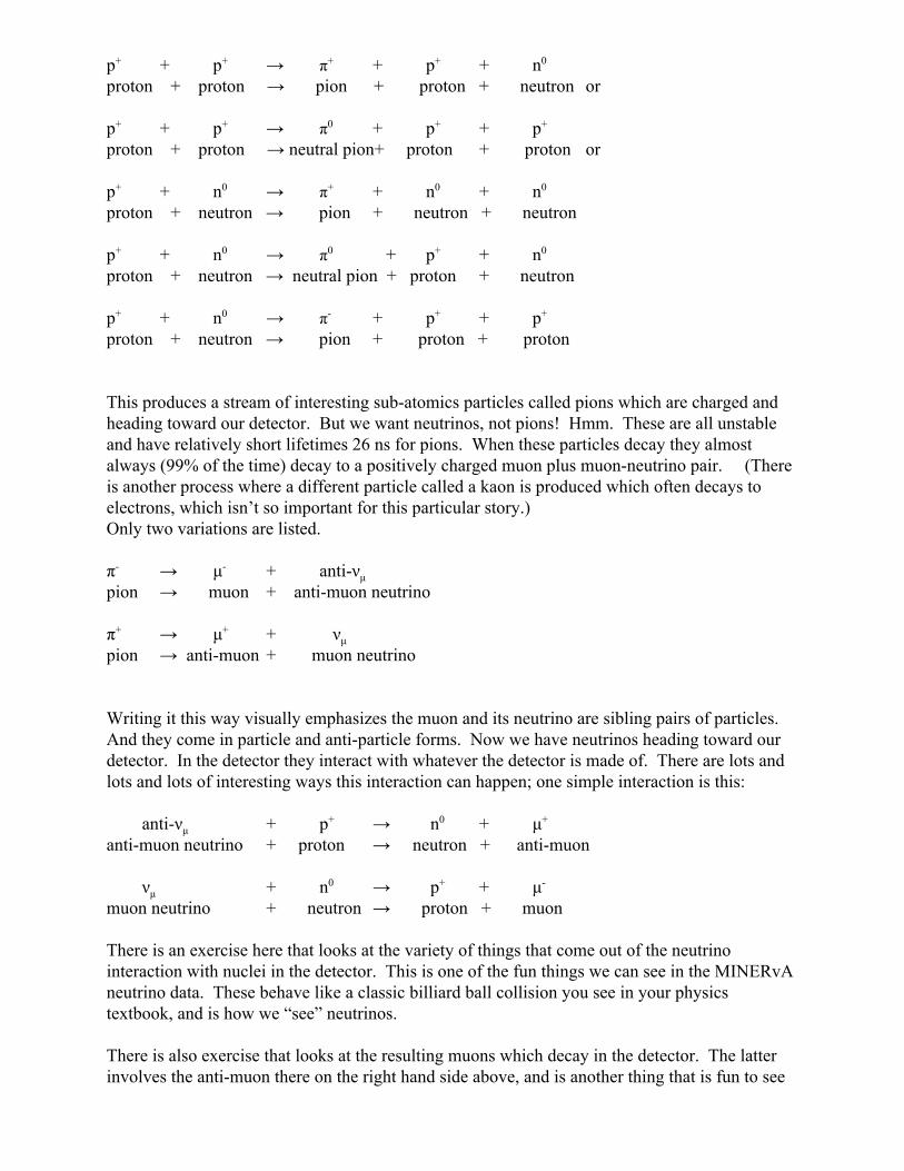
p+ + p+ → π+ + p+ + n0 proton + proton → pion + proton + neutron or p+ + p+ → π0 + p+ + p+ proton + proton → neutral pion+ proton + proton or p+ + n0 → π+ + n0 + n0 proton + neutron → pion + neutron + neutron p+ + n0 → π0 + p+ + n0 proton + neutron → neutral pion + proton + neutron p+ + n0 → π­ + p+ + p+ proton + neutron → pion + proton + proton This produces a stream of interesting sub­atomics particles called pions which are charged and heading toward our detector. But we want neutrinos, not pions! Hmm. These are all unstable and have relatively short lifetimes 26 ns for pions. When these particles decay they almost always (99% of the time) decay to a positively charged muon plus muon­neutrino pair. (There is another process where a different particle called a kaon is produced which often decays to electrons, which isn’t so important for this particular story.) Only two variations are listed. π­ → μ­ + anti­νμ

pion → muon + anti­muon neutrino π+ → μ+ + νμ

pion → anti­muon + muon neutrino Writing it this way visually emphasizes the muon and its neutrino are sibling pairs of particles. And they come in particle and anti­particle forms. Now we have neutrinos heading toward our detector. In the detector they interact with whatever the detector is made of. There are lots and lots and lots of interesting ways this interaction can happen; one simple interaction is this:

anti­νμ + p+ → n0 + μ+

anti­muon neutrino + proton → neutron + anti­muon

νμ + n0 → p+ + μ­

muon neutrino + neutron → proton + muon

There is an exercise here that looks at the variety of things that come out of the neutrino interaction with nuclei in the detector. This is one of the fun things we can see in the MINERvA neutrino data. These behave like a classic billiard ball collision you see in your physics textbook, and is how we “see” neutrinos.

There is also exercise that looks at the resulting muons which decay in the detector. The latter involves the anti­muon there on the right hand side above, and is another thing that is fun to see

in the MINERvA data.

The anti­muon is fun to look at, because unlike the above, we can watch this one decay using the MINERvA detector. Its decay is like this.

μ+ → e+ + νe + anti­νμ anti­muon → positron + electron neutrino + anti­muon neutrino

Wow! We will only be able to see the positron, and interesting, even more neutrinos!

(If you are interested, you notice we followed the negative pion to the anti­muon neutrino to an anti­muon to a positron. Not fully shown here, we can follow the positive pion to the muon neutrino to the negatively charged muon to a negative electron. This is fun too, but negative muons don’t always decay, sometimes they are captured by an atom almost as if they were an electron. But then they often get sucked into the nucleus before they decay, so that’s why we’re not going to concentrate on those.)

.

Merging Excel Spreadsheets from Student Groups Open Excel Sheets to Merge ­ First open Excel. Open the spreadsheets that have the same headers. Now you want to put all of this information in the same spreadsheet. Create a new spreadsheet by clicking the 'new' icon at the top. Merge the Separate Spreadsheets ­ Now go up to 'data' and choose 'consolidate.' A window will open. Choose 'sum' as the function under the drop down menu. Now for the references, click the 'browse' button. Go up to window and choose your first spreadsheet. Click and drag an area with your information in it. Leave lots of room at the bottom. Now click the icon in the consolidation window and then click 'add.' Do the same with your other spreadsheets. Automatically Update the Merge Spreadsheet ­ The spreadsheets all have the same headers, so check off 'Use Labels in Top Row and Left Column.' If you plan on changing your data in their individual files, you can check this box so the merged spreadsheet will automatically update when you open it again. Click 'ok.'

Teacher Background Information for Introducing Histograms to Students

The following lessons and worksheets were designed to provide a basic format when introducing the concept of data collection and histograms (bar graphs of frequency) to students. The following are explanations to the lessons. Histogram Worksheet – This worksheet is designed to introduce the students to Histograms. It can be used at any time but may serve as a good spring board as to what a histogram is and how it is useful in data analysis. Histograms and Distribution (hands on) – This activity is designed as a hands­on demonstration of how ‘random’ distributions of paper punch­outs fall on a grid. Questions are posed to the student at the end of the activity and a teacher answer sheet is included to help facilitate the discussion. Note: The activity is designed to be done in the classroom; however, a variation can be done outside on a football field with students throwing balls from each end zone toward center field Histograms Lesson 1 – This lesson takes ‘canned data’ from rolling a ball down a ramp and has the students determine groupings (bins), sorting the data into the bins and graphing by hand the results of the sorting. Questions are posed to the student at the end of the activity and a teacher answer sheet is included to help facilitate the discussion.

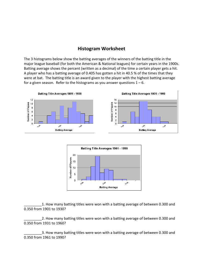
Histogram Worksheet The 3 histograms below show the batting averages of the winners of the batting title in the major league baseball (for both the American & National leagues) for certain years in the 1900s. Batting average shows the percent (written as a decimal) of the time a certain player gets a hit. A player who has a batting average of 0.405 has gotten a hit in 40.5 % of the times that they were at bat. The batting title is an award given to the player with the highest batting average for a given season. Refer to the histograms as you answer questions 1 – 6.

_________1. How many batting titles were won with a batting average of between 0.300 and 0.350 from 1901 to 1930? _________2. How many batting titles were won with a batting average of between 0.300 and 0.350 from 1931 to 1960? _________3. How many batting titles were won with a batting average of between 0.300 and 0.350 from 1961 to 1990?

4. If you were to find the mean of each of the winning batting averages for each time period, which time period do you think would have the highest mean? Explain. ____________________________________________________________________________________________________________________________________________________________________ 5. As the century progressed, what in general happened to the batting averages of the batting title winners? Explain. ____________________________________________________________________________________________________________________________________________________________________ ____________________________________________________________________________________________________________________________________________________________________ For questions 6 – 10, refer to the following 2 histograms. These histograms were made in an attempt to determine if William Shakespeare was really just a pen name for Sir Francis Bacon. (A pen name is a fake name used by another person when writing). A few scholars have had this idea and in order to determine if this was true, a researcher had to count the letters in every word of Shakespeare’s plays & Bacon’s writing (and you thought you had a lot of homework). Their results are recorded in the histograms below.

_________6. What percent of all Shakespeare’s words are 4 letters long? _________7. What percent of all Bacon’s words are 4 letters long? _________8. What percent of all Shakespeare’s words are more than 5 letters long? _________9. What percent of all Bacon’s words are more than 5 letters long? 10. Based on these histograms, do you think that William Shakespeare was really just a pen name for Sir Francis Bacon? Explain. _____________________________________________________________________________________________________________________________________________________________________________________________________________________

Suppose that the two histograms above show the sleeping habits of the teens at two different high schools. Wheatland High School is a small rural school consisting of 100 students while Urbandale High School is located in a large city and has 3,500 students. _________11. About what percent of the students at Wheatland get at least 8 hours of sleep

per night? _________12. About what percent of the students at Urbandale get at least 8 hours of sleep per night? _________13. Which high school has more actual students that sleep between 9 – 10 hours per night? _________14. Which high school has a higher median sleep time? 15. Wheatland’s percent of students who sleep between 8-9 hours a night is ________ % more than Urbandale’s percent of students who sleep between 8-9 hours per night. 16. Consider the type of data in the last two sets of problems (letters per word & sleep times).

_________a) Are letters per word qualitative or quantitative? _________b) Are sleep times qualitative or quantitative? _________c) Which data set is continuous? _________d) Which data set is discrete

17. The charts below shows the age of the actress & actor who won the Oscar for best

actress or actor during the first 30 years of the Academy Awards. Use the charts to make two histograms (one for winning actresses ages & one for winning actors ages) displaying this information. Use bin widths of ten years (0-9; 10-19; 20-29 etc.)

Year Age of

Winning Actress

Age of Winning

Actor 1928 22 42 1929 36 40 1930 28 62 1931 62 53 1932 32 35 1933 24 34 1934 29 33 1935 27 52 1936 27 41 1937 28 37 1938 30 38 1939 26 34 1940 29 32 1941 24 40 1942 34 43 Year Age of

Winning Actress

Age of Winning

Actor 1943 24 49 1944 29 41 1945 37 40 1946 30 49 1947 34 56 1948 34 41 1949 33 38 1950 28 38 1951 38 52 1952 45 51 1953 24 35 1954 26 30 1955 47 38 1956 41 41 1957 27 43

18. Write a short paragraph discussing what your two histograms reveal. ______________________________________________________________________________________________________________________________________________________________________________________________________________________________________________________________________________________________________________________________________________________________________________________________________________________________________________________________________________________________________________________________________________________________________________________________

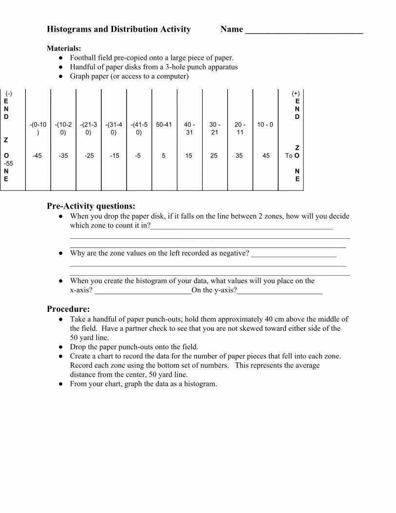
Histograms and Distribution Activity Name __________________________ Materials:

Football field pre­copied onto a large piece of paper. Handful of paper disks from a 3­hole punch apparatus Graph paper (or access to a computer)

(­) (+) E E N N D D ­(0­10

) ­(10­20)

­(21­30)

­(31­40)

­(41­50)

50­41 40 ­ 31

30 ­ 21

20 ­ 11

10 ­ 0

Z Z

O ­55

­45 ­35 ­25 ­15 ­5 5 15 25 35 45 To O

N N E E

Pre­Activity questions:

When you drop the paper disk, if it falls on the line between 2 zones, how will you decide which zone to count it in?_______________________________________________ _______________________________________________________________________________________________________________________________________________

Why are the zone values on the left recorded as negative? ______________________ _______________________________________________________________________ ________________________________________________________________________

When you create the histogram of your data, what values will you place on the x­axis? _________________________On the y­axis?______________________

Procedure: Take a handful of paper punch­outs; hold them approximately 40 cm above the middle of

the field. Have a partner check to see that you are not skewed toward either side of the 50 yard line.

Drop the paper punch­outs onto the field. Create a chart to record the data for the number of paper pieces that fell into each zone.

Record each zone using the bottom set of numbers. This represents the average distance from the center, 50 yard line.

From your chart, graph the data as a histogram.

Analysis questions 1. Draw the general shape of your histogram as a line graph:

Does the line graph have a characteristic shape? _________ If so, what is the general shape of this graph?________________________________ Explain why you think the graph is shaped this way: _____________________________

________________________________________________________________________ ________________________________________________________________________

2. Were there any ‘outlying’ values on your graph (beyond the general graph pattern or off the field)? _____________ If so, explain if these data points should be discarded: ________________________________________________________________________________________________________________________________________________

3. Brainstorm some ideas as to why some of the paper disks fell so much farther from the 50 yard line then others:

____________________________________________________________ ____________________________________________________________ ____________________________________________________________

4. How would the following scenarios affect the results of your histogram:

Height of the drop ­ ____________________________________________ _____________________________________________________________ _____________________________________________________________ Location of the drop in reference to the 50 yard line ­ __________________ _____________________________________________________________ _____________________________________________________________ Throwing the disks onto the field instead of dropping them ­ _____________ ______________________________________________________________ ______________________________________________________________

5. How can viewing a histogram be used to reconstruct the ‘history’ of the event that

occurred? ______________________________________________________________ ______________________________________________________________ ______________________________________________________________ ______________________________________________________________

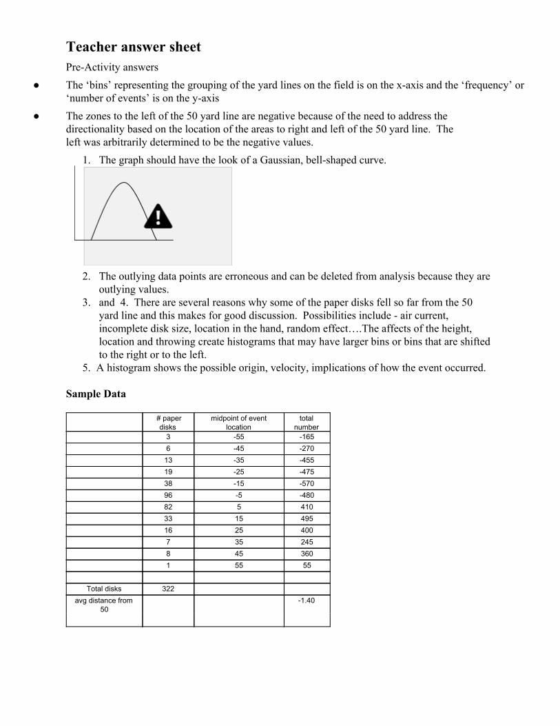
Teacher answer sheet Pre­Activity answers

The ‘bins’ representing the grouping of the yard lines on the field is on the x­axis and the ‘frequency’ or ‘number of events’ is on the y­axis

The zones to the left of the 50 yard line are negative because of the need to address the directionality based on the location of the areas to right and left of the 50 yard line. The left was arbitrarily determined to be the negative values.

1. The graph should have the look of a Gaussian, bell­shaped curve.

2. The outlying data points are erroneous and can be deleted from analysis because they are

outlying values. 3. and 4. There are several reasons why some of the paper disks fell so far from the 50

yard line and this makes for good discussion. Possibilities include ­ air current, incomplete disk size, location in the hand, random effect….The affects of the height, location and throwing create histograms that may have larger bins or bins that are shifted to the right or to the left.

5. A histogram shows the possible origin, velocity, implications of how the event occurred. Sample Data

# paper disks

midpoint of event location

total number

3 ­55 ­165 6 ­45 ­270 13 ­35 ­455 19 ­25 ­475 38 ­15 ­570 96 ­5 ­480 82 5 410 33 15 495 16 25 400 7 35 245 8 45 360 1 55 55

Total disks 322 avg distance from

50 ­1.40

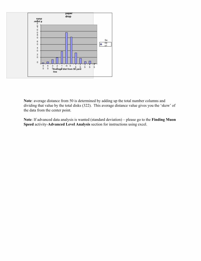
Note: average distance from 50 is determined by adding up the total number columns and dividing that value by the total disks (322). This average distance value gives you the ‘skew’ of the data from the center point. Note: If advanced data analysis is wanted (standard deviation) – please go to the Finding Muon Speed activity­Advanced Level Analysis section for instructions using excel.

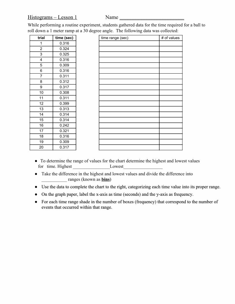
Histograms – Lesson 1 Name ________________________ While performing a routine experiment, students gathered data for the time required for a ball to roll down a 1 meter ramp at a 30 degree angle. The following data was collected:

trial time (sec) time range (sec) # of values 1 0.316 2 0.324 3 0.325 4 0.316 5 0.309 6 0.316 7 0.311 8 0.312 9 0.317 10 0.308 11 0.311 12 0.399 13 0.313 14 0.314 15 0.314 16 0.242 17 0.321 18 0.316 19 0.309 20 0.317

To determine the range of values for the chart determine the highest and lowest values for time. Highest ________________Lowest_________________

Take the difference in the highest and lowest values and divide the difference into ___________ ranges (known as bins)

Use the data to complete the chart to the right, categorizing each time value into its proper range. On the graph paper, label the x­axis as time (seconds) and the y­axis as frequency. For each time range shade in the number of boxes (frequency) that correspond to the number of

events that occurred within that range.

Analysis questions 1. What do you notice about the graphed results of the histogram?

2. Note the outlying data points. Are these valid points or should they be disregarded?

Why or why not?

3. What is binning?

4. What is on the y­axis of any histogram graph?

5. What is a histogram?

6. How is a histogram used to determine valid/invalid data?

7. Based on the histogram, what is the time for the ball to roll down the ramp?

8. Based on the histogram, what is the reasonable range of uncertainty in the time?

Teacher answer sheet ­ Histograms – Lesson 1

1. The data is grouped so that the most frequent values are a distinguishing peak on the graph. 2. The outlying data points are erroneous and can be deleted from the analysis of the the values. 3. Binning is a method of sorting data by clustering similar values and determining frequency. 4. The ‘frequency’ or ‘number of events’ is on the y­axis. 5. A histogram is a bar graph that shows how often events occurs within a bin/range. 6. A histogram is used to determine valid data by looking at the bulk of where the data falls and

identifying any outlying data that is can be removed. trial time

(sec) time range (sec) # of

values 1 0.316 0.240 ­ 0.248 1 2 0.324 0.249 ­ 0.257 3 0.325 0.258 ­ 0.266 4 0.316 0.267 ­ 0.275 5 0.309 0.276 ­ 0.284 6 0.316 0.285 ­ 0.293 7 0.311 0.294 ­ 0.302 8 0.312 0.303 ­ 0.311 5 9 0.317 0.312 ­ 0.320 10 10 0.308 0.321 ­ 0.329 3 11 0.311 0.330 ­ 0.328 12 0.399 0.339 ­ 0.347 13 0.313 0.348 ­ 0.356 14 0.314 0.357 ­ 0.365 15 0.314 0.366 ­ 0.374 16 0.242 0.375 ­ 0.383 17 0.321 0.384 ­ 0.392 18 0.316 0.393 ­ 0.401 1 19 0.309 20 0.317

Bin

Frequency

0.24 1 0.249 0 0.258 0 0.267 0 0.276 0 0.285 0 0.294 0 0.303 5 0.312 10 0.321 3 0.33 0 0.339 0 0.348 0 0.357 0 0.366 0 0.375 0 0.384 0 0.393 1 0.402 0

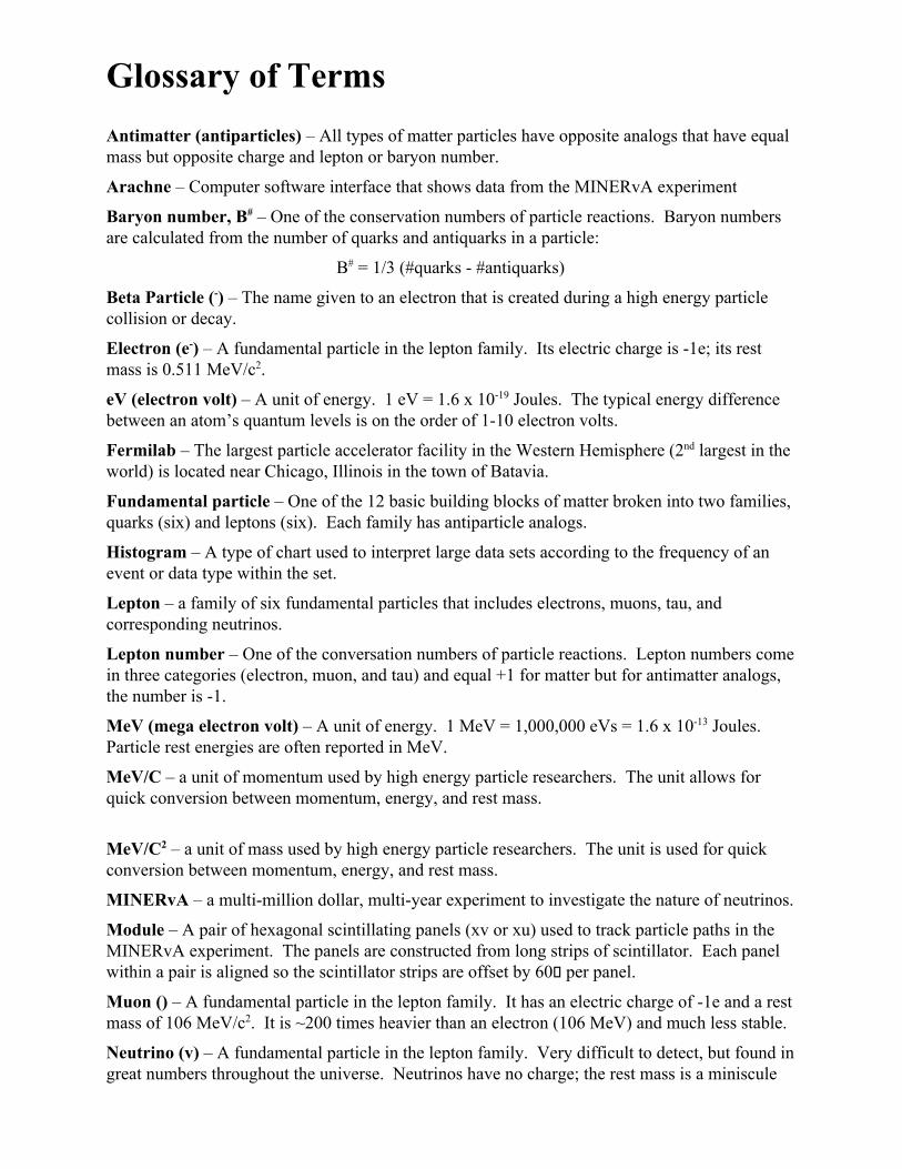
Glossary of Terms Antimatter (antiparticles) – All types of matter particles have opposite analogs that have equal mass but opposite charge and lepton or baryon number.

Arachne – Computer software interface that shows data from the MINERvA experiment

Baryon number, B# – One of the conservation numbers of particle reactions. Baryon numbers are calculated from the number of quarks and antiquarks in a particle:

B# = 1/3 (#quarks ­ #antiquarks)

Beta Particle (­) – The name given to an electron that is created during a high energy particle collision or decay.

Electron (e­) – A fundamental particle in the lepton family. Its electric charge is ­1e; its rest mass is 0.511 MeV/c2.

eV (electron volt) – A unit of energy. 1 eV = 1.6 x 10­19 Joules. The typical energy difference between an atom’s quantum levels is on the order of 1­10 electron volts.

Fermilab – The largest particle accelerator facility in the Western Hemisphere (2nd largest in the world) is located near Chicago, Illinois in the town of Batavia.

Fundamental particle – One of the 12 basic building blocks of matter broken into two families, quarks (six) and leptons (six). Each family has antiparticle analogs.

Histogram – A type of chart used to interpret large data sets according to the frequency of an event or data type within the set.

Lepton – a family of six fundamental particles that includes electrons, muons, tau, and corresponding neutrinos.

Lepton number – One of the conversation numbers of particle reactions. Lepton numbers come in three categories (electron, muon, and tau) and equal +1 for matter but for antimatter analogs, the number is ­1.

MeV (mega electron volt) – A unit of energy. 1 MeV = 1,000,000 eVs = 1.6 x 10­13 Joules. Particle rest energies are often reported in MeV.

MeV/C – a unit of momentum used by high energy particle researchers. The unit allows for quick conversion between momentum, energy, and rest mass.

MeV/C2 – a unit of mass used by high energy particle researchers. The unit is used for quick conversion between momentum, energy, and rest mass.

MINERvA – a multi­million dollar, multi­year experiment to investigate the nature of neutrinos.

Module – A pair of hexagonal scintillating panels (xv or xu) used to track particle paths in the MINERvA experiment. The panels are constructed from long strips of scintillator. Each panel within a pair is aligned so the scintillator strips are offset by 60 per panel.

Muon () – A fundamental particle in the lepton family. It has an electric charge of ­1e and a rest mass of 106 MeV/c2. It is ~200 times heavier than an electron (106 MeV) and much less stable.

Neutrino (v) – A fundamental particle in the lepton family. Very difficult to detect, but found in great numbers throughout the universe. Neutrinos have no charge; the rest mass is a miniscule

0.00005 MeV/c2.

Neutron (n0) – An electrically neutral subatomic particle commonly found in an atom’s nucleus. Made of 1 up quark and 2 down quarks (udd), it has a rest mass of 939 MeV.

NuMI Beam – a high energy neutrino beam in Fermilab that provides the stream of neutrino particles that initiate the reactions of interest in the MINERvA experiment.

Particle decay (beta, pion, muon, etc.) – The process mediated by the weak force that allows less stable particles to change identity to a more stable state.

Pion () – Any of several commonly produced particles in high energy reactions. Always composed of two quarks (up and/or down), a pion’s charge may be +1e, 0, or ­1e and its rest mass is approximately 140 MeV.

Quarks – A family of fundamental particles including the up, down, top, bottom, charm, and strange quark. These particles have charges of +2/3 e or ­1/3 e and have masses on the order of MeV’s.

Rest Mass – the minimum mass of a particle, describing the particle at rest. Every particle’s mass increases as it moves faster; this is in accordance with Einstein’s theory of relativity.

Scintillation – a process where a high energy particle dumps some of its energy as it passes through a special target. The chemicals in the special target convert some of the deposited energy into photon or light energy.

Standard Model – A broad physics theory that describes the existence of fundamental particles and forces in nature. This model describes and predicts the appearance of a whole “zoo” of exotic particles that have been observed in high energy particle accelerators.

Strong force – attractive force between quarks. It is the force responsible for holding all the positively charged protons together in the nucleus.

Weak force – an interaction between leptons or quarks that allows them to switch identities through very massive exchange particles called bosons. This force is responsible for nuclear fission or fusion reactions.

xu view – the information from a module a pair of panels in the MINERvA experiment oriented .

xv view ­ a pair of panels in the MINERvA experiment oriented to map a particles 3­D path through the target.

z­axis – the axis in space that runs straight through the MINERvA detector modules.