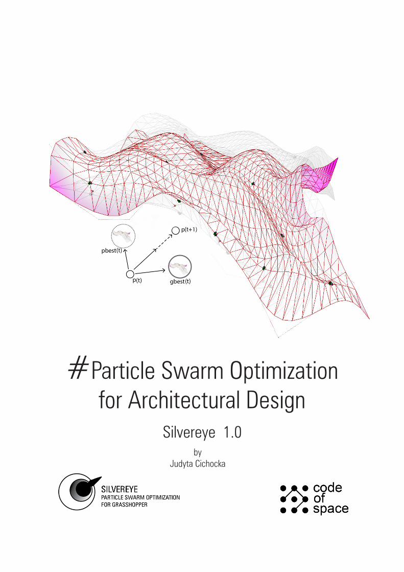
#Particle Swarm Optimization for Architectural Design

Silvereye 1.0by

Judyta Cichocka

This book produced and published digitally for public use. No part of this book may be reproduced in any manner whatsoever without permission from the author, except in the context of reviews.

© Code of Space. All rights reserved.

ISBN: 978-83-943176-1-4

1st edition, August 2016, Vienna

#Particle Swarm Optimization for Architectural Design

Silvereye 1.0

Judyta Cichocka

ISBN 978-83-943176-1-4

9 7 8 8 3 9 4 3 1 7 6 1 4

Content

1. Intoduction .....................................................................................................................3

1.1 Citing Silvereye.........................................................................................................4

1.2 Silvereye’s mission...................................................................................................4

2. Optimization of design problems ....................................................................................5

2.1 Background...............................................................................................................5

2.2 Method....................................................................................................................6

2.3 Visualization of the optimization process...................................................................7

3. Silvereye 1.0...................................................................................................................9

3.1 Installation..............................................................................................................9

3.2 Setting Up the Optimization process......................................................................10

3.3 Optimization process..............................................................................................14

3.4 Tuning Silvereye......................................................................................................17

4. Case Studies.................................................................................................................19

4.1 Travelling Salesman Problem (TSP).......................................................................19

4.2 Adjusting the roof geometry...................................................................................21

5. Acknowledgement........................................................................................................24

6. Bibliography...................................................................................................................25

#1 Introduction

Silvereye is an optimization solver, fully embedded in the parametric environment of Grasshop-

per which is a plug-in for the 3d modeling tool Rhinoceros. Silvereye is a result of a joint research be-

tween Wroclaw University of Technology (WRUT) and Victoria University of Wellington (VUW).

Silvereye 1.0 has been developed by:

Judyta Cichocka (WRUT, Faculty of Architecture, Department of History of Architecture, Arts and Technology),

Agata Migalska (WRUT, Faculty of Electronics),

Will Browne (VUW, School of Engineering and Computer Science)

Edgar Rodriguez (VUW, School of Architecture and Design).

Our team was the first to introduce an optimization solver based on Swarm Intelligence for architecture

and design (Cichocka et al. 2015).

We have developed, verified and tested the single objective optimization tool - Silvereye, which had its

beta release on 28.06.2016 and is now available to Grasshopper users for testing and feedback.

Silvereye is an optimization plug-in like Galapagos or Octopus. However, unlike these programs

that are based on Genetic Algotithms, Silvereye performs the optimization routine based the

Swarm Intelligence. It is dedicated for single-objective searches in solving real-world design pror-

blems. It is easy to use for non-experts, has been tailored to the needs of architects, design-

ers and engineers in the early design phase. Silvereye is a free version for non-commercial use only.

# 3

Figure 1. on the left: Silvereye bird – a native New Zealand specie. In late summer silvereyes gather into flocks and migrate to the north. source: australiangeographic.com.au on the right: Silvereye plug-in logotype.

# 4

Figure 2. Roof structure optimized with SIilvereye. The maximum nodal displacement for both initial and optimized design was calculated with FEM analysis under 1cm.

1.1. Citing Silvereye

In case you use Silvereye for your scientific work please cite the following papers:

Cichocka J.M., Migalska A., Browne W.N., Rodriguez E., 2016, “SILVEREYE- the implementation of Particle

Swarm Optimization (PSO) algorithm in a single objective optimization tool for Grasshopper” (n.p.)

Cichocka J., 2016, ‘Particle Swarm Optimization for Architectural Design – Silvereye 1.0’, Code of Space,

Vienna

1.2 Silvereye’s Mission

An optimization process is a great solution for designing energy efficient and sustainable architecture.

Building sustainable lives in harmony with the ecosystems and local resources requires a bottom-up ap-

proach. Environmental and economic challenges have multiple features that can be optimized. New opti-

mization tools can facilitate aiding and solving architectural design problems such as daylight availability,

material use and construction waste, logistical efficiency, fabrication rationalization, cost-effectiveness

and other design aspects. Robust optimization processes significantly reduce carbon-footprint, reduce the

material use and increase the energy-efficiency.

Goal of sustainable design is to eliminate negative environmental impact completely through skilful, sensi-

tive design. Silvereye is a measure to achieve this goal.

# 5

#2 Optimization of design problems

By difficult optimization problem we understand a problem which (Michalewicz & Fogel 2004):

- has such a high number of possibile solutions that cheking all of them would take ages

- cannot be simiplified, as simplification of the problem would lead to discovery of useless solutions

- might have several optimal solutions

- is contrainted and discovering even one feasible solution might be difficult

Real-world design optimization problems are usually too difficult for the analytical methods to solve in finite

time. When classic methods fail to find any exact solution, heuristics are employed - techniques that are

not guaranteed to find an optimal solution but are at least capable of finding approximate solutions.

2.1 Background

In 1960’s a heuristic that mimics the process of natural selection, Genetic Algorithm (GA), was developed

for solving diffucult, real-world problems. A population reproduces by means of gene crossings and muta-

tions in order to create better offspring and repeats that reproduction until termination criteria are met. In

1994 a concept of Swarm Intelligence (SI) emerged (Millonas 1994), inspired by the movement of organ-

isms in a bird flock or fish school. A swarm is formed of the particles, whose movement are influenced by

their own knowledge as well as by the knowledge of the whole swarm. It was soon discovered that Swarm

Intelligence approach can be used to efficiently solve optimization problems and so Particle Swarm Opti-

mization (PSO) algorithm for optimizing a single objective optimization problems was proposed (Kennedy

& Eberhart 1995). Through extensive research it has been shown that for many classes of problems PSO

converges to the optimal solution quicker than GA, i.e. PSO requires less iterations.

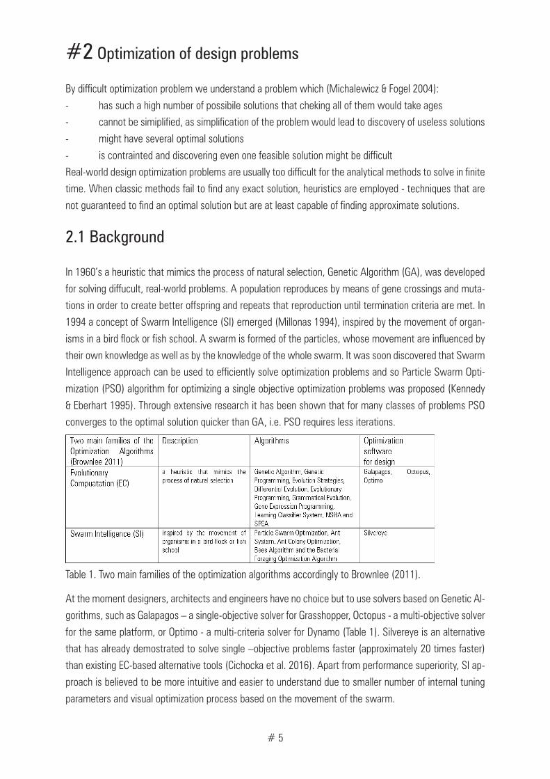
At the moment designers, architects and engineers have no choice but to use solvers based on Genetic Al-

gorithms, such as Galapagos – a single-objective solver for Grasshopper, Octopus - a multi-objective solver

for the same platform, or Optimo - a multi-criteria solver for Dynamo (Table 1). Silvereye is an alternative

that has already demostrated to solve single –objective problems faster (approximately 20 times faster)

than existing EC-based alternative tools (Cichocka et al. 2016). Apart from performance superiority, SI ap-

proach is believed to be more intuitive and easier to understand due to smaller number of internal tuning

parameters and visual optimization process based on the movement of the swarm.

Table 1. Two main families of the optimization algorithms accordingly to Brownlee (2011).

# 6

2.2 Method

Swarm Intelligence implementation.

Swarm Optimization technique was selected for implementation as it “seeks to make things simpler rather

than more complex” (Kennedy & Eberhart 1995). The algorithm implemented in the Silvereye meets all five

basic principles of Swarm Intelligence described by Millonas (Millonas 1994). The PSO algorithm is imple-

mented in its native form with added internal weight factors, which were introduced to prevent velocities

becoming too large (Shi & Eberhart 1998) and has following pseudo code:

For each particle Initialize particle

END

Do For each particle Calculate fitness value If the fitness value is better than the best fitness value (pBest) in history set current value as the new pBest End Choose the particle with the best fitness value of all the particles as the gBest

For each particle Calculate particle velocity according equation(a) Update particle position according equation(b) End

Where:

v[ ] = v[ ] + w*c1 * rand( ) * (pbest[ ] - present[ ]) + w * c2 * rand( ) * (gbest[ ] - present[ ] ) (a)

present[ ] = persent[ ] + v[ ] (b)

The above pseudo code was adopted from: http://www.swarmintelligence.org/, where pbest –the best

solution that has been achieved by the particle so far and gbest - the best value obtained so far by any

particle in the population. It adopts the following internal parameters:

w – an interia coefficient (w= 0.3)

c1, c2 – learning factors (c1 and c2 = 2)

rand( ) - uniformly distributed random variables within range [0, 1]

(Shi & Eberhart, 1998)

# 7

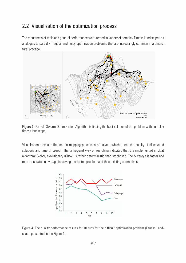
2.2 Visualization of the optimization process

The robustness of tools and general performance were tested in variety of complex Fitness Landscapes as

analogies to partially irregular and noisy optimization problems, that are increasingly common in architec-

tural practice.

Visualizations reveal difference in mapping processes of solvers which affect the quality of discovered

solutions and time of search. The orthogonal way of searching indicates that the implemented in Goat

algorithm: Global, evolutionary (CRS2) is rather deterministic than stochastic. The Silvereye is faster and

more accurate on average in solving the tested problem and then existing alternatives.

Figure 4. The quality performance results for 10 runs for the difficult optimization problem (Fitness Land-

scape presented in the Figure 1).

Figure 3. Particle Swarm Optimizartion Algorithm is finding the best solution of the problem with complex fitness landscape.

# 8

Figure 5. Visualization of mapping processes in single objective optimization. Source:(Cichocka et al. 2015)

#9

#3 Silvereye 1.0

3.1 Installation

You can download Silvereye from: http://www.food4rhino.com/project/silvereye?etx

Follow the instructions to install Silvereye plug-in:

1. Open Rhino and Grasshopper

2. To install Silvereye go to Components Folder (directly from Grasshopper => File/Special Folders/

Components Folder or you can find it following the path: C:\Users\*\AppData\Roaming\Grasshopper\Librar-

ies

3. Copy and paste (drag and drop) Silverye.gha and SwarmOptimization.dll to the Components Folder

4. Right click on the both files and choose “Unblock”

5. Restart Rhino and Grasshopper

6. Silvereye component can be found in the Params / Utils category.

7. Place the Silvereye on the canvas and enjoy! Optimize everyday!

8. Please find a few optimization exercises attached in the folder “exercises”.

9. User documentation can be found in the docs folder.

# 10

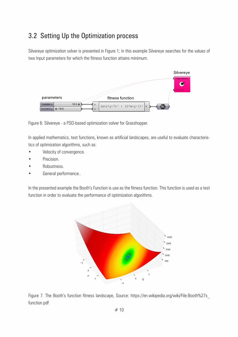
3.2 Setting Up the Optimization process

Silvereye optimization solver is presented in Figure 1; in this example Silvereye searches for the values of

two Input parameters for which the fitness function attains minimum.

Figure 6: Silvereye - a PSO-based optimization solver for Grasshopper.

In applied mathematics, test functions, known as artificial landscapes, are useful to evaluate characteris-

tics of optimization algorithms, such as:

• Velocity of convergence.

• Precision.

• Robustness.

• General performance..

In the presented example the Booth’s Function is use as the fitness function. This function is used as a test

function in order to evaluate the performance of optimization algorithms.

Figure 7. The Booth’s function fitness landscape, Source: https://en.wikipedia.org/wiki/File:Booth%27s_

function.pdf

# 11

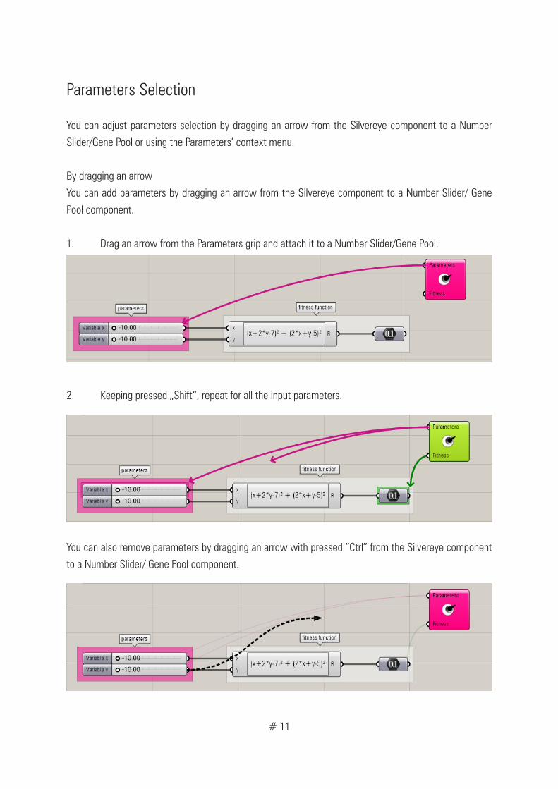
Parameters Selection

You can adjust parameters selection by dragging an arrow from the Silvereye component to a Number

Slider/Gene Pool or using the Parameters’ context menu.

By dragging an arrow

You can add parameters by dragging an arrow from the Silvereye component to a Number Slider/ Gene

Pool component.

1. Drag an arrow from the Parameters grip and attach it to a Number Slider/Gene Pool.

2. Keeping pressed „Shift“, repeat for all the input parameters.

You can also remove parameters by dragging an arrow with pressed “Ctrl” from the Silvereye component

to a Number Slider/ Gene Pool component.

#12

By context menu actions

To open a context menu, right click on the Parameters label on the Silvereye component.

1. You can add all the Number Sliders/Gene Pools in the GH document to the Silvereye’s Parameters. You

can also remove all the sliders from the Parameters.

2. You can select several Number Sliders/ Gene Pools and add this selection to Silvereye’s Parameters.

3. In a similar manner you can remove selected Number Sliders/Gene Pools from Silvereye’s Parameters.

4. Individual Number Sliders/Gene Pools can be removed from the Silvereye’s parameters. Mouse over on the input’s name to highlight it.

# 13

Fitness Value Selection

Once you connected the parameters to the Silvereye component, you have to plug-in the fitness function

that evaluates every discovered by the algorithm solution during optimization process. Connecting the firm-

ness value is simple and similar to connecting the design parameters, just follow the below instructions.

1. Fitness function value has to be stored in the Number component (Params/Primitive/Number)

2. Connect the fitness value by dragging an arrow from the Fitness grip to your Number component.

The green arrow should indicate the right connection. Now the values of the firmness function is read by

Silvereye directly from the Number component.

#14

3.3 Optimization process

Once you connected the Parameters and Fitness, you can start optimization process. Double click on the

Silvereye component to open the Silvereye Editor. You could adjust the Settings or leave them default and

go straight to the Optimization tab.

Objective - is the fitness goal. You can maximize or minimize your fitness function. As default Silvereye searches for the global minimum value of the plugged fitness function.

Iterations – set a number of iteration that solver should go through.

Max Velocity - is a “maximum jump” allowed between val-ues on the Number Sliders and the Gene Pools selected for the optimization process in every iteration (for example, if Number Slider has domain <-10.00,10.00>, the Max Veloc-ity 4 means that from the value 0.00 in the current iteration, Silvereye can explore values in the domain <-4.00,4.00> in the next iteration, as particle can maximally move 4 units in any direction). This rule applies to all connected Number Sliders and Gene Pools.

Runtime Limit – optimization process can be limited in time, check Runtime Limit checkbox and set the time. Leaving zero means no time limit.

Swarm Size – number of particles in the swarm (it is a num-ber of calculated solutions per iteration)Use Initial Position – Silvereye will start the optimization procedure from the values on the Number Sliders/Gene Pools, it means that current solution will be included in the first iteration

To save your setting for the next optimization run, click Save and Close.More about tuning Silvereye can be found in the paragraph 3.4 Tuning Silvereye.

To save your setting for the next optimization run, click Save and Close. More about tuning Silvereye can

be found in the paragraph 3.4 Tuning Silvereye.

#15

Silvereye Editor - Optimization

The PSO-based is a heuristic process, therefore try to run optimization several times to obtain different

result.

Once all the settings are adjusted, you can start the Optimization process. Go to Optimization tab in the

Silvereye Editor and press Start button.

If Parameters or Fitness is not connected to Silvereye component, you will get below alert after pressing

Start button. Otherwise the optimization run starts.

Press Start button in the Optimization tab in order to start optimization process. The Editor will be blocked

until the optimization process is finished.

#16

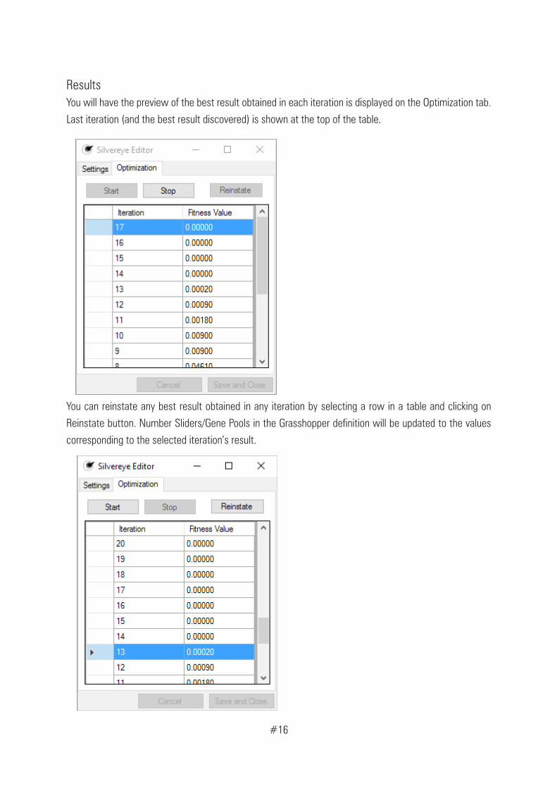
ResultsYou will have the preview of the best result obtained in each iteration is displayed on the Optimization tab.

Last iteration (and the best result discovered) is shown at the top of the table.

You can reinstate any best result obtained in any iteration by selecting a row in a table and clicking on

Reinstate button. Number Sliders/Gene Pools in the Grasshopper definition will be updated to the values

corresponding to the selected iteration’s result.

# 17

3.4 Tuning Silvereye

Numerous studies exist on the adjusting internal tuning parameters. A comprehensive survey of such stud-

ies was done by Carlisle and Dozier (2001). The first version of Silvereye adopts the standard set of set-

tings and the internal tuning parameters. The momentum coefficient for the whole swarm (w) and learning

factors (c1,c2) are constant in the algorithm and not adjustable for the user. For the implemented values in

the Silvereye setup check the paragraph: 2.2 Method. The Maximum velocity (Vmax) parameter and the

Swarm Size are fully adjustable by user in the Grasshopper interface..

Maximum Velocity

Maximum Velocity (Vmax) sets an upper bound for the velocity component. The maximum velocity might

be understood as the “maximum jump” allowed between values on the number sliders and the gene pools

selected for the optimization process in every iteration. Therefore, the maximum value of the velocity

(Vmax) is individual to each design problem, depending on the range of selected sliders/gene pools. It was

observed that the most efficient maximum velocities should be between 5% and 50% of the range of the

design parameters selected for the optimization (Cichocka et al. 2016).

Number of particles

The default swarm size is set to 20 particles. The recommended by Browlee (2011) swarm size is between

20 and 40 particles. The higher number of particles means denser sampling of the fitness landscape,

therefore decrease the chances to miss good solutions or get stuck in the local optima. If discovering

the closest result to the global optima (or global optima itself) is our priority, increasing the swarm size is

recommended. However, it has to be mentioned that computational expensiveness depends on the size of

the population. The larger the swarm, the longer the calculation per iteration.

Runtime Limit

The research on the Meiso no Mori Crematorium roof shape optimization(Cichocka et al. 2016) suggests

that first 15 minutes is crucial in the longer optimization runs. This fact is correct both for Silvereye and

tested alternatives: Octopus and Galapagos. This time may vary from problem to problem and depends on

the singular calculation time for one solution.

For example, if calculation of the solution is time-consuming like 1 minute per single solution. In the first

iteration 20 particles calculate their fitness values for their current parameters set-up. To go through 5

iterations to get some optimized result, 100 solutions have to be calculated. It means that for somehow

reasonable result we should wait about 100 minutes.

# 18

Figure 8. Graph of the structural performance improvement in time during 8-hour tests. (Cichocka et al.

2016)

Including your solution into optimization

In the Silvereye Editor you can check “Use Initial Positions”. Silvereye will start the search from the current

values on the Number Sliders/Gene Pools. It does not mean that it will search just locally. It means that our

solution will be included in the first iteration, and if Silvereye does not discover other better solution, it will

tend to find one close to one suggested by the user.

Local Search

If would like to proceed with more local search (we found manually a shape/geometry/architectural solu-

tion that we like, however maybe it can be improved just slightly), we can follow the below procedure.

1. narrow down the Number Sliders/Gene Pools domains (Right click on the Number Slider/Edit and

adjust the Min and Max values in the Numeric domain).

2. After that check ‘Use initial positions’ checkbox

3. Change the Max Velocity to a very small number.

# 19

#4 Case Studies

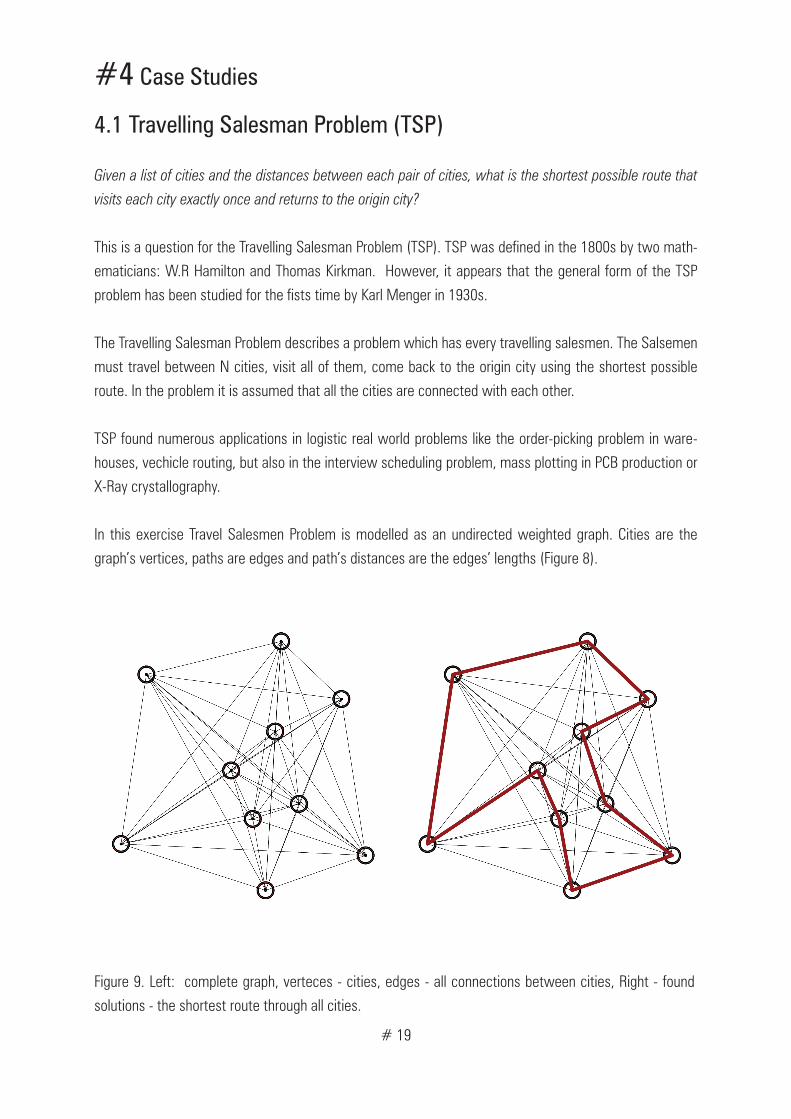
4.1 Travelling Salesman Problem (TSP)

Given a list of cities and the distances between each pair of cities, what is the shortest possible route that

visits each city exactly once and returns to the origin city?

This is a question for the Travelling Salesman Problem (TSP). TSP was defined in the 1800s by two math-

ematicians: W.R Hamilton and Thomas Kirkman. However, it appears that the general form of the TSP

problem has been studied for the fists time by Karl Menger in 1930s.

The Travelling Salesman Problem describes a problem which has every travelling salesmen. The Salsemen

must travel between N cities, visit all of them, come back to the origin city using the shortest possible

route. In the problem it is assumed that all the cities are connected with each other.

TSP found numerous applications in logistic real world problems like the order-picking problem in ware-

houses, vechicle routing, but also in the interview scheduling problem, mass plotting in PCB production or

X-Ray crystallography.

In this exercise Travel Salesmen Problem is modelled as an undirected weighted graph. Cities are the

graph’s vertices, paths are edges and path’s distances are the edges’ lengths (Figure 8).

Figure 9. Left: complete graph, verteces - cities, edges - all connections between cities, Right - found

solutions - the shortest route through all cities.

# 20

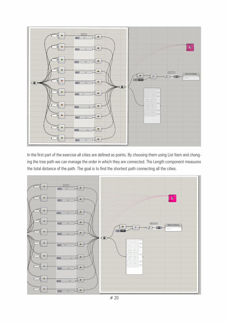
In the first part of the exercise all cities are defined as points. By choosing them using List Item and chang-

ing the tree path we can manage the order in which they are connected. The Length component measures

the total distance of the path. The goal is to find the shortest path connecting all the cities.

# 21

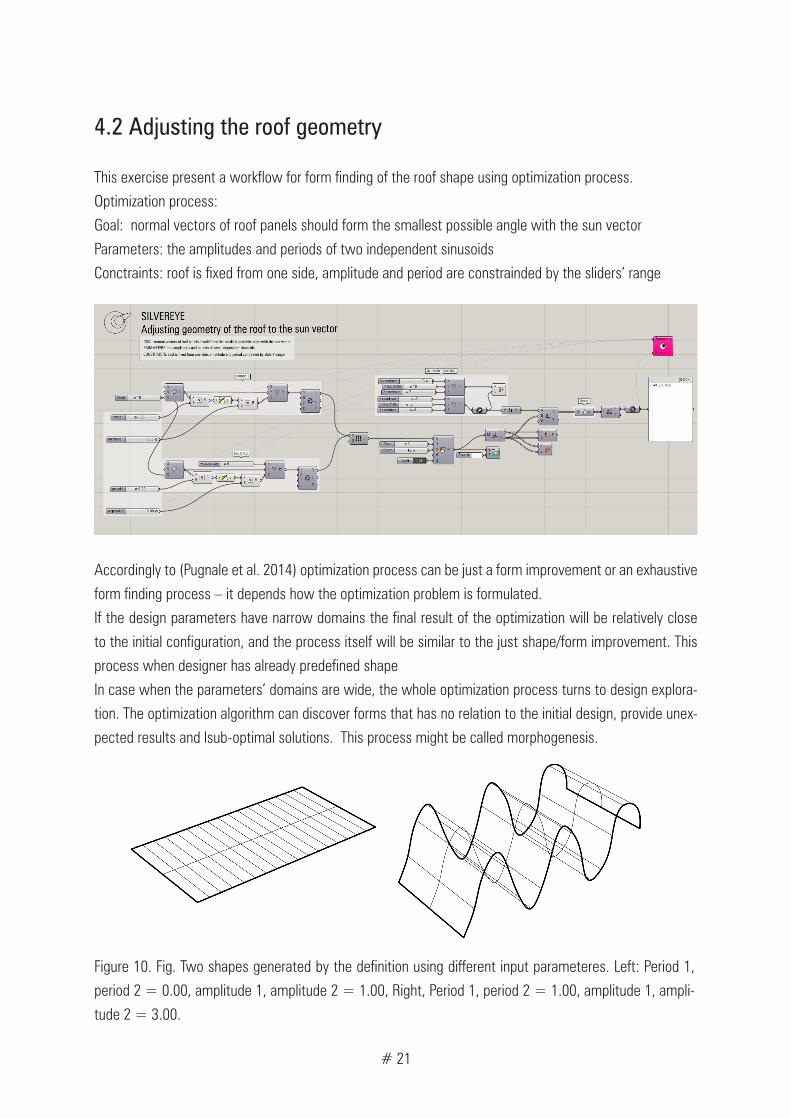
4.2 Adjusting the roof geometry

This exercise present a workflow for form finding of the roof shape using optimization process.

Optimization process:

Goal: normal vectors of roof panels should form the smallest possible angle with the sun vector

Parameters: the amplitudes and periods of two independent sinusoids

Conctraints: roof is fixed from one side, amplitude and period are constrainded by the sliders’ range

Accordingly to (Pugnale et al. 2014) optimization process can be just a form improvement or an exhaustive

form finding process – it depends how the optimization problem is formulated.

If the design parameters have narrow domains the final result of the optimization will be relatively close

to the initial configuration, and the process itself will be similar to the just shape/form improvement. This

process when designer has already predefined shape

In case when the parameters’ domains are wide, the whole optimization process turns to design explora-

tion. The optimization algorithm can discover forms that has no relation to the initial design, provide unex-

pected results and lsub-optimal solutions. This process might be called morphogenesis.

Figure 10. Fig. Two shapes generated by the definition using different input parameteres. Left: Period 1,

period 2 = 0.00, amplitude 1, amplitude 2 = 1.00, Right, Period 1, period 2 = 1.00, amplitude 1, ampli-

tude 2 = 3.00.

# 22

1. Definition of two independant sinusoids

2. Creation of the NURBS surface.

3. NURBS to MESH geometry with Mesh Sur-face Component.

4. Normal vectors with Face Normals Comonent.

OPTIMIZATION

5. The discovered solution.

# 23

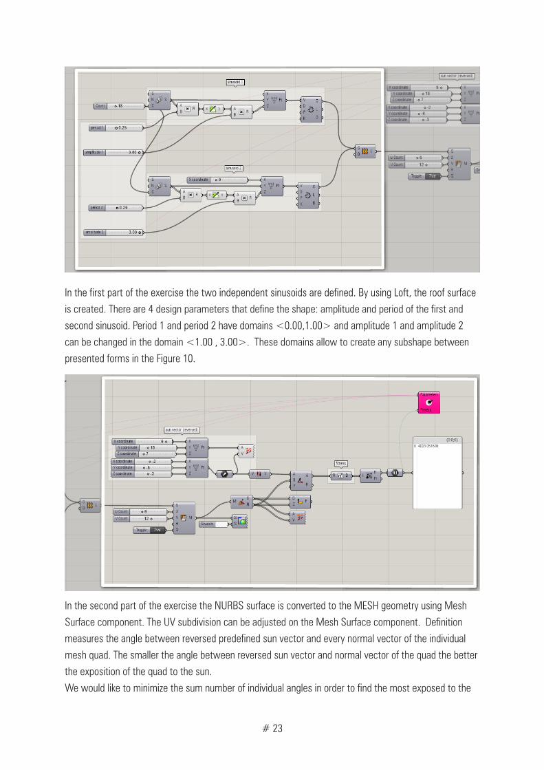
In the first part of the exercise the two independent sinusoids are defined. By using Loft, the roof surface

is created. There are 4 design parameters that define the shape: amplitude and period of the first and

second sinusoid. Period 1 and period 2 have domains <0.00,1.00> and amplitude 1 and amplitude 2

can be changed in the domain <1.00 , 3.00>. These domains allow to create any subshape between

presented forms in the Figure 10.

In the second part of the exercise the NURBS surface is converted to the MESH geometry using Mesh

Surface component. The UV subdivision can be adjusted on the Mesh Surface component. Definition

measures the angle between reversed predefined sun vector and every normal vector of the individual

mesh quad. The smaller the angle between reversed sun vector and normal vector of the quad the better

the exposition of the quad to the sun.

We would like to minimize the sum number of individual angles in order to find the most exposed to the

# 24

#5 Acknowledgement

This work would not have been possible without Agata Migalska, who properly implemented the Particle

Swarm Optimization Algorithm in the Grasshopper3d framework using C# language for custom compo-

nent scripting. Agata has also proposed the Travelling Salseman Problem as an exercise for this booklet

and assisted in the editing and proofreading in some parts of the book.

I am especially indebted to Dr. Will Browne, who has encouraged us to implement Particle Swarm Opti-

mization in particular and who worked actively to provide us with the protected academic time to pursue

Silvereye release.

I would like to express my gratitude to the people who saw me through this book; to all those who pro-

vided support, talked things over, read, wrote, offered comments, allowed me to quote their remarks and

assisted in the editing and proofreading.

The presented in the book research was financially supported by European Union within the “THELXINOE:

Erasmus Euro-Oceanian Smart City Network” grant.

# 25

#6 Bibliography

Brownlee, J., 2011. Clever Algorithms. Nature-Inspired Programming Recipes,

Cichocka J.M., Migalska A., Browne W.N., Rodriguez E., 2016, “SILVEREYE- the implementation of Particle

Swarm Optimization (PSO) algorithm in a single objective optimization tool for Grasshopper” (n.p.)

Cichocka, J.M., Browne, W.N. & Rodriguez, E., 2015. Evolutionary Optimization Processes As Design Tools : In Proceedings of 31th International PLEA Conference ARCHITECTURE IN (R)EVOLUTION, Bologna 9-11 September 2015.

Kennedy, J. & Eberhart, R., 1995. Particle swarm optimization. Neural Networks, 1995. Proceedings., IEEE International Conference on, 4, pp.1942–1948 vol.4.

Michalewicz, Z. & Fogel, B.D., 2004. How to Solve It: Modern Heuristics Second, Re., Springer.

Millonas, M.M., 1994. Swarms, Phase Transitions, and Collective Intelligence. Santa Fe Institute Stud-ies in the Sciences of Complexity-Proceedings Volume-, p.30. Available at: http://arxiv.org/abs/adap-org/9306002.

Pugnale, A., Echengucia, T. & Sassone, M., 2014. Computational morphogenesis. Design of freeform sur-faces. In S. Adriaenssens et al., eds. Shell Structures for Architecture. Form-finding and Optimization. Routledge.

Shi, Y. & Eberhart, R.C., 1998. A modified particle swarm optimizer. In Congress on Evolutionary Computa-tion. pp. 69–73.

ISBN 978-83-943176-1-4

9 7 8 8 3 9 4 3 1 7 6 1 4