Particle Swarm Optimization - Georgia Southern … · Particle Swarm Optimization Applications in Parameterization of Classiﬁers James Blondin [email protected] Armstrong Atlantic

Particle Swarm OptimizationApplications in Parameterization of Classifiers

James Blondin

[email protected]

Armstrong Atlantic State University

Particle Swarm Optimization – p. 1

Outline

• Introduction• Canonical PSO Algorithm• PSO Algorithm Example• Classifier Optimization• Conclusion


Particle Swarm Optimization

Particle Swarm Optimization (PSO) is a

• swarm-intelligence-based• approximate• nondeterministic

optimization technique.


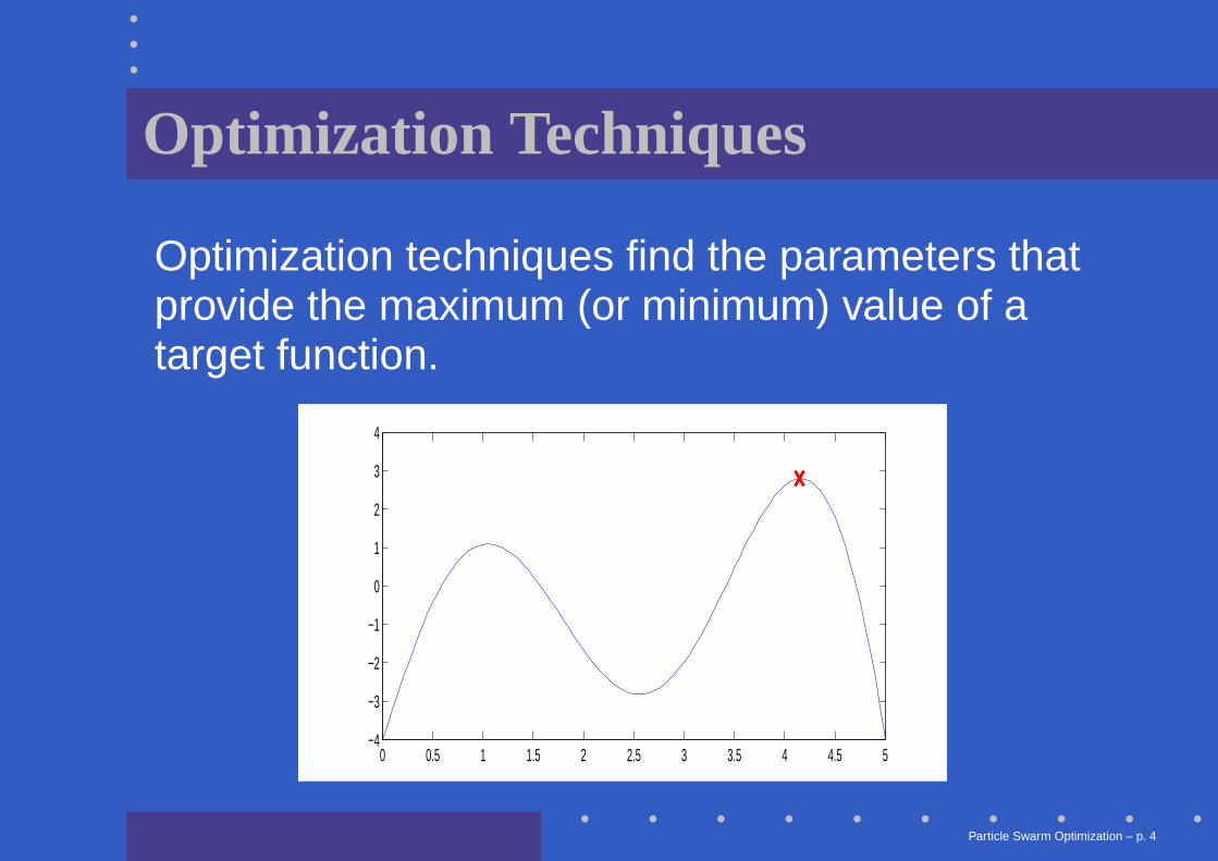
Optimization Techniques

Optimization techniques find the parameters thatprovide the maximum (or minimum) value of atarget function.

0 0.5 1 1.5 2 2.5 3 3.5 4 4.5 5−4

−3

−2

−1

0

1

2

3

4


Uses of Optimization

In the field of machine learning, optimizationtechniques can be used to find the parametersfor classification algorithms such as:

• Artificial Neural Networks• Support Vector Machines

These classification algorithms often require theuser to supply certain coefficients, which oftenhave to be found by trial and error or exhaustivesearch.


Canonical PSO Algorithm



Origins of PSO

PSO was first described by James Kennedy andRussell Eberhart in 1995.

Derived from two concepts:

• The observation of swarming habits ofanimals such as birds or fish

• The field of evolutionary computation (suchas genetic algorithms)


PSO Concepts

• The PSO algorithm maintains multiplepotential solutions at one time

• During each iteration of the algorithm, eachsolution is evaluated by an objective functionto determine its fitness

• Each solution is represented by a particle inthe fitness landscape (search space)

• The particles “fly” or “swarm” through thesearch space to find the maximum valuereturned by the objective function


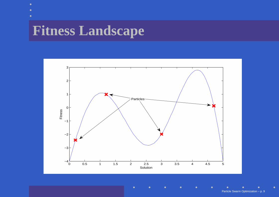
Fitness Landscape

0 0.5 1 1.5 2 2.5 3 3.5 4 4.5 5−4

−3

−2

−1

0

1

2

3

Solution

Fitn

ess

Particles


Maintained Information

Each particle maintains:

• Position in the search space (solution andfitness)

• Velocity• Individual best position

In addition, the swarm maintains its global bestposition.


Canonical PSO Algorithm

The PSO algorithm consists of just three steps:

1. Evaluate fitness of each particle

2. Update individual and global bests

3. Update velocity and position of each particle

These steps are repeated until some stoppingcondition is met.


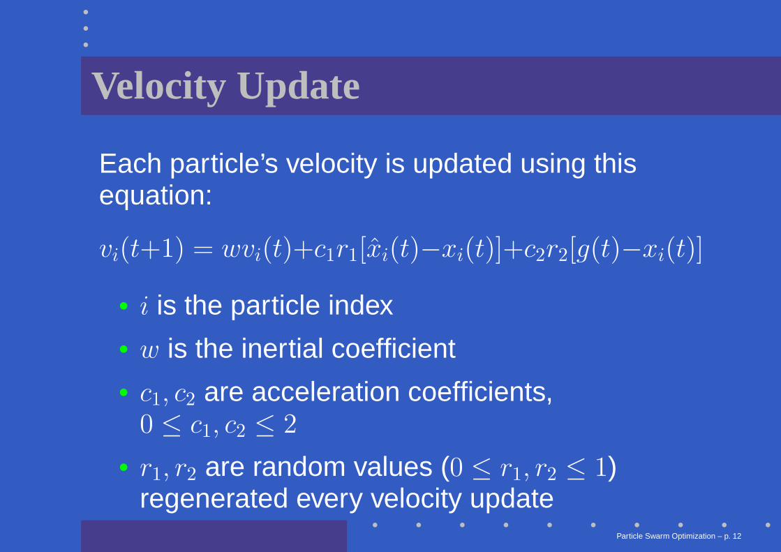
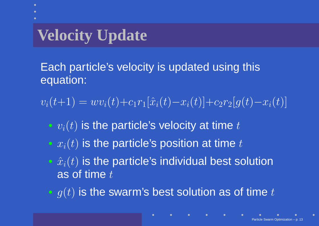
Velocity Update

Each particle’s velocity is updated using thisequation:

vi(t+1) = wvi(t)+c1r1[x̂i(t)−xi(t)]+c2r2[g(t)−xi(t)]

• i is the particle index• w is the inertial coefficient• c1, c2 are acceleration coefficients,

0 ≤ c1, c2 ≤ 2

• r1, r2 are random values (0 ≤ r1, r2 ≤ 1)regenerated every velocity update


Velocity Update

Each particle’s velocity is updated using thisequation:


• vi(t) is the particle’s velocity at time t

• xi(t) is the particle’s position at time t

• x̂i(t) is the particle’s individual best solutionas of time t

• g(t) is the swarm’s best solution as of time t


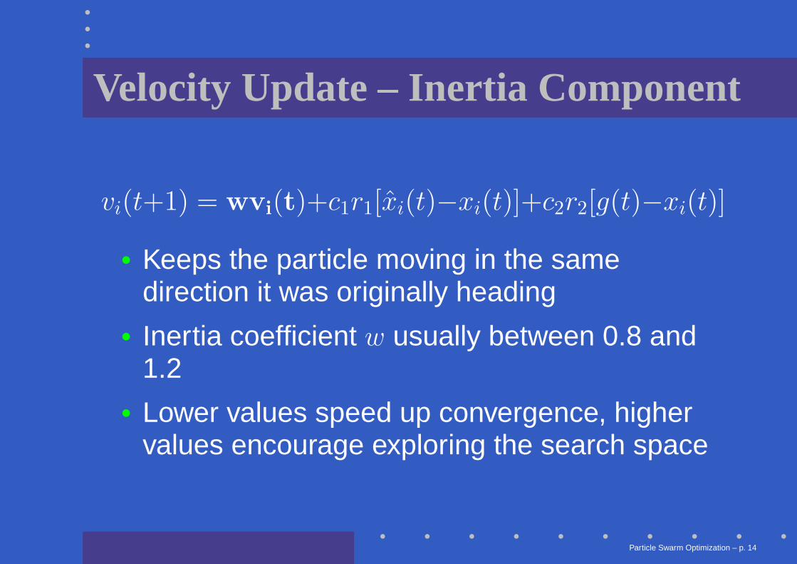
Velocity Update – Inertia Component


• Keeps the particle moving in the samedirection it was originally heading

• Inertia coefficient w usually between 0.8 and1.2

• Lower values speed up convergence, highervalues encourage exploring the search space


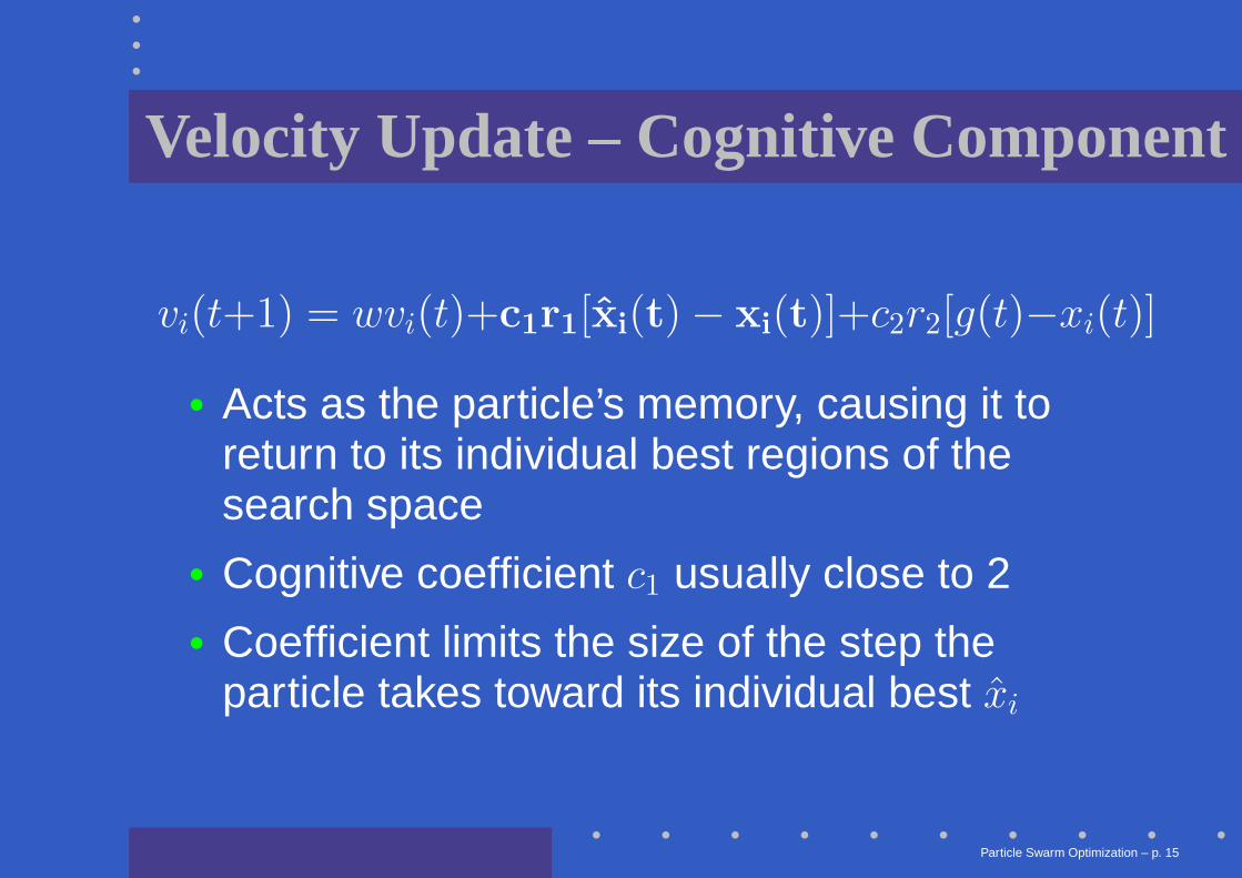
Velocity Update – Cognitive Component

vi(t+1) = wvi(t)+c1r1[x̂i(t) − xi(t)]+c2r2[g(t)−xi(t)]

• Acts as the particle’s memory, causing it toreturn to its individual best regions of thesearch space

• Cognitive coefficient c1 usually close to 2• Coefficient limits the size of the step the

particle takes toward its individual best x̂i


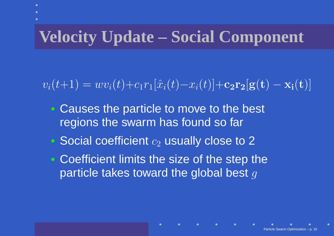
Velocity Update – Social Component

vi(t+1) = wvi(t)+c1r1[x̂i(t)−xi(t)]+c2r2[g(t) − xi(t)]

• Causes the particle to move to the bestregions the swarm has found so far

• Social coefficient c2 usually close to 2• Coefficient limits the size of the step the

particle takes toward the global best g


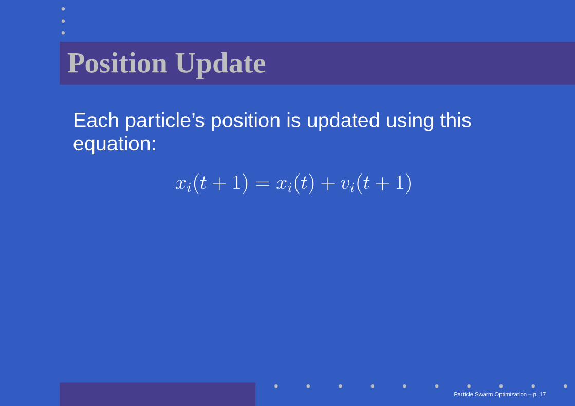
Position Update

Each particle’s position is updated using thisequation:

xi(t + 1) = xi(t) + vi(t + 1)


PSO Algorithm Example



PSO Algorithm Redux

Repeat until stopping condition is met:

1. Evaluate fitness of each particle

2. Update individual and global bests

3. Update velocity and position of each particle


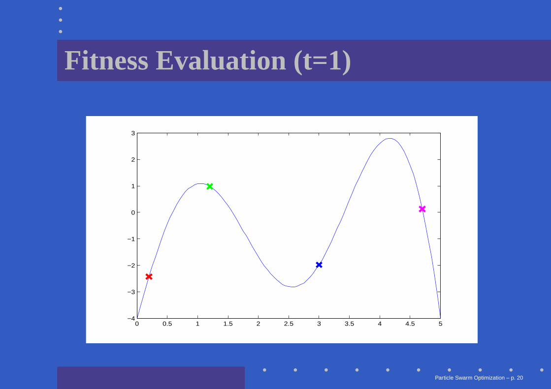
Fitness Evaluation (t=1)

0 0.5 1 1.5 2 2.5 3 3.5 4 4.5 5−4

−3

−2

−1

0

1

2

3


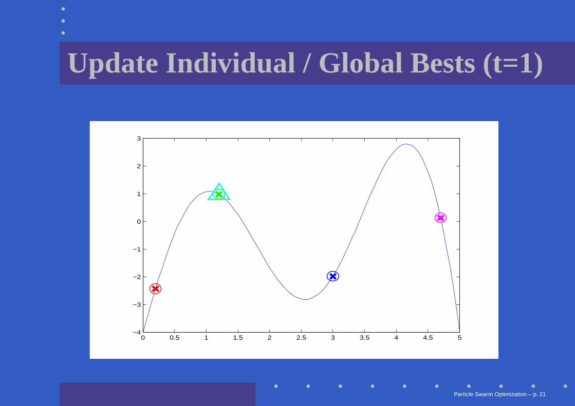
Update Individual / Global Bests (t=1)

0 0.5 1 1.5 2 2.5 3 3.5 4 4.5 5−4

−3

−2

−1

0

1

2

3


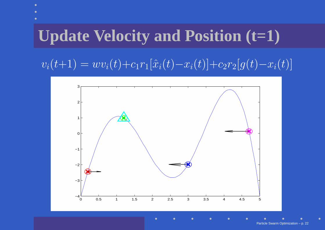
Update Velocity and Position (t=1)


0 0.5 1 1.5 2 2.5 3 3.5 4 4.5 5−4

−3

−2

−1

0

1

2

3


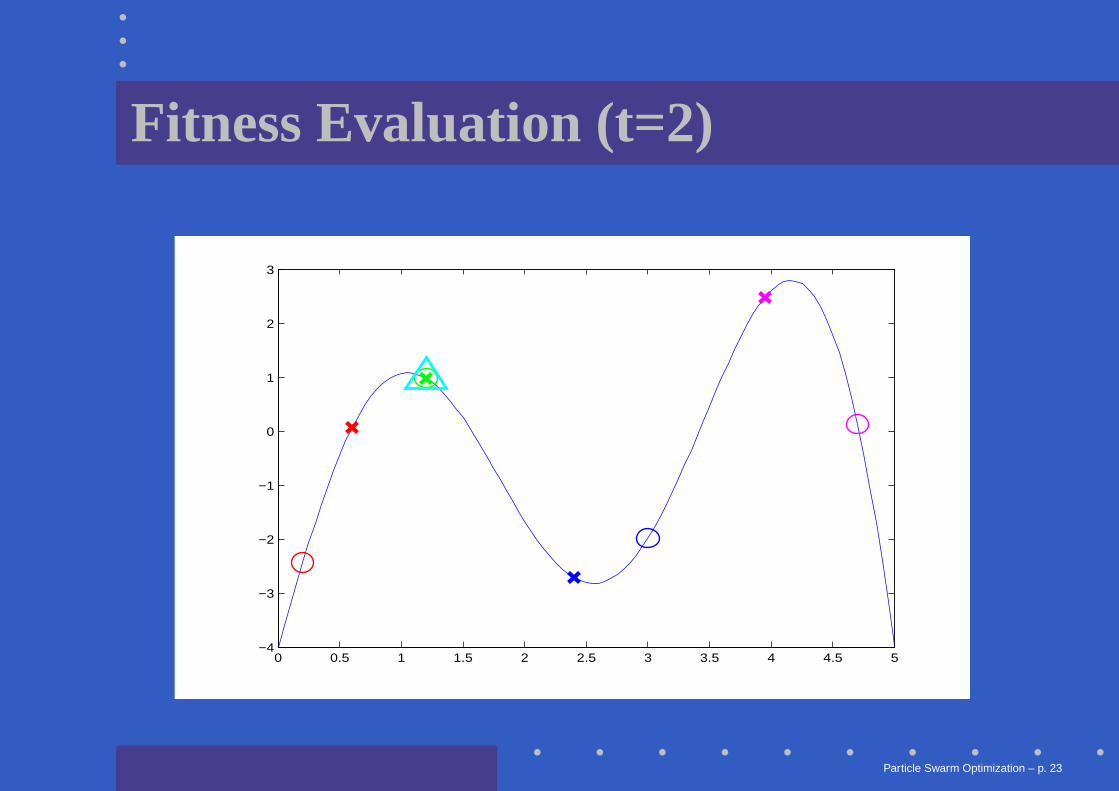
Fitness Evaluation (t=2)

0 0.5 1 1.5 2 2.5 3 3.5 4 4.5 5−4

−3

−2

−1

0

1

2

3


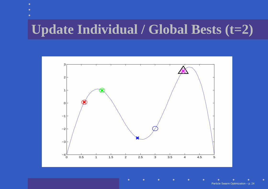
Update Individual / Global Bests (t=2)

0 0.5 1 1.5 2 2.5 3 3.5 4 4.5 5−4

−3

−2

−1

0

1

2

3


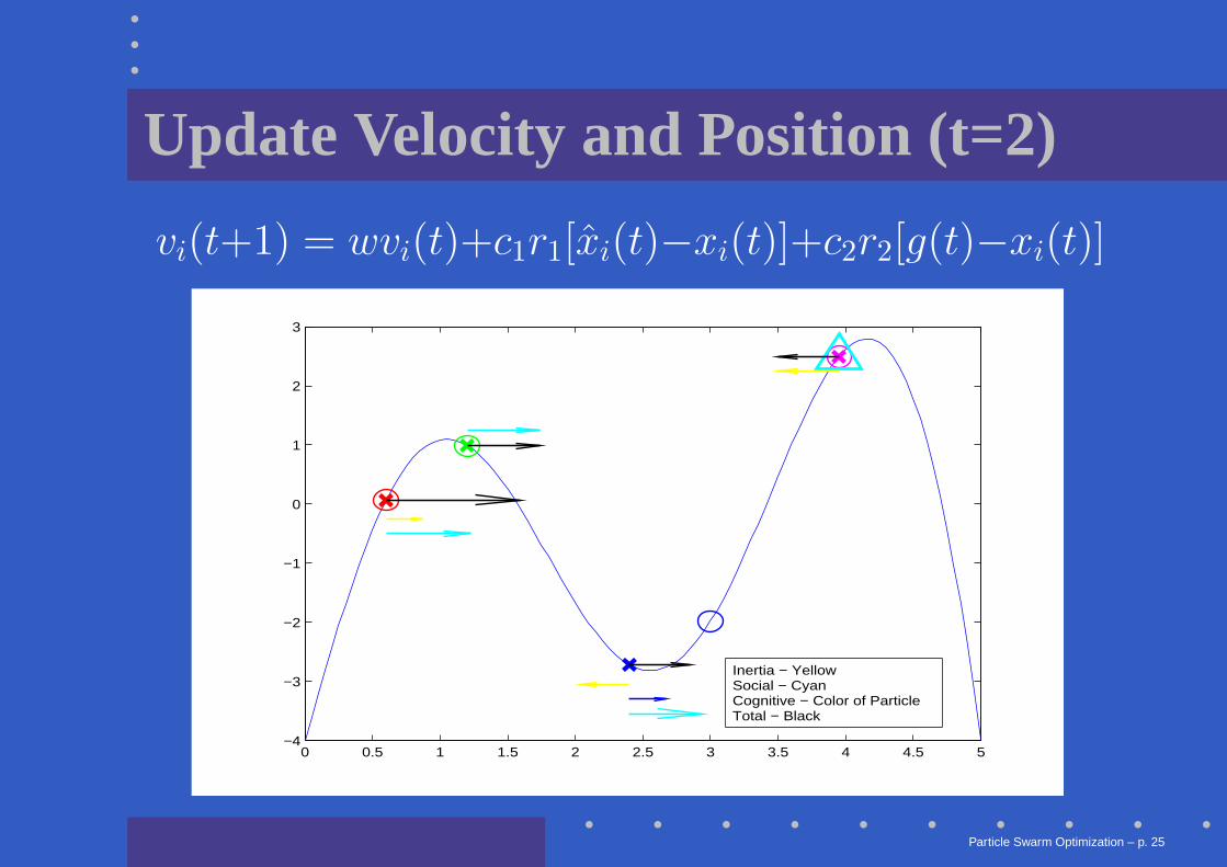
Update Velocity and Position (t=2)


0 0.5 1 1.5 2 2.5 3 3.5 4 4.5 5−4

−3

−2

−1

0

1

2

3

Inertia − YellowSocial − CyanCognitive − Color of ParticleTotal − Black


Classifier Optimization



Support Vector Machines

Support Vector Machines (SVMs) are a group ofmachine learning techniques used to classifydata.

• Effective at classifying even non-lineardatasets

• Slow to train• When being trained, they require the

specification of parameters which can greatlyenhance or impede the SVM’s effectiveness


Support Vector Machine Parameters

One specific type of SVM, a Cost-based SupportVector Classifier (C-SVC), requires twoparameters:

• Cost parameter (C), which is typicallyanywhere between 2−5 and 220

• Gamma parameter (γ), which is typicallyanywhere between 2−20 and 23


Supper Vector Machine Parameters

For different datasets, the optimal values forthese parameters can be very different, even onthe same type of C-SVC.

To find the optimal parameters, two approachesare often used:

• Random selection• Grid search


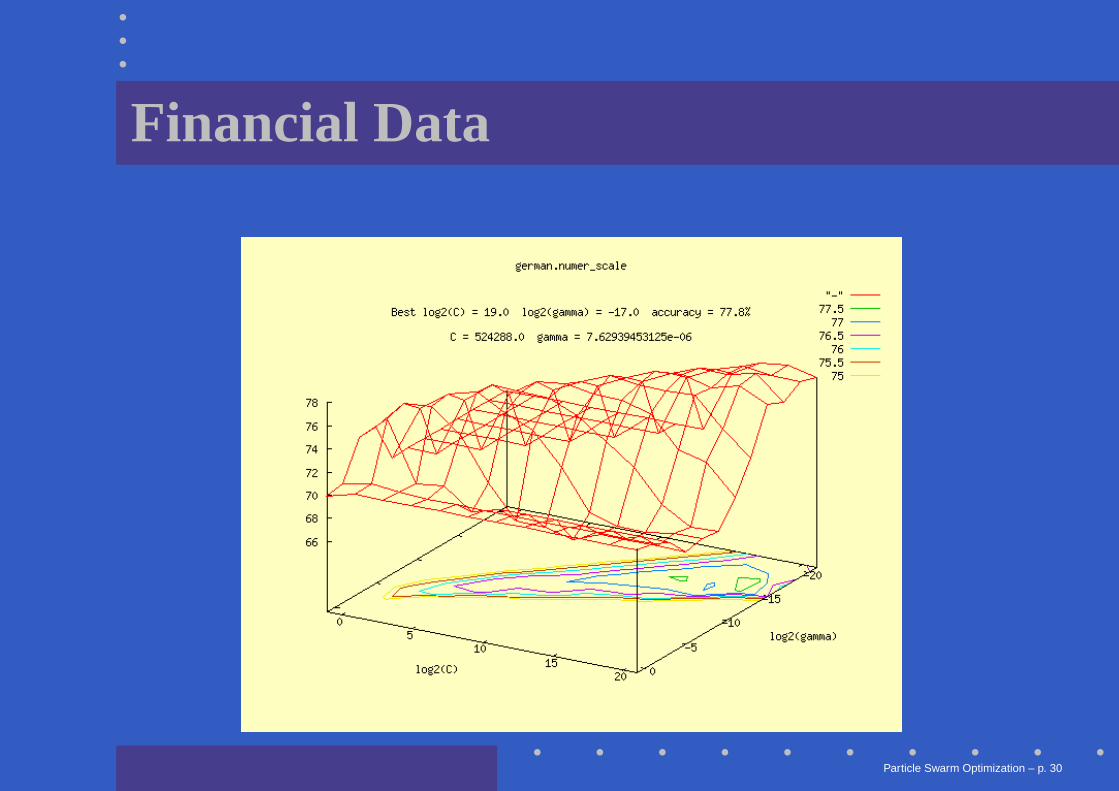
Financial Data


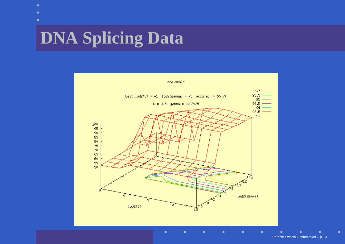
DNA Splicing Data


Grid Search Problems

While effective, grid search has some problems:

• Computationally intensive• Financial Data – 144 SVM training runs,

approximately 9 minutes• DNA Splicing Data - 110 SVM training

runs, approximately 48 minutes• Only as exact as the spacing of the grid

(coarseness of search), although once a peakhas been identified, it can be searched moreclosely


Applying PSO to SVM Parameters

Alternatively, PSO can be used to parameterizeSVMs, using the SVM training run as theobjective function.

Implementation considerations:• Finding maximum among two dimensions (as

opposed to just one, as in the example)• Parameters less than zero are invalid, so

position updates should not move parameterbelow zero


PSO Parameters

Parameters used for PSO algorithm:

• Number of particles: 8• Inertia coefficient (w): .75• Cognitive coefficient(c1): 1.8• Social coefficient(c2): 2• Number of iterations: 10 (or no improvement

for 4 consecutive iterations)


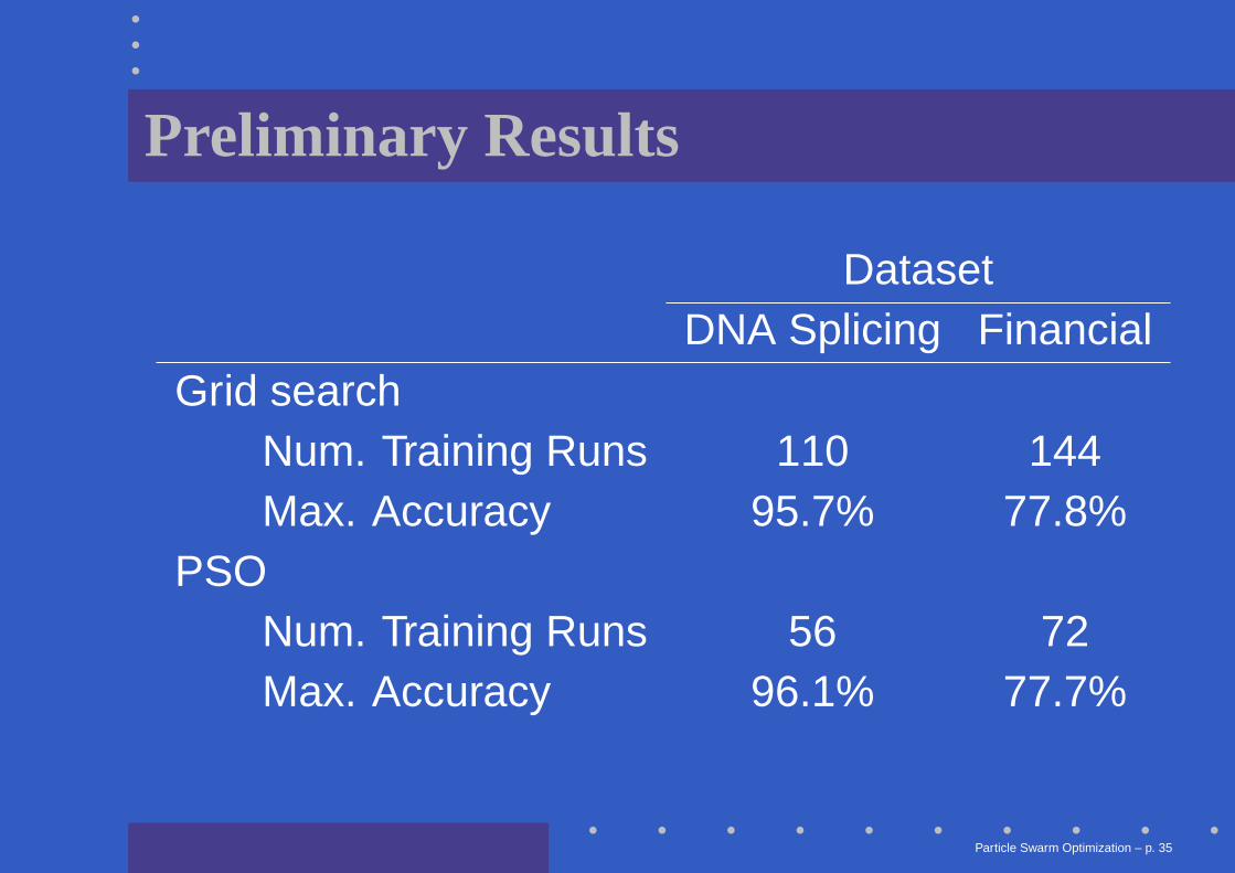
Preliminary Results

DatasetDNA Splicing Financial

Grid searchNum. Training Runs 110 144Max. Accuracy 95.7% 77.8%

PSONum. Training Runs 56 72Max. Accuracy 96.1% 77.7%


Analysis of Results

• Results are still preliminary, but encouraging• Due to randomized aspects of PSO

algorithm, the optimization process wouldneed to be run several times to determine ifresults are consistent

• Alternative PSO parameters can beattempted, and their effectiveness measured


Conclusion



Conclusions and Future Work

Conclusions:• Significant speedup using PSO over

exhaustive search• Additional testing needed

Future Work:• Other PSO variants can be tried• Need to find optimal parameters for PSO itself


Questions

Questions?


Documents

Particle Swarm Optimization - Georgia Southern … · Particle Swarm Optimization Applications in Parameterization of Classiﬁers James Blondin [email protected] Armstrong Atlantic