Partition function zeros for the two-dimensional Ising model VII

Physica A 154 (1989) 344-364

North-Holland, Amsterdam

PARTITION FUNCTION ZEROS

ISING MODEL VII*

John STEPHENSON

Physics Department, University of Alberta,

Received 1 July 1988

FOR THE TWO-DIMENSIONAL

Edmonton. Alberta. Canada, T6G 2Jl

The density of the complex temperature zeros of the partition function of the two-

dimensional Ising model on completely anisotropic triangular lattices is investigated near real

and complex critical points. The non-uniform behaviour of the density of zeros at interior and

boundary critical points is studied analytically, and numerically for a lattice with interactions

in the ratios 3:2: 1. The limiting behaviour of the density at complex critical points depends

on the direction of approach in the complex plane. In the neighbourhood of interior critical

points one finds only a single layer of zeros. But generally there are two layers or superposed

sets of zeros with different distributions, and different limiting densities at boundary critical

points. On anisotropic quadratic and on partially anisotropic triangular lattices the two layers

become identical, by symmetry of the partition function. The divergence of the (two-

dimensional) density of zeros at real critical points is discussed briefly in relation to scaling

theory.

1. Introduction

In this paper we study the complex temperature zeros of the partition

function of the two-dimensional king model on completely anisotropic triangu-

lar lattices by presenting some of the results of calculations of the density of the

zeros using a recently derived “exact” formula valid throughout the regions

containing zeros [l]. We shall confine our attention to the neighbourhood of

points which are solutions of the critical-point equations. The ferromagnetic

Curie point and the antiferromagnetic Neel point are given by the positive real

solutions, but there can also be complex solutions at which the distribution of

partition function zeros can have exotic behaviour. Complex solutions will be

called interior critical points if they lie inside the region containing zeros, and

critical pinch-points, or boundary critical points, if they occur where two

boundary lines meet.

* This work is supported in part by NSERC through grant #A65Y5.

0378-4371 i 89 lSO3.50 0 Elsevier Science Publishers B .V.

(North-Holland Physics Publishing Division)

.I. Stephenson I Partition function zeros for Ising model VII 345

Interior critical points cannot occur on anisotropic quadratic or on partially

anisotropic triangular lattices [2] (to be referred to as IV). It is therefore

necessary to study completely anisotropic triangular lattices. One can see from

fig. 2b in IV that the density of zeros for a (3,2,1) triangular lattice is quite

low near an interior critical point at R. We suggested in IV, on the basis of the

structure of the density formula, that the density might be zero at such points:

incorrectly as it turns out. However, the density of zeros does behave in a

peculiar fashion at interior critical points, since it can acquire different limiting

values, depending on the direction of approach in the complex plane, or in the

corresponding angle diagram.

Pinch-points occur wherever two boundary lines intersect. Critical pinch-

points are also solutions to the critical point equations, as are L and M on the

(3,2, 1) lattice. Pinch-points which lie on the unit circle occur for other

reasons, as explained in IV. Pinch-points were also noticed on a class of

quadratic lattices by Wood [3] and by Wood and Turnbull [4]. The non-uniform

behaviour of the density of zeros at critical pinch-points is complicated further

by the proximity of the two intersecting boundary lines on which the density is

infinite, and by the superposition or overlap of the two sets of zeros.

The density of zeros near the physical critical points - the Curie and NCel

points - is also complicated by the superposition of two sets of zeros and by the

fact that the boundary lines now meet at the real axis in a parabolic cusp.

Expressions for the density of zeros near real critical points have previously

been obtained for quadratic lattices by Stephenson and Couzens [5] (to be

referred to as I), and for triangular lattices by Stephenson [6] (to be referred to

as II). [See also W. van Saarloos and D.A. Kurtze [7].] These formulae can be

written in a scaled form [8], which reveals the non-uniform behaviour in more

detail.

The situation on anisotropic quadratic and on partially anisotropic triangular

lattices is expected to be much simpler, since the boundary criteria are

“trivial”, and one can immediately see evidence for mesh-lines in the figures

presented in earlier papers of this series: [9,2, lo] (to be referred to as III, IV,

V, respectively). So these lattices will be covered only briefly here.

We now investigate the behaviour of the density of zeros: numerically on a

lattice with interactions in the ratios 3: 2: 1, and analytically by obtaining

explicit expressions for the limiting values of the density of zeros at real and

complex critical points for a general direction of approach.

In sections 2-4 we summarize the basic formulae for the partition function

polynomials, the critical point equations, and the Jacobian expression which

determines the boundary. In section 5 we make some modifications to the

general formula for the density of zeros per lattice site so that it applies to each

branch or set of zeros at a point of the complex z-plane. In sections 6-9 we

346 J. Stephenson I Partition function zeros for king model VII

discuss zeros near and at interior critical points, obtaining a general expression

for the limiting density at any complex critical point. The density of zeros near

and at critical pinch-points is analyzed in section 10, and near real critical

points in section 11. The situation on anisotropic quadratic and on partially

anisotropic triangular lattices is discussed in section 12.

2. Partition function polynomials

The polynomial factors which determine the zeros of the partition function

of the Ising model on an anisotropic two-dimensional triangular lattice, with

interactions in the ratio a: b: c, have the form [2]

f(z; 4,, 4,) = g + ih = A + B COS 4,. + c COS 4, + D COs(4, + 4,) - (1)

where A, B, C, D are polynomials in z = x + iy = exp(-2J/k,T):

B = 2Zh+C(Z2ff ~ 1) = 2(z”+p _ zf) , W)

c = 2Z(~+yZ*~~ _ 1) = qzf+d _ f) , (24

D = 2Zu+‘1 (z2c _ 1) = qzr+l _ Zd) _ WI

withd=a+h,e=c+a,f=b+c.Laterwewillneedthez-derivativeof(l)

in the form:

f, = zf’(z; c$, , 4,) = A z + B, cos 4, + C; ~0s 4, + D; cos(d% + 4,s ) 1 (3)

where a subscript z denotes z times a derivative with respect to z. For a finite

m X II lattice the angles are

4, = (2r - 1)rrlm , r=l,...,m,

(4) 4,$ = (2s ~ l)?r/n ) s=l,...,n.

Since the large lattice limit is required, the angles will be treated as continuous

in the range O< $,, $I, <2~.

J. Stephenson / Partition function zeros for Ising model VII 347

3. Critical point equations

Many of the features of geometric interest in the distribution of zeros are

located by the solutions to the critical point equations which arise on setting 4,

and $S equal to 0 and/or n in (l), to obtain

at (0, 0) , l-zd-+Zf=(), (54

at CT, 0) , l+Zd-.?+zf=o, (5b)

at (0, ~1 , l+Zd+Ze-Zf=O, (5c)

at (T, 4 , l-Zd+_zC+Zf=O. (5d)

In all cases the Curie point is the real positive solution to (5a). Usually we

choose the interaction strengths so a > b > c. Then the NCel point is the real

positive solution to (5d). The non-physical solutions to these equations often

correspond to other features of interest, such as boundary “pinch-points” (see

IV), and the interior critical points to be discussed below. In table I we provide

(for convenient reference) a list of the special points on the (3,2, 1) lattice.

4. The boundaries of zeros

The boundaries of the region containing zeros are determined by the

vanishing of the Jacobian between g, h, the real and imaginary parts of

Table 1

Special points for the (3,2, 1) lattice: C is the Curie

point and N is the N&e1 point. R, L and M are critical

pinch-points. P and Q are pinch-points on the unit

circle. As in IV, D’ (J) locates the upper boundary and

I the lower boundary at the imaginary axis.

I exp(igi2)

J (D’) (iz,) il.465571

C 0.754878 (2,) L 0.428538 + iO.710201

M 0.780990 + i0.492496

N 1.704903 (2,) P exp(ini4)

Q exp(ia/6) R 0.877439 + i0.744862

z 4,

lines

” 90”

0” 180”

0”

180”

line line

180”

(15) 0”

0 180

180

180

0"

348 J. Stephenson I Partition function zeros for Ising model VII

f = g + ih, and the angles +,, +,,:

a( JiTl h) J(z; 4r3 4s) = q4,, 4J

= (B’C,, - B’C’) sin 4, sin 4s

+ sin(4, + 4,s)[(B’D” - F’D’) sin 4, - (C’D” - C”D’) sin 4,>] ,

(6)

where we have written B = B’ + iB”, etc. In order to determine the boundary,

one has to solve the boundary equation (6) simultaneously with eq. (1) for the

zeros, as in IV. Near critical points the boundary expression Jacobian J

approximately assumes a quadratic form in sin 4, and sin 4,. If this quadratic

form is positive definite in the vicinity of a complex critical point then the point

is inside the zero distribution, as is the case at R. If the quadratic form is

indefinite then the point is a critical pinch-point at the intersection of two

boundary lines, as at L and M.

5. The density of zeros

Asr-l,..., mands-l,..., n, the angles 4,, 4,, cover the range 0 < 4,, 4,r < 27~ over a square in the angle diagram. [Alternatively we can use the

range pn < 4,, 4.y < T, so the four quadrants around the origin are involved.]

Zeros occur in cells of size 2nim x 27rin in the 4,, 4,y diagram. The number of

zeros in A4, A4, is therefore mn A4, A4,/(2rr)*. In order to get the correct

contribution to the density of zeros at a point in the complex z-plane, we must

multiply by a factor of 2 because of the symmetry under simultaneous reversal

of the signs of both angles, and also divide by 2 because the product of factors

in (1) yields the square of the partition function [6] (II). However, as we shall

see below, in order to obtain the correct density at a fixed point z = x + iy for a

completely anisotropic triangular lattice, it may now be necessary to sum

distinct contributions from different sets (or branches) of zeros arising from

different (pairs of) angles. For anisotropic quadratic and partially anisotropic

triangular lattices there is a four-fold symmetry around the (angle) origin, so

for these lattices either one must multiply by 4 (for the four quadrants, oriented

“+” for a quadratic lattice and “X” for a partially anisotropic triangular

lattice, as we did in II) instead of by 2 as above, or one must sum over two

equivalent sets of zeros. The density of zeros in the complex z = x + iy plane,

per lattice site and per brunch, is then given by [6]


For the Ising triangular lattice the remaining Jacobian, in the denominator of

(7), is given explicitly by J as in eq. (6), and the derivative f’(z) in the

numerator is in eq. (3). So all the quantities in this form for the density of

zeros can be calculated directly, using eqs. (l)-(6).

6. Numerical density of zeros near interior critical points

In order to investigate the density of zeros near and at interior critical points,

we begin with the example of the point R on the (3,2, 1) completely

anisotropic triangular lattice. R: 0.877439 + i0.744862 is a solution of the

critical point equation (5b) obtained by setting 4, = n, $,Y = 0 in f in (l), with

d, e, f= 5, 4, 3. The distribution of zeros around R is illustrated in fig. la, as

calculated from (1) for 4, = MY’--185” (A$, = O.S’), +,Y = - lo”-lo” (A$,Y =

0.5”). The corresponding “mesh-lines”, which are contours of constant 4, and

$, , are plotted in fig. lb. The principal mesh-lines (a): 4, = T and (b): $s = 0

are respectively almost horizontal and vertical in the complex z-plane, whereas

the direction (c): 4, + 4,1 = IT is roughly diagonal from upper left to lower right,

as shown in fig. 2a. The density of zeros appears to be higher along the

mesh-lines than in the quadrants in between. The nature of the zero distribu-

tion around R is revealed by numerical evaluation of the density, using eq. (7),

along the directions (a), (b) and (c). Within a degree of R, the densities of

zeros along these directions range between about 0.57-0.60 along (a), and

0.74-0.87 along (b), and is about 0.13 along (c), as in table II, and as graphed

in fig. 2b. Also there are very few zeros in the lower left and upper right

quadrants, where the (low) density is around 0.26 to 0.33 (roughly). Numerical

extrapolation into R, using table II, reveals that the limiting values of the

density depend on the direction of approach, and are approximately 0.584,

0.800 and 0.130 along the lines (a), (b) and (c), respectively.

7. Analytical density of zeros near interior critical points

We now confirm the non-uniform behaviour, observed above, analytically

along the directions (a), (b) and (c), by obtaining explicit expressions for the

limiting values of the density of zeros at R. For example, along (c), using 4, as

parameter with 4, = n - 4,Y, the polynomial for the zeros (1) becomes

= (1+ Zd - ze + *f)* + 2(zd + l)(z’ - Zf)(l - cos &) .

(8)

350 J. Sfephenson I Par&ion function zeros for Ising n-&d I/II

0.820

0.780 .'.:/~"".,., ..:,"'. ; : : : .,.,: .,.. '. .:,:,,*.. . . '., ‘..T '_ '.., ..,A,

0.760- '. . . '.y '., . . .r.. '. ',' ',

., "., 'T,, " ",',','.: : : . .

0.820

Y

0.8OC

0.78C

0.76C

t

+

i

i ._

I I / I I I Y

0.810 0.850 0.890 0.930

Fig. 1. Distribution of zeros around the interior critical point at R: 0.877439. + i0.744862 on the (3, 2, 1) completely anisotropic triangular lattice, as calculated from (1) for 4, = 175”-180

(A& = OS”), 4, = -lo”-10” (A$< = 0.5”). Th e zeros are plotted as points in (a) and the corresponding “mesh-lines”, which are contours of constant 4, and I$,, are plotted in (b).

J. Stephenson I Partition function zeros for Ising model VII 351

0.850

Y

0.810

0.770

cl .730

0.690

0.650

2.0-

G

1 .6-

0.8-

’ \’ I I I

b a

I , I, b

I I 1

I.830 0.870 0.910 x

c

0.0 ,R

I I I I I

0.830 0.870 0.910 X

Fig. 2. (a) Shows the principal mesh-lines in the z-plane near the interior critical point R:

0.877439 + i0.744862. for the (3,2, 1) lattice. The lines a: 4, = 180” and b: C#I~ = 0” are almost

horizontal and vertical, respectively. The line c: 4, + C#J, = 180“ is roughly diagonal from upper left

to lower right. (b) Shows the (continuous) variation in density along these lines as a function of

x = Re z.

At R the first (squared) term in (8) vanishes. To calculate the density as in (7)

we need the derivative:

zf’(z; n - &) &) = 2(dzd - ez’ + fzf)( 1 + Zd - ZE + z’)

+ 2[dzd(z’ - z’) + (z” + l)(eze - fzf)]( 1 - cos 4,) .

(9)

On substituting from (8) for the factor (1 + zd - z’ + zf) in (9), it is clear that


Table II (3,2, 1): Density of zeros near R: Density of zeros along the (principal) lines a: #J, = 180” and b:

c$, = 0” and c: 4, + 4, = 180” through the interior critical point at R: 0.877439. + i0.744862

on the (3,2, 1) lattice.

4, 4, x Y Density x Y Density Mean

180 0 0.877 0.745

-0.5 0.875 0.745

-1 0.873 0.744

-2 0.868 0.743

-4 0.859 0.742

-6 0.850 0.740

-8 0.841 0.738

- 10 0.X32 0.737

180

180.5

181

182

184

186

188

190

0 0.877 0.745

0.X78 0.740

0.879 0.735

0.879 0.725

0.881 0.706

0.882 0.687

0.882 0.669

0.882 0.652

180 0 0.877 0.745

1X0.5 -0.5 0.879 0.744

181 -1 0.881 0.743

182 -2 0.884 0.740

184 -4 0.891 0.735

186 -6 0.897 0.730

18X -8 0.903 0.725

190 -10 0.90x 0.719

0.584 0.877

0.592 0.880

0.600 0.882 0.617 0.887 0.653 0.897 0.694 0.907 0.741 0.917

0.794 0.928

0.800 0.877 0.834 0.877 0.86X 0.876 0.944 0. X75 1.120 0.872

1.337 0.868

1.610 0.863 1.955 0.858

0.130 0.877

0.130 0.876 0.130 0.874

0.130 0.870

0.131 0.862

0.133 0.854

0.135 0.846 0. 138 0.837

0.745

0.745

0.746

0.746

0.748

0.749

0.750

0.751

0.745

0.750

0.755

0.765

0.785

0.806

0.827

0.849

0.745

0.746

0.747

0.749

0.753

0.756

0.759

0.761

0.584 0.584

0.577 0.584

0.569 0.585

0.555 0.586

0.529 0.591

0.506 0.600

0.485 0.613

0.466 0.630

0.800 0.800

0.769 0.801

0.739 0.804

0.683 0.813

0.585 0.852

0.504 0.920

0.436 I ,023

0.378 I.167

0.130 0.130

0.130 0.130

0.129 0.130

0.130 0.130

0.130 0.131

0.132 0.132

0.134 0.135

0.137 0.137

the first term in (9) is the larger one. So close to R we have approximately:

Izf’(z)12 = 41dzd - ezF +fzf121B - C/(1 - cos 4,). (10)

Also along (c) the Jacobian in the boundary equation (6) collapses to

J R(c) = IB’C”- B”C’J(1 + cos &)(l - cos 4,) (11)

When (10) and (11) are substituted in the density formula (7), the factors

(1 - cos 4,), which vanish at R, cancel explicitly, leaving a finite limiting value

for the density of zeros at R, when R is approached along the line (c):

G _ = IB- cIJdz”-ez’+f_z~2 R(L) 2pC” _ Bllc1~~~z~2 = o.129531 . . . ’ (12)


confirming the earlier numerical estimate. Similarly along the lines (a) and (b)

we have

G Ic - Dlldz” - eze ffzf12

R(a) = =0.584151 . . . 7

and

G IB + D(ldzd - eze +fZfl*

R(b) = *prD” _ B,,D’I)Tz12 = 0,8m30~ . . 9

(13)

(14)

again confirming the numerical estimates. This checks that the density is

continuous at R along different directions.

8. Density of zeros near interior critical points for an arbitrary

direction of approach

The non-uniform nature of the density of zeros at any interior critical point

with 4, = T, 4s = 0, such as R, can be determined for an arbitrary direction of

approach by extending the analytical method for general values of the angles

close to (180”, 0”). The result close to R is

G, = 21dzd - eze + fzf12

x IB(sin (CI,)’ + D(sin (cr, + sin J+!J~)’ - C(sin tJ~)*j lJI7rz(* ,

where

(15)

J = 4[a(sin tir)’ + p(sin *r sin (cl,) + y(sin +!J~)‘] ,

with

(16)

a = B’D”- B”D’ , y = C’D” - c”D’ ,

p = a + y - (B'," - B”,‘). (17)

Here z, A, B, C, D are evaluated at R, and we have introduced the angles

!&= %++ 9, = t G% (IS)

(for convenience), which are small around R. In the limiting density formula

(15) at R it is understood that I,!J~, $s -0 in such a way that non-uniform density of zeros at R can be parameterized by the (limiting) ratio

sin +!Jslsin +!I~ 2: +!J~I*~ = tan 9 , say , (19)

354 .I. Stephenson i Partition function zeros for lsing model VII

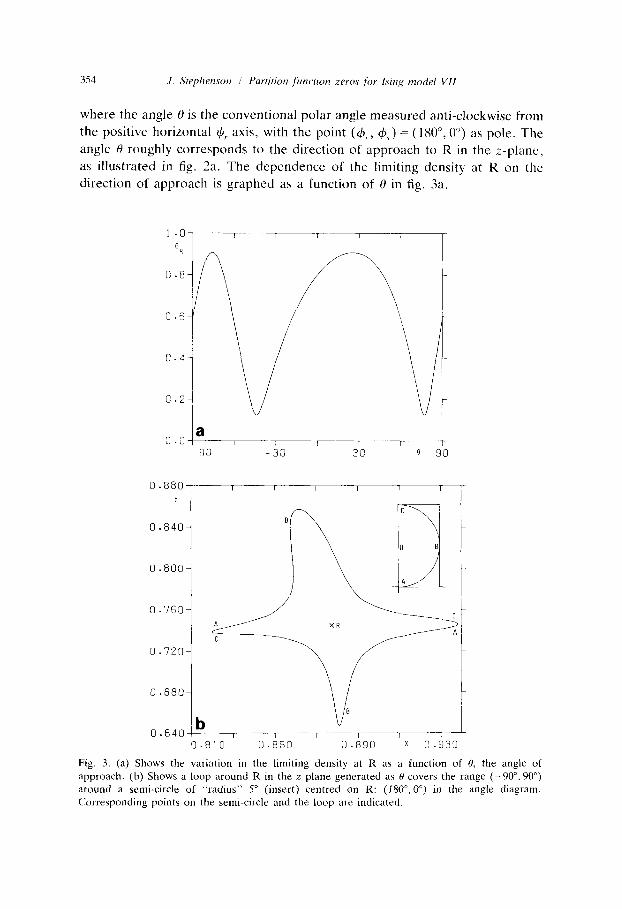
where the angle 0 is the conventional polar angle measured anti-clockwise from

the positive horizontal 1cI, axis, with the point (4,, 4,) = (180”, 0’) as pole. The

angle 0 roughly corresponds to the direction of approach to R in the z-plane,

as illustrated in fig. 2a. The dependence of the limiting density at R on the

direction of approach is graphed as a function of 0 in fig. 3a.

0.840

0.800

1

0.760-

0.720-

0.680-

I I

0.810 0.850 0.890 x 0.930

Fig. 3. (a) Shows the variation in the limiting density at R as a function of 0, the angle of

approach. (b) Shows a loop around R in the z-plane generated as 0 covers the range (-SW. 90”)

around a semi-circle of “radius” 5” (insert) centred on R: (IW, 0”) in the angle diagram.

Corresponding points on the semi-circle and the loop are indicated.


It is helpful for visual purposes and for technical reasons (later on at

pinch-points) to relate the non-uniform density variation both to the direction

of approach to R in the angle diagram as determined by (the ratios of) 4,) C/I,,

and to the corresponding direction(s) in the complex z-plane. In order to

achieve this, first trace a small semi-circle around the pole (ZSOO, 0”) on the

right-hand side where 4, > n, as 8 covers the range (-90”, 90”), by setting

1cI, = p cos 0 ) (cr, = p sin 0 , (20)

where p is a “small” radius in the angle diagram (e.g. about 5” or 1P). [A

semi-circle on the left-hand side merely duplicates things, because of symmetry

under sign reversal of both angles, and has already been taken into account by

a factor of 2 in the density as explained in section 5.1 One can then inspect the

corresponding “contour” in the z-plane, to determine its location, and the

direction(s) in which it is traced out as 0 varies. Such a contour is shown in fig.

3b for the (3,2, 1) lattice at R, with the associated semi-circle as an insert.

Interior critical points are completely surrounded by such a contour, with each

set of angles contributing zeros at (roughly) diametrically opposed locations

relative to the interior critical point in the z-plane, while the density varies

through one cycle.

On other completely anisotropic triangular lattices an analogous non-unifor-

mity of the density is expected to appear at any interior critical points which

may arise from solutions to any of eqs. (3). [For example the interior critical

points J and T on a (4,2, 1) triangular lattice satisfy (3a) and (3b), as discussed

in IV.] The required generalization of (1.5) is derived in the next section.

9. Density of zeros at general complex critical points

Our formula for the limiting non-uniform density at the interior critical point

R at (rr, 0) can easily be generalized so as to hold at any complex critical point,

by defining (cr,, I+!I~ appropriately, and by introducing factors r, s, t to account for

the values of $,, $,Y at the pole. Set

r = cos 4, , s = cos 4, ) t=cos(4,+ 4,) >

at the pole, so r = st, s = tr, t = rs, and r2 = s2 = t2 = 1. Then set

(21)

+Gr=i4, ifr=+l, or *r= ;(4,-T) if r=-1

and (22)

+!fs = i 4.r if s = + 1 , or I/J,=+(~,-n) ifs=-1.

356 .I. Stepherwm I Pariition function zeros for lsing model VII

The critical point equations (5) can now be combined into a single form:

rzd + SZB + tzf = 1 . (23)

Then it is elementary to prove that

lzfyz)l* = SItLiz” + sef + rfzfl’

x IrB(sin 4r)2 + sC(sin $,y)2 + tD(sin $, + sin ticlr)‘l (24)

and

J = 4{s{ BD}(sin $r)2 + y{ DC}(sin $Z)2

+ [t{BC} + s{BD} + Y{DC}] sin *r sin $,y} . (25)

The {. .} terms are defined (for abbreviation) by

{ BC} = (B’C” - B”,‘) , {BD} = (BID”_ B”,‘),

(26) {DC} = (D’P - DUC’)

The density of zeros follows on substitution in (7). The Jacobian J is just a

quadratic form in X = 2 sin $,, Y = 2 sin $, :

J = Q = CYX’ + PXY + y Y' = il[cu(sin Gr),)’ + p sin ICI, sin e5 + y(sin $,)‘I ,

(27) where

a = rt{ BD} , y=ts{DC}, p = CY + y + n(K). (28)

[(27) and (28) g eneralize (16) and (17) above. This quadratic form is essential-

ly the same as the one in eq. (17) in IV except that the signs of X and p are

opposite.] In terms of 0, as defined in (19), the limiting non-uniform density of

zeros per lattice site, and per branch, at any complex critical point is:

G = Itdz” + sez’ + rfz’J*IrB( cos 0)’ + tD(cos 8 + sin 0)’ + sC(sin o)‘I

2\-rrz~*]a(cos 0)’ + p cos 0 sin 0 + y(sin O)‘l

(29)

Numerical values of the 0 dependence of the limiting densities at the complex

critical points R, L and M on the (3,2, 1) lattice are given in table III. [The

(3,2, 1) lattice has critical pinch-points at L and M arising from solutions of the


Table III Limiting density of zeros at R, L, M: Values of the limiting density of zeros at the complex critical points R, L and M, on the (3,2, 1) lattice, for 0 in the range (-9P, 90”).

-90 0.584 0.850 32.863

-85 0.765 1.156 101.685 ~ 80 0.878 1.785 79.595 -75 0.906 2.994 26.214 - 70 0.850 6.269 14.432

-65 0.731 87.174 9.031

-60 0.573 7.908 5.751

-55 0.402 3.763 3.382 -50 0.241 2.406 1.441

-45 0.130 1.712 0.844 -40 0.164 1.291 2.953 -35 0.272 1.024 6.251 -30 0.380 0.869 13.386 -25 0.478 0.813 60.797 -20 0.563 0.842 30.284 -1.5 0.637 0.937 12.186 -10 0.701 1.083 7.295

-5 0.755 1.269 4.854 0 0.800 1.495 3.299

R L M 0 R L M

5 0.837 1.767 2.173 10 0.867 2.102 1.301 15 0.888 2.528 0.680 20 0.902 3.098 0.651 25 0.907 3.919 1.142 30 0.903 5.243 1.731 35 0.889 7.825 2.347 40 0.863 15.459 2.992 45 0.823 2272.442 3.679 50 0.766 14.330 4.432 55 0.690 6.836 5.281 60 0.591 4.270 6.273 65 0.467 2.939 7.481 70 0.316 2.104 9.030 75 0.159 1.520 11.152 80 0.170 1.102 14.351 85 0.369 0.850 19.943 90 0.584 0.850 32.863

critical equations (5~) and (5d) at ( r, IT) and (0, IT), respectively (see IV). For

the (3,2, 1) lattice these two equations transform into one-another under

z+ -z.]

10. Density of zeros near and at critical pinch-points

At critical pinch-points two boundary lines cross, so it is obvious that there

cannot be a closed contour around a pinch-point in the z-plane. However, the

limiting density formula (29) continues to give values for G for all values of 8

in the range (-90”, 90”) around a semi-circle in the angle diagram, as illus-

trated in fig. 4a for the critical pinch-point L on the (3,2, 1) lattice. Examina-

tion of the situation near (p = 5” in (20)) L reveals that there are now two

closed loops on diagonally opposite sides of the pinch-point, as illustrated in

fig. 4b. The loops touch both the boundary lines, so as one approaches L there

are contributions to the density of zeros from both the “nearer” and “further”

portions of each loop. As one traces out a semi-circle in the angle diagram, the

formula (29) gives two distinct limiting values for density at L, corresponding

to the nearer and the further sides of each loop. Moreover for a given pair of

angles, the limiting value of the density at L is closely approximated by the


40- I -- T G i a

3G-

0.800- Y

0.780-

0.760-

0.740-

0.720-

0.700-

0.680-

0.660-

0.640 j , , I I I I I I 0.370 0.430 x 0.490

Fig. 4. (a) Shows the variation in the limiting density at the critical pinch-point L: 0.428538. + iO.710201 on the (3.2, 1) lattice, as a function of 0, the angle of approach. (b) Shows the loops

generated in the z-plane as 0 covers the range (-9tY’. 90”) around semi-circles of radii 5” and IO”

centred on L: (180”, 180”) in the angle diagram. The loops he between the boundary lines in pairs

on opposite sides of the pinch-point.

mean of the densities at corresponding points on the loops on either side of L.

There is a similar behaviour near M.

One now sees that there is an overlap or superposition of two sets of zeros

on each side of a critical pinch-point: each point in the z-plane is intersected by

two loops. The complete correspondence between the densities and the angles

and the points in the z-plane for the loops can be extracted from the numerical

data in table IV. [The same range of 8 has been used in both tables III and IV.1

J. Stephenson I Partition function zeros for king model VII 350

Table IV Numerical data for the loops in the z-plane near the critical pinch-point L: 0.428538 + iO.710201 on the (3,2, 1) lattice. Values of the angles (c#J,, 4,), points z =x + iy, and the density of zeros, are tabulated as functions of 0 in the range (-9P, 90”) around a semi-circle of radius 5” centred on L: (180”, 180”) in the angle diagram.

4, x Y Density I J’ Density Mean At L

-90 180.000 170.000 0.4448 0.7043 0.863 0.4125 0.7170 0.838 0.850 0.850

-80 181.736 170.152 0.4504 0.7095 1.810 0.4079 0.7113 1.768 1.789 1.785

-70 183.420 170.603 0.4545 0.7115 6.444 0.4045 0.7092 6.132 6.288 6.269

~60 185.000 171.340 0.4565 0.7116 7.634 0.4030 0.7090 8.267 7.951 7.908

-SO 186.428 172.340 0.4564 0.7104 2.360 0.4032 0.7104 2.460 2.410 2.406

~40 187.660 173.572 0.4545 0.7076 1.264 0.4047 0.7136 1.314 1.289 1.291

-30 188.660 175.000 0.4515 0.7028 0.848 0.4071 0.7188 0.881 0.864 0.869

-20 189.397 176.580 0.4490 0.6964 0.820 0.4086 0.7259 0.855 0.837 0.842

- 10 189.848 178.264 0.4479 0.6899 1.058 0.4087 0.7329 1.110 1.084 I.083

0 190.000 180.000 0.4474 0.6846 1.465 0.4080 0.7386 1.552 1.509 1.495

10 189.848 181.736 0.4471 0.6807 2.062 0.4074 0.7429 2.219 2.140 2.102

20 189.397 183.420 0.4467 0.6783 3.025 0.4070 0.7455 3.345 3.185 3.098

30 188.660 185.000 0.4460 0.6773 5.036 0.4072 0.7466 5.925 5.481 5.243

40 1X7.660 186.428 0.4452 0.6777 13.530 0.4080 0.7459 22.233 17.881 15.459 50 186.428 187.660 0.4443 0.6796 17.180 0.4093 0.7437 11.455 14.317 14.330

60 185.000 188.660 0.4432 0.6831 4.557 0.4110 0.7398 3.997 4.277 4.270

70 183.420 189.397 0.4422 0.6883 2.190 0.4130 0.7340 2.036 2.113 2.104

80 181.736 189.848 0.4419 0.6955 1.131 0.4143 0.7262 1.080 1.106 1.102 90 180.000 190.000 0.4448 0.7043 0.863 0.4125 0.7170 0.839 0.851 0.850

11. Density of zeros near real critical points

At the physical critical points on the real axis, the boundary lines become

“vertical” and meet tangentially in a parabolic cusp. Again it is obvious that

there cannot be a single closed contour, and a behaviour similar to that at

critical pinch-points is to be expected. Calculation for the (3,2, 1) lattice

reveals a loop structure as anticipated, and superposition of two sets of zeros

occurs, as illustrated in fig. 5. The density of zeros, now given by eq. (22) in II,

can be written in a scaled form [S]. To ascertain the dependence of the limiting

density on the direction of approach in the angle diagram, write the basic

Jacobian expression in the density of zeros in (7) in the form

a(+,, 4,) _ a(&, 4) d(h> $2) d(X, Y) d(u, u)

a@> Y) - a(+,, $2) d(X, Y) a(& u) d(x, Y> . (30)

[We refer the reader to section 3 of II, where the notation and derivation of the

formulae are given in detail. Note that in II we wrote w = x + iy, whereas here

we have w = u + iv.] Here X, Y are the quadratic forms relating the real and


0.05

Y

0.04

0.03

0.02

0.0:

I /

a T- 0

B

I’ C

0.25

Y

0.2c

0.15

0.10

0.05

0.00

I-

I-

T

I 0 .oo&

0.754000 1 I /

0.756400 x

b ‘I

N

, ‘I .6.500 1.6800 x 1.7100

Fig. 5. (a) Shows the loops generated in the z-plane near the Curie point C: 0.754878 , as 0

covers the range (-90°, 90”) around semi-circles of radii 2.5”. 5” and 10” centred on C: (o”, 0”) in

the angle diagram. (b) Shows the loops generated in the z-plane near the N&e1 point N:

1.704903 . as 0 covers the range (-9P, 90”) around semi-circles of radii 5” and 10” centred on

N: (180”. 180”) in the angle diagram.

imaginary parts of the w-variable to the angles (@,, 4,) as in (Sa) and (8b) in

II, quoted in (32) below. (I/J,, I&) is the vector of angles associated with the

quadratic forms as in II (eq. (13)). A n d U, u are the real and imaginary parts of

the complex w-variable employed in II:

= x + iy and w = u + iv = (1 - z”)/(z’ + z’) . (31)

The quadratic forms referred to above are

where R,, and R,, are constant coefficients as defined in II (eq. (6)). In

diagonalized form, with 4 = HI,!J.

where h, , A, are the eigenvalues, as in II (eq. (12)). Now the determinants of


the first three Jacobians in (30) are

&t ‘(“’ “I = det H

a(&, vu ’ det ‘(XT ‘>

a(+,, +*I = 4@11C12(h, - A?) >

det a(x’ ‘) -zu -=

a(& u) ’

(34)

where det H is evaluated in II (eq. (17)) and II (eq. (25)). The final factor in

(30) is just the Jacobian of the transformation from z to w at the (ferromag-

netic) critical point where w = 1:

det a(~, u> dw * _=_ = I I I dzd + e.9’ + fi’ *

a@, Y) dz z(l-*d) ’ (35)

where we have used the critical point equation (5a) to simplify the result.

Finally u = fl is given in terms of the angles by (32b) or (33). So on collecting

the above formulae for the Jacobians for substitution in (7), we have an

expression for the density of zeros (per branch) near a real critical point:

2vdet H dw *

4.i-r2G = 4*,$*(A1 - h2) dz l-1 ’

so

[i,b: + &]“’ 1 dzd + me +fif 2

G = det H W,G*( A, - AZ) I 27rz(l - z”) .

(36)

(37)

The above expression involves only the angles $, , q!t2, which themselves depend

linearly on the angles $,, C& and 1cI,, $s used earlier in this paper. One should

recall that the boundaries are given by $, = 0 or I+!J* = 0. In a similar manner

one can show that the same formula is valid at the antiferromagnetic critical

point, where w = -1.

Note that if the ratio of the (small) angles is fixed so tan 0 = $s/Qr, then the

scaling variable Y/X is constant too [S]. As one approaches a real critical point

in the angle diagram in a direction 8, or along the corresponding scaling line

(Y/X constant) in the z-plane, the limiting form (37) for the density diverges

inversely as the (angle) “radius” p, and the “amplitude” of divergence is

direction dependent. The associated “integrated” density of zeros is propor-

tional to the imaginary part, y = Im z or u = Im w, of the complex variable, as

discussed previously elsewhere [8].

362 .I. Stephenson i Partition function zeros for Ising model VII

12. Density of zeros on anisotropic quadratic and partially anisotropic

triangular lattices

It remains to deal with the simpler cases of anisotropic quadratic and

partially anisotropic triangular lattices. Our general formulae for the density

close to critical pinch-points (29) and real critical points (37) are still valid.

However there arc no interior critical points on these lattices, since the

quadratic form Q above collapses to a single term, and cannot be positive

definite. Nevertheless it is advisable to check the structure of the zero

distributions near these singular points by evaluating the limiting density. The

results of pinch-points for some selected quadratic and triangular lattices are

presented in table V. [The density is quoted per brunch. evaluated from (29).

and there arc two equivalent branches.] The density of zeros is unbounded

when the direction of approach is aligned with one of the boundaries. This

occurs on quadratic lattices when +,- or 4, equals 0 or 7~. and on partially

anisotropic triangular lattices when c$,- = ? 4,. The boundaries correspond to

lines of symmetry in the angle diagram, and the densities in table V reflect this

symmetry, which obviously arises from the invariance of the partition function

factors in (1). This means that there is a double layer of zeros (everywhere) for

these lattices, and the superposition problem does not arise. The two layers

have the same distribution, and are accounted for by a factor of 4 (instead of 2)

in the calculation of the density at a fixed point in the z-plane, as previously

explained in section 5. The distribution of zeros for these lattices were

examined numerically in III and IV. On visual inspection of the figures in these

papers one notices that the distribution of zeros is much “cleaner” than in the

general case, and mesh-lines can be distinguished quite clearly.

13. Concluding remarks

In this paper we have studied the distribution and density of complex

temperature zeros of the partition function of the two-dimensional Ising model

on completely anisotropic triangular lattices near and at complex critical

points. The non-uniform behaviour of the density of zeros at interior critical

points and at critical pinch-points has been investigated analytically and

numerically for a triangular lattice with interactions in the ratios 3 : 2 : 1. We

have derived a general formula for the limiting density at any complex critical

point for an arbitrary direction of approach. We have also obtained an

analytical result for the angle (direction) dependence of the density near the

real critical points.

Furthermore, analysis of the distribution of zeros around critical pinch-points

J. Stephenson I Partition function zeros for lsing model VII 363

Table V Limiting density at pinch-points for triangular and quadratic lattices: Values of the limiting density (per branch) of zeros at pinch-points on some selected quadratic and triangular lattices for 0 in the range (-90°, 90”), computed from eq. (29).

Type: Angles: X: Y:

B

Triangular lattices

(1,2,2) (2,2,1) 180, 180 180, 180 0.578649 0.304877 0.652576 0.754529

(1, 1,3) (3,3,1) 180, 180 180, 180 0.691776 0.534118 0.478073 0.622950

Quadratic lattices

(2,1,0) (3,1,0) 0, 180 0, 180 0.419643 0.566121 0.606219 0.458822

-90 -85 - 80 -75 -70 -65 -60 -55 -50 -45 -40 -35 -30 ~25 -20 -15 - 10

-5 0 5

10 15 20 25 30 35 40 45 50 55 60 65 70 75 80 85 90

0.740 0.613 1.516 1.917 0.380 0.538 1.086 1.835 0.357 0.578 0.744 1.888 0.745 0.734 0.619 2.094 1.283 0.996 0.877 2.486 1.998 1.389 1.440 3.141 3.063 2.012 2.337 4.268 5.014 3.195 3.970 6.516

10.524 6.605 8.501 13.189

10.524 6.605 8.501 13.189 5.014 3.195 3.970 6.516 3.063 2.012 2.337 4.268 1.998 1.389 1.440 3.141 1.283 0.996 0.877 2.486 0.745 0.734 0.619 2.094 0.357 0.578 0.744 1.888 0.380 0.538 1.086 1.835 0.740 0.613 1.516 1.917 1.176 0.775 2.016 2.126 1.675 1.004 2.605 2.461 2.272 1.303 3.334 2.946 3.036 1.702 4.290 3.638 4.100 2.270 5.650 4.670 5.773 3.173 7.825 6.366 8.982 4.917 12.044 9.706

18.345 10.020 24.454 19.605

18.345 10.020 24,454 19.605 8.982 4.917 12.044 9.706 5.773 3.173 7.825 6.366 4.100 2.270 5.650 4.670 3.036 1.702 4.290 3.638 2.272 1.303 3.334 2.946 1.675 1.004 2.605 2.461 1.176 0.775 2.016 2.126 0.740 0.613 1.516 1.917

6.436 5.704 3.104 2.732 1.941 1.691 1.319 1.138 0.913 0.793 0.616 0.583 0.394 0.505

0.266 0.561 0.309 0.714 0.477 0.929 0.703 1.200 0.982 1.542 1.339 1.995 1.835 2.639 2.609 3.668 4.084 5.660 8.371 11.507

8.371 11.507 4.084 5.660 2.609 3.668 1.835 2.639 1.339 1.995 0.982 1.542 0.703 1.200 0.477 0.929 0.309 0.714 0.266 0.561 0.394 0.505 0.616 0.583 0.913 0.793 1.319 1.138 1.941 1.691 3.104 2.732 6.436 5.704

364 .I. Stephenson I Partition function zeros for Ising model VII

and real critical points has revealed an overlapping or superposition of two sets

of zeros, whereas no such doubling occurred at interior critical points. This

means that some parts of the region containing zeros have a double layer of

zeros. The occurrence of double (or multiple) layers of zeros means that the

formula for the density of zeros must be applied to both (or all) sets of zeros

which may be present at any point of the complex z-plane. Moreover, there

must be some sort of division or (interior) boundary line between regions with

single and double layers.

The knowledge we have acquired on the nature of the distribution and

density of zeros near real and complex critical points provides us with a basis

on which to tackle the question of the global distribution throughout the

regions of the complex plane containing partition function zeros.

Acknowledgement

I would like to thank Dr. Radha Gourishankar for her assistance in

preparing the figures.

References

[l] .I. Stephenson, J. Phys. A: Math. Gen. 20 (1987) L331.

[2] J. Stephenson, Physica A 148 (1988) X8-106, to be referred to as IV.

[3] D.W. Wood, J. Phys. A 18 (1985) L481.

[4] D.W. Wood and R.W. Turnbull, J. Phys. A 19 (1986) 2611.

[S] J. Stephenson and R. Couzens, Physica A 129 (1984) 201-210. to be referred to as 1.

[6] .I. Stephenson. Physica A 136 (1986) 147-159, to be referred to as II.

[7] W. van Saarloos and D.A. Kurtze, J. Phys. A 17 (1984) 1301.

[B] J. Stephenson, J. Phys. A: Math. Gen. 20 (1987) 4513.

[9] J. Stephenson and J. van Aalst, Physica A 136 (1986) 160-175, to be referred to as 111.

[lo] J. Stephenson, Physica A 148 (1988) 107-123, to be referred to as V.

Documents

Partition function zeros for the two-dimensional Ising model VII