Embed Size (px)
Citation preview
Passivation Theory and itsApplication to Automotive Systems
Technical Report of the ISIS Groupat the University of Notre Dame
ISIS-15-001March 2015
Meng Xia1, Arash Rahnama1, Shige Wang2 and Panos Antsaklis1
1Department of Electrical EngineeringUniversity of Notre DameNotre Dame, IN 465562General Motors R&D,
Warren, MI 48090
Interdisciplinary Studies in Intelligent Systems
The support of the National Science Foundation under Grant No.CNS-1035655 is gratefully acknowledged.
Passivation Theory and its Application to Automotive Systems
A Draft
M. Xia, A. Rahnama, S. Wang and P. J. Antsaklis ∗
March 12, 2015
Abstract
In this report, we consider a passivation method that uses an input-output transformationmatrix. This matrix generalizes the commonly used methods of series, feedback and parallel(or feedforward) interconnections to passivate a system. Through an appropriate design of thismatrix, positive passivity levels can be guaranteed for the system. The passivation parameterscan be selected by solving an optimization problem such as minimizing the tracking error. Asan application of our passivation method, we consider systems with input-output time delay.In automotive systems, time-delays cannot be avoided due to software implementations of thecontrol algorithms. We show that our passivation method can be used to compensate for thetime-delay in the controller and improve the closed-loop system performance. To validate ourresults, we provide simulation results in CarSim and Simulink.
1 Introduction
1.1 Cyber-physical Systems
Modern technology has undoubtedly penetrated the fabric of daily lives in advanced countries. Astechnology substitutes manual labor, the need for designing smart systems that help us performcertain daily tasks has increased. Consequently, the interconnection amongst these units becomesimportant as well. Hence it is important to come up with compositional systems that governthese interconnections such that each unit can perform as expected, and without the fear of anyintervention that might disrupt the system. This increased reliance on technological advancementaccompanied with new advancements in sensing, communications, control and computation havecreated an emerging class of complex systems called Cyber-physical Systems.
Cyber-physical Systems (CPS) consist of large number of complex yet closely interconnected andintegrated units. Examples of CPS may be found in smart transportation systems, smart medical
∗Xia, Rhanama and Antsaklis are with the Department of Electrical Engineering, University of Notre Dame,Notre Dame, IN 46556, USA (e-mail: {mxia, arahnama, antsaklis.1} @nd.edu). Wang is with General Motors R&D,Warren, MI 48090, USA (e-mail: [email protected]). The support of the National Science Foundation under theCPS Grant No. CNS-1035655 is gratefully acknowledged.
1
devices, and smart energy systems [1]. Loosely speaking, such systems consist of two primary units:the physical part, which provides the system with a continuous model of the physical world, usingordinary differential equations, and a communication and computational part, which monitors,coordinates, and controls the physical systems. The computational unit includes the softwarecomponent of the design and requires strong communication links in order to both receive andtransfer the data to the physical world [2]. The control of cyber-physical systems presents hugechallenges, so does the concern for maintaining their robustness, reliability and security issues.The concepts of dissipativity and, more specifically, passivity based on energy consumption of adynamic system provide a powerful tool for meeting the challenges that compositional systemsproduce. Passive systems do not generate energy, but only store or release the energy, which wasprovided to them. Under right conditions, passivity can present asymptotic stability for zero statedetectable (ZSD) systems [3]. Additionally, both negative feedback and parallel interconnectionsof passive systems stay passive, which means passivity and stability are preserved for large-scalesystems consisting of passive stable units [4]. This renders passive designs a suitable candidate fordesigning cyber-physical systems.
Our work was built upon the premise that an automobile meets all the criteria for a cyber-physical system. An automobile provides a platform consisting of both physical and computationalcomponents, both integrated through communication networks. Due to lack of a clear understand-ing of the complex and tight interactions that results from the integration of different controlcomponents, the design of automotive control applications is a complicated problem. The mainissue is that most problems with control applications occur in the final stages of the developmentcycle and correcting these mistakes at this level is both expensive and involves the modification ofthe design and requirements. As a result, the current common design approach relies on ad-hoctechniques with the goal of reaching the desire outcome through trial and error, which is not areliable approach. Passivity has been studied as a possible systematic solution to this problem.This approach is beneficial in regards to improving overall system performance, and potentiallycan help solve the scalability challenges given the increasing integration of more and more controlfunctionalities in vehicles.
1.2 Adaptive Cruise Control for Automotive Systems
The main function of the Adaptive Cruise Control (ACC) is to maintain the desired velocity set bythe driver. The ACC needs to adjust its speed based on the desired speed of the vehicle, the speedof the lead vehicle, and the distance between the two cars (the safety component of the design).This means that our system will have a hybrid structure of two modes, one to control vehicle whenit is accelerating, and one for when it is decelerating. Passivity has been studied extensively in thefield of control design and analysis as a suitable alternative to other nonlinear control techniques[5, 6]. And passivity conditions for hybrid and switched systems are discussed in [6, 7].
The design of the adaptive cruise control (ACC) has been extensively studied, and there arenumerous design techniques for deriving the corresponding control laws. Multiple-surface slidingcontrol containing a sliding control, and a switching rule between brake or throttle control wasused in [8, 9] which results in a smooth alternation between both controllers by solely relying onthe vehicle state and avoiding high frequency oscillation and risk of competing control inputs. Thisideal is reached by isolating the upper controller from the switching rule. Optimal control was
2
used in [10, 11] to design an ACC, and the performance was compared with that of the humandriver models. The results are that the performance is much smoother with a faster and bettertransient response. However, lack of well-defined safety features and due to time delay of theswitching rule, specifically for situations involving front cut-in vehicles, lead in collisions in someof the experiments under this design.[12] compares Fuzzy logic and H-infinity approaches for ACC.Overall the performances are slow in these designs, and Fuzzy logic design spends a considerabletime performing under the desired velocity. Neural networks, and proportional derivative (PD)type control laws were used in [13, 14].
Model based control for an implementation of an intelligent cruise control was examined in [15].This design performs well and the vehicle speeds match well in performed experiments. Raza andIoannou in [16] presented a high-level supervisory control design for vehicle longitudinal control.This supervisory controller processes the inputs from the driver, the infrastructure, other vehicles,and the onboard sensors and sends the appropriate commands to the brake and throttle control. [17]uses optimal dynamic back-stepping control to derive the desired acceleration on the supervisorylevel. However, most supervisory controllers are based on mathematical models rather than realhuman behavior. Closer to our work, human behavior is modeled through fuzzy controllers orneuro-controllers for spacing adjustments [18, 19]. Very similar to the idea of passivity, Druzhininaet al. [20] have designed an adaptive cruise control using a Lyapunov function approach. Passivity-based control to hybrid systems under the assumptions that the energy in each mode of the systemmust be bounded and that the composite energy of all modes (active or inactive) must also staybounded [21].
1.3 Systems with Input-output Delay
A time delay is defined as the time difference between the moment a control signal is applied andan observable change in the measured output that is the result of the applied signal [22]. Examplesof time delays in dynamical systems are computational delays, input delays, and measurementdelays. In addition higher order systems can be modeled by low order systems plus a time delay.Delays may introduce poor performance or instability to the closed loop system. In 1950s, OttoSmith introduced a unique predictive control method called the Smith Predictor that compensatesfor delay outputs using input values stored over a certain time window, and estimating the plantoutput accordingly [23]. Later this method combined with finite time integrals of the delayedinput values was expanded to include unstable plants as well. Accordingly, other control methodsfor handling time-delayed systems were developed [24]. Adaptive control may be used to controltime-delayed systems as well [25, 26]. In adaptive control, the structure of the controller is selecteddeductively, usually PD or PID. Ortega and Lozano introduced a control version of delay systems,which is capable of handling the uncertainty and accumulated error that is usually the result ofpredictive control methodologies for time-delayed systems [27]. Many examples of systems includingtime delays in chemical, biological, mechanical, and electrical systems are given in [28, 29]. A moredetailed survey of time delay systems can be found in [30, 31].
The driver control’s influence, and the vehicle and driver closed-loop systems have been inves-tigated by many authors [32, 33, 34]. In a vehicle and driver closed-loop system, the motion ofthe vehicle is usually described by a set of first-order differential equations where the response ofthe driver combined with a time-delayed human reaction appears as a break-throttle or steering
3
input term. The driver’s action is analyzed by observing the vehicle’s deviations with respect tothe desired states [32, 34, 35]. The effects of delay due to driver’s reaction has been analyzed forcar-following models [36, 37]. A small sum of delays that is less than 0.2 seconds does not play anessential role in the optimal velocity control according to [38]. However, for large delays, and sincethe acceleration of the vehicle depends on its velocity and distance from the preceding and frontvehicles, this large delay between the control decision and its exertion becomes problematic. Thismotivates a large field of research work, some mentioned in [39, 40, 41] and including our workpresented in this report that try to address and offer solutions for the problem.
1.4 Summary of Contributions
This report is motivated from the time-delay in automotive systems. As we discussed earlier, thetime delay may be due to signal processing delay, sensor measurement delay, or may be due tointeractions between different control algorithms implemented in the vehicle. Since the controlalgorithm is often designed by assuming that the time delay is zero, the presence of time delay maycause system instability and performance degradation. Thus, a method that can compensate forthe time delay is desirable. On the other hand, passivity and passivity-based control has showngreat promise in the control design of automotive systems. This is due to many properties thatpassivity can provide, such as stability, compositionality and robustness.
In the present report, our objective is to guarantee passivity of controllers with time delay.Since the passivation parameters can be used to tune the passivity indices of the controller afterpassivation, the passivated controller can be used to stabilize or passivate another plant. Further,we consider the passivation method that also optimizes system performance, such as minimizing thetracking error. Beyond guaranteeing passivity, desired system performance can also be achieved. Inorder to solve the optimization problem, we consider a co-simulation framework and non-derivativeoptimization method such that detailed modeling of the plant is not needed. Moreover, our pas-sivation method can be accommodated in order to consider other performance criteria, such asbeing a low pass filter by using transfer functions in the passivation method. Finally, simulationresults in CarSim and Simulink are provided to validate our theory, where a random time delaywas considered and a variety of reference inputs were tested.
It is worth mentioning that passivity itself can be viewed as a system performance criterionsince it can guarantee not only stability but also robustness with respect to modeling uncertainties[42, 43]. Under certain conditions, an optimal linear-quadratic-Gaussian (LQG) controller is strictlypositive real, thus the controller itself is guaranteed to be stable [44]. Design of strictly positivereal controllers using numerical optimization is considered in [45], where the objective functionis given by minimizing the closed-loop H2 norm. Optimality and passivity for nonlinear systemshave been studied in [46, 47], where optimality and passivity (with respect to a certain output)are shown to be equivalent. The passivity indices have been used to find optimal model predictivecontrollers in [48], where the model of the system can be inaccurate. In the present report, bytuning the passivation parameters, system performance such as minimizing the tracking error canbe achieved. Although mathematical relations between the performance and the passivity indiceswere not given, our setup in the co-simulation framework using non-derivative optimization methodprovide an ‘indirect’ manner to study the relation between performance and passivity.
The rest of the report is organized as follows. In Section 2, we provide a brief review of
4
passivity and dissipativity theory. The passivation method using constant parameters and transferfunctions is presented in Section 3. The optimization problem to find the passivation parameters isformulated in 4. Simulation results to illustrate the effectiveness of the passivation method throughCarSim/Simulink are presented in Section 5. Section 6 concludes the report.
Notation: The signal space under consideration is either the standard L2 space or the extendedL2 space. The exact space will be clear from the context. We use H : u→ y (or simply H) todenote a dynamical system with input u and output y. We use the notations u(t) and u for asignal interchangeably. We use G(s) to denote the transfer function for a SISO linear system. Then-dimensional identity matrix is denoted by In×n or simply I by omitting the dimensions if clearfrom the context.
2 Background on Passivity Theory
Consider a dynamical system given by an operator H : u → y, where u ∈ U denotes the inputand y ∈ Y denotes the corresponding output, and a real-valued function w(u, y) defined on U ×Y,called supply rate [49]. We assume that
∫ t1t0|w(u, y)|dt <∞, for any t0, t1 and any input u ∈ U .
Definition 1. An operator H : u → y is said to be dissipative with respect to supply rate w(u, y),if ∫ t1
t0
w(u, y)dt ≥ 0, (1)
for all t1 ≥ t0, and all u ∈ U . �
In particular, we can define passivity and L2 stability when the supply rate is in particularforms.
Definition 2. Suppose the system H : u → y is dissipative. It is said to be
• passive if w(u, y) = uT y;
• input feedforward passive (IFP) if there exists a constant ν so that w(u, y) = uT y − νuTu;we call such a ν an IFP level, denoted as IFP(ν);
• output feedback passive (OFP) if there exists a constant ρ so that w(u, y) = uT y− ρyT y; wecall such a ρ an OFP level, denoted as OFP(ρ);
• input-feedforward-output-feedback passive (IF-OFP) if there exist constants δ and ε so thatw(u, y) = uT y − δyT y − εuTu; we call such δ and ε passivity levels, denoted as IF-OFP(ε, δ);
• finite-gain L2 stable if there exists a constant γ 6= 0 so that w(u, y) = γ2uTu− yT y, denotedas FGS(γ).
Further, if ν > 0, then the system is said to be input strictly passive (ISP); if ρ > 0, then thesystem is said to be output strictly passive (OSP). Similarly, if δ > 0 and ε > 0, then the systemis said to be very strictly passive (VSP). The largest IFP level ν is called the IFP index and thelargest OFP level ρ is called the OFP index, respectively. �
5
yu)(sG
I
0u 0y
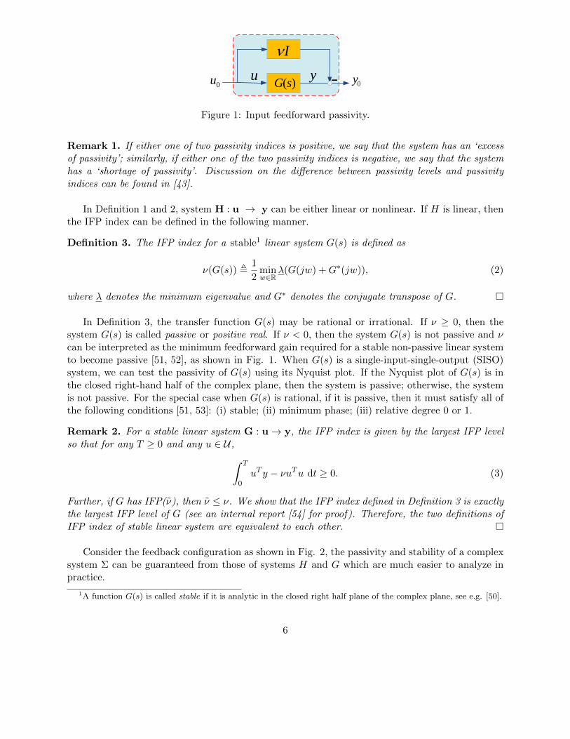
Figure 1: Input feedforward passivity.
Remark 1. If either one of two passivity indices is positive, we say that the system has an ‘excessof passivity’; similarly, if either one of the two passivity indices is negative, we say that the systemhas a ‘shortage of passivity’. Discussion on the difference between passivity levels and passivityindices can be found in [43].
In Definition 1 and 2, system H : u → y can be either linear or nonlinear. If H is linear, thenthe IFP index can be defined in the following manner.
Definition 3. The IFP index for a stable1 linear system G(s) is defined as
ν(G(s)) ,1
2minw∈R
λ(G(jw) +G∗(jw)), (2)
where λ denotes the minimum eigenvalue and G∗ denotes the conjugate transpose of G. �
In Definition 3, the transfer function G(s) may be rational or irrational. If ν ≥ 0, then thesystem G(s) is called passive or positive real. If ν < 0, then the system G(s) is not passive and νcan be interpreted as the minimum feedforward gain required for a stable non-passive linear systemto become passive [51, 52], as shown in Fig. 1. When G(s) is a single-input-single-output (SISO)system, we can test the passivity of G(s) using its Nyquist plot. If the Nyquist plot of G(s) is inthe closed right-hand half of the complex plane, then the system is passive; otherwise, the systemis not passive. For the special case when G(s) is rational, if it is passive, then it must satisfy all ofthe following conditions [51, 53]: (i) stable; (ii) minimum phase; (iii) relative degree 0 or 1.
Remark 2. For a stable linear system G : u→ y, the IFP index is given by the largest IFP levelso that for any T ≥ 0 and any u ∈ U ,∫ T
0uT y − νuTu dt ≥ 0. (3)
Further, if G has IFP(ν), then ν ≤ ν. We show that the IFP index defined in Definition 3 is exactlythe largest IFP level of G (see an internal report [54] for proof). Therefore, the two definitions ofIFP index of stable linear system are equivalent to each other. �
Consider the feedback configuration as shown in Fig. 2, the passivity and stability of a complexsystem Σ can be guaranteed from those of systems H and G which are much easier to analyze inpractice.
1A function G(s) is called stable if it is analytic in the closed right half plane of the complex plane, see e.g. [50].
6
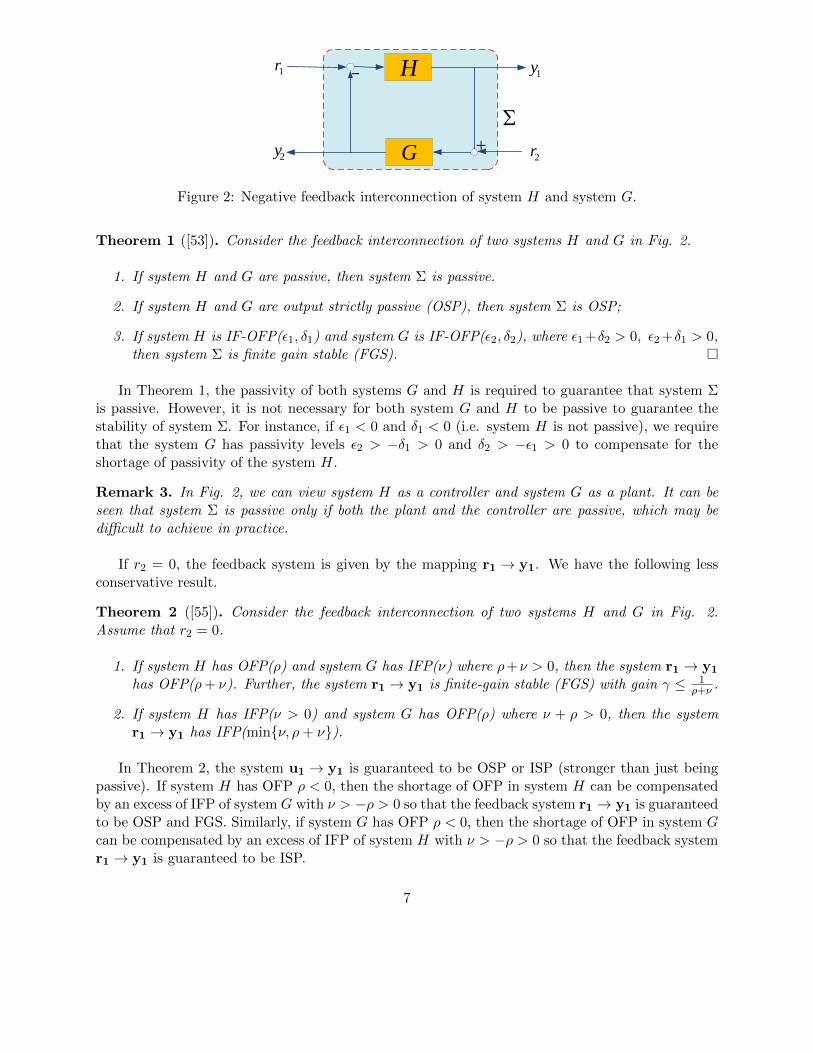
1y1r H
G
2y
2r
Figure 2: Negative feedback interconnection of system H and system G.
Theorem 1 ([53]). Consider the feedback interconnection of two systems H and G in Fig. 2.
1. If system H and G are passive, then system Σ is passive.
2. If system H and G are output strictly passive (OSP), then system Σ is OSP;
3. If system H is IF-OFP(ε1, δ1) and system G is IF-OFP(ε2, δ2), where ε1+δ2 > 0, ε2+δ1 > 0,then system Σ is finite gain stable (FGS). �
In Theorem 1, the passivity of both systems G and H is required to guarantee that system Σis passive. However, it is not necessary for both system G and H to be passive to guarantee thestability of system Σ. For instance, if ε1 < 0 and δ1 < 0 (i.e. system H is not passive), we requirethat the system G has passivity levels ε2 > −δ1 > 0 and δ2 > −ε1 > 0 to compensate for theshortage of passivity of the system H.
Remark 3. In Fig. 2, we can view system H as a controller and system G as a plant. It can beseen that system Σ is passive only if both the plant and the controller are passive, which may bedifficult to achieve in practice.
If r2 = 0, the feedback system is given by the mapping r1 → y1. We have the following lessconservative result.
Theorem 2 ([55]). Consider the feedback interconnection of two systems H and G in Fig. 2.Assume that r2 = 0.
1. If system H has OFP(ρ) and system G has IFP(ν) where ρ+ν > 0, then the system r1 → y1
has OFP(ρ+ ν). Further, the system r1 → y1 is finite-gain stable (FGS) with gain γ ≤ 1ρ+ν .
2. If system H has IFP(ν > 0) and system G has OFP(ρ) where ν + ρ > 0, then the systemr1 → y1 has IFP(min{ν, ρ+ ν}).
In Theorem 2, the system u1 → y1 is guaranteed to be OSP or ISP (stronger than just beingpassive). If system H has OFP ρ < 0, then the shortage of OFP in system H can be compensatedby an excess of IFP of system G with ν > −ρ > 0 so that the feedback system r1 → y1 is guaranteedto be OSP and FGS. Similarly, if system G has OFP ρ < 0, then the shortage of OFP in system Gcan be compensated by an excess of IFP of system H with ν > −ρ > 0 so that the feedback systemr1 → y1 is guaranteed to be ISP.
7
3 Passivation Results
3.1 Passivation Using Constant Parameters
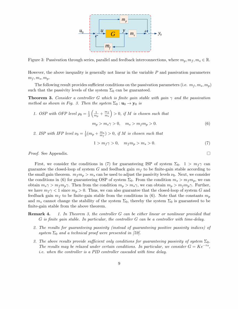
Many methods are known for passivation of non-passive systems, such as series, feedback, parallelor a combination of such schemes [51, 56, 57, 58]. These passivation mechanisms require the systemto satisfy certain properties, such as constraints on the relative degree, stability or minimum-phaseproperty of the system. For instance, feedback passivation can only be applied to systems thatare of minimum phase and have relative degree less than or equal to one [51]. For systems ofthe form G0(s)e
−τs, by using Pade approximations, we know that such systems are approximatelynon-minimum phase and thus they cannot be passivated through feedback alone.
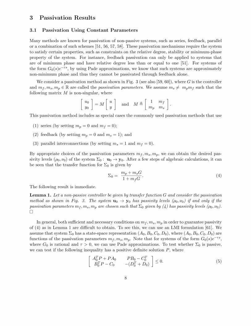
We consider a passivation method as shown in Fig. 3 (see also [59, 60]), where G is the controllerand mf ,ms,mp ∈ R are called the passivation parameters. We assume ms 6= mpmf such that thefollowing matrix M is non-singular, where[
u0y0
]= M
[uy
]and M ,
[1 mf
mp ms
].
This passivation method includes as special cases the commonly used passivation methods that use
(1) series (by setting mp = 0 and mf = 0);
(2) feedback (by setting mp = 0 and ms = 1); and
(3) parallel interconnections (by setting ms = 1 and mf = 0).
By appropriate choices of the passivation parameters mf ,ms,mp, we can obtain the desired pas-sivity levels (ρ0, ν0) of the system Σ0 : u0 → y0. After a few steps of algebraic calculations, it canbe seen that the transfer function for Σ0 is given by
Σ0 =mp +msG
1 +mfG. (4)
The following result is immediate.
Lemma 1. Let a non-passive controller be given by transfer function G and consider the passivationmethod as shown in Fig. 3. The system u0 → y0 has passivity levels (ρ0, ν0) if and only if thepassivation parameters mf ,ms,mp are chosen such that Σ0 given by (4) has passivity levels (ρ0, ν0).�
In general, both sufficient and necessary conditions onmf ,ms,mp in order to guarantee passivityof (4) as in Lemma 1 are difficult to obtain. To see this, we can use an LMI formulation [61]. Weassume that system Σ0 has a state-space representation (A0, B0, C0, D0), where (A0, B0, C0, D0) arefunctions of the passivation parameters mf ,ms,mp. Note that for systems of the form G0(s)e
−τs,where G0 is rational and τ > 0, we can use Pade approximations. To test whether Σ0 is passive,we can test if the following inequality has a positive definite solution P , where[
AT0 P + PA0 PB0 − CT0BT
0 P − C0 −(DT0 +D0)
]≤ 0. (5)
8
Gyu
0y0u
pm
sm
fm
Figure 3: Passivation through series, parallel and feedback interconnections, where mp,mf ,ms ∈ R.
However, the above inequality is generally not linear in the variable P and passivation parametersmf ,ms,mp.
The following result provides sufficient conditions on the passivation parameters (i.e. mf ,ms,mp)such that the passivity levels of the system Σ0 can be guaranteed.
Theorem 3. Consider a controller G which is finite gain stable with gain γ and the passivationmethod as shown in Fig. 3. Then the system Σ0 : u0 → y0 is
1. OSP with OFP level ρ0 = 12
(1mp
+mf
ms
)> 0, if M is chosen such that
mp > msγ > 0, ms > mfmp > 0. (6)
2. ISP with IFP level ν0 = 12(mp + ms
mf) > 0, if M is chosen such that
1 > mfγ > 0, mfmp > ms > 0. (7)
Proof. See Appendix.
First, we consider the conditions in (7) for guaranteeing ISP of system Σ0. 1 > mfγ canguarantee the closed-loop of system G and feedback gain mf to be finite-gain stable according tothe small gain theorem. mfmp > ms can be used to adjust the passivity levels ν0. Next, we considerthe conditions in (6) for guaranteeing OSP of system Σ0. From the condition ms > mfmp, we canobtain msγ > mfmpγ. Then from the condition mp > msγ, we can obtain mp > mfmpγ. Further,we have mfγ < 1 since mp > 0. Thus, we can also guarantee that the closed-loop of system G andfeedback gain mf to be finite-gain stable from the conditions in (6). Note that the constants mp
and ms cannot change the stability of the system Σ0, thereby the system Σ0 is guaranteed to befinite-gain stable from the above theorem.
Remark 4. 1. In Theorem 3, the controller G can be either linear or nonlinear provided thatG is finite gain stable. In particular, the controller G can be a controller with time-delay.
2. The results for guaranteeing passivity (instead of guaranteeing positive passivity indices) ofsystem Σ0 and a technical proof were presented in [59].
3. The above results provide sufficient only conditions for guaranteeing passivity of system Σ0.The results may be relaxed under certain conditions. In particular, we consider G = Ke−τs,i.e. when the controller is a PID controller cascaded with time delay.
9
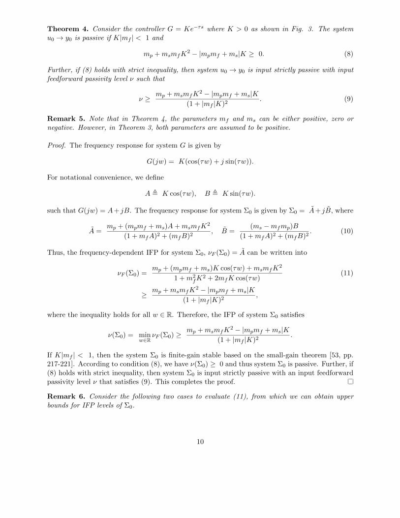
Theorem 4. Consider the controller G = Ke−τs where K > 0 as shown in Fig. 3. The systemu0 → y0 is passive if K|mf | < 1 and
mp +msmfK2 − |mpmf +ms|K ≥ 0. (8)
Further, if (8) holds with strict inequality, then system u0 → y0 is input strictly passive with inputfeedforward passivity level ν such that
ν ≥mp +msmfK
2 − |mpmf +ms|K(1 + |mf |K)2
. (9)
Remark 5. Note that in Theorem 4, the parameters mf and ms can be either positive, zero ornegative. However, in Theorem 3, both parameters are assumed to be positive.
Proof. The frequency response for system G is given by
G(jw) = K(cos(τw) + j sin(τw)).
For notational convenience, we define
A , K cos(τw), B , K sin(τw).
such that G(jw) = A+ jB. The frequency response for system Σ0 is given by Σ0 = A+ jB, where
A =mp + (mpmf +ms)A+msmfK
2
(1 +mfA)2 + (mfB)2, B =
(ms −mfmp)B
(1 +mfA)2 + (mfB)2. (10)
Thus, the frequency-dependent IFP for system Σ0, νF (Σ0) = A can be written into
νF (Σ0) =mp + (mpmf +ms)K cos(τw) +msmfK
2
1 +m2fK
2 + 2mfK cos(τw)(11)
≥mp +msmfK
2 − |mpmf +ms|K(1 + |mf |K)2
,
where the inequality holds for all w ∈ R. Therefore, the IFP of system Σ0 satisfies
ν(Σ0) = minw∈R
νF (Σ0) ≥mp +msmfK
2 − |mpmf +ms|K(1 + |mf |K)2
.
If K|mf | < 1, then the system Σ0 is finite-gain stable based on the small-gain theorem [53, pp.217-221]. According to condition (8), we have ν(Σ0) ≥ 0 and thus system Σ0 is passive. Further, if(8) holds with strict inequality, then system Σ0 is input strictly passive with an input feedforwardpassivity level ν that satisfies (9). This completes the proof.
Remark 6. Consider the following two cases to evaluate (11), from which we can obtain upperbounds for IFP levels of Σ0.
10
(1) If cos(τw) = − 1, e.g. at frequency w = πτ , then we have
νF (Σ0,π
w) =
mp −msK
1−mfK.
Thus, the IFP for system Σ0 satisfies ν ≤ mp−msK1−mfK
.
(2) If cos(τw) = 1, e.g. at frequency w = π2τ , then we have
νF (Σ0,π
2w) =
mp +msK
1 +mfK.
Thus, the IFP for system Σ0 satisfies ν ≤ mp+msK1+mfK
.
The following result can be seen as a generalization of Theorem 2 for feedback interconnections.In Theorem 2, the plant and the controller have to satisfy certain constraints, e.g. one of them hasto be more than passive if the other one is less than passive. If such constraints cannot be satisfied,then we can design the passivation parameters so that the passivity of the feedback system can stillbe guaranteed. The following result is immediate from Theorems 2 and 3.
Theorem 5. Consider the feedback configuration in Fig. 6, where r1 can be seen as the referenceto the controller G. Assume that plant H has OFP level ρ < 0. If the passivation parameters arechosen such that
ν0 =1
2(mp +
ms
mf) > −ρ,
and (7) is satisfied, then the system Σ : r1 → y0 is output strictly passive. Furthermore, the gainof the system Σ is no larger than the value 1
ρ+ν0. �
3.2 Passivation Using Transfer Functions
For the purpose of passivation only, it is sufficient to use constant passivation parameters as inSection 3.1. However, it is often necessary that the system after passivation has other desiredproperties, for instance, being a low pass filter. In the following, we consider the passivationmethod using transfer functions as shown in Fig. 4. Through simple algebraic calculations, we canobtain the transfer function for system u0 → y0 in Fig. 4, which is given by
Π0 =
(mp +msG
1 +mfG
)(as+ 1
bs+ 1
), (12)
where the left bracket represents the system (4) and the right bracket represents the low pass filterH. It is obvious that by adding the low pass filter H in the parallel and series blocks, it is the sameas cascading system (4) (i.e. u0 → y0 in Fig. 3) with H. It is possible to use transfer functions inthe feedback block, however, for simplicity, we assume that mf is a constant in the present report.
11
Gyu
0y0u
Hmp
Hms
fm
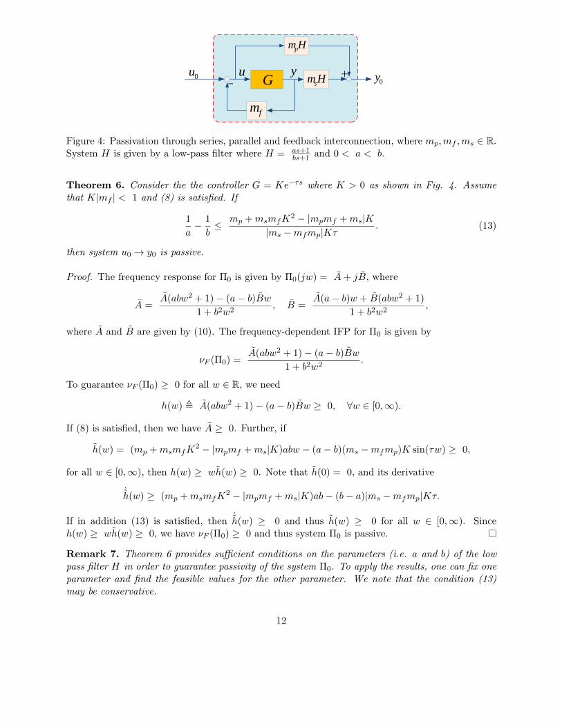
Figure 4: Passivation through series, parallel and feedback interconnection, where mp,mf ,ms ∈ R.System H is given by a low-pass filter where H = as+1
bs+1 and 0 < a < b.
Theorem 6. Consider the the controller G = Ke−τs where K > 0 as shown in Fig. 4. Assumethat K|mf | < 1 and (8) is satisfied. If
1
a− 1
b≤
mp +msmfK2 − |mpmf +ms|K
|ms −mfmp|Kτ. (13)
then system u0 → y0 is passive.
Proof. The frequency response for Π0 is given by Π0(jw) = A+ jB, where
A =A(abw2 + 1)− (a− b)Bw
1 + b2w2, B =
A(a− b)w + B(abw2 + 1)
1 + b2w2,
where A and B are given by (10). The frequency-dependent IFP for Π0 is given by
νF (Π0) =A(abw2 + 1)− (a− b)Bw
1 + b2w2.
To guarantee νF (Π0) ≥ 0 for all w ∈ R, we need
h(w) , A(abw2 + 1)− (a− b)Bw ≥ 0, ∀w ∈ [0,∞).
If (8) is satisfied, then we have A ≥ 0. Further, if
h(w) = (mp +msmfK2 − |mpmf +ms|K)abw − (a− b)(ms −mfmp)K sin(τw) ≥ 0,
for all w ∈ [0,∞), then h(w) ≥ wh(w) ≥ 0. Note that h(0) = 0, and its derivative
˙h(w) ≥ (mp +msmfK
2 − |mpmf +ms|K)ab− (b− a)|ms −mfmp|Kτ.
If in addition (13) is satisfied, then˙h(w) ≥ 0 and thus h(w) ≥ 0 for all w ∈ [0,∞). Since
h(w) ≥ wh(w) ≥ 0, we have νF (Π0) ≥ 0 and thus system Π0 is passive.
Remark 7. Theorem 6 provides sufficient conditions on the parameters (i.e. a and b) of the lowpass filter H in order to guarantee passivity of the system Π0. To apply the results, one can fix oneparameter and find the feasible values for the other parameter. We note that the condition (13)may be conservative.
12

3.3 PI controller with time delay
In Section 3.1 and Section 3.2, we assumed that the controller G is finite-gain stable, which doesnot include the case when the controller G is marginally stable, such as being a PI controller. Inthe following, we present the results for analyzing the IFP level for PI controllers with time delay.
Proposition 1. Consider the pure time-delay transfer function D(s) = e−τs. Then, D(s) hasdelay-independent IFP ν = −1.
Proof. The frequency response for D(s) is given by
D(jw) = e−τjw = cos(τw)− j sin(τw).
Thus, the frequency-dependent IFP is given by
νF (D) = cos(τw) ≥ − 1,
for all w ∈ R. Therefore, the IFP of D(s),
ν(D) = minw∈R
νF (D) ≥ − 1. (14)
On the other hand, when w = πτ , then
νF (D,π
τ) = − 1.
Therefore, we have
ν(D) ≤ νF (D,π
τ) = − 1. (15)
From (14) and (15), we obtain that ν(D) = −1. This completes the proof.
Proposition 2. Consider the transfer function L(s) = 1se−τs. Then, L(s) has IFP ν = −τ .
Proof. The frequency response for L(s) is given by
L(jw) =1
jw(cos(τw)− j sin(τw)).
Thus, the frequency dependent IFP is given by
νF (L) = − 1
wsin(τw).
When w → 0, we have
limw→0
1
wsin(τw) = τ lim
τw→0
1
τwsin(τw)
= τ limτw→0
cos(τw) = τ.
13
Thus, we have νF (L, 0) = − τ and the IFP of L(s) satisfies
ν(L) ≤ νF (L, 0) = − τ. (16)
On the other hand, we have f(w) , νF (L) + τ such that f(0) = 0 and
f(w) =1
w(τw − sin(τw)).
Let us define g(w) , τw − sin(τw) so that g(w) = 0 and
g = τ(1− cos(τw)) ≥ 0.
Thus, g(w) ≥ 0 for all w ≥ 0. Therefore, f(w) ≥ 0 for all w ≥ 0, i.e. νF (L) ≥ − τ . Thus,
ν(L) ≥ − τ. (17)
Based on (16) and (17), we obtain that ν(L) = −τ . This completes the proof.
Remark 8. Consider the case when a transfer function can be written into sums of simple linearmodels, e.g. G = G1 + G2, where G1 and G2 are given by simple linear models. Due to the factthat
ν(G) ≤ ν(G1) + ν(G2), (18)
the IFP for system G can be approximated by the IFP of simpler models G1 and G2.
We consider when G is given by a PI controller cascaded with time-delay, i.e.
G(s) = (Kp +Ki
s)e−τs. (19)
By applying the ‘scaling property’ of the IFP, we can simply calculate the IFP for e−τs and 1se−τs,
which, respectively, are given by −1 and −τ according to Proposition 1-2. Thus, system G(s) givenby (19) has IFP that satisfies
ν(G) ≤ −Kp −Kiτ,
such that Kp +Kiτ is a feedforward gain that can be used to passivate system G(s). The followingresult is immediate.
Theorem 7. Let the controller G be given by (19) and consider the passivation method in Fig. 3.The system Σ0 given by (4) is passive if mp ≥ Kp +Kiτ , mf = 0 and ms = 1.
4 Optimization of Passivation Parameters
The passivation parameters mp,mf ,ms can be selected to optimize system performance in additionto guaranteeing passivity. If the mathematical relation between the performance and the parametersis known, then the performance evaluation can be done directly. If the relation is difficult to obtainor analyze, then the performance can be evaluated through simulation.
14
Initial Parameter Set
Performance Evaluation via Simulation
Current Set of Parameters )(nX
Is PerformanceCriteria Met?
Store Optimal Parameter Set
Yes
Generate New Set of Parameters )1( nX
No
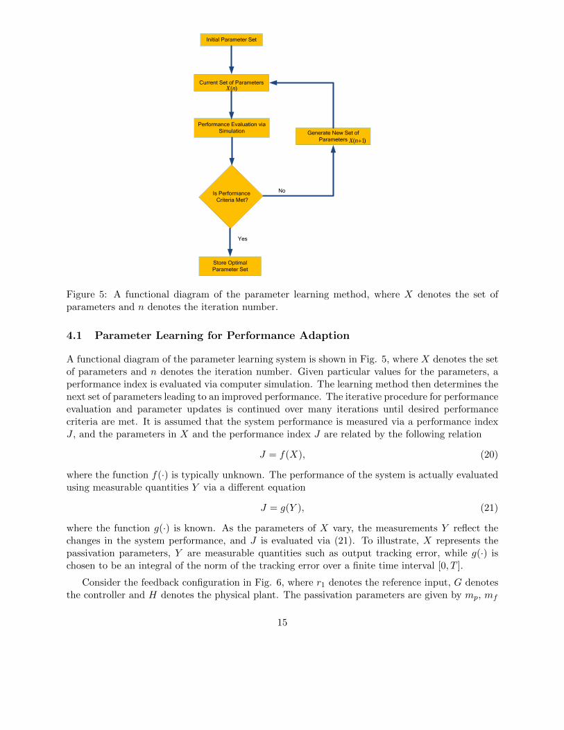
Figure 5: A functional diagram of the parameter learning method, where X denotes the set ofparameters and n denotes the iteration number.
4.1 Parameter Learning for Performance Adaption
A functional diagram of the parameter learning system is shown in Fig. 5, where X denotes the setof parameters and n denotes the iteration number. Given particular values for the parameters, aperformance index is evaluated via computer simulation. The learning method then determines thenext set of parameters leading to an improved performance. The iterative procedure for performanceevaluation and parameter updates is continued over many iterations until desired performancecriteria are met. It is assumed that the system performance is measured via a performance indexJ , and the parameters in X and the performance index J are related by the following relation
J = f(X), (20)
where the function f(·) is typically unknown. The performance of the system is actually evaluatedusing measurable quantities Y via a different equation
J = g(Y ), (21)
where the function g(·) is known. As the parameters of X vary, the measurements Y reflect thechanges in the system performance, and J is evaluated via (21). To illustrate, X represents thepassivation parameters, Y are measurable quantities such as output tracking error, while g(·) ischosen to be an integral of the norm of the tracking error over a finite time interval [0, T ].
Consider the feedback configuration in Fig. 6, where r1 denotes the reference input, G denotesthe controller and H denotes the physical plant. The passivation parameters are given by mp, mf
15
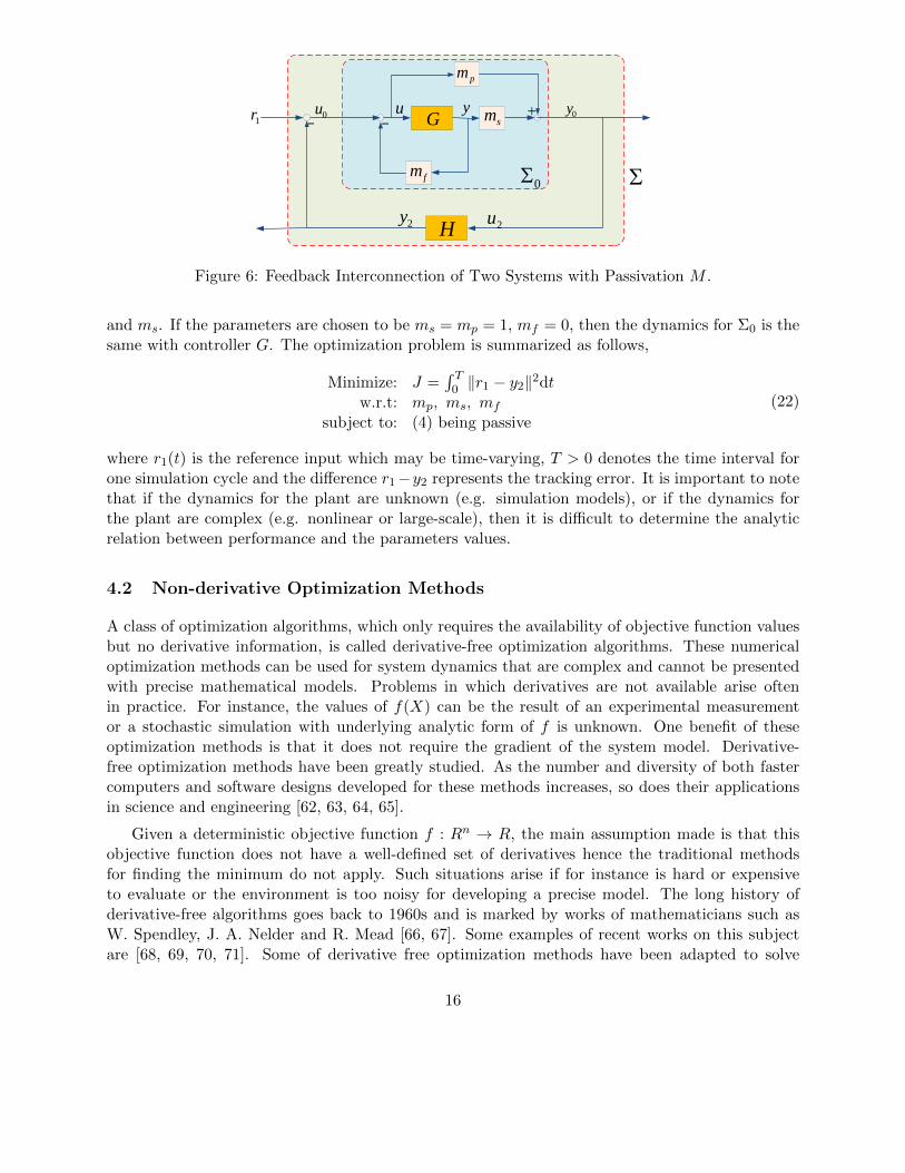
Gyu
0y0u
pm
sm
fm
2y
1r
H
0
2u
Figure 6: Feedback Interconnection of Two Systems with Passivation M .
and ms. If the parameters are chosen to be ms = mp = 1, mf = 0, then the dynamics for Σ0 is thesame with controller G. The optimization problem is summarized as follows,
Minimize: J =∫ T0 ‖r1 − y2‖
2dtw.r.t: mp, ms, mf
subject to: (4) being passive
(22)
where r1(t) is the reference input which may be time-varying, T > 0 denotes the time interval forone simulation cycle and the difference r1−y2 represents the tracking error. It is important to notethat if the dynamics for the plant are unknown (e.g. simulation models), or if the dynamics forthe plant are complex (e.g. nonlinear or large-scale), then it is difficult to determine the analyticrelation between performance and the parameters values.
4.2 Non-derivative Optimization Methods
A class of optimization algorithms, which only requires the availability of objective function valuesbut no derivative information, is called derivative-free optimization algorithms. These numericaloptimization methods can be used for system dynamics that are complex and cannot be presentedwith precise mathematical models. Problems in which derivatives are not available arise oftenin practice. For instance, the values of f(X) can be the result of an experimental measurementor a stochastic simulation with underlying analytic form of f is unknown. One benefit of theseoptimization methods is that it does not require the gradient of the system model. Derivative-free optimization methods have been greatly studied. As the number and diversity of both fastercomputers and software designs developed for these methods increases, so does their applicationsin science and engineering [62, 63, 64, 65].
Given a deterministic objective function f : Rn → R, the main assumption made is that thisobjective function does not have a well-defined set of derivatives hence the traditional methodsfor finding the minimum do not apply. Such situations arise if for instance is hard or expensiveto evaluate or the environment is too noisy for developing a precise model. The long history ofderivative-free algorithms goes back to 1960s and is marked by works of mathematicians such asW. Spendley, J. A. Nelder and R. Mead [66, 67]. Some examples of recent works on this subjectare [68, 69, 70, 71]. Some of derivative free optimization methods have been adapted to solve
16
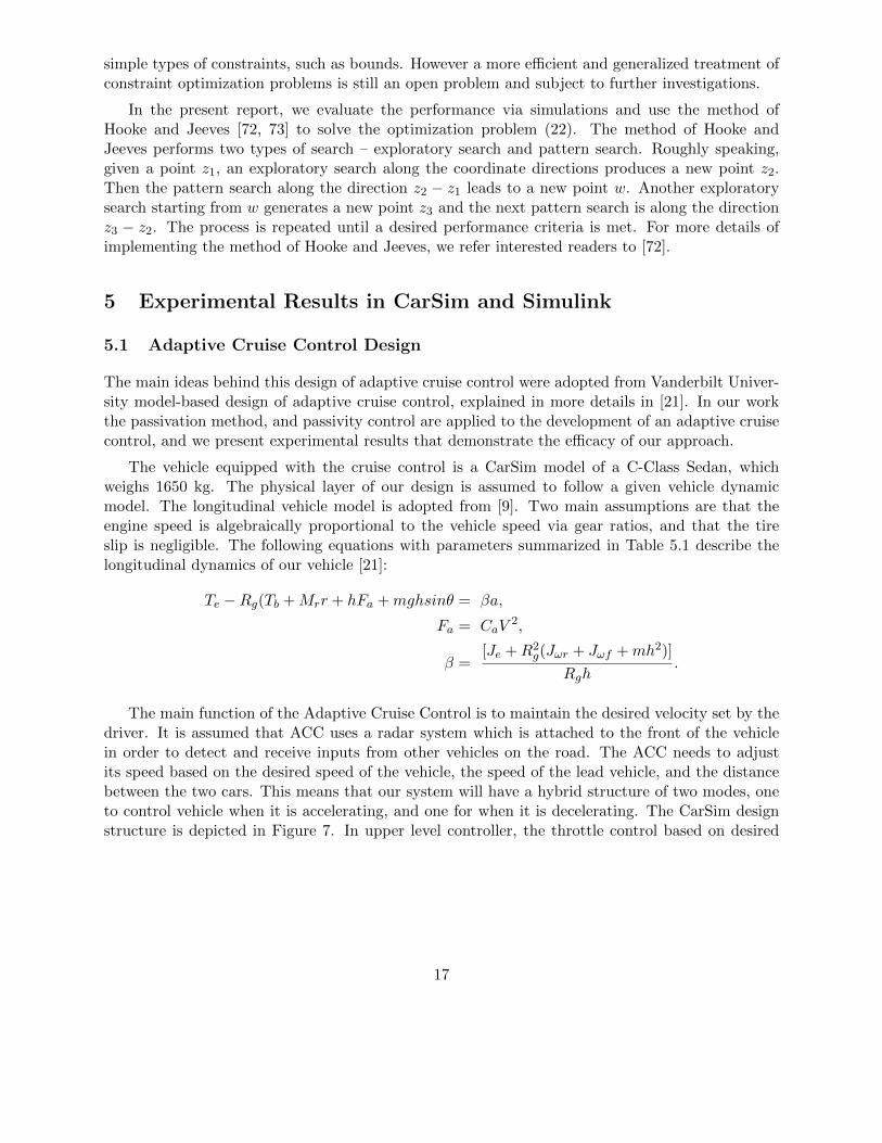
simple types of constraints, such as bounds. However a more efficient and generalized treatment ofconstraint optimization problems is still an open problem and subject to further investigations.
In the present report, we evaluate the performance via simulations and use the method ofHooke and Jeeves [72, 73] to solve the optimization problem (22). The method of Hooke andJeeves performs two types of search – exploratory search and pattern search. Roughly speaking,given a point z1, an exploratory search along the coordinate directions produces a new point z2.Then the pattern search along the direction z2 − z1 leads to a new point w. Another exploratorysearch starting from w generates a new point z3 and the next pattern search is along the directionz3 − z2. The process is repeated until a desired performance criteria is met. For more details ofimplementing the method of Hooke and Jeeves, we refer interested readers to [72].
5 Experimental Results in CarSim and Simulink
5.1 Adaptive Cruise Control Design
The main ideas behind this design of adaptive cruise control were adopted from Vanderbilt Univer-sity model-based design of adaptive cruise control, explained in more details in [21]. In our workthe passivation method, and passivity control are applied to the development of an adaptive cruisecontrol, and we present experimental results that demonstrate the efficacy of our approach.
The vehicle equipped with the cruise control is a CarSim model of a C-Class Sedan, whichweighs 1650 kg. The physical layer of our design is assumed to follow a given vehicle dynamicmodel. The longitudinal vehicle model is adopted from [9]. Two main assumptions are that theengine speed is algebraically proportional to the vehicle speed via gear ratios, and that the tireslip is negligible. The following equations with parameters summarized in Table 5.1 describe thelongitudinal dynamics of our vehicle [21]:
Te −Rg(Tb +Mrr + hFa +mghsinθ = βa,
Fa = CaV2,
β =[Je +R2
g(Jωr + Jωf +mh2)]
Rgh.
The main function of the Adaptive Cruise Control is to maintain the desired velocity set by thedriver. It is assumed that ACC uses a radar system which is attached to the front of the vehiclein order to detect and receive inputs from other vehicles on the road. The ACC needs to adjustits speed based on the desired speed of the vehicle, the speed of the lead vehicle, and the distancebetween the two cars. This means that our system will have a hybrid structure of two modes, oneto control vehicle when it is accelerating, and one for when it is decelerating. The CarSim designstructure is depicted in Figure 7. In upper level controller, the throttle control based on desired
17
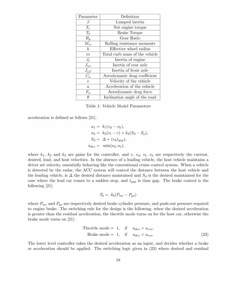
Parameter Definition
β Lumped inertia
Te Net engine torque
Tb Brake Torque
Rg Gear Ratio
Mrr Rolling resistance moments
h Effective wheel radius
m Total curb mass of the vehicle
Je Inertia of engine
Jωr Inertia of rear axle
Jωf Inertia of front axle
Ca Aerodynamic drag coefficient
v Velocity of the vehicle
a Acceleration of the vehicle
Fa Aerodynamic drag force
θ Inclination angle of the road
Table 1: Vehicle Model Parameters
acceleration is defined as follows [21]:
a1 = k1(vd − vh),
a2 = k2(vl − v) + k3(Sd − Sa),Sd = ∆ + (vhtgap),
ades = min(a2, a1).
where k1, k2 and k3 are gains for the controller, and v, vd, vl, vh are respectively the current,desired, lead, and host velocities. In the absence of a leading vehicle, the host vehicle maintains adriver set velocity, essentially behaving like the conventional cruise control system. When a vehicleis detected by the radar, the ACC system will control the distance between the host vehicle andthe leading vehicle, is ∆ the desired distance maintained and Sd is the desired maintained for thecase where the lead car comes to a sudden stop, and tgap is time gap. The brake control is thefollowing [21]:
Tb = kb(Pmc − Ppo)
where Pmc and Ppo are respectively desired brake cylinder pressure, and push-out pressure requiredto engine brake. The switching rule for the design is the following, when the desired accelerationis greater than the residual acceleration, the throttle mode turns on for the host car, otherwise thebrake mode turns on [21]:
Throttle mode = 1, if ades > ares,
Brake mode = 1, if ades < ares. (23)
The lower level controller takes the desired acceleration as an input, and decides whether a brakeor acceleration should be applied. The switching logic given in (23) where desired and residual
18
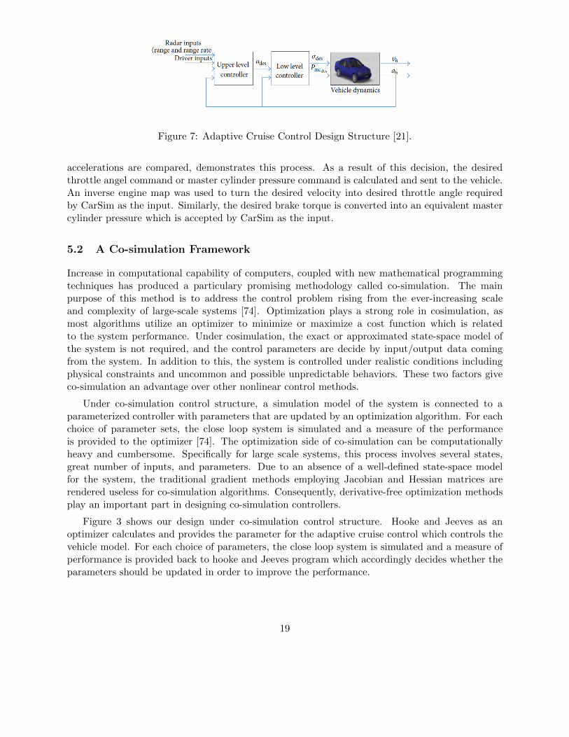
Figure 7: Adaptive Cruise Control Design Structure [21].
accelerations are compared, demonstrates this process. As a result of this decision, the desiredthrottle angel command or master cylinder pressure command is calculated and sent to the vehicle.An inverse engine map was used to turn the desired velocity into desired throttle angle requiredby CarSim as the input. Similarly, the desired brake torque is converted into an equivalent mastercylinder pressure which is accepted by CarSim as the input.
5.2 A Co-simulation Framework
Increase in computational capability of computers, coupled with new mathematical programmingtechniques has produced a particulary promising methodology called co-simulation. The mainpurpose of this method is to address the control problem rising from the ever-increasing scaleand complexity of large-scale systems [74]. Optimization plays a strong role in cosimulation, asmost algorithms utilize an optimizer to minimize or maximize a cost function which is relatedto the system performance. Under cosimulation, the exact or approximated state-space model ofthe system is not required, and the control parameters are decide by input/output data comingfrom the system. In addition to this, the system is controlled under realistic conditions includingphysical constraints and uncommon and possible unpredictable behaviors. These two factors giveco-simulation an advantage over other nonlinear control methods.
Under co-simulation control structure, a simulation model of the system is connected to aparameterized controller with parameters that are updated by an optimization algorithm. For eachchoice of parameter sets, the close loop system is simulated and a measure of the performanceis provided to the optimizer [74]. The optimization side of co-simulation can be computationallyheavy and cumbersome. Specifically for large scale systems, this process involves several states,great number of inputs, and parameters. Due to an absence of a well-defined state-space modelfor the system, the traditional gradient methods employing Jacobian and Hessian matrices arerendered useless for co-simulation algorithms. Consequently, derivative-free optimization methodsplay an important part in designing co-simulation controllers.
Figure 3 shows our design under co-simulation control structure. Hooke and Jeeves as anoptimizer calculates and provides the parameter for the adaptive cruise control which controls thevehicle model. For each choice of parameters, the close loop system is simulated and a measure ofperformance is provided back to hooke and Jeeves program which accordingly decides whether theparameters should be updated in order to improve the performance.
19
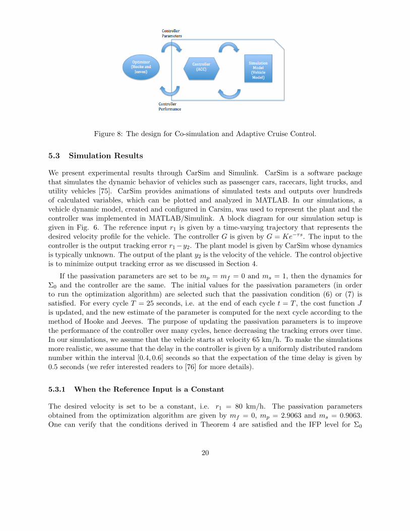
Figure 8: The design for Co-simulation and Adaptive Cruise Control.
5.3 Simulation Results
We present experimental results through CarSim and Simulink. CarSim is a software packagethat simulates the dynamic behavior of vehicles such as passenger cars, racecars, light trucks, andutility vehicles [75]. CarSim provides animations of simulated tests and outputs over hundredsof calculated variables, which can be plotted and analyzed in MATLAB. In our simulations, avehicle dynamic model, created and configured in Carsim, was used to represent the plant and thecontroller was implemented in MATLAB/Simulink. A block diagram for our simulation setup isgiven in Fig. 6. The reference input r1 is given by a time-varying trajectory that represents thedesired velocity profile for the vehicle. The controller G is given by G = Ke−τs. The input to thecontroller is the output tracking error r1−y2. The plant model is given by CarSim whose dynamicsis typically unknown. The output of the plant y2 is the velocity of the vehicle. The control objectiveis to minimize output tracking error as we discussed in Section 4.
If the passivation parameters are set to be mp = mf = 0 and ms = 1, then the dynamics forΣ0 and the controller are the same. The initial values for the passivation parameters (in orderto run the optimization algorithm) are selected such that the passivation condition (6) or (7) issatisfied. For every cycle T = 25 seconds, i.e. at the end of each cycle t = T , the cost function Jis updated, and the new estimate of the parameter is computed for the next cycle according to themethod of Hooke and Jeeves. The purpose of updating the passivation parameters is to improvethe performance of the controller over many cycles, hence decreasing the tracking errors over time.In our simulations, we assume that the vehicle starts at velocity 65 km/h. To make the simulationsmore realistic, we assume that the delay in the controller is given by a uniformly distributed randomnumber within the interval [0.4, 0.6] seconds so that the expectation of the time delay is given by0.5 seconds (we refer interested readers to [76] for more details).
5.3.1 When the Reference Input is a Constant
The desired velocity is set to be a constant, i.e. r1 = 80 km/h. The passivation parametersobtained from the optimization algorithm are given by mf = 0, mp = 2.9063 and ms = 0.9063.One can verify that the conditions derived in Theorem 4 are satisfied and the IFP level for Σ0
20
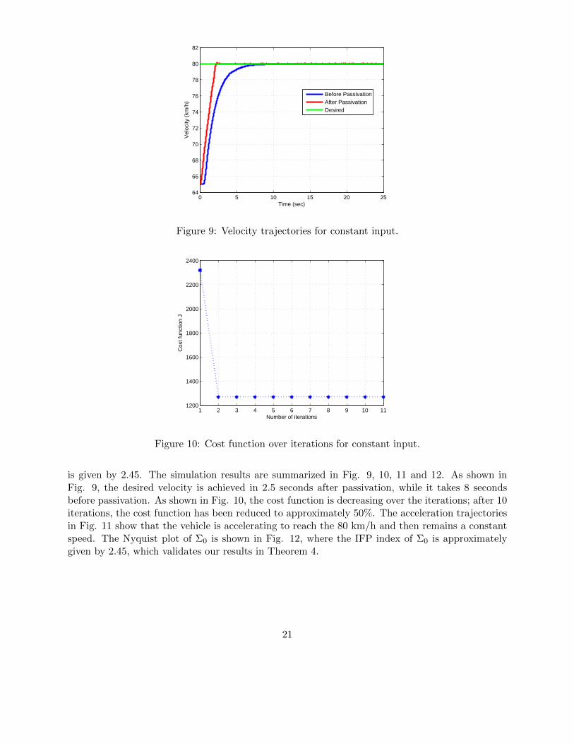
0 5 10 15 20 2564
66
68
70
72
74
76
78
80
82
Time (sec)
Vel
ocity
(km
/h)
Before PassivationAfter PassivationDesired
Figure 9: Velocity trajectories for constant input.
1 2 3 4 5 6 7 8 9 10 111200
1400
1600
1800
2000
2200
2400
Cos
t fun
ctio
n J
Number of iterations
Figure 10: Cost function over iterations for constant input.
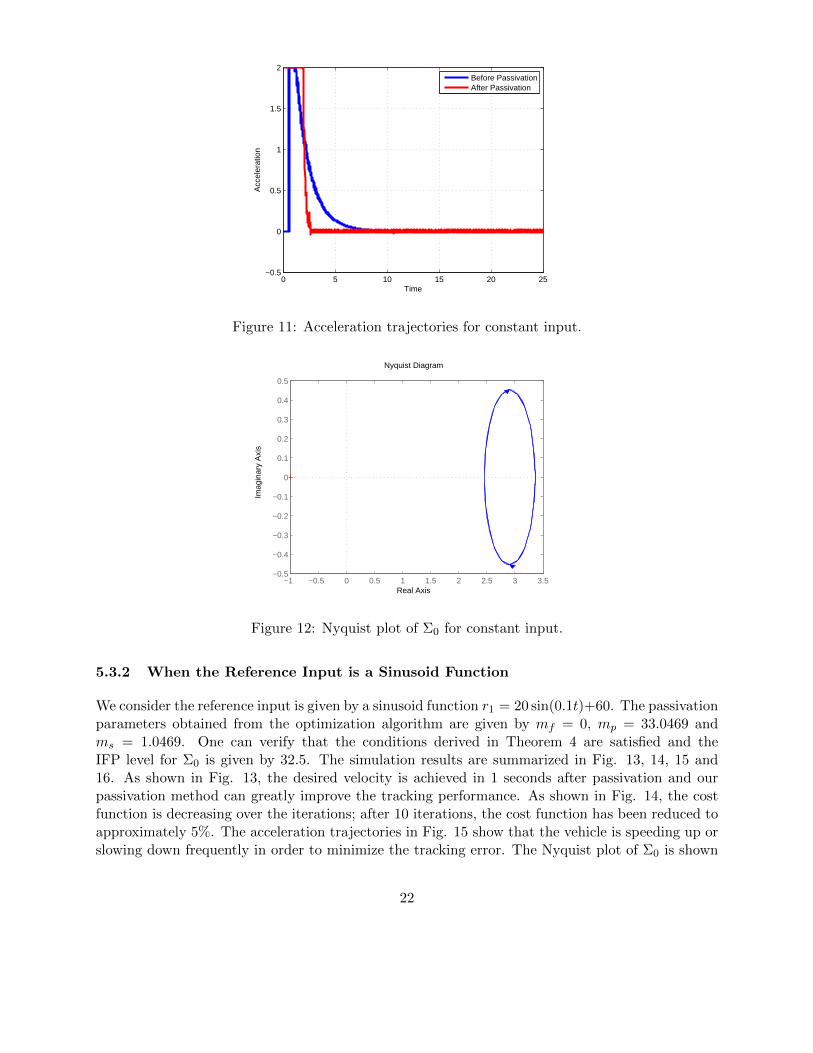
is given by 2.45. The simulation results are summarized in Fig. 9, 10, 11 and 12. As shown inFig. 9, the desired velocity is achieved in 2.5 seconds after passivation, while it takes 8 secondsbefore passivation. As shown in Fig. 10, the cost function is decreasing over the iterations; after 10iterations, the cost function has been reduced to approximately 50%. The acceleration trajectoriesin Fig. 11 show that the vehicle is accelerating to reach the 80 km/h and then remains a constantspeed. The Nyquist plot of Σ0 is shown in Fig. 12, where the IFP index of Σ0 is approximatelygiven by 2.45, which validates our results in Theorem 4.
21
0 5 10 15 20 25−0.5
0
0.5
1
1.5
2
Time
Acc
eler
atio
n
Before PassivationAfter Passivation
Figure 11: Acceleration trajectories for constant input.
−1 −0.5 0 0.5 1 1.5 2 2.5 3 3.5−0.5
−0.4
−0.3
−0.2
−0.1
0
0.1
0.2
0.3
0.4
0.5
Nyquist Diagram
Real Axis
Imag
inar
y A
xis
Figure 12: Nyquist plot of Σ0 for constant input.
5.3.2 When the Reference Input is a Sinusoid Function
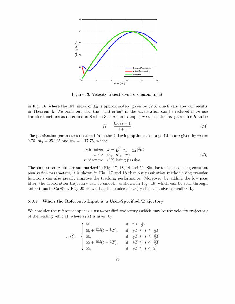
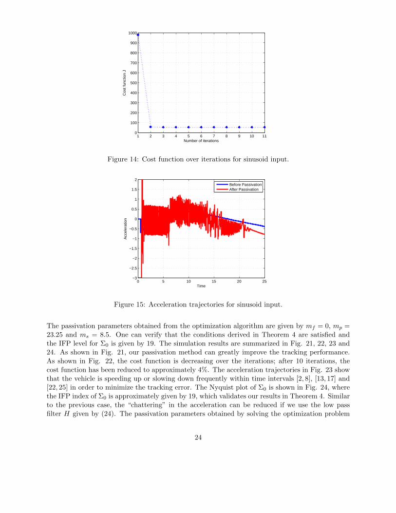
We consider the reference input is given by a sinusoid function r1 = 20 sin(0.1t)+60. The passivationparameters obtained from the optimization algorithm are given by mf = 0, mp = 33.0469 andms = 1.0469. One can verify that the conditions derived in Theorem 4 are satisfied and theIFP level for Σ0 is given by 32.5. The simulation results are summarized in Fig. 13, 14, 15 and16. As shown in Fig. 13, the desired velocity is achieved in 1 seconds after passivation and ourpassivation method can greatly improve the tracking performance. As shown in Fig. 14, the costfunction is decreasing over the iterations; after 10 iterations, the cost function has been reduced toapproximately 5%. The acceleration trajectories in Fig. 15 show that the vehicle is speeding up orslowing down frequently in order to minimize the tracking error. The Nyquist plot of Σ0 is shown
22
0 5 10 15 20 2560
65
70
75
80
85
Time (sec)
Vel
ocity
(km
/h)
Before PassivationAfter PassivationDesired
Figure 13: Velocity trajectories for sinusoid input.
in Fig. 16, where the IFP index of Σ0 is approximately given by 32.5, which validates our resultsin Theorem 4. We point out that the “chattering” in the acceleration can be reduced if we usetransfer functions as described in Section 3.2. As an example, we select the low pass filter H to be
H =0.08s+ 1
s+ 1. (24)
The passivation parameters obtained from the following optimization algorithm are given by mf =0.75, mp = 25.125 and ms = −17.75, where
Minimize: J =∫ T0 ‖r1 − y2‖
2dtw.r.t: mp, ms, mf
subject to: (12) being passive
(25)
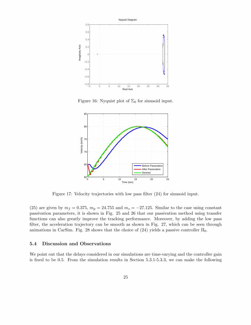
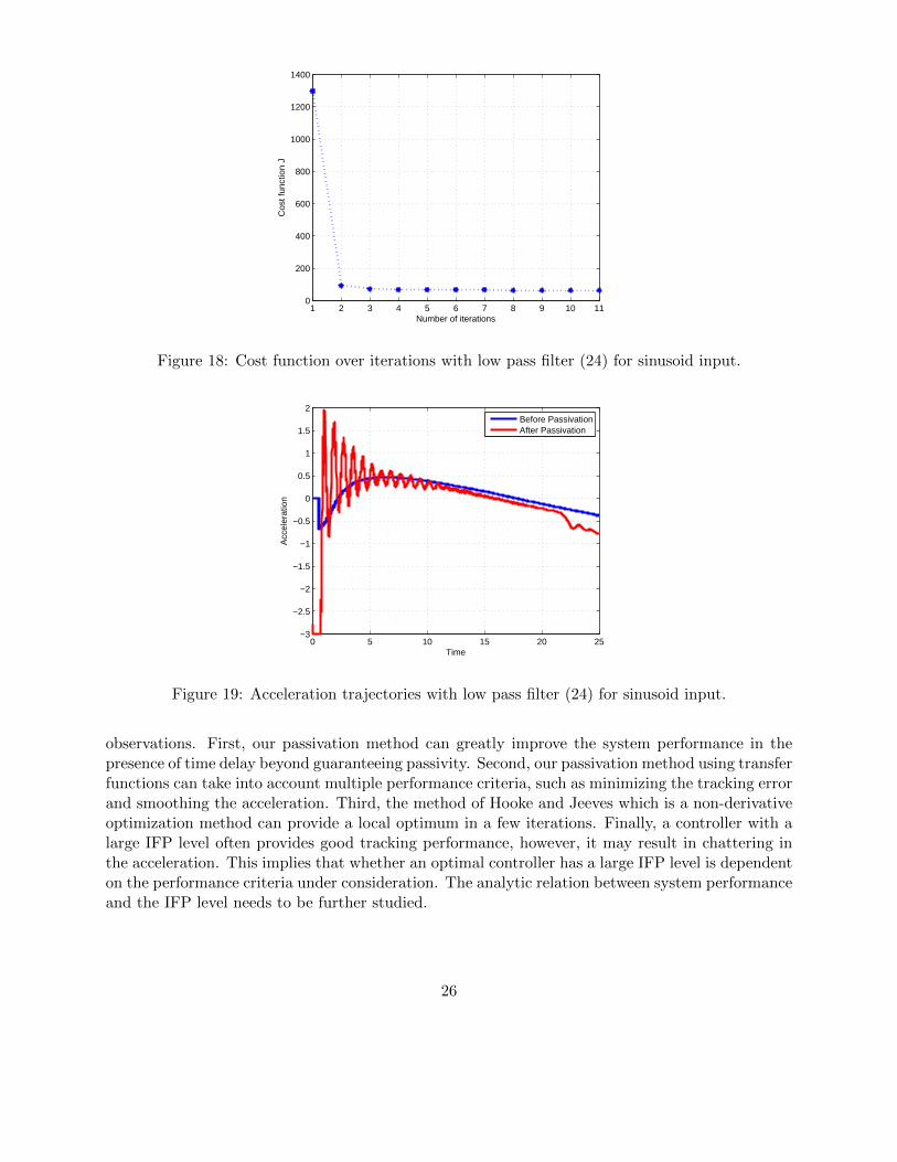
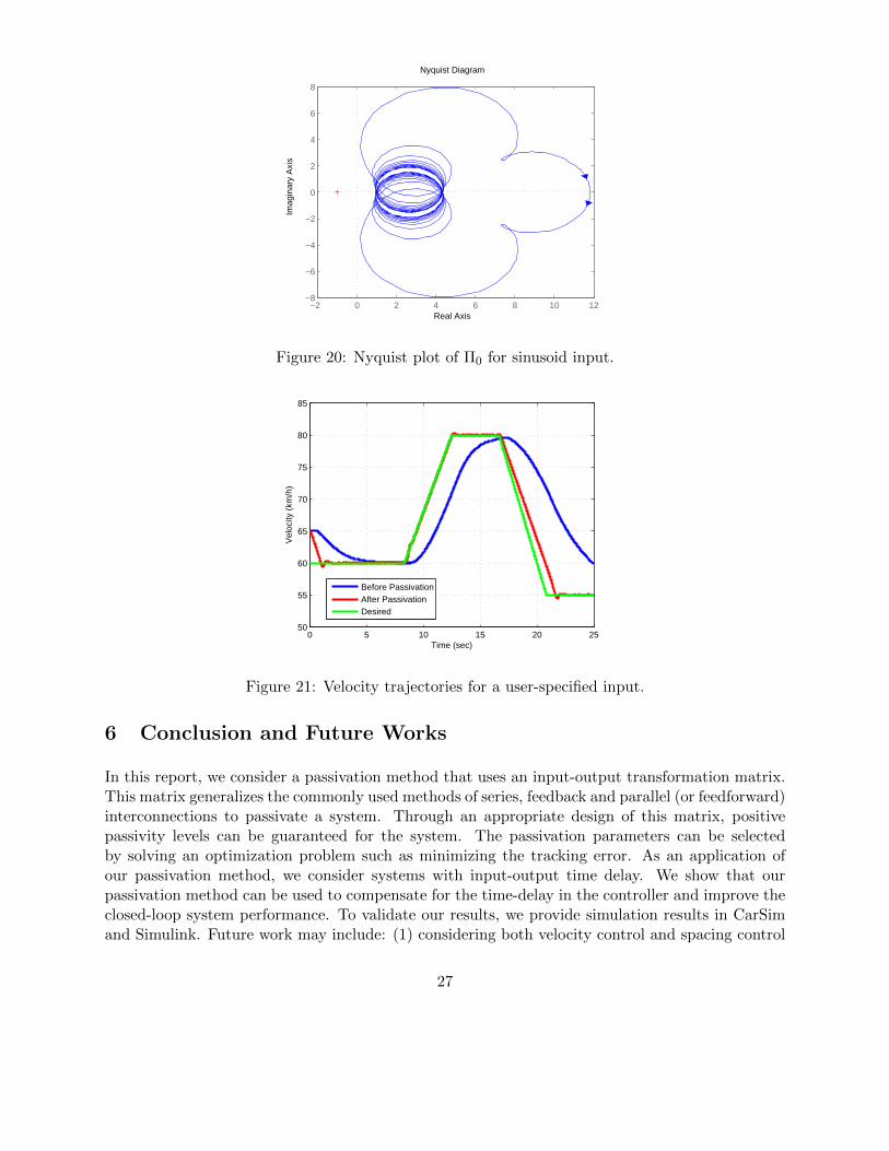
The simulation results are summarized in Fig. 17, 18, 19 and 20. Similar to the case using constantpassivation parameters, it is shown in Fig. 17 and 18 that our passivation method using transferfunctions can also greatly improve the tracking performance. Moreover, by adding the low passfilter, the acceleration trajectory can be smooth as shown in Fig. 19, which can be seen throughanimations in CarSim. Fig. 20 shows that the choice of (24) yields a passive controller Π0.
5.3.3 When the Reference Input is a User-Specified Trajectory
We consider the reference input is a user-specified trajectory (which may be the velocity trajectoryof the leading vehicle), where r1(t) is given by
r1(t) =
60, if t ≤ 13T
60 + 120T (t− 1
3T ), if 13T ≤ t ≤ 1
2T
80, if 12T ≤ t ≤ 2
3T
55 + 150T (t− 5
6T ), if 23T ≤ t ≤ 5
6T
55, if 56T ≤ t ≤ T
23
1 2 3 4 5 6 7 8 9 10 110
100
200
300
400
500
600
700
800
900
1000
Cos
t fun
ctio
n J
Number of iterations
Figure 14: Cost function over iterations for sinusoid input.
0 5 10 15 20 25−3
−2.5
−2
−1.5
−1
−0.5
0
0.5
1
1.5
2
Time
Acc
eler
atio
n
Before PassivationAfter Passivation
Figure 15: Acceleration trajectories for sinusoid input.
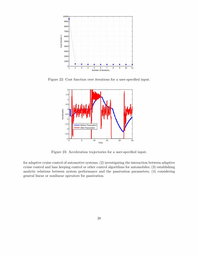
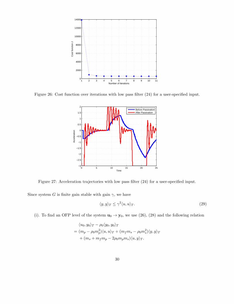
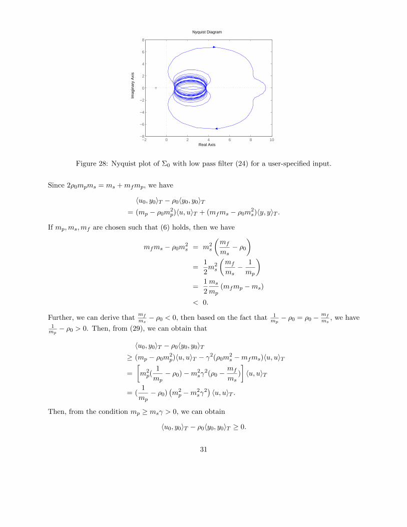
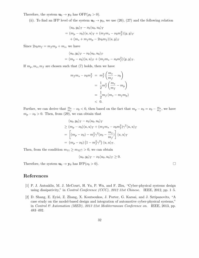
The passivation parameters obtained from the optimization algorithm are given by mf = 0, mp =23.25 and ms = 8.5. One can verify that the conditions derived in Theorem 4 are satisfied andthe IFP level for Σ0 is given by 19. The simulation results are summarized in Fig. 21, 22, 23 and24. As shown in Fig. 21, our passivation method can greatly improve the tracking performance.As shown in Fig. 22, the cost function is decreasing over the iterations; after 10 iterations, thecost function has been reduced to approximately 4%. The acceleration trajectories in Fig. 23 showthat the vehicle is speeding up or slowing down frequently within time intervals [2, 8], [13, 17] and[22, 25] in order to minimize the tracking error. The Nyquist plot of Σ0 is shown in Fig. 24, wherethe IFP index of Σ0 is approximately given by 19, which validates our results in Theorem 4. Similarto the previous case, the “chattering” in the acceleration can be reduced if we use the low passfilter H given by (24). The passivation parameters obtained by solving the optimization problem
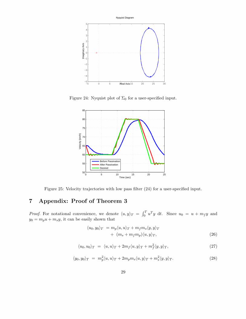
24
Nyquist Diagram
Real Axis
Imag
inar
y A
xis
−5 0 5 10 15 20 25 30 35−0.8
−0.6
−0.4
−0.2
0
0.2
0.4
0.6
0.8
Figure 16: Nyquist plot of Σ0 for sinusoid input.
0 5 10 15 20 2560
65
70
75
80
85
Time (sec)
Vel
ocity
(km
/h)
Before PassivationAfter PassivationDesired
Figure 17: Velocity trajectories with low pass filter (24) for sinusoid input.
(25) are given by mf = 0.375, mp = 24.755 and ms = −27.125. Similar to the case using constantpassivation parameters, it is shown in Fig. 25 and 26 that our passivation method using transferfunctions can also greatly improve the tracking performance. Moreover, by adding the low passfilter, the acceleration trajectory can be smooth as shown in Fig. 27, which can be seen throughanimations in CarSim. Fig. 28 shows that the choice of (24) yields a passive controller Π0.
5.4 Discussion and Observations
We point out that the delays considered in our simulations are time-varying and the controller gainis fixed to be 0.5. From the simulation results in Section 5.3.1-5.3.3, we can make the following
25
1 2 3 4 5 6 7 8 9 10 110
200
400
600
800
1000
1200
1400
Cos
t fun
ctio
n J
Number of iterations
Figure 18: Cost function over iterations with low pass filter (24) for sinusoid input.
0 5 10 15 20 25−3
−2.5
−2
−1.5
−1
−0.5
0
0.5
1
1.5
2
Time
Acc
eler
atio
n
Before PassivationAfter Passivation
Figure 19: Acceleration trajectories with low pass filter (24) for sinusoid input.
observations. First, our passivation method can greatly improve the system performance in thepresence of time delay beyond guaranteeing passivity. Second, our passivation method using transferfunctions can take into account multiple performance criteria, such as minimizing the tracking errorand smoothing the acceleration. Third, the method of Hooke and Jeeves which is a non-derivativeoptimization method can provide a local optimum in a few iterations. Finally, a controller with alarge IFP level often provides good tracking performance, however, it may result in chattering inthe acceleration. This implies that whether an optimal controller has a large IFP level is dependenton the performance criteria under consideration. The analytic relation between system performanceand the IFP level needs to be further studied.
26
−2 0 2 4 6 8 10 12−8
−6
−4
−2
0
2
4
6
8
Nyquist Diagram
Real Axis
Imag
inar
y A
xis
Figure 20: Nyquist plot of Π0 for sinusoid input.
0 5 10 15 20 2550
55
60
65
70
75
80
85
Time (sec)
Vel
ocity
(km
/h)
Before PassivationAfter PassivationDesired
Figure 21: Velocity trajectories for a user-specified input.
6 Conclusion and Future Works
In this report, we consider a passivation method that uses an input-output transformation matrix.This matrix generalizes the commonly used methods of series, feedback and parallel (or feedforward)interconnections to passivate a system. Through an appropriate design of this matrix, positivepassivity levels can be guaranteed for the system. The passivation parameters can be selectedby solving an optimization problem such as minimizing the tracking error. As an application ofour passivation method, we consider systems with input-output time delay. We show that ourpassivation method can be used to compensate for the time-delay in the controller and improve theclosed-loop system performance. To validate our results, we provide simulation results in CarSimand Simulink. Future work may include: (1) considering both velocity control and spacing control
27
1 2 3 4 5 6 7 8 9 10 110
1000
2000
3000
4000
5000
6000
7000
8000
9000
10000
Cos
t fun
ctio
n J
Number of iterations
Figure 22: Cost function over iterations for a user-specified input.
0 5 10 15 20 25−3
−2.5
−2
−1.5
−1
−0.5
0
0.5
1
1.5
2
Time
Acc
eler
atio
n
Before PassivationAfter Passivation
Figure 23: Acceleration trajectories for a user-specified input.
for adaptive cruise control of automotive systems; (2) investigating the interaction between adaptivecruise control and lane keeping control or other control algorithms for automobiles; (3) establishinganalytic relations between system performance and the passivation parameters; (4) consideringgeneral linear or nonlinear operators for passivation.
28
Nyquist Diagram
Real AxisIm
agin
ary
Axi
s−5 0 5 10 15 20 25 30
−5
−4
−3
−2
−1
0
1
2
3
4
5
Figure 24: Nyquist plot of Σ0 for a user-specified input.
0 5 10 15 20 2550
55
60
65
70
75
80
85
Time (sec)
Vel
ocity
(km
/h)
Before PassivationAfter PassivationDesired
Figure 25: Velocity trajectories with low pass filter (24) for a user-specified input.
7 Appendix: Proof of Theorem 3
Proof. For notational convenience, we denote 〈u, y〉T =∫ T0 uT y dt. Since u0 = u + mfy and
y0 = mpu+msy, it can be easily shown that
〈u0, y0〉T = mp〈u, u〉T +mfms〈y, y〉T+ (ms +mfmp)〈u, y〉T , (26)
〈u0, u0〉T = 〈u, u〉T + 2mf 〈u, y〉T +m2f 〈y, y〉T , (27)
〈y0, y0〉T = m2p〈u, u〉T + 2mpms〈u, y〉T +m2
s〈y, y〉T . (28)
29
1 2 3 4 5 6 7 8 9 10 110
2000
4000
6000
8000
10000
12000
14000
Cos
t fun
ctio
n J
Number of iterations
Figure 26: Cost function over iterations with low pass filter (24) for a user-specified input.
0 5 10 15 20 25−3
−2.5
−2
−1.5
−1
−0.5
0
0.5
1
1.5
2
Time
Acc
eler
atio
n
Before PassivationAfter Passivation
Figure 27: Acceleration trajectories with low pass filter (24) for a user-specified input.
Since system G is finite gain stable with gain γ, we have
〈y, y〉T ≤ γ2〈u, u〉T . (29)
(i). To find an OFP level of the system u0 → y0, we use (26), (28) and the following relation
〈u0, y0〉T − ρ0〈y0, y0〉T= (mp − ρ0m2
p)〈u, u〉T + (mfms − ρ0m2s)〈y, y〉T
+ (ms +mfmp − 2ρ0mpms)〈u, y〉T .
30
−2 0 2 4 6 8 10−8
−6
−4
−2
0
2
4
6
8
Nyquist Diagram
Real Axis
Imag
inar
y A
xis
Figure 28: Nyquist plot of Σ0 with low pass filter (24) for a user-specified input.
Since 2ρ0mpms = ms +mfmp, we have
〈u0, y0〉T − ρ0〈y0, y0〉T= (mp − ρ0m2
p)〈u, u〉T + (mfms − ρ0m2s)〈y, y〉T .
If mp,ms,mf are chosen such that (6) holds, then we have
mfms − ρ0m2s = m2
s
(mf
ms− ρ0
)=
1
2m2s
(mf
ms− 1
mp
)=
1
2
ms
mp(mfmp −ms)
< 0.
Further, we can derive thatmf
ms− ρ0 < 0, then based on the fact that 1
mp− ρ0 = ρ0 −
mf
ms, we have
1mp− ρ0 > 0. Then, from (29), we can obtain that
〈u0, y0〉T − ρ0〈y0, y0〉T≥ (mp − ρ0m2
p)〈u, u〉T − γ2(ρ0m2s −mfms)〈u, u〉T
=
[m2p(
1
mp− ρ0)−m2
sγ2(ρ0 −
mf
ms)
]〈u, u〉T
= (1
mp− ρ0)
(m2p −m2
sγ2)〈u, u〉T .
Then, from the condition mp ≥ msγ > 0, we can obtain
〈u0, y0〉T − ρ0〈y0, y0〉T ≥ 0.
31
Therefore, the system u0 → y0 has OFP(ρ0 > 0).
(ii). To find an IFP level of the system u0 → y0, we use (26), (27) and the following relation
〈u0, y0〉T − ν0〈u0, u0〉T= (mp − ν0)〈u, u〉T + (mfms − ν0m2
f )〈y, y〉T+ (ms +mfmp − 2ν0mf )〈u, y〉T
Since 2ν0mf = mfmp +ms, we have
〈u0, y0〉T − ν0〈u0, u0〉T= (mp − ν0)〈u, u〉T + (mfms − ν0m2
f )〈y, y〉T .
If mp,ms,mf are chosen such that (7) holds, then we have
mfms − ν0m2f = m2
f
(ms
mf− ν0
)=
1
2m2f
(ms
mf−mp
)=
1
2mf (ms −mfmp)
< 0.
Further, we can derive that msmf− ν0 < 0, then based on the fact that mp − ν0 = ν0 − ms
mf, we have
mp − ν0 > 0. Then, from (29), we can obtain that
〈u0, y0〉T − ν0〈u0, u0〉T≥ (mp − ν0)〈u, u〉T + (mfms − ν0m2
f )γ2〈u, u〉T
=
[(mp − ν0)−m2
fγ2(ν0 −
ms
mf)
]〈u, u〉T
= (mp − ν0)(1−m2
fγ2)〈u, u〉T .
Then, from the condition m11 ≥ m12γ > 0, we can obtain
〈u0, y0〉T − ν0〈u0, u0〉T ≥ 0.
Therefore, the system u0 → y0 has IFP(ν0 > 0).
References
[1] P. J. Antsaklis, M. J. McCourt, H. Yu, P. Wu, and F. Zhu, “Cyber-physical systems designusing dissipativity,” in Control Conference (CCC), 2012 31st Chinese. IEEE, 2012, pp. 1–5.
[2] D. Shang, E. Eyisi, Z. Zhang, X. Koutsoukos, J. Porter, G. Karsai, and J. Sztipanovits, “Acase study on the model-based design and integration of automotive cyber-physical systems,”in Control & Automation (MED), 2013 21st Mediterranean Conference on. IEEE, 2013, pp.483–492.
32
[3] J. Bao and P. L. Lee, Process control: the passive systems approach. Springer Science &Business Media, 2007.
[4] D. Hill and P. Moylan, “The stability of nonlinear dissipative systems,” Automatic Control,IEEE Transactions on, vol. 21, no. 5, pp. 708 – 711, Oct. 1976.
[5] R. Ortega, A. J. Van Der Schaft, I. Mareels, and B. Maschke, “Putting energy back in control,”Control Systems, IEEE, vol. 21, no. 2, pp. 18–33, 2001.
[6] M. Zefran, F. Bullo, and M. Stein, “A notion of passivity for hybrid systems,” in Decision andControl, 2001. Proceedings of the 40th IEEE Conference on, vol. 1. IEEE, 2001, pp. 768–773.
[7] J. Zhao and D. J. Hill, “Dissipativity theory for switched systems,” Automatic Control, IEEETransactions on, vol. 53, no. 4, pp. 941–953, 2008.
[8] J. Gerdes and J. Hedrick, “Vehicle speed and spacing control via coordinated throttle andbrake actuation,” Control Engineering Practice, vol. 5, no. 11, pp. 1607–1614, 1997.
[9] J. Hedrick and P. Yip, “Multiple sliding surface control: theory and application,” Journal ofdynamic systems, measurement, and control, vol. 122, no. 4, pp. 586–593, 2000.
[10] P. A. Ioannou and C.-C. Chien, “Autonomous intelligent cruise control,” Vehicular Technology,IEEE Transactions on, vol. 42, no. 4, pp. 657–672, 1993.
[11] K. Yi, S. Lee, and Y. Kwon, “An investigation of intelligent cruise control laws for passengervehicles,” Proceedings of the Institution of Mechanical Engineers, Part D: Journal of Automo-bile Engineering, vol. 215, no. 2, pp. 159–169, 2001.
[12] P. Fancher, H. Peng, and Z. Bareket, “Comparative analyses of three types of headway controlsystems for heavy commercial vehicles,” Vehicle System Dynamics, vol. 25, no. S1, pp. 139–151,1996.
[13] B. A. Guvenc and E. Kural, “Adaptive cruise control simulator: a low-cost, multiple-driver-in-the-loop simulator,” Control Systems, IEEE, vol. 26, no. 3, pp. 42–55, 2006.
[14] K. Breuer and M. Weilkes, “A versatile test-vehicle for acc-systems and components,” inEuromotor-Seminar Telematic/Vehicle and Environment-” Adaptive Cruise Control, SeriesIntroduction and Future Development, 1999.
[15] A. R. Girard, S. Spry, and J. K. Hedrick, “Intelligent cruise control applications: Real-timeembedded hybrid control software,” Robotics & Automation Magazine, IEEE, vol. 12, no. 1,pp. 22–28, 2005.
[16] H. Raza and P. Ioannou, “Vehicle following control design for automated highway systems,”Control Systems, IEEE, vol. 16, no. 6, pp. 43–60, 1996.
[17] X.-Y. Lu, H.-S. Tan, S. Shladover, and J. K. Hedrick, “Nonlinear longitudinal controller imple-mentation and comparison for automated cars,” Journal of Dynamic Systems, Measurement,and Control, vol. 123, no. 2, pp. 161–167, 2001.
33
[18] S. Dermann and R. Isermann, “Nonlinear distance and cruise control for passenger cars,” inAmerican Control Conference, Proceedings of the 1995, vol. 5. IEEE, 1995, pp. 3081–3085.
[19] H. Holzmann, C. Halfmann, S. Germann, M. Wurtenberger, and R. Isermann, “Longitudinaland lateral control and supervision of autonomous intelligent vehicles,” Control EngineeringPractice, vol. 5, no. 11, pp. 1599–1605, 1997.
[20] A. Stefanopoulou and L. Moklegaard, “Adaptive continuously variable compression brakingcontrol for heavy-duty vehicles,” Ann Arbor, vol. 1001, p. 48197, 2002.
[21] E. Eyisi, Z. Zhang, X. Koutsoukos, J. Porter, G. Karsai, and J. Sztipanovits, “Model-basedcontrol design and integration of cyberphysical systems: an adaptive cruise control case study,”Journal of Control Science and Engineering, vol. 2013, p. 1, 2013.
[22] Q.-G. Wang, T. H. Lee, and K. K. Tan, Finite-spectrum assignment for time-delay systems.Springer Science & Business Media, 1998, vol. 239.
[23] O. J. Smith, “A controller to overcome dead time,” ISA Journal, vol. 6, no. 2, pp. 28–33, 1959.
[24] J. Jang et al., “Adaptive control design with guaranteed margins for nonlinear plants,” Ph.D.dissertation, Massachusetts Institute of Technology, 2009.
[25] S.-I. Niculescu and A. M. Annaswamy, “An adaptive smith-controller for time-delay systemswith relative degree n 2,” Systems & control letters, vol. 49, no. 5, pp. 347–358, 2003.
[26] D. Kim and J. Park, “Application of adaptive control to the fluctuation of engine speed atidle,” Information Sciences, vol. 177, no. 16, pp. 3341–3355, 2007.
[27] R. Ortega and R. Lozano, “Globally stable adaptive controller for systems with delay,” Inter-national Journal of Control, vol. 47, no. 1, pp. 17–23, 1988.
[28] V. Kolmanovskii and A. Myshkis, Introduction to the theory and applications of functionaldifferential equations. Springer Science & Business Media, 1999, vol. 463.
[29] S.-I. Niculescu, Delay effects on stability: a robust control approach. Springer Science &Business Media, 2001, vol. 269.
[30] J.-P. Richard, “Time-delay systems: an overview of some recent advances and open problems,”automatica, vol. 39, no. 10, pp. 1667–1694, 2003.
[31] K. Gu and S.-I. Niculescu, “Survey on recent results in the stability and control of time-delay systems*,” Journal of Dynamic Systems, Measurement, and Control, vol. 125, no. 2, pp.158–165, 2003.
[32] T. Legouis, A. Laneville, P. Bourassa, and G. Payre, “Characterization of dynamic vehiclestability using two models of the human pilot behaviour,” Vehicle System Dynamics, vol. 15,no. 1, pp. 1–18, 1986.
[33] K. Guo and H. Guan, “Modelling of driver/vehicle directional control system,” Vehicle SystemDynamics, vol. 22, no. 3-4, pp. 141–184, 1993.
34
[34] D. T. McRuer and E. S. Krendel, “Mathematical models of human pilot behavior,” DTICDocument, Tech. Rep., 1974.
[35] Z. Liu, G. Payre, and P. Bourassa, “Nonlinear oscillations and chaotic motions in a road vehiclesystem with driver steering control,” Nonlinear Dynamics, vol. 9, no. 3, pp. 281–304, 1996.
[36] G. Orosz and G. Stepan, “Subcritical hopf bifurcations in a car-following model with reaction-time delay,” Proceedings of the Royal Society A: Mathematical, Physical and Engineering Sci-ence, vol. 462, no. 2073, pp. 2643–2670, 2006.
[37] L. Davis, “Stability of adaptive cruise control systems taking account of vehicle response timeand delay,” Physics Letters A, vol. 376, no. 40, pp. 2658–2662, 2012.
[38] M. Bando, K. Hasebe, K. Nakanishi, and A. Nakayama, “Analysis of optimal velocity modelwith explicit delay,” Physical Review E, vol. 58, no. 5, p. 5429, 1998.
[39] T. Nagatani and K. Nakanishi, “Delay effect on phase transitions in traffic dynamics,” PhysicalReview E, vol. 57, no. 6, p. 6415, 1998.
[40] G. Orosz, J. Moehlis, and F. Bullo, “Robotic reactions: Delay-induced patterns in autonomousvehicle systems,” Physical Review E, vol. 81, no. 2, p. 025204, 2010.
[41] ——, “Delayed car-following dynamics for human and robotic drivers,” in ASME 2011 Inter-national Design Engineering Technical Conferences and Computers and Information in Engi-neering Conference. American Society of Mechanical Engineers, 2011, pp. 529–538.
[42] C. Scherer, P. Gahinet, and M. Chilali, “Multiobjective output-feedback control via lmi opti-mization,” Automatic Control, IEEE Transactions on, vol. 42, no. 7, pp. 896–911, Jul 1997.
[43] M. Xia, P. Antsaklis, and V. Gupta, “Passivity analysis of a system and its approximation,”in American Control Conference (ACC), 2013, June 2013, pp. 296–301.
[44] R. Lozano, B. Brogliato, O.Egeland, and B. Maschke, Dissipative Systems Analysis and Con-trol: Theory and Applications, 1st ed. London: Springer, 2000.
[45] J. R. Forbes and C. J. Damaren, “Design of optimal strictly positive real controllers usingnumerical optimization for the control of flexible robotic systems,” Journal of the FranklinInstitute, vol. 348, no. 8, pp. 2191 – 2215, 2011.
[46] A. van der Schaft, L2-Gain and Passivity Techniques in Nonlinear Control, 2nd ed. Springer,2000.
[47] R. Sepulchre, M. Jankovic, and P. Kokotovic, Constructive Nonlinear Control. Springer, 1994.
[48] H. Yu, F. Zhu, M. Xia, and P. J. Antsaklis, “Robust stabilizing output feedback nonlinearmodel predictive control by using passivity and dissipativity,” in European Control Conference(ECC), 2013, Jul. 2013.
[49] J. C. Willems, “Dissipative dynamical systems part ii: Linear systems with quadratic supplyrates,” Archive for Rational Mechanics and Analysis, vol. 45, pp. 352–393, 1972.
35
[50] G. Fernndez-Anaya, J. lvarez Ramrez, and J.-J. Flores-Godoy, “Preservation of stability andpassivity in irrational transfer functions,” pp. 84–88, 2006.
[51] J. Bao and P. L. Lee, Process Control: The passive systems approach, 1st ed. Springer-Verlag,Advances in Industrial Control, London, 2007.
[52] J. T. Wen, “Robustness analysis based on passivity,” in American Control Conference, 1988,1988, pp. 1207–1213.
[53] H. K. Khalil, Nonlinear Systems, 3rd ed. Prentice Hall, Upper Saddle River, New Jersey,2002.
[54] M. Xia, P. Antsaklis, and V. Gupta, “Passivity analysis of human as a controller,” pp. 1–24,Aug. 2014. [Online]. Available: http://www3.nd.edu/ isis/techreports/isis-2014-002.pdf
[55] S. Hirche and M. Buss, “Human-oriented control for haptic teleoperation,” Proceedings of theIEEE, vol. 100, no. 3, pp. 623–647, 2012.
[56] A. Kelkar and S. Joshi, “Robust passification and control of non-passive systems,” in AmericanControl Conference, Jun. 1998, pp. 3133–3137.
[57] A. Kelkar, Y. Mao, and S. Joshi, “Lmi-based passification for control of non-passive systems,”in American Control Conference, 2000. Proceedings of the 2000. IEEE, 2000, pp. 1271–1275.
[58] L. Xie, M. Fu, and H. Li, “Passivity analysis and passification for uncertain signal processingsystems,” Signal Processing, IEEE Transactions on, vol. 46, no. 9, pp. 2394–2403, 1998.
[59] M. Xia, P. J. Antsaklis, and V. Gupta, “Passivity indices and passivation of systems withapplication to systems with input/output delay,” in 53rd IEEE Conference on Decision andControl (CDC), Dec. 2014, pp. 783–788.
[60] M. Xia, A. Rahnama, S. Wang, and P. J. Antsaklis, “On guaranteeing passivity and perfor-mance with a human controller,” in 23rd Meditteranean Conference on Control and Automation(MED), 2015, submitted.
[61] N. Kottenstette, M. J. McCourt, M. Xia, V. Gupta, and P. J. Antsaklis, “On relationshipsamong passivity, positive realness, and dissipativity in linear systems,” Automatica, vol. 50,no. 4, pp. 1003 – 1016, 2014.
[62] S. N. Deming, L. R. Parker Jr, and M. Bonner Denton, “A review of simplex optimization inanalytical chemistry,” 1978.
[63] G. A. Gray, T. G. Kolda, K. Sale, and M. M. Young, “Optimizing an empirical scoring func-tion for transmembrane protein structure determination,” INFORMS Journal on Computing,vol. 16, no. 4, pp. 406–418, 2004.
[64] J. M. Gablonsky, “Modifications of the direct algorithm.” 2001.
[65] M. A. Abramson, “Pattern search algorithms for mixed variable general constrained optimiza-tion problems,” Ph.D. dissertation, Citeseer, 2002.
36
[66] W. Spendley, G. R. Hext, and F. R. Himsworth, “Sequential application of simplex designs inoptimisation and evolutionary operation,” Technometrics, vol. 4, no. 4, pp. 441–461, 1962.
[67] J. A. Nelder and R. Mead, “A simplex method for function minimization,” The computerjournal, vol. 7, no. 4, pp. 308–313, 1965.
[68] V. Torczon, “On the convergence of the multidirectional search algorithm,” SIAM journal onOptimization, vol. 1, no. 1, pp. 123–145, 1991.
[69] A. R. Conn, K. Scheinberg, and P. L. Toint, “On the convergence of derivative-free methodsfor unconstrained optimization,” Approximation theory and optimization: tributes to MJDPowell, pp. 83–108, 1997.
[70] A. J. Booker, J. Dennis Jr, P. D. Frank, D. B. Serafini, V. Torczon, and M. W. Trosset, “Arigorous framework for optimization of expensive functions by surrogates,” Structural opti-mization, vol. 17, no. 1, pp. 1–13, 1999.
[71] A. R. Conn, K. Scheinberg, and L. N. Vicente, Introduction to derivative-free optimization.Siam, 2009, vol. 8.
[72] R. Hooke and T. A. Jeeves, “Direct search solution of numerical and statistical problems,”Journal of the ACM (JACM), vol. 8, no. 2, pp. 212–229, 1961.
[73] M. D. Peek and P. J. Antsaklis, “Parameter learning for performance adaptation,” ControlSystems Magazine, IEEE, vol. 10, no. 7, pp. 3–11, 1990.
[74] S. Baldi, I. Michailidis, E. Kosmatopoulos, and P. Ioannou, “A “plug and play” computation-ally efficient approach for control design of large-scale nonlinear systems using cosimulation:A combination of two ingredients,” Control Systems, IEEE, vol. 34, no. 5, pp. 56–71, 2014.
[75] C. U. Manual, “Mechanical simulation corporation,” Ann Arbor, MI, vol. 48013, 2002.
[76] R. Rajamani, Vehicle dynamics and control. Springer Science & Business Media, 2011.
37


![Theory and Design of Automotive Engine [UandiStar.org]](https://img.pdfslide.net/doc/110x75/577ce0bc1a28ab9e78b3f5c9/theory-and-design-of-automotive-engine-uandistarorg.jpg)
