PHYSICAL REVIEW E 94, 013111 (2016)

Passive manipulation of free-surface instability by deformable solid bilayers

Shivam Sahu and V. Shankar*

Department of Chemical Engineering, Indian Institute of Technology, Kanpur 208016, India(Received 18 May 2016; published 22 July 2016)

This study deals with the elastohydrodynamic coupling that occurs in the flow of a liquid layer down aninclined plane lined with a deformable solid bilayer and its consequences on the stability of the free surfaceof the liquid layer. The fluid is Newtonian and incompressible, while the linear elastic constitutive relation hasbeen considered for the deformable solid bilayer, and the densities of the fluid and the two solids are kept equal.A temporal linear stability analysis is carried out for this coupled solid-fluid system. A long-wave asymptoticanalysis is employed to obtain an analytical expression for the complex wavespeed in the low wave-numberregime, and a numerical shooting method is used to solve the coupled set of governing differential equations inorder to obtain the stability criterion for arbitrary values of the wave number. In a previous work on plane Couetteflow past an elastic bilayer, Neelmegam et al. [Phys. Rev. E 90, 043004 (2014)] showed that the instability ofthe flow can be significantly influenced by the nature of the solid layer, which is adjacent to the liquid layer.In stark contrast, for free-surface flow past a bilayer, our long-wave asymptotic analysis demonstrates that thestability of the free-surface mode is insensitive to the nature of the solid adjacent to the liquid layer. Instead, itis the effective shear modulus of the bilayer Geff (given by H/Geff = H1/G1 + H2/G2, where H = H1 + H2

is the total thickness of the solid bilayer, H1 and H2 are the thicknesses of the two solid layers, and G1 and G2

are the shear moduli of the two solid layers) that determines the stability of the free surface in the long-wavelimit. We show that for a given Reynolds number, the free-surface instability is stabilized when Geff decreasesbelow a critical value. At finite wave numbers, our numerical solution indicates that additional instabilities at thefree surface and the liquid-solid interface can be induced by wall deformability and inertia in the fluid and solid.Interestingly, the onset of these additional instabilities is sensitive to the relative placements of the two solidlayers comprising the bilayer. We show that it is possible to delay the onset of these additional instabilities, whilestill suppressing the free-surface instability, by manipulating the ratio of the shear moduli and the thicknesses ofthe two solid layers in the bilayer. At moderate Reynolds number and finite wave number, we demonstrate that anexchange of modes occurs between the gas-liquid and liquid-solid interfacial modes as the solid bilayer becomesmore deformable. We demonstrate further that dissipative effects in the individual solid layers have an importantbearing on the stability of the system, and they could also be exploited in suppressing the instability. This studythus shows that the ability to passively manipulate and control interfacial instabilities increases substantially withthe use of solid bilayers.

DOI: 10.1103/PhysRevE.94.013111

I. INTRODUCTION

Interfacial instabilities are often encountered in two-layerand multilayer flows of dissimilar liquids [1–3] due todiscontinuity in physical properties such as viscosity orelasticity of the liquid layers across the interface. The originof these instabilities can be elastic or viscous dependingupon the viscoelastic [4,5] or Newtonian nature of the liquidlayers [6–8] considered. In many practical settings, it is oftendesired to control and manipulate these instabilities at theinterface. In some instances such as coating flows, instabilitiesare undesirable, while in some other applications such asdrop formation using microfluidic flow-focusing [9,10], itis desirable to induce interfacial instabilities. There havebeen several earlier investigations that have explored “active”manipulation techniques such as imposed wall oscillations andheating of the substrate, with an objective toward suppressingthe interfacial instabilities [8,11]. Recently, “passive” manip-ulation of these instabilities using deformable solid layershas been suggested [12–14] as a possible alternative. Passive

*Author to whom all correspondence should be addressed:vshankar@iitk.ac.in

manipulation techniques have the potential to be of relevanceto microfluidic applications and coating processes, whereininterfacial instabilities need to be induced or suppressed.In microfluidic devices made of the elastomer PDMS, itis possible to tune the shear modulus of the elastomerto manipulate and control the interfacial instability in apassive way. In the present work, we propose and evaluatea passive manipulation methodology that exploits the use ofa deformable solid bilayer, and we study its impact on thestability of a liquid film flowing down an inclined plane linedwith the bilayer. The onset of instability in such a flow wasfirst analyzed by Yih [15,16] for flow down a rigid inclinedplane using linear stability analysis. In particular, it was shownthat the free-surface flow down a vertical rigid plate is alwaysunstable at any nonzero Reynolds number, while for platesinclined at an angle, there is a nonzero critical Re beyondwhich the flow is unstable in the long-wave limit.

In the case of two-layer flow down an inclined plane,the interaction between the two interfaces renders the flowunstable [1,2,6,7] even at zero Reynolds number. When therigid substrate over which the liquid layer is flowing islined with a soft deformable solid layer, the coupling ofdeformation occurring in the soft wall with the dynamicalvariables governing the fluid flow could potentially lead to

2470-0045/2016/94(1)/013111(14) 013111-1 ©2016 American Physical Society

SHIVAM SAHU AND V. SHANKAR PHYSICAL REVIEW E 94, 013111 (2016)

the stabilization of the free surface [13]. However, since anadditional interface (i.e., liquid-solid) has been introduced thatitself is deformable, there could be potential destabilizationof the liquid-solid interface [17] as well. In the creeping-flow limit, the coupling arises solely due to the continuityconditions imposed at the fluid-solid interface. Thus, whilethe deformable solid layers are considered in the interestof suppressing the free-surface and interfacial instabilities,the liquid-solid interface itself can get destabilized in thisprocess. In particular, Shankar and Sahu [13] carried out alinear stability analysis on a Newtonian liquid flowing downan inclined plane lined with a deformable solid layer, modeledas linear viscoelastic solid [18], and they showed that thedeformability of the solid layer always has a stabilizing effecton the free-surface instability in the long-wave limit. However,at finite wave numbers, an increase in the nondimensionalparameter � (which represents the elasticity of the solidlayer) above its critical value leads to the destabilization ofeither the free-surface instability or the liquid-solid interface.However, Shankar and co-workers [12,13] have shown thatthere exists a sufficient window of tuning parameters (mainly,the critical strain rate in a solid layer, or equivalently the shearmodulus of the solid layer) wherein the free-surface instabilityis suppressed without destabilizing the liquid-solid interface.

Gkanis and Kumar [19,20] observed that while consideringfinite deformations in the deformable solid, necessary mod-ifications must be made to the linear elastic model in orderfor a constitutive relation to be consistent with the principleof material-frame indifference [21,22]. They considered theneo-Hookean model instead of the linear viscoelastic modelfor a solid layer, which is a rigorous generalization of theHookean elastic solid subjected to finite deformations. Gkanisand Kumar [23] have also analyzed the configuration usedin Ref. [13] using the neo-Hookean model to describe thesolid deformation. The creeping-flow limit was consideredin which free-surface disturbances were found to destabilizethe flow. The work of Gaurav and Shankar [24] extended thework Gkanis and Kumar [23] to a finite Reynolds number.At a finite Reynolds number, it was shown that for bothof the solid models (linear viscoelastic and neo-Hookean),the free-surface instability in flow down a rigid plane canbe suppressed at all wavelengths by the deformability of thesolid layer, and that there exists a significant window in theshear modulus of the solid considered, for moderate values ofsolid thickness, where both modes remain stable for all wavenumbers. Jain and Shankar [14] extended previous studiesfor the case of a viscoelastic liquid down an inclined planelined with a deformable solid modeled as a linear viscoelasticsolid. In contrast to Newtonian liquid, viscoelastic liquid flowbecomes unstable even in the absence of inertia due to elasticeffects in the fluid. The solid deformability is again found tohave a stabilizing effect on the free-surface instability, andit can suppress this instability at all wave numbers when thesolid becomes sufficiently deformable. The passive mode ofmanipulation by the deformable solid layer makes it feasibleto be exploited in practical applications.

Gkanis and Kumar [25] carried out a linear stability analysisto examine the role of a depth-dependent modulus on thestability of the creeping flow of a Newtonian fluid past alinear elastic solid. Two different variations of the modulus

were considered: one in which the modulus of the solid isa continuous function of position, and the second in whichthere is flow past two adjacent solid layers. For the case ofcontinuous variation of the modulus, they found that if theaverage modulus is the same, then the case when the highermodulus is close to the interface is more stable. The subsequentexperimental work of Neelmegam et al. [26] on plane Couetteflow also considered a solid bilayer, and it showed that the solidlayer adjacent to the liquid layer has a dominant effect on theliquid-solid interfacial instability, in broad agreement with thepredictions of Gkanis and Kumar [25]. In the present work,we explore the possibility of using a solid-bilayer as a possiblecandidate for manipulating the free-surface instability.

In what follows, we carry out a linear stability analysisfor a liquid layer flowing down an inclined plane [15], wherethe rigid surface of the inclined plane is lined now with thedeformable solid bilayer with each solid layer modeled asa linear viscoelastic solid. While the neo-Hookean modelof a solid is known to take into account the nonlinearitiesoriginating for finite deformation in a solid layer, in the presentanalysis we will restrict ourselves to the linear viscoelasticmodel of a solid so as to obtain the qualitative behavior offree-surface and liquid-solid interfacial instability with respectto the deformation in the solid layer. We also thereby extendthe earlier study of [13] to the case of a solid bilayer, and wedemonstrate that the bilayer offers significantly more controlon the free-surface instability. A long-wave analysis is usedto demonstrate the stabilizing role of the solid bilayer, andthe long-wave results are continued to finite wavelengthsusing a numerical solution of the coupled governing stabilityequations.

The rest of this paper is divided into four sections:Section II describes the equations governing the three-layersystem and the associated boundary conditions. The basestate solutions and the coupled linearized governing equationsand boundary conditions are also discussed in this section inbrief. Section III presents the discussion on the asymptoticresults obtained from solving the governing equations in thelow-wave-number regime. Appendix A provides the detailsof the asymptotic analysis, and it demonstrates how the wavespeed is determined using asymptotic analysis. Section IVis divided into two subsections: Sec. IV A deals with thedescription of the numerical procedure used for solving theobtained fourth-order ordinary differential equations, whileSec. IV B provides a detailed discussion of the results obtained.Finally, we end the paper by summarizing the key conclusionsin Sec. V. Appendixes A and B provide additional details onthe asymptotic analysis and the numerical procedure employedin this study.

II. PROBLEM FORMULATION

A. Governing equations

The three-layer system is comprised of a deformable solidbilayer with both of the constituent layers modeled as linearviscoelastic solids in the present study (Fig. 1) and a layer ofNewtonian liquid flowing over the bilayer. The lower solid isassumed to be perfectly bonded to a rigid surface at z∗ = (1 +H )R, which is inclined at an angle θ . In the unperturbed state,

013111-2

PASSIVE MANIPULATION OF FREE-SURFACE . . . PHYSICAL REVIEW E 94, 013111 (2016)

βΗ

FIG. 1. Schematic diagram explaining the system under consid-eration and the nondimensional coordinate system used.

the lower solid layer occupies the region (1 + βH )R < z∗ <

(1 + H )R, and the upper solid layer is present in the region1 < z∗ < (1 + βH )R. The liquid layer flows over the uppersolid layer under the influence of gravity, and it is exposed toa passive gas at the unperturbed free surface z∗ = 0. Here, asuperscript asterisk has been used to denote all the dimensionalvariables.

Considering unidirectional and steady flow in the base state,with the solid layers at rest, the liquid film flows in the x

direction with the velocity distribution

vx(z∗) = ρg sin θ

2η(R2 − z∗2). (1)

The parameters used are defined as follows: ρ is the density ofthe liquid, η is its viscosity, g is the acceleration due to gravity,and θ is the inclination angle. The average velocity of theflow in the liquid layer can be given by Va = ρgR2 sin θ/3η.The following scales are used to nondimensionalize variousdynamical quantities: the thickness of the fluid R is used forlengths and displacements, the average velocity of the laminarflow Va is used for velocities, R/Va for time, and ηVa/R forstresses and pressure.

The liquid is assumed to be incompressible and Newtonian,hence the nondimensional equations governing the liquid floware, respectively, the continuity equation and Navier-Stokesmomentum equations:

∂xvx + ∂zvz = 0, (2)

Re[∂t + vx∂x + vz∂z]vx = −∂xp + 3 + ∇2vx, (3)

Re[∂t + vx∂x + vz∂z]vz = −∂zp + 3 cot θ + ∇2vz, (4)

where ∂t is given by ∂/∂t and similar definitions hold for∂x and ∂z, and ∇2 = (∂2

x + ∂2z ). The variation of the physical

quantities is neglected in the y direction, since we restrictourselves to two-dimensional disturbances in the x-z planein the present study. The Reynolds number used in Eqs. (3)

and (4) is defined as Re = ρVaR/η. Since the flow is gravity-driven, the contribution due to the gravitational body forceenters through the terms 3 and 3 cot θ appearing in the x andz momentum equations, respectively. The total stress tensor inthe liquid layer can be written as Tij = −p δij + τij , where p isthe isotropic pressure, and τij = (∂ivj + ∂jvi) is the deviatoricstress tensor for the Newtonian liquid. The liquid-gas interfaceis exposed to a passive gas and can be treated as a free surface,as the shear stress exerted by the gas is negligible. When theinterface is perturbed about its base state location z = 0, thedynamics of the position of the interface [z = h(x)] followsthe well-known kinematic condition

∂th + vx∂xh = vz. (5)

The deformation in the solid bilayer is considered tobe small, and therefore the linear viscoelastic solid modelis used to describe the deformation dynamics in the solid.Although the neo-Hookean solid model is more accurate [19],many of the qualitative conclusions of the present study areexpected to hold even for the more accurate neo-Hookeanmodel. The dynamics of the solid layer can be representedby a displacement field ui , which physically represents thedeviation of the material points from their base-state positions.The velocity field in the solid layer is given by vi = ∂tui . Inthe interest of brevity, we provide the governing equations forboth solids below, without indicating the dynamical variableswith different subscripts for the two solid layers. When wecarry out the linear stability analysis, the displacement fieldsin the two solid layers will be distinguished by a subscript.Both of the solid layers are assumed to be incompressible, andthe respective displacement field satisfies

∂iui = 0. (6)

The nondimensional Cauchy momentum equation in the twosolid layers is given by

Re ∂2t ui = ∂jij + 3

gi

sin β. (7)

Analogous to the liquid layer, the total stress tensor in the solidlayer, ij , is given by a sum of isotropic pressure pg and adeviatoric stress σij , ij = −pg δij + σij , where gi is the unitvector pointing in the direction of gravity. The deviatoric stressσij can be further represented by a sum of elastic and viscousstresses in the solid layers as σij = (1/� + ηr∂t )(∂iuj + ∂jui).Here, the nondimensional parameter � represents the (inverse)elasticity of the solid layers, � = Vaη/(GR), and ηr = ηw/η

is the ratio of solid to fluid viscosities. Note that the shearmodulus G and viscosity ηw correspond to the solid layer underconsideration. From this point onward, subscript 1 is used todenote the variables corresponding to the top solid layer, andsubscript 2 is used to denote the variables corresponding tothe bottom solid layer. For simplicity, we set the densitiesof both solid layers to be the same as the density of theliquid layer. Many soft elastomers have densities that arevery close to the density of liquids such as water. Further,as we demonstrate below, the instability (and its suppression)is primarily brought out by an asymptotic analysis in thelow-wave-number limit. In this limit, the inertial stressesin the solid layers are proportional to k2, and hence theyare negligible. Even if the densities of the two solids are

013111-3

SHIVAM SAHU AND V. SHANKAR PHYSICAL REVIEW E 94, 013111 (2016)

different, the density contrast will be subdominant in the low-kregime. There will be some effect of the density contrast whenk ∼ O(1), but the qualitative predictions obtained for equaldensities are expected to be valid even for the case when thereis a density contrast.

The boundary conditions to be used are given as follows:The lower solid layer is assumed to be perfectly bonded tothe rigid surface at z = (1 + H ), and so zero displacementconditions apply at this surface. The conditions at the perturbedliquid-solid interface are the continuity of velocities andstresses at this interface. The boundary conditions at thesolid-solid interface at z = 1 + βH are the continuity of thedisplacement fields and stress balance in the two solid layers.

B. Base state

The steady velocity and the pressure field in the liquid layerunder laminar conditions are given by

vx = 32 (1 − z2), (8)

p = 3z cot θ . (9)

These base flow quantities here and henceforth will berepresented by an overbar. The shear stresses at the liquid-solidinterface z = 1 along with gravitational body force drives thedeformation in the solid, and the corresponding displacementfield is given by

ux1 = 3�1

2[(1 + βH )2 − z2], (10)

where �1 ≡ Vaη/(G1R). The pressure field results only fromthe gravitational body force and therefore can be representedby

pg1 = 3 z cot θ . (11)

Similarly, the base state variables in the lower solid layer aregiven by

ux2 = 3�2

2[(1 + H )2 − z2], (12)

pg2 = 3 z cot θ, (13)

where �2 ≡ Vaη/(G2R).

C. Linear stability analysis

A temporal linear stability analysis is used to analyze thestability of the present problem. Small perturbations (denotedby primed quantities) are imposed on a given dynamicalquantity as φ = φ + φ

′, and the perturbed quantity φ′ is

expanded in the form of Fourier modes in the x directionhaving an exponential dependence in time:

φ′(x,z,t) = φ(z) exp[ik(x − ct)]. (14)

The governing parameters used are defined as follows: k is thewave number of the perturbations, c is a complex wave speedthat represents the growth of perturbations, and φ(z) is theeigenfunction of the dynamical variable in consideration andcan be determined while solving the framed linearized differ-ential equations using linear stability analysis. As mentionedearlier, only two-dimensional perturbations are consideredhere. The complex wave speed c = cr + ici , where the real

part cr represents the phase velocity of perturbations, and theimaginary part ci governs the growth or decay of perturbations.The given base state is considered to be temporally unstablewhen ci > 0.

The linearization of the governing equations (2)–(7), aroundthe base state (8), is obtained by substituting the aboveexpansion (14). We define the operator L ≡ (d2

z − k2), whichrecurs in the following set of equations. The linearizedequations obtained for the liquid layer are

dzvz + ikvx = 0, (15)

Re[ik(vx − c)vx + (dzvx)vz] = −ikp + Lvx, (16)

Re[ik(vx − c)vz] = −dzp + Lvz. (17)

The above equations are combined to give a fourth-orderordinary differential equation, which is essentially the Orr-Sommerfeld equation for the dynamical variable vz:

ik Re[(vx − c)L − d2

z vx

]vz = L2vz. (18)

The linearized stability equations for the displacement field inthe upper solid layer are

dzuz1 + ikux1 = 0, (19)

−Re k2 c2 ux1 = −i k pg1 +(

1

�1− ikcηr1

)Lux1, (20)

−Re k2 c2uz1 = −dzpg1 +(

1

�1− ikcηr1

)Luz1, (21)

and the fourth-order differential equation for uz1 is given by

(1 − ikcηr1�1)L2uz1 + Re k2 c2 �1Luz1 = 0. (22)

In a similar manner, the linearized equations for the lower solidlayer are given by

dzuz2 + i k ux2 = 0, (23)

−Re k2 c2 ux2 = −i k pg2 +(

1

�2− ikcηr2

)Lux2, (24)

−Re k2 c2 uz2 = −dzpg2 +(

1

�2− ikcηr2

)Luz2, (25)

and the corresponding fourth-order differential equation foruz2 is given by

(1 − ikcηr2�2)L2uz2 + Re k2 c2 �2Luz2 = 0. (26)

The kinematic equation (5) can be expressed in terms of theFourier modes as

ik(vx |z=0 − c)h = vz|z=0 (27)

by substituting h(x,t) = h exp[ik(x − ct)] and linearizing theother dynamical quantities at z = 0. The evolution of theinterface position is now described by the Fourier expansioncoefficient h. The linearized tangential stress and normalstress condition at z = 0 are obtained by Taylor-expandingthe boundary conditions at the perturbed free-surface interfaceabout z = 0 to give

− 3h + (dzvx + ikvz) = 0, (28)

−p − 3h cot β + 2dzvz − k2 h = 0. (29)

013111-4

PASSIVE MANIPULATION OF FREE-SURFACE . . . PHYSICAL REVIEW E 94, 013111 (2016)

The nondimensional parameter used is defined as =γ /(Vaη) and represents the nondimensional surface tensionbetween the liquid and the gas, considering γ as the dimen-sional surface tension. It could easily be deduced that whilelinearizing, an additional contribution arises in the boundaryconditions that is proportional to −3h and couples the baselaminar flow with the height fluctuations of the free interface.

The velocity and stress continuity conditions are linearizedabout the interface z = 1 to obtain

vz = −ikcuz1, (30)

vx + dzvx |z=1uz1 = −ikcux1, (31)

dzvx + ikvz =(

1

�1− ikcηr1

)[dzux1 + ikuz1], (32)

−p + 2dzvz = −pg1 + 2

(1

�1− ikcηr1

)dzuz1

−k2 1uz1, (33)

where 1 is the nondimensional interfacial tension betweenthe liquid and upper solid layers. It can be verified that theinterface position can be represented as g = uz1|z=1 withinthe realm of the linear stability analysis. The interaction ofthe first derivative of base velocity with the displacement fieldin the upper solid layer, appearing in Eq. (31), results fromthe Taylor expansion of the velocity about the unperturbedinterface z = 1. Kumaran [17] showed that this interaction isresponsible for destabilizing the fluid-solid interface.

The conditions at the interface between the two solid layersare given by the continuity of displacements and stresses atz = (1 + βH ):

uz1 = uz2, (34)

ux1 = ux2, (35)(1

�1− ikcηr1

)[dzux1 + ikuz1] =

(1

�2− ikcηr2

)[dzux2

+ ikuz2], (36)

−pg1 + 2

(1

�1− ikcηr1

)dzuz1 = −pg2

+ 2

(1

�2− ikcηr2

)dzuz2

(37)

− k2 2uz2, (38)

where 2 is the nondimensional surface tension between thetwo solid layers.

The lower solid layer is bonded to the rigid inclined plane,and thus the corresponding displacement field follows the no-slip boundary conditions at z = (1 + H ) and is given by

uz2 = 0, ux2 = 0. (39)

The stability of the three-layer configuration under con-sideration has now been fully specified with these linearizedgoverning equations and boundary conditions. The complexwave speed c is an unknown eigenvalue that is a function ofRe, k, �eff, β, H , surface tensions, and viscosity ratios. Thelinearized equations are solved numerically in general, for

arbitrary values of k and Re. A long-wave asymptotic analysisis considered first for the present problem, similar to the classicanalysis of Yih [15], to obtain analytically tractable solutionsin this limit.

III. LOW-WAVE-NUMBER ASYMPTOTIC ANALYSIS

The results of the low-wave-number asymptotic analysis,carried out along the lines of the analysis used by Yih [15], arepresented in this section. The goal of this asymptotic analysisis to understand the effect of wall layer deformability on thedisturbances of the liquid-gas interface. The wavelength ofthe disturbances is considered to be large in the asymptoticanalysis when compared to the widths of the various layerspresent, and therefore the condition k � 1/(1 + H ) should bemet in order for the analysis to be valid. This relation reduces tok � 1 [in the case of H ∼ O(1)] and k � 1/H (in the case ofH � 1) for two extreme values of H chosen. Thus, for largervalues of H , the long-wave analysis is valid at much smallervalues of k. The total solid-layer thickness H is considered tobe an O(1) quantity in the present analysis, and therefore thelow-wave-number limit k � 1 is considered here. For k � 1,the complex wave speed can be expanded in an asymptoticseries in k as

c = c(0) + k c(1) + · · · . (40)

In this study, the leading-order wavespeed and the O(k)correction to c are sufficient to determine the stability of thedisturbances in the low-wave-number regime. This asymptoticanalysis closely resembles the one previously carried outby Shankar and Sahu [13]. Here, we present the mainresults obtained from the asymptotic analysis, and the detailsare presented in Appendix A. The leading-order and firstcorrections to the wave speed obtained are

c(0) = 3, (41)

c(1) = i([

65 Re − cot β

] − 9[�1β + �2(1 − β)]H). (42)

The stability of the system is governed by the evolution ofdisturbances, and c(1), being a purely imaginary quantity,dictates this evolution. The validity of the asymptotic solutioncould be checked with the terms involving Re and cot β, whichwere reported by Yih [15] as well as Shankar and Sahu [13].These terms correspond to the free-surface instability in theliquid layer flowing down a rigid inclined plane for the casewhen 6

5 Re > cot β.The effect of the solid-layer deformability on the free-

surface instability mode comes into effect with the involvementof �1 and �2. It is useful to reinterpret this result using the“effective modulus” of the solid bilayer defined as H/Geff =H1/G1 + H2/G2, and further define �eff = V η/(GeffR) basedon this effective shear modulus. This implies that [�1β +�2(1 − β)]H in Eq. (42) can be replaced with �effH . Thisterm occurs with a negative sign implying that the solid bilayeralways has a stabilizing effect on the free-surface instability.

In the limit of a rigid solid layer, the effective shearmodulus Geff → ∞, and therefore �eff approaches zero. Froma mathematical viewpoint, it can be easily understood that thecontribution from the deformable solid bilayer vanishes wheneither �eff → 0 or H = 0. However, both cases relate to the

013111-5

SHIVAM SAHU AND V. SHANKAR PHYSICAL REVIEW E 94, 013111 (2016)

absence of the deformable layer and therefore would not beconsidered further in this study. Under the criterion

9�effH >(

65 Re − cot β

), (43)

the free-surface instability is completely stabilized in thelong-wave limit. This result bears a striking resemblance tothe earlier asymptotic result [13] for a single layer, with �eff

replacing � in the earlier work. This relation also serves as aconsistency check to our numerical solutions in the long-wavelimit. Further, the dissipative stresses in the solid layers aresubdominant in the low-k limit compared to elastic stresses inthe solid layers, and hence they will not affect the result for ci

in this limit. However, at finite wave numbers, as we show inthe next section, the dissipative stresses in the solid layers alsoplay a critical role in determining the stability of the system.

Interestingly, the above asymptotic result shows that thestabilization of the free-surface instability is influenced onlyby the effective modulus Geff, and hence it is unaffected bythe relative placement of the two solid layers with respect tothe liquid layer. In other words, the stabilizing nature of thebilayer would be present even if the two solid layers were tobe flipped. This is one of the main results of the present study.It is pertinent to discuss whether this prediction for a bilayersolid would be valid even for the case of a single solid layerwith a continuously varying modulus [25]. While a preciseanswer to this question would require a similar analysis ofthat configuration, it is nonetheless possible to speculate thatthe stabilizing nature of the solid would be independent ofthe direction of variation of modulus in cases in which themodulus is continuously varying, when the average modulusis kept the same.

However, the predictions of the asymptotic analysis arevalid only in the limit of k � 1. In the following section, theprediction of the analysis is extended to arbitrary values ofwave number k by a numerical solution.

IV. NUMERICAL SOLUTION

A. Solution methodology

A brief description of the numerical technique used to solvethe governing equations and boundary conditions is presentedhere. The overall idea is to express the coupled fourth-order ordinary differential equations and the correspondingboundary conditions in terms of a matrix eigenvalue problem,with the complex wave speed c being the eigenvalue. Theeigenvalue has been obtained by evaluating the roots of thecharacteristic equation, which in turn is obtained by settingthe determinant of the matrix to zero. The convergence of theeigenvalue was achieved iteratively using the above procedurewith the help of a Newton-Raphson iterative procedure. Westart our numerical solution by taking the initial guess for theeigenvalue from asymptotic analysis, which is only valid inthe low-k regime. The eigenvalue obtained from the abovenumerical computation acts as an initial guess for the nextincrement in wave number, and similarly this procedure isrepeated for finite wave numbers. A more detailed descriptionof the numerical technique is provided in Appendix B.

B. Results and discussion

As shown by the low-k analysis, the stabilization of thefree-surface instability is achieved when �eff is increasedbeyond a critical value. For higher values of �eff when the solidlayer is sufficiently deformable, the liquid-solid interface itselfcan potentially become unstable. This liquid-solid interfacialinstability was reported in [13] for the case of free-surface flowdown a single deformable layer. Moreover, a recent study onthe stability of plane Couette flow past an elastic bilayer [26]showed that the instability of the liquid-solid interface issensitive to the relative placement of the two solid layers.In particular, when the softer solid layer is adjacent to theliquid, the system is found to be more unstable. Interestingly,the low-k asymptotic results of the present study show thatthe suppression of the free-surface instability is determinedonly by the effective modulus of the solid layer, and it isindependent of the relative placement of the two layers. Thusthe two interfacial modes, i.e., the gas-liquid interfacial andliquid-solid interfacial modes, behave differently with respectto the relative placement of the two solid layers in the bilayerin the low-wave-number limit. This motivates us to explorethe possibility of suppression of the free-surface instabilitywithout inducing additional instabilities at the liquid-solidinterface by manipulating the relative placement and properties(i.e., shear modulus, viscosity, and thickness) of the twosolid layers comprising the bilayer. This is addressed usingthe numerical solution of the linear stability equations. Tocapture the free-surface mode in the numerical solution, weuse the low-k asymptotic results from the preceding section asa starting guess, and we use the numerical procedure outlinedabove to continue the low-k results to finite values of k. Forthe liquid-solid interfacial instability, which happens at finite k,we use a Re = 0 analysis (similar to [17], where an analyticalsolution is possible for arbitrary k) to identify the presenceof the unstable liquid-solid interfacial mode. The solutions ofthe Re = 0 analysis reveal that the disturbances are stable inthe creeping-flow limit for the present system, but when thesesolutions are further continued using numerical computationsto nonzero values of Re, the liquid-solid interface becomesunstable at finite Re, which clearly shows that the instabilityinduced at the liquid-solid interface occurs only because ofinertia of the coupled solid-fluid system. Henceforth, thisunstable mode is referred to as inertial LS mode. By way ofnomenclature, we refer to the gas-liquid interfacial mode as the“GL” mode, and inertial liquid-solid interfacial disturbancesas the “LS” mode in the ensuing discussion.

We next present numerical results in the ci-k plane in orderto demonstrate the origin and evolution of instabilities withwave number as the bilayer solid is made more deformable.This will assist us in understanding the evolution of both theGL and LS mode instabilities clearly as �eff is increased. Wedefine the ratio Gr = G2/G1, the ratio of bottom- to top-layershear moduli of the two solids. Figure 2 shows the variation ofthe imaginary part of the wave speed ci for the GL mode as afunction of the wave number k, obtained from the asymptoticanalysis and the numerical solution for fixed values of otherparameters. The asymptotic result is correct only to O(k), and itis expected to break down at k ∼ O(1). Our numerical solutionagrees well with the asymptotic result in the low-k regime,

013111-6

PASSIVE MANIPULATION OF FREE-SURFACE . . . PHYSICAL REVIEW E 94, 013111 (2016)

10-3

10-2

10-1

100

101

Wave number, k

-2

-1.8

-1.6

-1.4

-1.2

-1

-0.8

-0.6

-0.4

-0.2

0

Imag

inar

y pa

rt o

f w

ave

spee

d, c

i

ci Asymptotic

ci Numerical

FIG. 2. Comparison of low-k asymptotic and numerical resultsfor the GL mode: ci vs k for Gr = 1, θ = π/4, Re = 1.0, H = 0.5,β = 0.5, �eff = 1, ηr1 = 0, ηr2 = 0, = 0, 1 = 0, and 2 = 0. Thehorizontal line with ci = 0 serves as a visual aid to demarcate stableand unstable regions.

but quickly starts to deviate from the asymptotic result fork ∼ 0.3.

In Fig. 3, we show how ci varies as a function of wavenumber for the GL mode as �eff is increased for a given bilayerconfiguration with Gr = 16 (softer layer on top), and withboth layers of equal thickness (β = 0.5). As predicted by theasymptotic analysis, as �eff is increased, the free-surface modeis stabilized (i.e., ci < 0) at low values of k. Also noteworthyis the fact that the free-surface mode is stabilized at all wavenumbers when �eff is increased up to 1. It is also interesting toobserve that the ci-k curves for �eff = 0, 0.5, and 1 all mergeat sufficiently higher values of k ∼ 10, since at such smallwavelengths the disturbances at the free surface decay ratherrapidly, and hence the extent of deformability of the solid bi-layer does not affect the decay rates of these small-wavelengthfluctuations. An interesting feature emerges as �eff is increasedto 2.5, wherein we note first that the free-surface mode be-

0.001 0.01 0.1 1 10Wave number, k

-1.2

-1

-0.8

-0.6

-0.4

-0.2

0

0.2

Imag

inar

y pa

rt o

f w

ave

spee

d, c

i

Γeff

= 0Γ

eff = 0.5

Γeff

= 1.0Γ

eff = 2.5

Γeff

= 5.0

FIG. 3. ci vs k for the GL mode for different values of �eff :Data for Gr = 16, θ = π/4, Re = 1.0, H = 0.5, and β = 0.5. Theremaining parameters, viz., ηr1, ηr2, , 1, and 2, are set to zero.

10-3

10-2

10-1

100

101

Wave number, k

-1.2

-1

-0.8

-0.6

-0.4

-0.2

0

0.2

Imag

inar

y pa

rt o

f w

ave

spee

d, c

i

Gr = 1/16, Γ

eff = 2.5

Γeff

= 0

Gr = 16, Γ

eff = 2.5

FIG. 4. ci vs k for the GL mode for �eff = 2.5: Data for Gr = 16and 1/16, θ = π/4, Re = 1.0, H = 0.5, and β = 0.5. The remainingparameters, viz., ηr1, ηr2, , 1, and 2, are set to zero.

comes unstable at finite values of k ∼ 2, indicating that furtherdecrease in the effective modulus of the bilayer leads to aninstability at finite wave numbers, which is absent in flow downa rigid incline. Furthermore, as k ∼ 10, for �eff = 2.5 and 5,the ci-k curves do not merge with the results obtained for �eff =0, 0.5, and 1. One might have expected that for such short-wavefluctuations, the ci values at higher k must be independent ofthe extent of deformability �eff. This suggests that at k � 1, theGL mode has transformed into a different mode. This changein behavior is attributed to a mode exchange phenomenon,which we discuss in detail later in relation to Fig. 6.

In Fig. 4, we analyze the role of solid deformability onthe GL mode instability for a given configuration of thesolid bilayer, as well as for the corresponding “flipped”configuration (where the softer and harder solid layers areinterchanged). The other parameters are fixed as follows:θ = π/4, Re = 1.0, Gr = 16 (softer layer adjacent to the

10-3

10-2

10-1

100

101

Reynolds Number, Re

-3

-2

-1

0

1

2

3

4

5

Imag

inar

y pa

rt o

f w

ave

spee

d, c

i

Γeff

= 1.5Γ

eff = 1.8

Γeff

= 2.5

FIG. 5. Effect of solid-layer deformability on the inertial LSmode: ci vs Re for Gr = 1/50, θ = π/4, β = 0.05, H = 0.5,k = 0.1, and different values of �eff. The remaining parameters, viz.,ηr1, ηr2, , 1, and 2, are set to zero.

013111-7

SHIVAM SAHU AND V. SHANKAR PHYSICAL REVIEW E 94, 013111 (2016)

10-3

10-2

10-1

100

101

Wave number, k

-1.6

-1.4

-1.2

-1

-0.8

-0.6

-0.4

-0.2

0

0.2

0.4

0.6

Imag

inar

y pa

rt o

f w

ave

spee

d, c

i

Γeff

= 0.1Γ

eff = 0.5

Γeff

= 1.0Γ

eff = 1.5

Γeff

= 2.0Γ

eff = 2.5

FIG. 6. Effect of solid-layer deformability on the two differentinterfacial modes present in the system at Re = 5.0: ci vs k for Gr =1/50, θ = π/4, β = 0.05, H = 0.5, and different values of �eff. Theremaining parameters, viz., ηr1, ηr2, , 1, and 2, are set to zero.

liquid layer), and for Gr = 1/16 (harder layer adjacent tothe liquid layer). When �eff = 0 (rigid inclined plane), ci ispositive (free surface is unstable) from k � 1 to k ∼ 0.3,and for larger values of k the system is stable. We have setthe nondimensional gas-liquid surface tension = 0, sinceeven the flow down a rigid inclined plane is stable for k >

0.3. A nonzero gas-liquid surface tension would stabilizeonly higher wave-number perturbations. For Gr = 1/16, as�eff is increased to 2.5, the instability is suppressed by thesolid bilayer at all wave numbers. However, for the flippedconfiguration with Gr = 16, when �eff is further increased to2.5, we find that the perturbations with k ∼ 2.5 are destabilizedby the deformability of the solid layer. Thus, when the softersolid is adjacent to the fluid layer, at sufficiently highervalues of �eff, the GL mode is destabilized at finite k, whileperturbations with similar wavelengths are stable in a rigidinclined plane, clearly indicating the destabilizing nature ofthe deformable solid layer. Interestingly, when the bilayer isflipped (Gr = 1/16), the free-surface mode is found to bestable at all wave numbers for the same value of �eff, clearlysuggesting that the finite-k behavior is very sensitive to therelative placements of the two solid layers in the bilayer.

We next turn our attention to the possibility of the existenceof another unstable mode due to the instability of the liquid-solid interface. As mentioned earlier, we use a zero-Reanalysis, wherein it is possible to obtain an analytical solutionto the wavespeed in that limit. One of the solutions to c

corresponds to the GL interfacial mode, and the other solutionpertains to the liquid-solid (LS) interface. Our analysis showsthat this mode is stable in the limit of zero Re, unlike thecase of plane Couette flow [17], wherein the flow destabilizesthe liquid-solid interfacial mode even at Re = 0. However, aswe continue this mode to finite Re (Fig. 5), we find that themode does get destabilized due to wall deformability. It ismore accurate to characterize these modes as the “inertial LS”modes since the results clearly demonstrate that the instabilityexists only for nonzero values of Re, and inertial effects arerequired in the fluid and solid for destabilization.

Figure 6 shows the behavior of the GL mode at higher Refor different values of �eff. As �eff increases from 1.5 to 2.0,there is a qualitative change in the behavior of the variationof ci with k. For �eff up to 1.5, at sufficiently large k ∼ 10,all the curves for different values of �eff merge with eachother. As mentioned above, this is to be expected since the ci

variation with k is shown for the GL mode, and for large k

the interfacial disturbances would be confined locally to thegas-liquid interface, hence any change in the deformable natureof the solid should not have an effect on the GL modes at highk. Instead, for �eff > 1.5, at higher values of k, the ci variationwith k (for k � 1) differs significantly, even when the k � 1results for all the modes have the same behavior with |ci | → 0.The behavior seen in this figure is typical of “exchange” of thetwo modes present in the system (the GL mode and the inertialLS mode) at finite values of fluid inertia. Such exchangesbetween the two modes coexisting in the system have beenobserved in earlier studies as well; see, for example, Gauravand Shankar [24].

Although such exchanges between the modes are oftenencountered in the context of hydrodynamic stability, thenature of the exchange is quite intriguing. To understand thisin detail, we demonstrate the above phenomenon of modeexchange in Fig. 7, in which we focus on the sudden change inbehavior of the respective modes. The mode exchange startsafter �eff = 1.5, and it could be clearly noted that at the point ofexchange, near k ∼ 0.9, the behavior of ci versus k is smoothfor �eff = 1.5. As soon as �eff is increased to 1.8, the ci-kbehavior shows a cusp, and upon further increase of �eff, themode exchange occurs. When �eff is increased further, beyond2.0, the GL and the inertial LS modes are found to be totallyindependent of each other while coexisting in the system. Noexchange of modes was found after increasing �eff beyond 2.This figure further suggests that labeling the two modes as GLand LS at finite values of �eff is somewhat arbitrary, and itdepends on whether one considers the behavior of the mode tobe consistent with k � 1 or k � 1. Before the mode exchange,

10-3

10-2

10-1

100

101

Wave number, k

-2

-1.6

-1.2

-0.8

-0.4

0

0.4

0.8

Imag

inar

y pa

rt o

f w

ave

spee

d, c

i

GL Mode at Γeff

= 1.5

LS Mode at Γeff

= 1.5

GL Mode at Γeff

= 1.8

LS Mode at Γeff

= 1.8

GL Mode at Γeff

= 2.5

LS Mode at Γeff

= 2.5

FIG. 7. Mode exchange phenomenon at Re = 5.0: ci vs k forGr = 1/50, θ = π/4, β = 0.05, H = 0.5, and different values of�eff. The remaining parameters, viz., ηr1, ηr2, , 1, and 2, are setto zero.

013111-8

PASSIVE MANIPULATION OF FREE-SURFACE . . . PHYSICAL REVIEW E 94, 013111 (2016)

the GL mode has a characteristic value as k → 0, and the ci

values tend to each other for k � 1 for different values of �eff.However, after mode exchange, if we use the high-k behaviorto identify the GL mode, then because of mode exchange, thismode does not continue all way to k � 1 with the behaviorexpected for a GL mode. Instead, at some intermediate (butfinite) k, this mode takes on the behavior of the LS mode. Thesame holds for the low-k limit as well: if we identify a modebased on its behavior at low values of k, when this is continuedto higher values, it does not approach the value expected for aGL mode, but indeed approaches the high-k value appropriatefor the LS mode.

This discussion goes on to show that at finite values of Reand �eff, it is difficult to label a given mode as GL or LS,since the behavior gets interchanged. With this, we end ourdiscussion on the two modes in the system, and we proceedto present the complete picture of the two modes in the �eff-kplane, clearly demarcating the boundaries between the stableand unstable regions. This would also provide us with anunambiguous method to identify the suitable range of thenondimensional parameter �eff in order to induce or suppressthe instabilities.

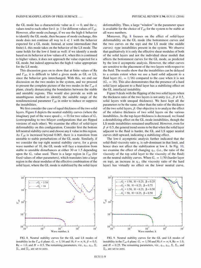
We first consider the case of equal thickness of the two solidlayers. Figure 8 depicts the neutral stability curves (where theimaginary part of the wave speed ci = 0) for two values of Gr

(corresponding to two bilayer configurations that are flippedversions of each other). We examine the effect of solid-layerdeformability on this configuration. Consider first the bottomleft neutral stability curve and choose any k value in this region.As �eff is increased beyond 0.065, there is a transition fromunstable to stable perturbations of the GL mode. Similarly, ifwe consider the top right neutral stability curve, for a givenwave number of 10, the GL mode will face a transition fromstable to unstable disturbances at either 30 or 1.5 dependingupon the Gr value used. There is a large region in �eff (forfixed values of other parameters), which translates into a largeregion in the shear modulus of the effective combination of thesolid layer, where the GL mode is stabilized by the solid-layer

10-3

10-2

10-1

100

101

Wave number, k

10-2

10-1

100

101

102

Γ eff

Gr = 1/16

Gr = 16

FIG. 8. Neutral stability curves for the GL and LS modes ofinstability in the �eff-k plane: Gr = 1/16 and 16, θ = π/4, β = 0.5,Re = 1.0, and H = 0.5. The remaining parameters, viz., ηr1, ηr2, , 1, and 2, are set to zero.

deformability. Thus, a large “window” in the parameter spaceis available for the choice of �eff for the system to be stable atall wave numbers.

Moreover, Fig. 8 focuses on the effect of solid-layerdeformability on the GL mode (the bottommost curves andthe two curves on the top) and the LS mode (the middlecurves) -type instabilities present in the system. We observethat qualitatively it is only the effective shear modulus of bothof the solid layers and not the individual shear moduli thataffects the bottommost curves for the GL mode, as predictedby the low-k asymptotic analysis. However, the other curvesare sensitive to the placement of the two layers with respect tothe fluid. The results show that the instabilities can be delayedto a certain extent when we use a hard solid adjacent to afluid layer (Gr = 1/16) compared to the case when it is not(Gr = 16). This also demonstrates that the presence of a hardsolid layer adjacent to a fluid layer has a stabilizing effect onthe GL interfacial instability.

Figure 9 deals with the flipping of the two solid layers whenthe thickness ratio of the two layers is not unity (i.e., β �= 0.5,solid layers with unequal thickness). We have kept all theparameters to be the same, other than the ratio of the thicknessof the two solid layers, β. Our objective is to analyze the effectof the relative thickness of two solid layers on the variousinstabilities. As the top-layer thickness is decreased, we founda destabilizing effect on the GL mode instabilities, though theLS mode instabilities remained unaffected. However, even forβ �= 0.5, the general trend seems to be that when the solid layeradjacent to the fluid is harder, the GL and LS upper neutralcurves shift upward, indicating a stabilizing effect.

The low-k asymptotic analysis further indicated that thesolid-fluid viscosity ratio ηr is sub-dominant in that limit, andhence does not affect the stabilization at low k. In Fig. 10,we examine the effect of changing ηr1 (i.e., the ratio of theviscosity of the top solid layer to the viscosity of the fluid)on the neutral stability curves. When Gr = 1/50 (harder layeron top), an increase in ηr1 (the viscosity ratio of the hardlayer) has virtually no effect on the lower neutral curve,

10-3

10-2

10-1

100

101

Wave number, k

10-2

10-1

100

101

102

Γ eff

Gr = 1/50, H = 0.25, β = 0.25

Gr = 50, H = 0.25, β = 0.75

Gr = 1/50, H = 0.25, β = 0.50

Gr = 50, H = 0.25, β = 0.50

FIG. 9. Neutral stability curves for the GL and LS modes ofinstability in the �eff-k plane: Gr = 1/50 and 50, θ = π/4, Re = 1.0,and H = 0.25. The remaining parameters, viz., ηr1, ηr2, , 1, and 2, are set to zero.

013111-9

SHIVAM SAHU AND V. SHANKAR PHYSICAL REVIEW E 94, 013111 (2016)

10-3

10-2

10-1

100

101

Wave number, k

10-2

10-1

100

101

102

Γ eff

Gr = 1/50, η

r1 = 0.1

Gr = 50, η

r1 = 0.1

Gr = 1/50, η

r1 = 0.0

Gr = 50, η

r1 = 0.0

FIG. 10. Neutral stability curves for GL and LS modes ofinstability in the �eff-k plane: Gr = 1/50 and 50, θ = π/4, Re = 1.0,H = 0.25, β = 0.5, ηr2 = 0, = 0, 1 = 0, 2 = 0, and differentηr1 values.

which was expected from asymptotic analysis. Interestingly,this increase only has a marginal stabilizing effect on theuppermost neutral stability curves. In contrast, when Gr = 50(softer layer on top), the change in viscosity ηr1 of the top layernow has a significant stabilizing effect on both of the upperneutral curves. Thus, an increase in the viscosity of the softerlayer further increases the gap between the lower and upperneutral curves, and hence increases the region where mode 1is completely suppressed. A similar trend is seen in Fig. 11,wherein the viscosity ηr2 of the bottom solid layer is increased,and even here, only the increase in the viscosity of the softerlayer has a significant stabilizing effect. This discussion thusshows that while the viscosity of either of the two solid layersdoes not have a destabilizing effect, the viscosity of the softerlayer (regardless of its placement) has a substantial stabilizingimpact on the upper neutral curves, and hence it increases thewindow of stability.

10-3

10-2

10-1

100

101

Wave number, k

10-2

10-1

100

101

102

Γ eff

Gr = 1/50, η

r2 = 0.1

Gr = 50, η

r2 = 0.1

Gr = 1/50, η

r2 = 0.0

Gr = 50, η

r2 = 0.0

FIG. 11. Neutral stability curves for GL and LS modes ofinstability in the �eff-k plane: Gr = 1/50 and 50, θ = π/4, Re = 1.0,H = 0.25, β = 0.5, ηr1 = 0, = 0, 1 = 0, 2 = 0, and differentηr2 values.

10-3

10-2

10-1

100

101

Wave number, k

10-2

10-1

100

101

102

Γ eff

Gr = 1/100, H = 0.25, β = 0.05

Gr = 1, H = 0.25

Gr = 1/50, H = 0.25, β = 0.05

FIG. 12. Neutral stability curves for GL and LS modes ofinstability in the �eff-k plane: Gr = 1/100 and 1/50, θ = π/4, Re =1.0, H = 0.25, β = 0.05, ηr1 = ηr2 = 0, and = 1 = 2 = 0.

We next consider the case of a very thin hard layer of solidthat is placed over a much thicker softer solid. Figure 12 showsthat if the parameters are chosen carefully, the free-surfaceinstability can be suppressed up to a large domain of �eff.As Gr is decreased (at a fixed β, thickness of the top layer),we find the upper neutral curves to shift upward, indicatinga strong stabilizing effect. This clearly demonstrates that theupper neutral curves are highly sensitive to the modulus of thesolid layer adjacent to the fluid, while the lower neutral curveis independent of those changes, and is a function only of theeffective modulus.

V. CONCLUSION

Previous studies have demonstrated that passive suppres-sion of free-surface and interfacial instabilities (which other-wise exist in flow past rigid surfaces) is possible by consideringa deformable solid layer lining over the rigid substrate ina variety of contexts. However, a major aspect of using adeformable solid layer is that new instabilities due to thedeformability of the solid layer could potentially proliferate,and hence it is necessary to have an accurate understandingof the window in the parameter space in which free-surfaceand other deformability-induced instabilities are suppressedat all wave numbers. In the present study, we proposed andevaluated the possibility of using a deformable “bilayer” solid,in which two solid layers, of different physical properties(elastic moduli, viscosity, and thickness) are sandwichedtogether, for the specific case of suppression of the free-surfaceinstability in flow down an inclined plane. Such a flow isknown to become unstable in flow down a rigid incline, anda key feature of this instability is that the flow is unstable inthe limit of long wavelengths. We carried out an asymptoticanalysis in the long-wave limit for free-surface flow past abilayer, which showed that the free-surface instability couldindeed be suppressed in the long-wave limit, and the parameterthat determines the suppression is the effective shear modulusof the bilayer, and not the individual shear moduli of thesolid layers. Thus, our asymptotic analysis shows that thesuppression of the instability is independent of the ordering

013111-10

PASSIVE MANIPULATION OF FREE-SURFACE . . . PHYSICAL REVIEW E 94, 013111 (2016)

of the two solid layers in the bilayer. Interestingly, the recentwork of Neelamegam et al. [26] showed that for single-layerplane Couette flow past a bilayer, the liquid-solid interfacialinstability depends on the specific bilayer configuration. Evenin the present case, as the solid is made sufficiently deformable,new instabilities (absent in flow down a rigid incline) appear,and these new instabilities do depend on the relative placementof the two solid layers.

The asymptotic result [Eq. (43)] can be used to providesome estimates on the values of physical parameters forwhich the present predictions could be realized in experiments.For a vertical plate, the asymptotic result predicts that9�effH > 6

5 Re for suppression of instability, which in terms ofdimensional parameters reduces to Geff < 15

2 η2H/ρR2. Usingη ∼ 10−1 Pa s, ρ ∼ 103 kg/m3, R ∼ 10−4 m, and H = 1/4,we obtain Geff < 2000 Pa. Upon using the expression forGeff and β = 0.05, we obtain G1 ∼ 105 Pa and G2 ∼ 103

Pa. Thus, the present predictions are expected to be validfor the flow of highly viscous liquid layers (with viscosity∼10−1 Pa s), of thickness in the range of 100 microns, withthe shear modulus of the hard and soft layers in the range105 and 103 Pa, respectively. We also carried out numericalcomputations at finite inertia and wave number to demonstratethat it is possible to choose the bilayer configuration (basedon relative placement, elastic moduli, thickness, and viscosity)in such a manner that the window of parameters in which thesystem is stable to perturbations of all wavelengths can besignificantly enhanced. Further, incorporation of dissipativeeffects in the solid showed that it is the viscosity of thesofter solid that leads to a substantial increase in the stablewindow, and that the viscosity of the harder layer does nothave a major impact on the stability. While this study hasfocused on the stability of flow down an inclined plane, weexpect that the qualitative trends would carry over to morecomplicated flows such as two-layer or core-annular flows withtwo immiscible fluids. Thus, deformable solid bilayers offersignificantly more options in the control and manipulation ofinterfacial instabilities in free-surface and multilayer flows.

APPENDIX A: WAVE SPEED FROMASYMPTOTIC ANALYSIS

In the asymptotic analysis, the complex wave speed can beexpanded in a series of k for k � 1. As discussed in Sec. III,it is sufficient to consider terms up to O(k) correction to wavespeed in the present study. Thus, the expansion of c leads to

c = c(0) + kc(1) + · · · . (A1)

We consider small perturbations in the present study in whichvz could be assumed to be of O(1), and using continuityequation (15) and x-momentum equation (16), we concludevx ∼ O(k−1) and p ∼ O(k−2), respectively. The expansion ofthe velocity and pressure in the liquid layer now are as follows:

vz = v(0)z + kv(1)

z + · · · , (A2)

vx = k−1v(0)x + v(1)

x + · · · , (A3)

p = k−2p(0) + k−1p(1) + · · · . (A4)

On a similar ground, the expansion of the dynamic quantitiesgoverning the dynamics of the upper solid layer, up to O(k)

consideration of uz1, could be expanded as

uz1 = u(0)z1 + ku

(1)z1 + · · · , (A5)

ux1 = k−1u(0)x1 + u

(1)x1 + · · · , (A6)

pg1 = k−2p(0)g1 + k−1p

(1)g1 + · · · . (A7)

Similarly, the displacements and pressure fields in the lowersolid layer are expanded as follows:

uz2 = u(0)z2 + ku

(1)z2 + · · · , (A8)

ux2 = k−1u(0)x2 + u

(1)x2 + · · · , (A9)

pg2 = k−2p(0)g2 + k−1p

(1)g2 + · · · . (A10)

Since the displacement fields in the solid layers are defined, thekinematic equation of the evolution of the free surface interfacefrom Eq. (27) dictates that the coefficient of the free-surfaceheight fluctuation can be expanded in a similar asymptoticseries in k:

h = k−1h(0) + h(1) + · · · . (A11)

To obtain the governing linearized equation in the liquid andsolid layers at the corresponding leading order and the firstcorrection, we substitute the series expansion of the perturbeddynamical quantities into the linearized equations for liquid,Eqs. (15)–(18), and for the two solid layers, Eqs. (19)–(22)and Eqs. (23)–(26), respectively. Similarly, the boundary andthe interface conditions at the leading order and O(k) couldbe obtained from substituting the expansion into Eqs. (27)–(39). We further divide this appendix into two subparts thatdeal with the sequential procedure of the calculations of theleading-order and O(k) dynamical quantities.

1. Leading-order dynamics

The governing equations for the leading-order velocity fieldv(0)

z in the liquid layer and the leading-order deformation fieldsu

(0)z1 and u

(0)z2 in the solid layers, as obtained from the asymptotic

series expansion, are

d4z v(0)

z = 0, (A12)

d4z u

(0)z1 = 0, (A13)

d4z u

(0)z2 = 0. (A14)

The leading-order boundary conditions at the free-surfaceinterface, z = 0, are

− 3h(0) + dzv(0)x = 0, (A15)

−p(0) = 0. (A16)

Similarly, the leading-order interface conditions at the fluid-solid interface, z = 1, are

v(0)z = 0, (A17)

v(0)x = 0, (A18)

dzv(0)x = 1

�1dzu

(0)x1 , (A19)

p(0) = p(0)g1 . (A20)

013111-11

SHIVAM SAHU AND V. SHANKAR PHYSICAL REVIEW E 94, 013111 (2016)

The interface conditions at the solid-solid interface at z =(1 + βH ) are

u(0)z1 = u

(0)z2 , (A21)

u(0)x1 = u

(0)x2 , (A22)

1

�1dzu

(0)x1 = 1

�2dzu

(0)x2 , (A23)

p(0)g1 = p

(0)g2 . (A24)

Lastly, the boundary conditions at z = (1 + H ) are

u(0)z2 = 0, u

(0)x2 = 0. (A25)

An important consequence of the low-wave-number expansionfor the interface conditions [Eqs. (30) and (31)] is that toleading order, the fluid velocities v(0)

z and v(0)x satisfy the no-

slip conditions at z = 1 as in a rigid boundary [Eqs. (A17)and (A18)]. This is because the right side of Eqs. (30) and (31)is O(k) smaller than the fluid velocities on the left side. Thisimplies that the solid-layer deformability does not influencethe leading-order fluid velocity field, and so the leading-orderwave speed in the present problem must be identical to that ofYih’s [15] analysis. However, the leading-order velocity fieldin the liquid layer exerts a shear stress on the solid layer viathe tangential stress condition [Eq. (A19)], and this causes adeformation in the solid layer at leading order. We now presentthe solution to the leading-order velocity and displacementfields, and the leading-order wave speed.

The analytical solution to the fourth-order differentialequation (A12) is given as

v(0)z = A1 + A2z + A3z

2 + A4z3. (A26)

Since this ordinary differential equation (ODE) is linear andhomogeneous in itself, the eigenfunction vz obtained from it isdetermined only to a multiplicative constant. Therefore, A1 =1 could be chosen without any loss of generality. Physically, wecan interpret this as the normalization of the amplitude of thenormal component of the leading-order liquid velocity at thefree surface by 1. The solutions to the leading-order dynamicalvariables of the liquid layer could be obtained by satisfyingthe leading-order boundary conditions [Eqs. (A16)–(A18)],

v(0)z = (z − 1)2, (A27)

v(0)x = 2i(z − 1), (A28)

p(0) = 0. (A29)

The free-surface height fluctuation at z = 0, to a leading order,could be found using Eq. (A16),

h(0) = 2i/3. (A30)

Therefore, the leading-order wave speed could be found usingthe linearized kinematic condition (27), and it is given as

c(0) = 3, (A31)

which matches Yih’s [15] result for liquid flow down aninclined rigid plane, as expected. Since the flow is neutrallystable to leading order, the stability of the system would bedetermined from the first correction to the wave speed. Wewould also be requiring the leading-order deformation in both

of the solid layers, and this could be obtained by solving thedifferential equations (A13) and (A14), whose solutions aregiven as

u(0)z1 = B1 + B2z + B3z

2 + B4z3, (A32)

u(0)z2 = C1 + C2z + C3z

2 + C4z3. (A33)

The multiplicative constants in the above solutions could be de-termined using the boundary conditions [Eqs. (A19)–(A25)].Finally, the leading-order deformation fields are given as

u(0)z1 = �1{z − (1 + βH )}2 (A34)

+ (1 − β)�2H {2 + (1 + β)H − 2z}, (A35)

u(0)x1 = 2i[�1{z − (1 + βH )} − �2H (1 − β)], (A36)

p(0)g1 = 0, (A37)

u(0)z2 = �2[z − (1 + H )]2, (A38)

u(0)x2 = 2i�2[z − (1 + H )], (A39)

p(0)g2 = 0. (A40)

With the calculation of the above leading-order dynamicalquantities, we now proceed to evaluate the first correction tothe wave speed c(1).

2. First correction to the wave speed

The O(k) equation obtained for the velocity field vz, whichrepresents the dynamics of v(1)

z , is

d4z v(1)

z = i Re[(vx − c(0))d2

z v(0)z − (

d2z vx

)v(0)

z

]. (A41)

The general solution to this inhomogeneous fourth-orderdifferential equation (A41) is given as

v(1)z = D1 + D2z + D3z

2 + D4z3 − i Re

20z5. (A42)

The multiplicative constant D1 must be set to zero sincepreviously we have fixed the amplitude of vz at z = 0 to be1 by setting the coefficient A1 at the leading order to be 1.The boundary conditions at z = 0 and 1, Eqs. (27)–(30), areused to determine the remaining three constant coefficients. Atthe free-surface interface z = 0, the continuity conditions fortangential and normal stress equations at order O(k) are

− 3h(1) + dzv(1)x = 0, (A43)

−p(1) − 3h(0) cot β = 0. (A44)

At the solid-liquid interface z = 1, the velocity continuityconditions at order O(k) are

v(1)z = −ic(0)u

(0)z1 , (A45)

v(1)x + dzvx |z=1u

(0)z1 = −ic(0)u

(0)x1 . (A46)

This coupling of liquid-solid at the interface gives rise to theO(k) velocity perturbation field, which is solely affected bythe leading-order deformation field in the upper solid layer.Using Eqs. (A44)–(A46), the O(k) component of the perturbedvelocity field is determined. The obtained solution for v(1)

z is

013111-12

PASSIVE MANIPULATION OF FREE-SURFACE . . . PHYSICAL REVIEW E 94, 013111 (2016)

as follows:

v(1)z = − iz

60{3 [60β2(�1 − �2)H 2 + 60�2H (2 + H − 2z)

− 120β(�1 − �2)H (−1 + z)

+ Re(−1 + z)2(−7 + 2z + z2)]

+ 20(−1 + z)2 cot β}.The inclusion of solid-layer deformation in the first correctionis through the terms that are proportional to �1 and �2. Thefirst correction to the height fluctuation h(1) obtained fromEq. (A43) is

h(1) = −4H [�1β + �2(1 − β)] + 815 Re − 4

9 cot β.

(A47)Finally, the linearized kinematic condition, Eq. (27), to O(k),given as

i[vx |z=0 − c(0)]h(1) − ic(1)h(0) = v(1)z |z=0, (A48)

is used to calculate the first correction to the wave speed c(1),

c(1) = i([

65 Re − cot β

] − 9H [�1β + �2(1 − β)]).

(A49)

APPENDIX B: CHARACTERISTIC EQUATION ATARBITRARY WAVE NUMBERS

In this appendix, we illustrate the numerical technique usedto solve the governing equations and boundary conditionsdescribed in Sec. II C. A shooting technique is implemented inwhich an initial guess of the solution (c, here) is provided, andwith the help of the Newton-Raphson method, the final valueof the iterated eigenvalue is obtained after following sufficientiterations so as to meet the suitable convergence criterion. Thismethod of numerical integration is very common in the linearstability analysis, and therefore the solution methodology hasbeen adopted from [12,13]. A brief explanation of the codingprocedure is further explained here: The governing equationsfor the liquid and solid layers can be recast into respectivesingle fourth-order ordinary differential equations (ODEs).Therefore, we have three fourth-order ODEs governing vz forliquid and uz1 and uz2 in the solid layers. These three fourth-order ODEs along with boundary conditions completelyspecify the eigenvalue problem, the parameter c (complex

wave speed) being the eigenvalue. The numerical code forarbitrary Re uses the fourth-order Runge-Kutta integrator witha uniform step-size control to numerically integrate the ODEs,and a Newton-Raphson technique to find the solution of acharacteristic equation. We first started from the lower solidlayer and we began moving toward the free surface of the liquidlayer. To carry this out, we must specify “initial conditions”for the function uz2 and its first three derivatives at a givenvalue of the independent variable z. For the lower solid layerat z = (1 + H ), we have the zero displacement conditionsuz2 = 0 and ux2 = i

kdzuz2 = 0. We use two different (linearly

independent) sets of higher derivatives, d2z uz2 = (1,0) and

d3z uz2 = (0,1), at z = (1 + H ) and we numerically integrate

the differential equation (26) up to z = (1 + βH ). This yieldstwo linearly independent solutions to the displacement fieldconsistent with the two zero displacement conditions at z =(1 + H ) in the solid layer. Corresponding to these two linearlyindependent solutions, we evaluate the displacement field ofthe upper solid layer uz1 and its higher derivatives [whichwill be acting as the initial guesses for the shooting methodwhile integrating the fourth-order differential equation in theupper solid layer ranging from z = (1 + βH ) to z = 1] fromthe interfacial conditions at z = (1 + βH ) [Eqs. (34)–(37)].Using these two sets of values of uz1 acting as initial guesses,we now numerically integrate the fourth-order differentialequation (22) from z = (1 + βH ) to z = 1. After applying theinterface conditions [Eqs. (30)–(33)], we obtain the velocityfield vz and its higher derivatives in the liquid layer at z = 1,which again will be acting as the initial guesses for integratingthe fourth-order differential equation (18). Using these twosets of values for vz and its derivatives as the initial guesses,we integrate the Orr-Sommerfeld equation (18) for the fluidstarting from z = 1 to the free surface at z = 0. The velocityfield in the fluid is obtained as a linear combination of thesetwo solutions. At z = 0, the fluid velocity field must satisfy thefree-surface conditions (28) and (29). This is written in matrixform, and the determinant of this matrix is set to zero to obtainthe characteristic equation. This is solved numerically using aNewton-Raphson iteration procedure to obtain the eigenvaluec, for species values of �eff, Re, k, β, H, , 1, 2, ηr1, andηr2. We use the low-k asymptotic results as a starting guessfor the numerical procedure, and we continue with the low-kresults numerically to finite values of k.

[1] T. W. Kao, Role of viscosity stratification in the instability oftwo-layer flow down an incline, J. Fluid Mech. 33, 561 (1968).

[2] D. S. Loewenherz and C. J. Lawrence, The effect of viscositystratification on the stability of a free surface flow at lowReynolds number, Phys. Fluids A 1, 1686 (1989).

[3] C. Pozrikidis, Instability of multilayer channel and film flows,Adv. Appl. Mech. 40, 179 (2004).

[4] K. P. Chen, The onset of elastically driven wavy motion in theflow of two viscoelastic liquid films down an inclined plane,J. Non-Newtonian Fluid Mech 45, 21 (1992).

[5] Y. Renardy, Stability of the interface in two-layer Couette flowof upper convected Maxwell liquids, J. Non-Newtonian FluidMech. 28, 99 (1988).

[6] K. P. Chen, Wave formation in the gravity-driven low-Reynoldsnumber flow of two liquid films down an inclined plane, Phys.Fluids A 5, 3038 (1993).

[7] W. Y. Jiang, B. Helenbrook, and S. P. Lin, Inertialess insta-bility of a two-layer liquid film flow, Phys. Fluids 16, 652(2004).

[8] W. Y. Jiang and S. P. Lin, Enhancement or suppression ofinstability in a two-layered liquid film flow, Phys. Fluids 17,054105 (2005).

[9] A. S. Utada et al., Monodisperse double emulsions generatedfrom a microcapillary device, Science 308, 537 (2005).

[10] A. S. Utada et al., Dripping, jetting, drops, and wetting: Themagic of microfluidics, MRS Bull. 32, 702 (2007).

013111-13

SHIVAM SAHU AND V. SHANKAR PHYSICAL REVIEW E 94, 013111 (2016)

[11] S. P. Lin, J. N. Chen, and D. R. Woods, Suppressionof instability in a liquid film flow, Phys. Fluids 8, 3247(1996).

[12] V. Shankar and L. Kumar, Stability of two-layer Newtonianplane Couette flow past a deformable solid layer, Phys. Fluids16, 4426 (2004).

[13] V. Shankar and A. K. Sahu, Suppression of instability in liquidflow down an inclined plane by a deformable solid layer, Phys.Rev. E 73, 016301 (2006).

[14] A. Jain and V. Shankar, Instability suppression in viscoelasticfilm flows down an inclined plane lined with a deformable solidlayer, Phys. Rev. E 76, 046314 (2007).

[15] C.-S. Yih, Stability of liquid flow down an inclined plane, Phys.Fluids 6, 321 (1963).

[16] C.-S. Yih, Instability due to viscosity stratification, J. FluidMech. 27, 337 (1967).

[17] V. Kumaran, G. H. Fredrickson, and P. Pincus, Flowinduced instability of the interface between a fluid and a gelat low Reynolds number, J. Phys. II 4, 893 (1994).

[18] L. Landau and E. Lifshitz, Theory of Elasticity (Pergamon, NewYork, 1989).

[19] V. Gkanis and S. Kumar, Instability of creeping Couette flowpast a neo-Hookean solid, Phys. Fluids 15, 2864 (2003).

[20] V. Gkanis and S. Kumar, Stability of pressure-driven creepingflows in channels lined with a nonlinear elastic solid, J. FluidMech. 524, 357 (2005).

[21] L. E. Malvern, Introduction to the Mechanics of a ContinuousMedium (Prentice-Hall, Englewood Cliffs, NJ, 1969).

[22] G. A. Holzapfel, Nonlinear Solid Mechanics (Wiley, Chichester,UK, 2000).

[23] V. Gkanis and S. Kumar, Instability of gravity-driven free-surface flow past a deformable elastic solid, Phys. Fluids 18,044103 (2006).

[24] Gaurav and V. Shankar, Stability of gravity-driven free-surfaceflow past a deformable solid layer at zero and finite Reynoldsnumber, Phys. Fluids 19, 024105 (2007).

[25] V. Gkanis and S. Kumar, Instability of creeping flow past adeformable wall: The role of depth-dependent modulus, Phys.Rev. E 73, 026307 (2006).

[26] R. Neelmegam, D. Giribabu, and V. Shankar, Instability ofviscous flow over a deformable two-layered gel: Experimentand theory, Phys. Rev. E 90, 043004 (2014).

013111-14