Embed Size (px)
Citation preview
UNIVERSIDAD TECNICA FEDERICO SANTA MARIA
DEPARTAMENTO DE ELECTRONICA
PASSIVITY BASED CONTROL OF IRREVERSIBLEPORT HAMILTONIAN SYSTEM: AN ENERGY
SHAPING PLUS DAMPING INJECTIONAPPROACH
Tesis de Grado presentada por
Ignacio Villalobos Aguilera
como requisito parcial para optar al tıtulo de
Ingeniero Civil Electronico
y al grado de
Magıster en Ciencias de la Ingenierıa Electronica
Profesor GuıaDr. Hector Ramırez Estay
Valparaıso, 2020.

TıTULO DE LA TESIS:
PASSIVITY BASED CONTROL OF IRREVERSIBLE PORT HAMIL-TONIAN SYSTEM: AN ENERGY SHAPING PLUS DAMPINGINJECTION APPROACH
AUTOR:
Ignacio Villalobos Aguilera
TRABAJO DE TESIS, presentado en cumplimiento parcial de los requisitos para el tıtulode Ingeniero Civil Electronico y el grado de Magıster en Ciencias de la Ingenierıa Electronicade la Universidad Tecnica Federico Santa Marıa.
Dr. Hector Ramırez E.
Dr. Daniel Sbarbaro H.
Dr. Juan Yuz E.
Valparaıso, 31 Agosto de 2020.


dedicado a mi tıa
a mi brujita
a mi pichonga
y a mi lelita
las amo por siempre.


ACKNOWLEDGMENTS
Creo que esta es la parte mas difıcil de escribir de esta tesis. Hay tanta gente que meinfluencio en mi paso por la tan hermosa etapa universitaria; primero que nada gracias a mifamilia; gracias por apoyarme en mi capricho de querer estudiar electronica en Valparaıso,pues nuestras condiciones economicas quizas no lo permitıan. Independiente de donde meencuentre o donde termine en el futuro, las llevo conmigo siempre.
Gracias a todos mis amigos; a mis compas de plan comun, que a pesar de que todosterminamos en cosas distintas, no perdemos el contacto hasta hoy; a mis amigos en Valpito:hago menciones especiales a Dauros y al tim, amigos de muchas noches de laboratorios,tareas, informes y de bohemia; gracias por ayudar a este ‘guacho humilde’ economicamentesiempre que lo necesite. Esas son cosas que no se olvidan nunca; gracias a Ivan, que en lapension aguantabamos semanas de tallarines; gracias a Claudia por haber sido un apoyofundamental estos ultimos meses. Eres una personita maravillosa.
Gracias a todos los profesores y profesoras que tuve; de algunos aprendı mas y de otrosmenos, pero todos aportaron un granito de arena a mi formacion: hago mencion especiala los profesores Juan Yuz, Milan Derpich, Juan Carlos Aguero y Hector Ramırez por suexcelente calidad academica y humana.
A mi profesor guıa Hector Ramırez. Estimado profesor, muchas gracias por este ano ymedio de trabajo juntos, gracias por aguantar ese mal habito mio de dejar muchas cosaspara el dıa anterior; y gracias por escucharme en muchas ocasiones que no estaba bien. Notengo nada mas que buenas palabras para usted, tanto en lo academico como en lo humano.A usted y a Giss les deseo felicidad por siempre.
Durante la U aprendı mucho menos de lo que deberıa haber aprendido, pero mucho masde lo que me imagine aprender nunca; estoy satisfecho.
Este trabajo fue hecho en el contexto de los proyectos FONDECYT regular 1191544 yBasal FB0008.
i


CONTENTS
ACKNOWLEDGMENTS i
RESUMEN v
ABSTRACT vii
1 INTRODUCTION 11.1 Motivation and state of the art 11.2 Organization of the chapters of this thesis 21.3 Main Contributions 3
2 REVERSIBLE-IRREVERSIBLE PORT HAMILTONIAN SYSTEMS 42.1 Port Hamiltonian Systems - PHS 4
2.1.1 The PHS formulation 42.1.2 A key property: the Casimir functions 52.1.3 Example: The MSD system 62.1.4 Casimir functions of the MSD system 7
2.2 Irreversible Port Hamiltonian Systems - IPHS 72.2.1 The IPHS formulation 82.2.2 Example: The IPHS model of the CSTR system 82.2.3 The Coupled PHS-IPHS formulation 102.2.4 Casimir functions for Coupled PHS-IPHS 112.2.5 Example: non-isothermal RLC system 112.2.6 Casimir functions of the non-isothermal RLC system 13
3 PASSIVITY BASED CONTROL METHODS APPLIED TO IPHS 143.1 Passivity Based Control of PHS 14
3.1.1 Lyapunov Stability Theorem 143.1.2 Lasalle’s Invariance Principle 153.1.3 Control by Interconnection of PHS 153.1.4 Damping injection 173.1.5 Example: Cbi-Di for the MSD system 18
3.2 Passivity Based Control of IPHS 193.2.1 Control by interconnection of IPHS 203.2.2 Damping Injection 233.2.3 Cbi-Di control of the CSTR system 25
iii
iv Acknowledgments
4 A CASE STUDY: THE GAS-PISTON SYSTEM 294.1 Coupled PHS-IPHS model of the Gas-Piston system 29
4.1.1 Cbi-Di control of the Gas-Piston system 314.2 Numerical Simulations 34
4.2.1 Simulated Cases 344.2.2 Simulation Values 354.2.3 Simulation Results 35
5 CONCLUSION 405.1 Future Work 40
REFERENCES 41
RESUMEN
Los sistemas puerto Hamiltonianos irreversibles (IPHS) son una extension de la clasicaformulacion de sistemas puerto Hamiltonianos (PHS). Al igual que los sistemas PHS, estaforma de modelado permite representar una gran cantidad de sistemas multifısicos, conla capacidad de representar cada sistema fısico como un bloque capaz de conectarse conlos demas a traves de funciones de energıa. A diferencia de un sistema PHS, los IPHSrepresentan en su estructura el primer principio de la termodinamica (conservacion de laenergıa) y el segundo principio termodinamico (la creacion irreversible de entropıa). Estarepresentacion pues, permite no solo el modelado de sistemas electromecanicos sino quetambien permite representar a sistemas termodinamicos y en general, sistemas con procesosirreversibles. Este formalismo, al igual que en sistemas PHS, provee un marco teorico parael control de sistemas multifısicos.
Tecnicas de control pasivas y no lineales han demostrado ser utiles en el control desistemas PHS. Estas tecnicas tienen como objetivo modificar la funcion de energıa del sistemade forma tal que la funcion de energıa resultante sea un candidato a funcion de Lyapunov,y tenga un mınimo estricto de energıa en un punto de equilibrio deseado. Esta forma decontrol garantiza la estabilizacion del sistema en un punto de equilibrio deseado, junto conla estabilidad asintotica del sistema.
Dentro de estas tecnicas de control pasivas, control por interconeccion y modelado deenergıa han sido utilizadas para cambiar el punto de equilibrio de una funcion de energıacandidata a funcion de Lyapunov en sistemas PHS; la existencia y utilizacion de las funcionesde Casimir resultan, por lo tanto, fundamentales para tal proposito pues estas funcionesson invariantes estructurales del sistema. Si bien la estabilidad del sistema es garantizadamediante control por interconexion, la incorporacion adicional de amortiguacion, a travesde la entrada pasiva del sistema, asegura que el sistema sea asintoticamente estable en elpunto deseado.
El principal objetivo de esta tesis es extender las tecnicas de control pasivas y no lin-eales utilizadas en sistemas PHS al control de sistemas IPHS. En particular, se propone unmetodo sistematico de diseno de controladores para IPHS, basado en las tecnicas de controlpor interconexion y la inyeccion de amortiguamiento. Para ello, se plantea una estructurade controlador IPHS como interconexion con el sistema, y se derivan condiciones para laexistencia de invariantes estructurales que permitan mover el punto de equilibrio. En elproceso de diseno, resulta de gran importancia para el diseno de la funcion de energıa, elconcepto de funcion de disponibilidad. Esta funcion resulta ser un candidato a funcion deLyapunov para un punto de equilibrio deseado, y estrictamente convexa.
El resultado es un metodo sistematico de diseno, haciendo uso de las tecnicas clasicas decontrol pasivo como control por interconexion y energy shaping, junto con invariantes estruc-
v

vi Resumen
turales de Casimir, y funciones de disponibilidad de energıa; para sintetizar un controladorque estabiliza el sistema IPHS en un equilibrio dinamico deseado, y que es asintoticamenteestable. Finalmente, se realizan simulaciones utilizando sistemas con procesos irreversibles-reversibles.
ABSTRACT
Irreversible Hamiltonian Port Systems (IPHS) are an extension of the classic Port Hamil-tonian System (PHS) Formulation. Like PHS systems, this form of modeling allows therepresentation of a large number of multiphysical systems, with the ability to representeach physical system as a block capable of connecting with the others through energy func-tions. Unlike a PHS system, IPHS represent in their structure not only the first principle ofthermodynamics (energy conservation) but also the second thermodynamic principle (theirreversible creation of entropy). Therefore, this representation allows not only the modelingof electromechanical systems but also allows to represent thermodynamic systems and, ingeneral, systems with irreversible processes. This formalism provides. as in the case of PHS,a theoretical framework for the control of multiphysical systems.
Passive and non-linear control techniques have proven to be useful in controlling PHSsystems. These techniques aim to modify the energy function of the system such that theresulting energy function is a candidate for a Lyapunov function, and has a strict minimumenergy at a desired equilibrium point. This form of control ensures stabilization of thesystem at a desired equilibrium point, along with asymptotic stability of the system.
Within these passive control techniques, control by interconnection and energy shapinghave been used to change the natural equilibrium point of a Lyapunov candidate energyfunction in PHS; the existence and use of the Casimir functions are, therefore, fundamentalfor this purpose since these functions are structural invariants of the system. Althoughthe stability of the system is guaranteed by the energy-Casimir control, the additionalincorporation of damping, through the passive input of the system, ensures that the systemis asymptotically stable at the desired point.
The main objective of this thesis is to extend the passive and non-linear control tech-niques used for PHS to the control of IPHS. Precisely, a systematic design method controlfor IPHS is proposed, based on control by interconnection techniques and damping injection.For this, an IPHS controller structure is proposed as an interconnection with the system,and conditions are derived for the existence of structural invariants that allow changing theequilibrium point. In the design process, the concept of availability function is of greatimportance for the design of the energy function. This function turns out to be a candidatefor a Lyapunov function for irreversible systems.
The result is a systematic design method, using classical passive control techniques suchas control by interconnection and energy shaping, along with Casimir structural invariants,and energy availability functions to synthesize a controller that stabilizes the IPHS systemin a specified dynamic equilibrium, and that is asymptotically stable. Finally, simulationsare performed using systems with irreversible-reversible processes.
vii


Chapter 1
INTRODUCTION
In this introductory chapter, the port Hamiltonian framework is recalled; we give the stateof the art in the passivity based control techniques for the control of PHS. Subsequently, wemention extensions for the PHS framework to cope with systems that come from irreversiblethermodynamics, as PHS are used for modelling and control of electromechanical systems inits classic definition. One of these extension is called irreversible port Hamiltonian systems(IPHS) which can be used to model multiphysical systems and therefore its definition canbe exploited for control purposes.
The organization of the chapters and the main contributions of this thesis are also given.
1.1 Motivation and state of the art
The Port Hamiltonian system formulation (PHS) has been used for control and modellingof electrical, mechanical, and in general multiphysics systems ([22], [10], [36]) which aredescribed by the first law of thermodynamic. The PHS framework formalizes the basicinterconnection laws, e.g Kirchhoff laws in electrical systems or Newton laws in mechanicalsystems, together with the power preserving elements by a geometric structure using theenergy between the elements as the interconnection, and defines the Hamiltonian as thetotal energy stored in the system.
Energy then becomes essential in modeling systems as PHS, since it relates variables thatcome from different physical domains. Since the PHS framework is defined by a Hamiltonianenergy function of its power preserving elements, it has been largely used for the control ofmultiphysical domain systems ([36], [10]).
A key property for the control of PHS is the existence of the Casimir functions ([37],[10], [38]) which are structural invariants of the system.
Control by interconnection (Cbi) techniques aim at closing the PHS system in aloop with negative feedback, and with a controller that also has a PHS structure. In thisway, the total energy of the system is represented by the sum of the energies of the controllerand the PHS system. The controller energy is designed in such a way that the total energy ofthe system is a candidate for Lyapunov function and has a global minimum at some desiredequilibrium point ([25],[27],[37]). By Casimir generation, the coordinates of the system arerelated to the Casimir function and the useful Casimir functions for the closed-loop systemsatisfy a set of partial differential equations (PDE) [37].
A proper choice of an energy controller function such that the Hamiltonian for theclosed-loop system is a candidate Lyapunov function, guarantees stability of the systemat the equilibrium point [37], while the asymptotic stability of the system is achieved bythe injection of damping (Di). A generalization of the energy-Casimir method is the
1
2 CHAPTER 1. INTRODUCTION
interconnection and damping assignment passivity based control (IDA-PBC)which has been developed in [26]. In the IDA-PBC control method, the closed-loop energyfunction is obtained directly through the resolution of a set of partial differential equations,through the choice of a desired controller and damping. Unlike control by interconnection,in IDA-PBC the energy is obtained directly from the resolution of a PDE, and not bycompleting squares or some other tentative method.
Port Hamiltonian system theory, as mentioned at the beginning of the section, hasbeen successfully used for modeling electromechanical systems; that is, systems that can bemodeled by the first principle of energy conservation, but fails (in its classical definition)to model systems that express in their behavior the second principle of thermodynamics.Various authors have proposed extensions to the PHS theory, to encompass system whicharise from irreversible phenomena.
The framework of GENERIC was first developed in the work of ([14], [29], [28]) toencompass both reversible and irreversible physical systems for isolated thermodynamicssystems. Later in the work of ([23], [20]) the framework was extended to open systems.
In ([9], [5]) a representation of PHS which are called pseudo Hamiltonian was devel-oped to represent a large class of dynamical systems, and furthermore in [6] the frameworkwas used for the study of the stability of dynamical systems.
The papers ([11], [12]) define the control contact systems, generalizing the input-output port Hamiltonian systems to cope with models derived from irreversible thermody-namics.
A recent framework to encompass systems which have reversible-irreversible phenomenawas developed in [32], namely Irreversible port-Hamiltonian systems (IPHS). Thesesystems express as a structural property the first and second principles of thermodynamicsby adding a non linear real function to the dynamics. By definition, IPHS are non-linearsystems with a physically meaningful structure and just as PHS systems, they are definedwith respect to the total energy stored in the system. This approach makes it possible tointerconnect them with other reversible or non-reversible systems, or a combination of both[33]. Some first approaches to control of IPHS have been given in [31] using an IDA-PBClike approach, with the framework of an energy based availability function as a candidatefor a Lyapunov function, which is based in the spirit of the works of [1] and [39].
The purpose of this thesis is to extend the passive and non-linear techniques to thecontrol of IPHS, proposing a systematic design method for the control of irreversible portHamiltonian systems, based on control by interconnection plus damping injection (Cbi-Di),altogether with the availability function.
1.2 Organization of the chapters of this thesis
This thesis is divided into five chapters.
• Chapter 2 : A brief review of port Hamiltonian systems (PHS) is given along withtheir main characteristics such as the existence of invariants structures called Casimirfunctions. The PHS model of a Mass-Spring-Damper system is also shown as anexample and Casimir functions for this system are obtained.
The definition and properties of the Irreversible port Hamiltonian systems (IPHS) areshown, and how in their non-linear structure, they are capable of capturing the secondlaw of thermodynamics; the existence of Casimir functions for this framework is shown.We give the example of a non isothermal RLC system, which can be seen as a coupled
1.3. MAIN CONTRIBUTIONS 3
PHS-IPHS and we obtain its Casimir functions. The example of a Continuous StirredTank Reactor (CSTR) system is also given, which can be modelled as a pure IPHS.
• Chapter 3 : In this chapter, the control by interconnection plus damping injection(Cbi-Di) of PHS systems is reviewed; the Lyapunov stability theorem and the invari-ance principle are recalled, as they are fundamental to the theory. A Cbi-Di controlleris obtained for the Mass-Spring-Damper system as an example.
Subsequently, the Cbi-Di control is extended to IPHS. A systematic control designmethod for IPHS is shown, specializing the control by interconnection and dampinginjection to IPHS.
The IPHS model of the CSTR is used to synthesize a Cbi-Di controller for a generalreaction of m species.
• Chapter 4 : The IPHS model of a Gas-Piston system is derived; a Cbi-Di controlleris then obtained using the framework of the Cbi-Di control for IPHS.
The Cbi-Di controller is then simulated using Matlab-Simulink to show the perfor-mance of the controller.
• Chapter 5 : Conclusions and comments about future work are given in this chapter.
1.3 Main Contributions
The main contributions of this thesis can be summarized in the following points:
• The framework of the control by interconnection plus damping injection (Cbi-Di) isextended to IPHS systems providing a systematic control design method for IPHS.
• The synthesis of an IPHS controller for a CSTR is given and it is shown that itcoincides with a controller obtained using an IDA-PBC type of design.
• A Gas-Piston system is used as case study; a Cbi-Di controller is designed and simu-lations are provided to evaluate different performances.
Chapter 2
REVERSIBLE-IRREVERSIBLEPORT HAMILTONIAN
SYSTEMS
This chapter recalls the definition of a port Hamiltonian system, along with its main char-acteristics and properties. As an example, the PHS model of the classic mechanical Mass-Spring-Damper system is obtained.
In the second part, the definition of an irreversible port Hamiltonian system is presented;its main properties are analyzed, and the main differences with the definition of a PHSsystem. As an example of the framework, the IPHS models of two systems are shown: anon-isothermal RLC system, which is a system with reversible-irreversible phenomena anda CSTR chemical reactor which is a purely irreversible system.
2.1 Port Hamiltonian Systems - PHS
The framework of port-Hamiltonian system (PHS) arise from the first principle of the ther-modynamic and its application to complex multiphysical systems ([36], [37]). The port-Hamiltonian system theory formalizes the basic interconnection laws together with the powerpreserving energy-storing elements by a geometric structure, using the Hamiltonian func-tion as the total energy of the system ([25], [27], [37], [35]). This approach has been used tomodel complex and multiphysical system since energy serves as the lingua franca betweenthe systems.
2.1.1 The PHS formulation
Definition 1. An input/state output/port PHS is defined by the dynamical equation
x(t) = [J(x)−R(x)]∂H
∂x+ g(x)u(t)
y(t) = g>(x)∂H
∂x
(2.1.1)
where x(t) ∈ <n is the state space vector, u(t) ∈ <m is the input of the system, H(x) : <n →< is the Hamiltonian energy function and g(x) ∈ <n×m is the input map. The matricesJ(x) ∈ <n×n, R(x) ∈ <n×n are respectively, the structure matrix and the dissipation matrixof the system which satisfy J = −J> and R = R> ≥ 0. The interconnection matrix J(x)
4
2.1. PORT HAMILTONIAN SYSTEMS - PHS 5
by its skew-symmetric property is power conserving. The resistive matrix R(x), by its nonnegative property express the internal dissipation energy of the system.
The energy balance equation of the function H(x) express the first principle of thethermodynamics. Taking the time derivative of the energy function
dH
dt=dH>
dx
dx
dt
= −dH>
dxRdH
dx+dH>
dxgu
= −dH>
dxRdH
dx+ y>u ≤ u>y (2.1.2)
because R ≥ 0 and where u>y is an external supply power; inequality (2.1.2) shows that thePHS cannot store more energy than the one supplied from the external port. Now, considerthe following definition.
Definition 2 ([21]). The Poisson bracket is defined with respect to a constant skew-symmetric matrix J = −J>, acting on any two smooth functions Z,G as
Z,GJ =∂ZT
∂x(x)J
∂G
∂x(x) (2.1.3)
The structure matrix J not only represents the energy flow between different physicalsystems domains, but it is also related to a simpletic structure called Poisson bracket (Def-inition 2) which is also skew symmetric due to the structure matrix J . If J is a Poissonstructure, then it satisfies the integrability conditions which are refered as Jacobi identities[37]. The properties of the Poisson bracket implies the existence of energy conservationlaws as they define conserved quantities. As we shall see in the next chapter, the energyconservation is fundamental in the passivity based control techniques (PBC).
The dynamical equations of the PHS, with dissipation matrix R = 0, can be written interms of the Poisson bracket as
dx
dt= x, UJ + g(x)u(t)
2.1.2 A key property: the Casimir functions
A key property of the PHS framework is the existence of structural invariants. Let usconsider a real function C and let us explore the equation
∂C>
∂x(J(x)−R(x)) = 0 (2.1.4)
Suppose that equation (2.1.4) has a solution. From the time derivative of C along thetrajectories of the port Hamiltonian system (Definition 1), it follows
dC
dt=∂C>
∂x
[(J −R)
∂H
∂x+ gu
]=∂C>
∂xgu (2.1.5)
If we set u = 0, the function C(x) remains constant along the trajectories of the PHS,
with no dependency of the Hamiltonian function H. Furthermore, if ∂C>
∂x g = 0 then theinvariance holds for any input u. Functions C(x) that satisfy equation (2.1.4) are calledCasimir functions of the system and its existence has implications on the stability analysisof a PHS system ([37], [36], [25], [27], [35]). Consider then the following definition.
6 CHAPTER 2. REVERSIBLE-IRREVERSIBLE PORT HAMILTONIAN SYSTEMS
Figure 2.1. Mass Spring Damper system.
Definition 3 ([37]). A Casimir function for an input-output port PHS (Definition 1) isany function C(x) : <n → < which satisfies
∂C>
∂x(J(x)−R(x)) = 0 (2.1.6)
Furthermore, as it was shown in (2.1.5), by setting u = 0 then
dC
dt= 0
Thus, the Casimir function is a conserved quantity of the system for u = 0, independently
of the Hamiltonian H. If ∂C>
∂x g = 0 then the invariance holds for any input u.
The previous results on the Casimir function can be summarized in the next proposition
Proposition 1 ([37]). The function C(x) : <n → < is said to be a Casimir function forthe PHS in Definition 1 if and only if
∂C>
∂xJ(x) = 0,
∂C>
∂xR(x) = 0, x ∈ <n (2.1.7)
As we see, the Casimir functions act as invariant structures for a PHS system. Thisdefinition is fundamental in PBC techniques which aim at shaping the Hamiltonian energyfunction. Next we give as an example of the PHS modeling the mass-spring-damper system.
2.1.3 Example: The MSD system
As an illustrative example, we consider the classical benchmark of the mass-spring-damperwhich is a mechanical system with dissipation. Let us consider Figure 2.1; the PHS formu-lation of the MSD is done following the Newton’s second law:
Mq = F − kq − f q
2.2. IRREVERSIBLE PORT HAMILTONIAN SYSTEMS - IPHS 7
where q is the relative position of the system. The term kq is the force of the spring actingon the mass M which is proportional due to Hooke’s law; the term f q is the force of thedamper acting on the mass. The Hamiltonian energy of the system is then
H(q, p) = kq2
2+
p2
2M
Where p is the momentum of the system. The MSD system has the PHS form
x =
(qp
)=
([0 1−1 0
]−[0 00 f
])(kqq
)+
(01
)F
y =(0 1
)(kqq
)= q
(2.1.8)
where the structure matrix J of the system, the dissipation matrix and the input map are,respectively
J =
[0 1−1 0
], R =
[0 00 f
], g =
(01
)The structure matrix J satisfies the skew-symmetric property J = −J> and the dissipationmatrix is such that R = R> ≥ 0 verifying the non-negative condition.
2.1.4 Casimir functions of the MSD system
Let us explore for Casimir functions of the system (2.1.8) by setting u = 0. By Proposition1 we take C(q, p) : <2 → < such that the system of partial differential equations (PDE)
∂C>
∂xJ(x) = 0
∂C>
∂xR(x) = 0
hold for every x = (q, p) ∈ <2; note that ∂C>
∂x =(∂C∂q
∂C∂p
). The Casimir function then has
to satisfy ∂C∂q = ∂C
∂p = 0 with solution C = k ∈ < being any real constant; which shows thatthere are not non trivial Casimir functions for the MSD system.
2.2 Irreversible Port Hamiltonian Systems - IPHS
The irreversible port Hamiltonian systems have been proposed in [32] and [33] as an exten-sion of the port Hamiltonian system framework. IPHS encompass systems arising from theirreversible thermodinamics by expressing as a structural property not only the first thermo-dynamical principle, which is associated with the energy conservation, but also the secondthermodynamical principle, which is associated with the irreversible creation of entropy. Inthis section, we give the classic IPHS definition proposed in [32]; this definition encompassessystems that express purely irreversible phenomena. Further, the extended IPHS definition([33]) is given, which encompasses systems with reversible-irreversible phenomena.
8 CHAPTER 2. REVERSIBLE-IRREVERSIBLE PORT HAMILTONIAN SYSTEMS
2.2.1 The IPHS formulation
Definition 4 ([32]). An IPHS is defined by the dynamical equations
x = J(x, ∂U∂x
) ∂U∂x
+ g(x, ∂U∂x
)u
y = g(x, ∂U∂x
)> ∂U∂x
(2.2.1)
where x(t) ∈ <n is the state space vector, u(t) ∈ <m is the input of the system, U(x) :<n → < is the Hamiltonian energy function which is a smooth function of the state x. Thestructure skew-symmetric matrix is J = −J> and the input map is g ∈ <n×m. There existsa smooth entropy function S(x) : <n → <. The non-linear modulating function R is definedas
R(x, ∂U∂x
)= γ
(x, ∂U∂x
)S,UJ (2.2.2)
where γ(x, ∂U∂x
): <n → < is such that γ ≥ 0,i.e, a non linear positive function.
Let us see the balance equations of the energy function U(x) and entropy function S(x)which express respectively, the conservation of the energy and the irreversible creation ofentropy. In effect, taking the time derivative of the energy function
dU
dt= R
dUT
dxJdU
dx+dUT
dxgu
= y>u
where U,UJ = dUT
dx JdUdx = 0 due to the skew-symmetry of the structure matrix J ; which
express that the IPHS is a lossless dissipative system with supply rate y>u. Now taking thetime derivative of the entropy like function S(x) and setting u = 0 for simplicity, we get
dS
dt= R
dS>
dxJdU
dx
= γ(x, ∂U∂x
)S,U2J = σ ≥ 0
where σ is the internal entropy production and it shows that the entropy is an increasingfunction of x and always positive.
As we see in Definition 4, the main difference with the PHS definition lies in the modu-lating function R(x). In [32],[33] it has been seen that in fact, for thermodynamics systems,J is a matrix whose elements are 1, 0,−1 and which is associated with the structure ofthe IPHS. Thus represent the energy flow between different physical systems domains; themodulating function R then captures the dynamical behavior of the system. Definition 4is useful when one is modeling pure irreversible systems. In the next section we give theexample of a CSTR system which can be modelled as an IPHS exploiting Definition 4.
2.2.2 Example: The IPHS model of the CSTR system
In this section we present, as an example, a continuous stirred tank reactor (CSTR), whichis a system that can be interpreted within the framework of IPHS.
Let us consider a CSTR system with the following reversible reaction scheme:
m∑i=1
ζiAir
m∑i=1
ηiAi (2.2.3)

2.2. IRREVERSIBLE PORT HAMILTONIAN SYSTEMS - IPHS 9
with ζi, ηi being the constant stoichiometric coefficients for species Ai in the reaction. Wewill consider the following assumptions for the standard operation of the reactor ([2], [13]):
Assumption 1. The following holds
1. The reactor operates in liquid phase.
2. The molar volume of each species are identical and the total volume V in the reactoris constant through the reaction.
3. The initial number of moles of a species in the reactor is equal to the number of molesof the inlet of the sames species.
4. For a given steady state temperature T and steady state input there is only one possiblesteady state for the mass. This mean that each steady state temperature is associatedwith a unique steady state temperature.
The IPHS model of the CSTR is [31].
x(t) = RJ∂U
∂x(x) + gu(t)
with the state vector x =[n S
]T, where n = (n1, ..., nm)T with ni the number of moles of
the species i inside the reactor; S(x) the total entropy of the system and U(x) the internalenergy function, and
J =
0 · · · 0 ν1
0 · · · 0...
0 · · · 0 νm−ν1 · · · −νm 0
, ∂U∂x =
µ1
...µmT
where J is a constant skew-symmetric matrix whose elements are the signed stoichiometriccoefficients of the chemical reaction νi = ζi − ηi, a number which is positive or negativedepending on whether the species i is a product or a reactant; ∂U
∂x corresponds to theintensive variables with T being the temperature in the reactor and µi the chemical potentialof the species i; R is the modulating function and is given by
R =rV
T
where r = r(n, T ) is the reaction rate which depends on the temperature and on the reactantmole numbers vector n. The input vector is u = [u1, u2]T with u1 = F/V the dilution rate,where F is the volumetric flow rate, and u2 = Q the heat flux from the cooling jacket; theinput map g is given by
g =
[n 0
φ(x) 1/T
]with n = ne − n, where ne = (ne1, ..., nem)T is the vector containing the numbers of molesof species i at the inlet and φ(x) =
∑mi=1(neisei − nisi) + nei
T (hei − Tsei − µi), where sei isthe inlet molar entropy,si is the molar entropy and hei is the inlet specific molar enthalpyof species i.
In the next section a more general definition which encompass systems with reversible-irreversible phenomena shall be shown.
10 CHAPTER 2. REVERSIBLE-IRREVERSIBLE PORT HAMILTONIAN SYSTEMS
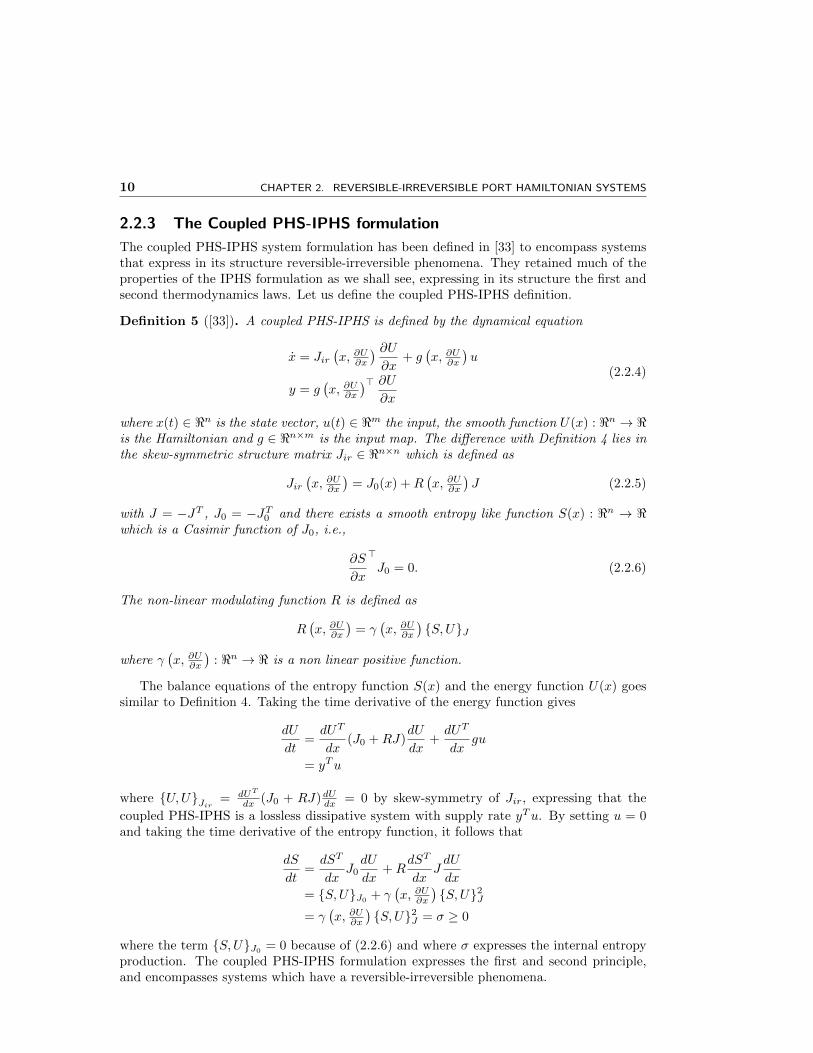
2.2.3 The Coupled PHS-IPHS formulation
The coupled PHS-IPHS system formulation has been defined in [33] to encompass systemsthat express in its structure reversible-irreversible phenomena. They retained much of theproperties of the IPHS formulation as we shall see, expressing in its structure the first andsecond thermodynamics laws. Let us define the coupled PHS-IPHS definition.
Definition 5 ([33]). A coupled PHS-IPHS is defined by the dynamical equation
x = Jir(x, ∂U∂x
) ∂U∂x
+ g(x, ∂U∂x
)u
y = g(x, ∂U∂x
)> ∂U∂x
(2.2.4)
where x(t) ∈ <n is the state vector, u(t) ∈ <m the input, the smooth function U(x) : <n → <is the Hamiltonian and g ∈ <n×m is the input map. The difference with Definition 4 lies inthe skew-symmetric structure matrix Jir ∈ <n×n which is defined as
Jir(x, ∂U∂x
)= J0(x) +R
(x, ∂U∂x
)J (2.2.5)
with J = −JT , J0 = −JT0 and there exists a smooth entropy like function S(x) : <n → <which is a Casimir function of J0, i.e.,
∂S
∂x
>J0 = 0. (2.2.6)
The non-linear modulating function R is defined as
R(x, ∂U∂x
)= γ
(x, ∂U∂x
)S,UJ
where γ(x, ∂U∂x
): <n → < is a non linear positive function.
The balance equations of the entropy function S(x) and the energy function U(x) goessimilar to Definition 4. Taking the time derivative of the energy function gives
dU
dt=dUT
dx(J0 +RJ)
dU
dx+dUT
dxgu
= yTu
where U,UJir = dUT
dx (J0 + RJ)dUdx = 0 by skew-symmetry of Jir, expressing that the
coupled PHS-IPHS is a lossless dissipative system with supply rate yTu. By setting u = 0and taking the time derivative of the entropy function, it follows that
dS
dt=dST
dxJ0dU
dx+R
dST
dxJdU
dx
= S,UJ0 + γ(x, ∂U∂x
)S,U2J
= γ(x, ∂U∂x
)S,U2J = σ ≥ 0
where the term S,UJ0 = 0 because of (2.2.6) and where σ expresses the internal entropyproduction. The coupled PHS-IPHS formulation expresses the first and second principle,and encompasses systems which have a reversible-irreversible phenomena.

2.2. IRREVERSIBLE PORT HAMILTONIAN SYSTEMS - IPHS 11
2.2.4 Casimir functions for Coupled PHS-IPHS
As in port Hamiltonian systems, one can look for Casimir functions for a coupled PHS-IPHS.Let us take C a real function of the states of the systems and suppose that the followingrelation holds
∂C>
∂xJir = 0 (2.2.7)
If we take the time derivative of C, with the condition (2.2.7), it follows that
dC
dt=∂C>
∂x
[Jir
∂U
∂x+ gu
]=∂C>
∂xgu (2.2.8)
If u = 0 then (2.2.8) remains true for every C(x) along the trajectories of the PHS-IPHS,independently of the Hamiltonian U(x).
Definition 6. A Casimir function for a coupled PHS-IPHS (Definition 5) is any functionC(x) : <n → < which satisfies
∂C>
∂xJir = 0 (2.2.9)
Furthermore, as it was shown in (2.2.8), by setting u = 0 then
dC
dt= 0
Thus the Casimir function is a conserved quantity of the system for u = 0, independently
of the Hamiltonian U . If ∂C>
∂x g = 0 then the invariance holds for any input u.
Proposition 2. Let C(x) : <n → < be a Casimir function for the PHS-IPHS in Definition5 if and only if
∂C>
∂xJir = 0 (2.2.10)
where Jir = −J>ir = J0 +RJ is the structure matrix of the PHS-IPHS.
Note that as J0 and J are skew-symmetric, it does not necessarily follow that ∂C>
∂x J0 = 0
and ∂C>
∂x J = 0.The following section studies the example of a non-isothermal RLC system which is a
system than can be interpreted within the framework of the coupled PHS-IPHS.
2.2.5 Example: non-isothermal RLC system
Consider a RLC system connected in series including the dynamics of the thermal effectsof its electrical components. So we can consider that all electrical components, i.e, theresistor r(S); the inductor L(S) and the capacitor C(S) are a function of the temperatureand therefore of the entropy of the system.
The internal energy of the system U(Q,φ, S) shall be the sum of: the energy of thecapacitor; the energy of the inductor and some thermal related energy function Us(S) asso-ciated to the components of the system, with Q being the charge of the capacitor; φ beingthe flux of the inductor and S the entropy of the system.
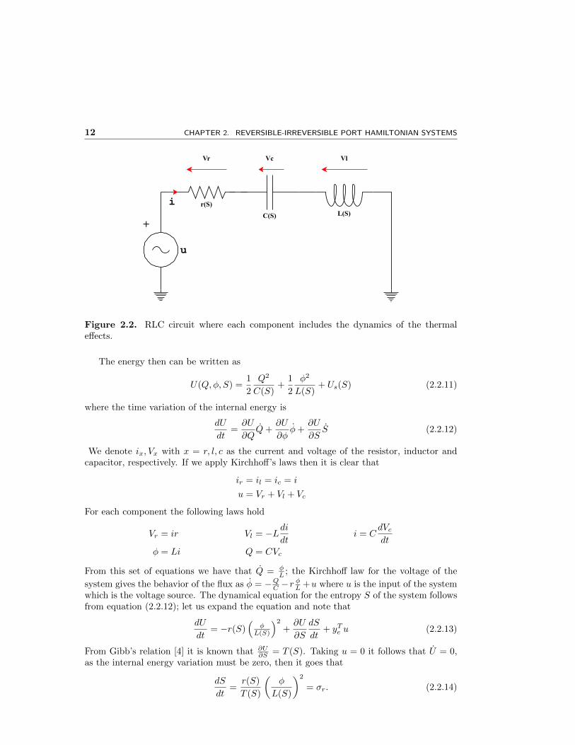
12 CHAPTER 2. REVERSIBLE-IRREVERSIBLE PORT HAMILTONIAN SYSTEMS
r(S)
C(S) L(S)
+
i
Vr Vc Vl
u
Figure 2.2. RLC circuit where each component includes the dynamics of the thermaleffects.
The energy then can be written as
U(Q,φ, S) =1
2
Q2
C(S)+
1
2
φ2
L(S)+ Us(S) (2.2.11)
where the time variation of the internal energy is
dU
dt=∂U
∂QQ+
∂U
∂φφ+
∂U
∂SS (2.2.12)
We denote ix, Vx with x = r, l, c as the current and voltage of the resistor, inductor andcapacitor, respectively. If we apply Kirchhoff’s laws then it is clear that
ir = il = ic = i
u = Vr + Vl + Vc
For each component the following laws hold
Vr = ir Vl = −Ldidt
i = CdVcdt
φ = Li Q = CVc
From this set of equations we have that Q = φL ; the Kirchhoff law for the voltage of the
system gives the behavior of the flux as φ = −QC −rφL +u where u is the input of the system
which is the voltage source. The dynamical equation for the entropy S of the system followsfrom equation (2.2.12); let us expand the equation and note that
dU
dt= −r(S)
(φ
L(S)
)2
+∂U
∂S
dS
dt+ yTe u (2.2.13)
From Gibb’s relation [4] it is known that ∂U∂S = T (S). Taking u = 0 it follows that U = 0,
as the internal energy variation must be zero, then it goes that
dS
dt=r(S)
T (S)
(φ
L(S)
)2
= σr. (2.2.14)

2.2. IRREVERSIBLE PORT HAMILTONIAN SYSTEMS - IPHS 13
The term σr corresponds to the internal entropy production of the system. The PHS-IPHSformulation of the thermodynamic RLC circuit is thenQφ
S
=
0 1 0−1 0 00 0 0
+r
T
φ
L
0 0 00 0 −10 1 0
QCφLT
+
010
u (2.2.15)
where
J0 =
0 1 0−1 0 00 0 0
J =
0 0 00 0 −10 1 0
R =r
T
φ
L
Note that the RLC system (2.2.15) has the structure of the Definition 5 with a structurematrix composed of an irreversible part related to the dissipation and a reversible partrelated to Kirchhoff’s law.
2.2.6 Casimir functions of the non-isothermal RLC system
Now, we shall study if the non-isothermal RLC system (2.2.15) has useful Casimir functions.By proposition 2, we have to look for a function C(x) : <3 → < such that
[∂C∂Q
∂C∂φ
∂C∂S
] 0 1 0
−1 0 − rTφL
0 rTφL 0
= 0
It is easy to note that the system is reduced to
∂C
∂φ= 0
∂C
∂Q= − r
T
φ
L
∂C
∂S
As the first equation imposes that the Casimir has to have no dependency of the flux φ ofthe system, there isn’t a non trivial solution that solves the PDE.
Even though the Casimir functions of a system when we have no input are usually trivial,we shall see in Chapter 3 that they are proven to be a powerful tool in the energy-Casimirapproach when a control input u is considered.
Chapter 3
PASSIVITY BASED CONTROLMETHODS APPLIED TO IPHS
In the present chapter the main contributions of this thesis are shown. The framework ofthe Passivity Based Control (PBC) with emphasis on the control by interconnection plusdamping injection approach (Cbi-Di) is presented.
We first recall the basics of the formulation applied to PHS. In order to do that, somedefinitions about Lyapunov stability and Lasalle’s invariance principle are shown. As anillustrative example, a Cbi-Di controller for the mass-spring-damper system (2.1.8) is ob-tained. Subsequently, we extend the Cbi-Di framework to the control of IPHS; as we shallsee, Casimir functions shall be instrumental in the design. The notion of the availabil-ity function shall complement the control design as it provides candidates for Lyapunovfunctions for the irreversible part of the IPHS.
The example of the CSTR system, whose IPHS model has been obtained in section(2.2.2), is used later to design a controller within the framework of the Cbi-Di controller forPHS-IPHS.
3.1 Passivity Based Control of PHS
The Passivity based control framework has been used to model electrical, mechanical andcomplex physical systems since the control design has a physical interpretation. The PBCframework aims at rendering the closed-loop Hamiltonian function, which has been shownto serve as a candidate for a Lyapunov function, to some desired and useful energy function,which has a new a desired equilibrium dynamic. It provides a systematic framework toachieve stabilization and asymptotic stability for a PHS, and has been used successfully forcontrol design ([25], [27], [37]).
In this section we give the standard definition of the Cbi-Di control for PHS; somedefinitions concerning Lyapunov theorem and the Lasalle’s invariance principle are shownas they are fundamental in the Cbi-Di approach to ensure stability and asymptotic stabilityof the closed-loop system.
3.1.1 Lyapunov Stability Theorem
The Lyapunov stability analysis formalizes the idea that all systems shall tend to a minimumenergy state. It gives a powerful method in stability analysis of non-linear systems and inthe passivity based control framework for PHS it is fundamental, as the energy functionsare candidates for Lyapunov functions.
14
3.1. PASSIVITY BASED CONTROL OF PHS 15
Theorem 1 ([3]). Let D be a compact subset of the state space of a system, containing theequilibrium point x0, and let there be a function V : D → <. The equilibrium point x0 isstable (in the sense of Lyapunov) if V satisfies the following conditions:
1. V (x) ≥ 0, for all x ∈ D
2. V (x) = 0 if and only if x = x0
3. For all x(t) ∈ D,
dV (t)
dt=∂V (t)
∂x
∂x(t)
dt≤ 0
Furthermore, if V (x(t)) is strictly negative, i.e V (x(t)) < 0, then the equilibrium issaid to be asymptotically stable
3.1.2 Lasalle’s Invariance Principle
The Lyapunov stability theorem guarantees asymptotic stability of the system if we canfind a Lyapunov function that is strictly decreasing away from the equilibrium point, as isstated in Theorem 1; but the strictly negative derivative condition on Theorem 1 can berelaxed while ensuring system asymptotic stability. First, we give a definition concerning toan invariant manifold and a positively invariant set. Then we show the Lasalle’s invarianceprinciple.
Definition 7 ([15]). Let Ω ∈ <m ×Rn. The set Ω is said to be an invariant manifold if
(x(0), ξ(0)) ∈ Ω⇔ (x(t), ξ(t)) ∈ Ω,∀t ≥ 0 (3.1.1)
Given t = t0. A set Ω is set to be positively invariant if x(t0) ∈ Ω, then x(t) ∈ Ω for allt ≥ t0.
For example, the multi level set Ωκ = (x, ξ) ∈ <n ×<m | ξ = F (x) + κ is an invariantmanifold, where κ is a vector of constants. Next, we define the Lasalle’s invariance principle.
Theorem 2 ([15]). Consider the non-linear dynamical system x(t) = f(x(t)) with x(0) =x0. Assume that Dc ⊂ D is a compact positively invariant set with respect to the non-linearsystem, and assume there exits a continuously differentiable function V : Dc → < such
that V (x)f(x) ≤ 0, x ∈ Dc. Let Ω.=x ∈ Dc : V (x)f(x) = 0
and let M be the largest
invariant set contained in Ω. If x(0) ∈ Dc, then x(t)→M as t→∞.
3.1.3 Control by Interconnection of PHS
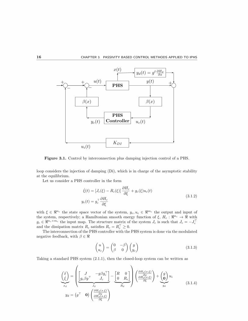
The paradigm of control by interconnection has been used within the framework of passivitybased control techniques for stabilization. Control by interconnection aims at shaping theHamiltonian function and the structure matrices by state feedback with a controller, whichis also a PHS system; the closed-loop system has proven to be also a PHS. The next stepis to find useful Casimir functions for this new PHS, as they allow to move the equilibriumpoint of the Hamiltonian energy function; this is done by solving a set of PDE [37].
We shall follow figure 3.1 for the control design; the first loop considers the control byinterconnection (Cbi) part, which is in charge of the stability of the system, while the second
16 CHAPTER 3. PASSIVITY BASED CONTROL METHODS APPLIED TO IPHS
β(x)
PHS
PHSController
KDI
x(t)
u(t) y(t)
yd(t) = gt ∂Hd
∂x
+
ui(t)
−
β(x)
uc(t)yc(t)
−++
1
Figure 3.1. Control by interconnection plus damping injection control of a PHS.
loop considers the injection of damping (Di), which is in charge of the asymptotic stabilityat the equilibrium.
Let us consider a PHS controller in the form
ξ(t) = [Jc(ξ)−Rc(ξ)]∂Hc
∂ξ+ gc(ξ)uc(t)
yc(t) = g>c∂Hc
∂ξ
(3.1.2)
with ξ ∈ <nc the state space vector of the system, yc, uc ∈ <mc the output and input ofthe system, respectively; a Hamiltonian smooth energy function of ξ, Hc : <nc → < withgc ∈ <nc×mc the input map. The structure matrix of the system Jc is such that Jc = −J>cand the dissipation matrix Rc satisfies Rc = R>c ≥ 0.
The interconnection of the PHS controller with the PHS system is done via the modulatednegative feedback, with β ∈ < (
uuc
)=
(0 −ββ 0
)(yyc
)(3.1.3)
Taking a standard PHS system (2.1.1), then the closed-loop system can be written as
(x
ξ
)︸︷︷︸xd
=
[
J −gβg>cgcβg
> Jc
]︸ ︷︷ ︸
Jd
−[R 00 Rc
]︸ ︷︷ ︸
Rd
(∂Hd(x,ξ)
∂x∂Hd(x,ξ)
∂ξ
)+
(g0
)︸︷︷︸gd
ui
yd =(g> 0
)(∂Hd(x,ξ)∂x
∂Hd(x,ξ)∂ξ
) (3.1.4)

3.1. PASSIVITY BASED CONTROL OF PHS 17
which is a PHS system with structure matrix Jd = −J>d , dissipation matrix Rd = R>d ≥ 0,both matrices of order (n+nc)×(n+nc) and the input map gd with order (n+nc)×(m+mc),where 0 is a null matrix of order nc ×mc; the closed-loop Hamiltonian energy function isHd = H +Hc.
The next step is to find structural invariant functions. The Casimir functions can berestricted, without loss of generality, to the set of functions [37]
Ci(x, ξi) = Fi(x)− ξi, i = 1, .., l ≤ nc (3.1.5)
where Ci is the Casimir function associated to the state ξi of the controller and F (x) =[F1, ..., Fl] ∈ <l is a collection of smooth functions Fi of x. If the Casimir function exists,the relation ξ−F (x) = κ with κ = [κ1, ..., κl] ∈ <l a vector of constants that depend on theinitial states of the plant and the controller, holds on every invariant set Ω = (x, ξ) ∈ <x×ξ |C(x, ξ) = −κ. The closed-loop Hamiltonian energy candidate to a Lyapunov function, canbe rewritten as a function of the states of the PHS system as Hd(x) = H(x)+Hc(F (x)+κ),and the shaping control input as the negative feedback
ue = −yc (F (x) + κ) = −g>c∂Hc
∂ξ(3.1.6)
The Casimir functions are invariants of the structure of the closed-loop system (3.1.4), which
means that the relation ∂C>
∂xdJd = 0 is satisfied. This condition leads to the set of partial
differential equations known as matching equations
∂F>
∂xJ∂F
∂x= Jc
R∂F
∂x= 0
Rc = 0
∂F>
∂xJ = gcβg
>
(3.1.7)
The third equation in (3.1.7) is known as the dissipation obstacle ([37], [38]) since it dictatesthat the variables of the system that has dissipation cannot be shaped. Assuming that suchF smooth function exists then the control action (3.1.6) shapes the Hamiltonian energy ofthe system, and the function Hd(x) = H(x)+Hc(F (x)+κ) is a Lyapunov function candidatefor the closed-loop system and the system
x = [J −R]∂Hd
∂x+ gui
yd = g>∂Hd
∂x
is stable with respect to some desire equilibrium point x∗ for a particular choice of ξ∗.
3.1.4 Damping injection
The energy shaping control action renders the Hamiltonian energy function into a Lyapunovfunction candidate for the system with a strict minimum in some desired equilibrium pointx∗ for a particular choice of ξ∗. The damping injection control action renders the system
18 CHAPTER 3. PASSIVITY BASED CONTROL METHODS APPLIED TO IPHS
asymptotically stable. Taking x∗ as the minimum of the Hamiltonian function, and settingthe control input
ui = −Kyd = −Kg> ∂Hd
∂x(3.1.8)
where K = KT ≥ 0 is a symmetric semi positive matrix, guarantees asymptotic stabilityfor the closed-loop system at the point (x∗, ξ∗) by the application of Lasalle’s invarianceprinciple. In fact, with the control action (3.1.8) and setting M = gKgT ≥ 0 the closed-loop system can be written as
x(t) = (J −M)∂Hd
∂x
Taking the time derivative of the closed-loop system we obtain
dHd
dt=∂H>d∂x
(J −M)∂Hd
∂x= Hd, HdJ − Hd, HdM= −Hd, HdM < 0
Since Hd is a Casimir function of J it follows that Hd, HdJ = 0. By Lasalle’s invarianceprinciple (Theorem 2, section 3.1.2) then the closed-loop system converges asymptoticallyto x∗.
3.1.5 Example: Cbi-Di for the MSD system
In this section we design, as an example of the framework, a Cbi-Di controller for the MSDsystem analyzed in section 2.1.3. Since the system has dissipation in the p coordinate, weaim at rendering the closed-loop system to a point x∗ = (q∗, 0). Consider the PHS controller
ξ = (Jc −Rc)∂Hc
∂ξ+ gcuc
We look for a Casimir function of the form C(q, p) = F − ξ such that ξ = F + κ, withF ∈ < a smooth function of the states of the system and κ ∈ < a constant that depends onthe initial states of the controller and the system. For simplicity, we take β(x) = 1. Thegradient F with respect to the states of the system takes the form
∂F>
∂x=(∂F∂q
∂F∂p
)The first, second and fourth equation of (3.1.7) give, respectively
Jc = 0,∂F
∂p= 0,
∂F
∂x= gc
where ∂F∂p was expected to be null due to the dissipation obstacle on the coordinate of
the state. By taking gc = 1 for simplicity, and by simple integration F (q, p) = F (q) = q,where it is easy to note that ξ = q. We choose the following Hamiltonian as a candidateLyapunov energy function
Hd = (k + k0)(q − q∗)2
2+
p2
2M
3.2. PASSIVITY BASED CONTROL OF IPHS 19
where the energy of the controller is such that Hc = Hd − H, where we recall that H =
k q2
2 + p2
2M . The controller energy function is then chosen as
Hc = k0q2
2− (k + k0)qq∗ +
(k + k0)
2(q∗)2 = k0
ξ2
2− (k + k0)ξq∗ +
(k + k0)
2(q∗)2
The PHS controller can then be expressed as
ξ = uc
yc = k0ξ − (k + k0)q∗(3.1.9)
which is a controller with integral-proportional action. The energy shaping control actionis given by
ue = −g>c∂Hc
∂ξ= (k + k0)q∗ − k0ξ
For the damping injection control action, take K ∈ < such that M = gKg> ∈ <2×2 ≥ 0. Apossible choice for K is to take K = α ≥ 0 a tuning parameter which gives
M =
[0 00 α
]with M being a semi positive matrix. The damping injection control action can be obtainedas
ui = −Kg> ∂Hd
∂x= −α
[0 1
] [(k + k0)(q − q∗)pm
]= −α p
m
The closed-loop system, with the addition of damping, can be written as[qp
]=
([0 1−1 0
]−[0 00 α
])[(k + k0)(q − q∗)
pM
]
3.2 Passivity Based Control of IPHS
In this section the main contributions of this thesis are shown with the synthesis of a controlby interconnection plus damping injection (Cbi-Di) controller framework for the control ofIPHS. As IPHS retain much of the PHS, PBC techniques such as Cbi-Di can be furtherexplored to the control of IPHS. Thus we synthesize a Cbi-Di controller through a systematicdesign. We shall exploit Definition 5 which encompass systems with reversible-irreversiblephenomena. This definition shows that an IPHS system can be seen as a compositionof a conservative part and an irreversible part. Furthermore, we shall exploit Definition 8which is the availability function of an irreversible process and serves as candidate Lyapunovfunction.
The control by interconnection plus damping injection is done following Figure 3.2. TheIPHS system is interconnected with an IPHS controller in the first loop through a statespace modulated function, and is in charge of placing the closed-loop equilibrium point.The controller is used to render the closed-loop Hamiltonian energy function such that ithas a minimum at the desire equilibrium point and is now a candidate Lyapunov functionby the use of Definition 8. A second loop, with a damping injection control action is design

20 CHAPTER 3. PASSIVITY BASED CONTROL METHODS APPLIED TO IPHS
to ensure asymptotic stability of the closed-loop system. The damping injection controlinput is performed with respect to the closed-loop system output which is the conjugatedoutput to the closed-loop Hamiltonian function.
The final control input takes the form u = ue + ui where ue is the input due to theenergy shaping action and ui is the input due to the damping injection action.
3.2.1 Control by interconnection of IPHS
β(x)
IPHS
IPHSController
KDI
x(t)
u(t) y(t)
yd(t) = gt ∂Ud
∂x
+
ui(t)
−
β(x)
uc(t)yc(t)
−++
1
Figure 3.2. Control by interconnection plus damping injection control of an IPHS.
Let us consider the IPHS controller
ξ = R(ξ, ∂Uc
∂ξ
)Jc∂Uc∂ξ
(ξ) + gc
(ξ, ∂Uc
∂ξ
)uc(t)
yc = gTc
(ξ, ∂Uc
∂ξ
) ∂Uc∂ξ
(ξ)
(3.2.1)
with ξ ∈ <nc the state space vector yc, uc ∈ <mc the output and input of the system,respectively. The mapping gc(ξ) ∈ <nc×mc , a Hamiltonian smooth function Uc(ξ) and
R(ξ, ∂Uc
∂ξ
)a modulating non-linear function. The interconnection between the states is via
the modulated power-preserving interconnection(ueuc
)=
(0 −β(x)
β(x) 0
)(yyc
)(3.2.2)
where β(x) ∈ <. The closed-loop system, following the first loop of figure 3.2, between astandard IPHS (2.2.4) and the IPHS controller (3.2.1) takes the form(
x
ξ
)=
(Jir −gβgTc
gcβgT RJc
)︸ ︷︷ ︸
Jd
(∂Ud(x,ξ)
∂x∂Ud(x,ξ)
∂ξ
)+
(g0
)ui (3.2.3)
3.2. PASSIVITY BASED CONTROL OF IPHS 21
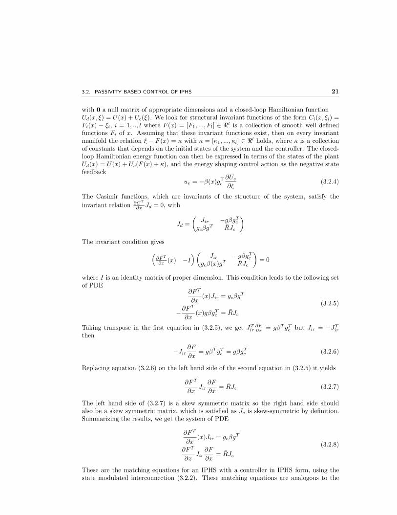
with 0 a null matrix of appropriate dimensions and a closed-loop Hamiltonian functionUd(x, ξ) = U(x) + Uc(ξ). We look for structural invariant functions of the form Ci(x, ξi) =Fi(x) − ξi, i = 1, .., l where F (x) = [F1, ..., Fl] ∈ <l is a collection of smooth well definedfunctions Fi of x. Assuming that these invariant functions exist, then on every invariantmanifold the relation ξ − F (x) = κ with κ = [κ1, ..., κl] ∈ <l holds, where κ is a collectionof constants that depends on the initial states of the system and the controller. The closed-loop Hamiltonian energy function can then be expressed in terms of the states of the plantUd(x) = U(x) + Uc(F (x) + κ), and the energy shaping control action as the negative statefeedback
ue = −β(x)g>c∂Uc∂ξ
(3.2.4)
The Casimir functions, which are invariants of the structure of the system, satisfy the
invariant relation ∂C>
∂x Jd = 0, with
Jd =
(Jir −gβgTc
gcβgT RJc
)The invariant condition gives(
∂FT
∂x (x) −I)( Jir −gβgTc
gcβ(x)gT RJc
)= 0
where I is an identity matrix of proper dimension. This condition leads to the following setof PDE
∂FT
∂x(x)Jir = gcβg
T
−∂FT
∂x(x)gβgTc = RJc
(3.2.5)
Taking transpose in the first equation in (3.2.5), we get JTir∂F∂x = gβT gTc but Jir = −JTir
then
−Jir∂F
∂x= gβT gTc = gβgTc (3.2.6)
Replacing equation (3.2.6) on the left hand side of the second equation in (3.2.5) it yields
∂FT
∂xJir
∂F
∂x= RJc (3.2.7)
The left hand side of (3.2.7) is a skew symmetric matrix so the right hand side shouldalso be a skew symmetric matrix, which is satisfied as Jc is skew-symmetric by definition.Summarizing the results, we get the system of PDE
∂FT
∂x(x)Jir = gcβg
T
∂FT
∂xJir
∂F
∂x= RJc
(3.2.8)
These are the matching equations for an IPHS with a controller in IPHS form, using thestate modulated interconnection (3.2.2). These matching equations are analogous to the
22 CHAPTER 3. PASSIVITY BASED CONTROL METHODS APPLIED TO IPHS
case of control by interconnection of PHS with the difference that Jir depends on the mod-ulating functions R and that the control structure Jc includes a modulating function R.Assuming that the smooth function F (x) exists, the control law (3.2.4) shapes the closed-loop Hamiltonian function as Ud(x) = U(x) +Uc(F (x+κ)). Furthermore, the energy-inputallows to interpret the closed-loop system as an IPHS. In effect, notice that
dx
dt= RJir
∂U
∂x− g βgc
∂(Uc F )
∂ξ︸ ︷︷ ︸ue
(3.2.9)
Using the first equation in (3.2.8) and the skew-symmetric property of Jir, the relation(3.2.9) can be rewritten as
dx
dt= RJir
∂U
∂x+ Jir
∂F
∂x
∂(Uc F )
∂ξ
= RJir∂U
∂x+ Jir
∂Uc∂x
Finally, by simple factorization and adding an input ui to the closed-loop system, we get
x = Jir∂Ud∂x
+ gui
yd = g>∂Ud∂x
(3.2.10)
where yd is the passive output defined with respect to Ud(x). This approach allows tosee the closed-loop system as an IPHS; i.e, without destroying the structure of IPHS, andtherefore it can be interconnected with others IPHS and interpreted within the frameworkof the energy-Casimir plus damping design for control purposes. Next, we calculate the timederivative of the entropy of the closed-loop system
dS
dt=∂S>
∂xJ0∂Ucl∂x
+R∂S>
∂xJ∂Ucl∂x
= R∂S>
∂xJ∂U
∂x︸ ︷︷ ︸σ(t)
+R∂S>
∂xJ∂Uc∂x︸ ︷︷ ︸
σc(t)
where σ ≥ 0 is the internal entropy variation of the system and σc is the external entropyvariation due to the inputs of the system. As the control objective is to set a desired entropy,σc = −σ in steady state.
The time variation of the closed-loop energy function is now given by
dUddt
= y>d ui (3.2.11)
Since the internal energy function of irreversible thermodynamic systems does not have astrict minimum, it does not qualify as a candidate Lyapunov function. A standard candi-date Lyapunov function for control purposes is the availability function ([1], [39], [19]). Theavailability function (figure 3.3) uses the convexity of the internal energy with the assump-tion that one of the extensive variables is fixed, to construct a strictly convex extension

3.2. PASSIVITY BASED CONTROL OF IPHS 23
Figure 3.3. The red plot shows the internal energy of an irreversible process and the blackline is the supporting hyper plane at a point x∗. The availability function is the differencebetween the two.
which serves as Lyapunov function for a desired dynamical equilibrium. This approach hasbeen widely used in the control of thermodynamic systems in the last decade ([16], [17],[31]). We shall use the availability function as the target Lyapunov candidate function ofthe closed-loop system for the irreversible part of the IPHS in the energy-shaping design.The availability function is then defined as follows.
Definition 8 ([31]). The energy based availability function is x defined as
A(x, x∗) = U(x)− U(x∗)− ∂U
∂x(x∗)T (x− x∗) (3.2.12)
with U(x) being the internal thermodynamic energy of the system and x∗ the desired equi-librium point of a thermodynamic variable x.
3.2.2 Damping Injection
The energy shaping input shapes the energy of the system into a new equilibrium dynamicsand guarantees the closed-loop stability of the system in the sense of Lyapunov, but onehave yet to guarantee the asymptotic stability at the equilibrium point.
Let’s suppose that the closed-loop IPHS (3.2.10) has a minimum at x∗ and set a damping
24 CHAPTER 3. PASSIVITY BASED CONTROL METHODS APPLIED TO IPHS
injection input as
ui = −Kyd = −Kg> ∂Ud∂x
(3.2.13)
with K = K> > 0. We shall show that this control action renders the system dissipative,i.e, adds a positive definite matrix M to the structure matrix Jir of the system. In fact, bysetting ui as the damping input in the closed-loop system (3.2.10) we get
x(t) = (Jir − gKgT )∂Ud∂x
(3.2.14)
The time derivative of the closed-loop energy function is then given by
dUddt
=dUTddx
(Jir − gKgT )∂Ud∂x
= Ud, UdJir − Ud, UdM= −Ud, UdM < 0
since Ud, UdJir = 0 and whereM = gKgT ≥ 0. By Lasalle’s invariance principle (Theorem2) the closed-loop system converges asymptotically to x∗, ξ∗ in the largest positively invariantset Ω = (x, ξ) ∈ <x×ξ | C(x, ξ) = −κ.
Next, we give a proposition that encompasses the control by interconnection plus damp-ing injection for IPHS.
Proposition 3. Let Σ be an IPHS system of order n given by Definition 5 and Σc bean IPHS controller of order nc given in (3.2.1). Consider the interconnection between Σand Σc via the state modulated relation in (3.2.2). Without loss of generality, considerthe positively invariant manifold Ω = (x, ξ) ∈ <x×ξ | C(x, ξ) = −κ such that for everyrelation ξi − Fi(x) = κi, i = 1, ..., l ≤ nc ≤ n it satisfies the PDE (3.2.8) and whereF = [F1, ..., Fl] ∈ <l, κ = [κ1, ..., κl] ∈ <l are a collection of smooth functions of the statespace x, and a collection of constants that depend on the initial states of the system and thecontroller, respectively. The collection C(x, ξ) are Casimirs of the closed-loop system if thecollection of smooth functions F satisfy the PDE
∂FT
∂x(x)Jir = gcβg
T
∂FT
∂xJir
∂F
∂x= RJc
If there exists a function Uc(ξ) such that the closed-loop Hamiltonian energy function Ud(x)is a candidate for a Lyapunov function and has a strict minimum at the point (x∗) for aparticular election of ξ∗, then (x∗, ξ∗) is a stable equilibrium point for the closed-loop system.Furthermore, the control action
ui = −Kyd = −Kg> ∂Ud∂x
for a certain K = K> ≥ 0 such that M = gKg> ≥ 0 renders the system asymptoticallystable.
Proof. The proof has been shown in subsections (3.2.1) and (3.2.2)

3.2. PASSIVITY BASED CONTROL OF IPHS 25
3.2.3 Cbi-Di control of the CSTR system
In this section a Cbi-Di controller for the CSTR system is obtained. Proposition 3 shall beused in order to design the controller.
The CSTR system has states x =[n1 n2 · · · nm S
]>. We shall parametrize the
design and look for Casimir functions of the form C1(n1, ξ1) = F1(n1)−ξ1,· · · , Cm(nm, ξm) =Fm(nm) − ξm and Cm+1(S, ξm+1) = Fm+1(S) − ξm+1 such that ξi = Fi(ni) + κi withi = 1, ...,m and ξm+1 = Fm+1(S) + κm+1.
We take a purely irreversible IPHS controller (2.2.1) as the CSTR is also purely irre-versible; the controller then takes the form
ξ = RcJc∂Uc∂ξ
+ gcuc
yc = g>c∂Uc∂ξ
(3.2.15)
where ξ =[ξ1 · · · ξm+1
]> ∈ <m+1, Jc ∈ <m+1×m+1, β ∈ < a scalar function and theinput map
gc =
g11 g12
......
g(m+1)1 g(m+1)2
where each term gij = gij(ξ) can be dependent on the states of the system.
Since the CSTR is purely irreversible, we set as desired Hamiltonian energy function forthe closed-loop system, the energy based availability function
A(t) = Ud = U(x)− [U(x∗) +∂UT
∂x(x∗)(x− x∗)] (3.2.16)
where x∗ is the new equilibrium point. A simple choice for the energy of the controller is totake Uc = Ud − U , hence
Uc = −[U(x∗) +∂UT
∂x(x∗)(x− x∗)]
=
m∑i=1
(−µ∗ini + µ∗in∗i ) + (−T ∗S + T ∗S∗)− U(n∗1, · · · , n∗m, S∗)
The parametrization of the Casimir function and the election of the Controller leads to thefollowing condition on F
∂F
∂x=
−µ∗1 0 · · · 0
0. . . · · · 0
... · · · −µ∗m...
0 0 · · · −T ∗
where by integration we have F (ni) = −niµ∗i , i = 1, ...,m and F (S) = −T ∗S. Notice thatthe CSTR system is purely irreversible with structure matrix Jir = RJ and J0 = 0. By
26 CHAPTER 3. PASSIVITY BASED CONTROL METHODS APPLIED TO IPHS
applying the first of the matching equations (3.2.8) it follows
∂F>
∂xJir = R
0 · · · 0 −µ∗1ν1
0 · · · 0...
.... . .
... −µ∗mνmT ∗ν1 · · · T ∗νm 0
And the right side of the first equation is
βgcg> = β
g11n1 · · · g11nm g11φ+ g12
Tg21n1 · · · g21nm g21φ+ g22
T...
. . ....
...g(m+1)1n1 · · · g(m+1)1nm g(m+1)1φ+
g(m+1)2
T
By equality, gi1 = 0 and gi2 = −Tµ∗i νi,∀i = 1, ...,m with
β = R g(m+1)2 = −Tg(m+1)1φ g(m+1)1 = T ∗νini
The equality g(m+1)1ni
νi= T ∗ has to be true ∀i = 1, ...,m. The system has a solution if the
relationn1
ν1= · · · = nm
νm(3.2.17)
holds for every i = 1, ...,m. In [30], for batch reactors the equality (3.2.17) is the expressionof De Donder’s extent of reaction
n0i − niνi
= δ
where this property can be extended to the CSTR under Assumption 1. This condition hasbeen obtained in [31] where an IDA-PBC like approach is used to design a controller for aclass of CSTR. Then the input map gc of the controller, can be written as
gc =
0 −Tµ∗1ν1
......
0 −Tµ∗mνmT ∗/δ TT ∗φ(ξ)/δ
(3.2.18)
The structure matrix Jc and the modulating function Rc of the controller are defined bythe third equation in (3.2.8)
∂FT
∂xJir
∂F
∂x=rV
TT ∗
0 · · · 0 µ∗1ν1
.... . .
......
0 µ∗mνm−µ∗1ν1 · · · −µ∗mνm 0
As the right hand side of the third matching equation (3.2.8) is RcJc, then it follows that
Jc =
0 · · · 0 µ∗1ν1
.... . .
......
0 µ∗mνm−µ∗1ν1 · · · −µ∗mνm 0
Rc =rV
TT ∗ (3.2.19)
3.2. PASSIVITY BASED CONTROL OF IPHS 27
Note that by the parametrization of the Casimir functions, i.e, ξi = Fi(ni) +κi, i = 1, ...,mand ξm+1 = Fm+1(S) + κm+1, then the controller energy can be written as
Uc(ξ) =
m∑i=1
(Fi(ni) + κi) + (Fm+1(S) + κm+1)− U(n∗1, ..., n∗m, S
∗) (3.2.20)
Hence,∂UT
c
∂ξ =[1 · · · 1
]. The IPHS controller then takes the form
ξ1...
ξm+1
=rV
TT ∗
0 · · · 0 µ∗1ν1
.... . .
......
0 µ∗mνm−µ∗1ν1 · · · −µ∗mνm 0
1...11
+
0 −Tµ∗1ν1
......
0 −Tµ∗mνmT ∗/δ TT ∗φ(ξ)/δ
uc
yc = gTc
1...1
The energy shaping control action is then given by ue = −βgTc ∂Uc
∂ξ , which results
ue = −rVT
[T/δ
−T∑mi=1 µ
∗i νi − TT ∗φ(x)/δ
](3.2.21)
The closed-loop system then can be expressed as
x(t) =rV
T
0 · · · 0 ν1
0 · · · 0...
0 · · · 0 νm−ν1 · · · −νm 0
µ1 − µ∗1
...µm − µ∗mT − T ∗
+
[n 0
φ(x) 1/T
]ui
By proposition 3, a damping injection input is needed to guarantee asymptotic stability.We design K ∈ <2×2 such that M = gKg> ≥ 0. An easy choice is to take
K = α
[0 00 T 2
]for some tuning parameter α ≥ 0 which gives
M =
0 · · · · · · 0...
. . ....
.... . .
...0 · · · · · · α
∈ <m+1×m+1
The gradient of the Hamiltonian energy function Ud is
∂Ud∂x
=[µ1 − µ∗1 · · · µm − µ∗m T − T ∗
]>and then the damping injection input, which we recall can be computed as ui = −KgT ∂Ud
∂x ,takes the form
ui = −α[
0T (T − T ∗)
](3.2.22)

28 CHAPTER 3. PASSIVITY BASED CONTROL METHODS APPLIED TO IPHS
The closed-loop system becomes
x = (−gKgT +RJ)∂Ud∂x
=
rVT
0 · · · 0 ν1
0 · · · 0...
0 · · · 0 νm−ν1 · · · −νm 0
−
0 · · · · · · 0...
. . ....
.... . .
...0 · · · · · · α
µ1 − µ∗1
...µm − µ∗mT − T ∗
Let us verify the time derivative of the closed-loop Hamiltonian function.
dUddt
= −∂U>d
∂xM∂Ud∂x
= −α(T − T ∗)2 ≤ 0
where the asymptotic stability follows by Lasalle’s invariance principle in a sufficient smallregion of T = T ∗ under Assumption 1, which states that there is only one equilibriumfor each temperature, and then V = 0 only at T = T ∗. We point out that the controllersynthesized with the Cbi-Di framework for IPHS is equivalent to the one in [31] where anIDA-PBC like approach was used.
Chapter 4
A CASE STUDY: THEGAS-PISTON SYSTEM
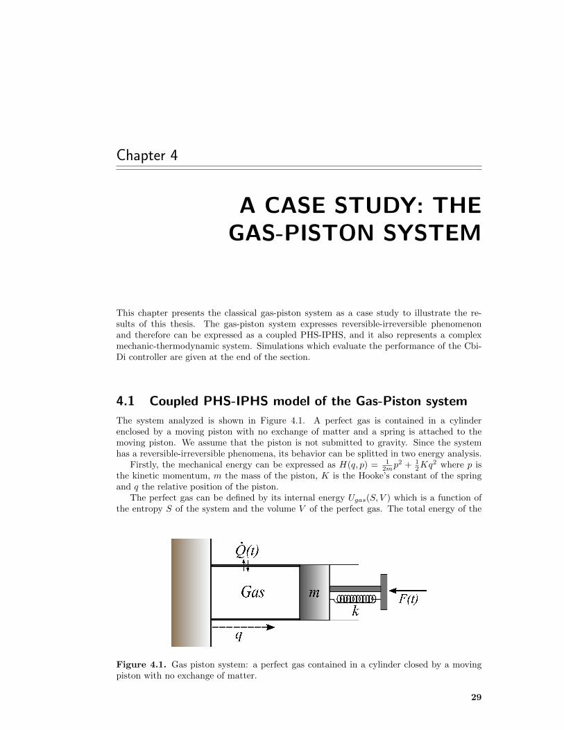
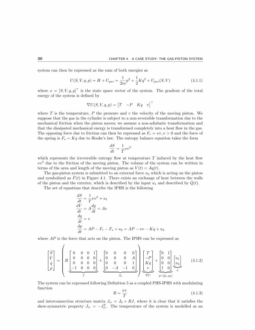
This chapter presents the classical gas-piston system as a case study to illustrate the re-sults of this thesis. The gas-piston system expresses reversible-irreversible phenomenonand therefore can be expressed as a coupled PHS-IPHS, and it also represents a complexmechanic-thermodynamic system. Simulations which evaluate the performance of the Cbi-Di controller are given at the end of the section.
4.1 Coupled PHS-IPHS model of the Gas-Piston system
The system analyzed is shown in Figure 4.1. A perfect gas is contained in a cylinderenclosed by a moving piston with no exchange of matter and a spring is attached to themoving piston. We assume that the piston is not submitted to gravity. Since the systemhas a reversible-irreversible phenomena, its behavior can be splitted in two energy analysis.
Firstly, the mechanical energy can be expressed as H(q, p) = 12mp
2 + 12Kq
2 where p isthe kinetic momentum, m the mass of the piston, K is the Hooke’s constant of the springand q the relative position of the piston.
The perfect gas can be defined by its internal energy Ugas(S, V ) which is a function ofthe entropy S of the system and the volume V of the perfect gas. The total energy of the
Figure 4.1. Gas piston system: a perfect gas contained in a cylinder closed by a movingpiston with no exchange of matter.
29
30 CHAPTER 4. A CASE STUDY: THE GAS-PISTON SYSTEM
system can then be expressed as the sum of both energies as
U(S, V, q, p) = H + Ugas =1
2mp2 +
1
2Kq2 + Ugas(S, V ) (4.1.1)
where x = [S, V, q, p]> is the state space vector of the system. The gradient of the totalenergy of the system is defined by
∇U(S, V, q, p) =[T −P Kq v
]>where T is the temperature, P the pressure and v the velocity of the moving piston. Wesuppose that the gas in the cylinder is subject to a non-reversible transformation due to themechanical friction when the piston moves; we assume a non-adiabatic transformation andthat the dissipated mechanical energy is transformed completely into a heat flow in the gas.The opposing force due to friction can then be expressed as Fr = νv, ν > 0 and the force ofthe spring is Fs = Kq due to Hooke’s law. The entropy balance equation takes the form
dS
dt=
1
Tνv2
which represents the irreversible entropy flow at temperature T induced by the heat flowνv2 due to the friction of the moving piston. The volume of the system can be written interms of the area and length of the moving piston as V (t) = Aq(t).
The gas-piston system is submitted to an external force u2 which is acting on the pistonand symbolized as F (t) in Figure 4.1. There exists an exchange of heat between the wallsof the piston and the exterior, which is described by the input u1 and described by Q(t).
The set of equations that describe the IPHS is the following
dS
dt=
1
Tνv2 + u1
dV
dt= A
dq
dt= Av
dq
dt= v
dp
dt= AP − Fr − Fs + u2 = AP − νv −Kq + u2
where AP is the force that acts on the piston. The IPHS can be expressed as
S
Vqp
=
R
0 0 0 10 0 0 00 0 0 0−1 0 0 0
︸ ︷︷ ︸
J
+
0 0 0 00 0 0 A0 0 0 10 −A −1 0
︸ ︷︷ ︸
J0
T−PKqv
︸ ︷︷ ︸∇U
+
0 10 00 01 0
︸ ︷︷ ︸g=[g1,g2]
[u1
u2
]︸︷︷ ︸u
(4.1.2)
The system can be expressed following Definition 5 as a coupled PHS-IPHS with modulatingfunction
R =νv
T(4.1.3)
and interconnection structure matrix Jir = J0 + RJ , where it is clear that it satisfies theskew-symmetric property Jir = −JTir. The temperature of the system is modelled as an
4.1. COUPLED PHS-IPHS MODEL OF THE GAS-PISTON SYSTEM 31
exponential function of the entropy T (S) = T0eS/c ([7]) where T0 and c are constants that
depend on the system. Finally, the temperature, the volume and the pressure of the gasinside the piston can be related with the law of the ideal gases as PV = rTN , where N isthe number of moles and r the ideal gas constant.
4.1.1 Cbi-Di control of the Gas-Piston system
In this section, we apply Proposition 3 to synthesize a Cbi-Di controller for the gas-pistonsystem. This system expresses irreversible phenomena in the entropy S and volume V ofthe system; the momentum p and the position q express the reversible part of the system.Note that the position and the volume are correlated by V (t) = Aq(t). Then, if a certainequilibrium q∗ is imposed, then a certain equilibrium V ∗ = Aq∗ is obtained.
The design shall be divided in two parts: in a first approach, we design a controller whichstabilizes the system at the point (S, V, q, p) = (S, V ∗, q∗, 0) by using the input u2, which isthe force acting on the piston; in a second approach, a controller is designed to control thepurely irreversible process S of the system, by using the input u1 which is the exchange ofheat.
Step 1: Control of q,p and V
We look for Casimir functions for the system (4.1.2) of the form C(x, ξ) = F (x) − ξ suchthat ξ − F (x) = κ. The aim is to render the mechanical part of the system, which relatesthe position q and the momentum p of the system with the input u2. We take then as ourinput map
g1 = [0 0 0 1]>
The IPHS controller is defined then by xc = ξ ∈ <, Jc ∈ <, β ∈ < a scalar, and the inputmap gc ∈ <, where we take for simplicity gc = 1. The controller then takes the form
ξ = RcJc∂Uc∂ξ
+ uc (4.1.4)
where Uc is the energy of the controller. By applying the matching equations (3.2.8), thefirst one gives
∂F>
∂xJir =
[−R∂F
∂p −A∂F∂p −∂F∂p R∂F
∂S +A ∂F∂V + ∂F
∂q
]gcβg
>1 =
[0 0 0 β
]From the equality it follows that
∂F
∂p= 0, R
∂F
∂S+A
∂F
∂V+∂F
∂q= β
The election and solution of the PDE is motivated by the election of a proper energyfunction for the system. Since the system has a reversible-irreversible phenomenon, we usethe framework of the availability function for the irreversible part. Further, the aim is torender the closed-loop Hamiltonian function as
Ud1(S, V, q, p) = A1(S, V ) +1
2mp2 +
1
2(K +K0)(q − q∗)2
32 CHAPTER 4. A CASE STUDY: THE GAS-PISTON SYSTEM
where A1(S, V ) = Ugas(S, V ) − [Ugas(S∗, V ∗) − P ∗(V − V ∗)] is the availability function
(8) for the irreversible coordinate, associated to the volume of the system. We recall from(4.1.1) that the internal energy of the system is
U(S, V, q, p) = H + Ugas =1
2mp2 +
1
2Kq2 + Ugas(S, V )
Since the energy of the closed-loop system can also be expressed as Ud1 = H + Ugas + Uc,then the simplest choice for the election of Uc is given by
Uc = Ud1 − U
= P ∗(V − V ∗)− Ugas(S∗, V ∗) +1
2K0q
2 − (K +K0)qq∗ +1
2(K +K0)(q∗)2
The controller energy suggests that the following elections
∂F
∂p= 0,
∂F
∂S= 0,
∂F
∂V= α1,
∂F
∂q= α2 + α3q
which gives F = α1V + α2q + α3
2 q2, allow to express the energy of the controller as Uc =
F + κ = ξ with α1 = −P ∗, α2 = −(K +K0)q∗, α3 = K0 and κ = −P ∗V ∗ −Ugas(S∗, V ∗) +12 (K +K0)q2
0 , which results in ∂Uc
∂ξ = 1.
The third equation of (3.2.8) gives the condition on the structure matrix Jc of thecontroller, which results in Jc = 0 and β = AP ∗ − (K +K0)q∗ +K0q. The IPHS controllercan then be written as the simple integrator
ξ = uc
The energy shaping control action is given by
ue1 = −βg>c∂Uc∂ξ
= −AP ∗ + (K +K0)q∗ −K0q (4.1.5)
By Proposition 3, for the damping injection, we take K1 ∈ < such that M1 = g1K1g>1 ∈
<4×4 ≥ 0. An easy choice is to take K1 = α1 ≥ 0 with α1 a tuning parameter, which gives
M1 =
0 0 0 00 0 0 00 0 0 00 0 0 α1
a semi positive define matrix. The damping injection control input becomes
ui1 = −K1g>1
∂Ud1
∂x= −α1
p
m= −α1v (4.1.6)
The final control input is then given by u1 = ue1 + ui1.The input ue1 shapes the energy of the system (4.1.2), which now has a strict minimum
at the point (S, V, q, p) = (S, V ∗, q∗, 0). Notice that the gas-piston system (4.1.2) can be
4.1. COUPLED PHS-IPHS MODEL OF THE GAS-PISTON SYSTEM 33
rewritten as
S
Vqp
=
R
0 0 0 10 0 0 00 0 0 0−1 0 0 0
︸ ︷︷ ︸
J
+
0 0 0 00 0 0 A0 0 0 10 −A −1 0
︸ ︷︷ ︸
J0
T−(P − P ∗)
(K +K0)(q − q∗)v
︸ ︷︷ ︸
∇Ud1
+
0 10 00 01 0
︸ ︷︷ ︸g=[g1,g2]
[0u2
]︸︷︷ ︸u
(4.1.7)
Step 2: Control of S
Next, in a second control step, we aim at designing a control action for the entropy of thesystem (4.1.7), which is the system that the input u1 shaped. As the aim is to shape theentropy of the system at a point S = S∗, the desired Hamiltonian energy function, whichwe set as Ud, is
Ud(S, V, q, p) = A2(S, V ) + Ud1(S, V, q, p)
= (Ugas − U∗gas)− T ∗(S − S∗) + P ∗(V − V ∗) +1
2mp2 +
1
2(K +K0)(q − q∗)2
(4.1.8)withA2(S, V ) = −T ∗(S−S∗) being the availability function (Definition 8) for the irreversiblecoordinate associated to the entropy of the system.
Let us take the time derivative of the Hamiltonian energy function (4.1.8)
dUddt
=dU>
dx
dx
dt
= ∇U>d (Jir∇Ud1 + gu)
= ∇U>d Jir∇Ud1 +∇U>d g2u2 (4.1.9)
We look for an input u2 = ue2 such that the time derivative of the desired Hamiltonianenergy Ud(t) of the system (4.1.7) satisfies
dUddt
= ∇U>d Jir∇Ud1 +∇U>d g2ue2 ≤ 0 (4.1.10)
Where the gradient of Ud is
∇Ud =[T − T ∗ −(P − P ∗) (K +K0)(q − q∗) p/m
]>Expanding (4.1.10) and eliminating terms, it follows
dUddt
= ν( pm
)2 (T − T ∗)T
− ν( pm
)2
+ (T − T ∗)ue2
= (T − T ∗)(ue2 + ν
( pm
)2 1
T
)− ν
( pm
)2
If we select the input to be
ue2 = −ν( pm
)2 1
T(4.1.11)
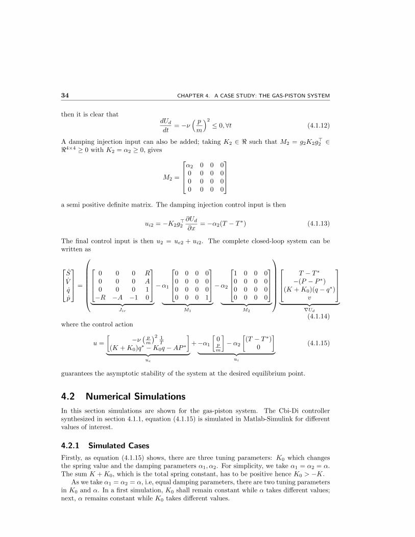
34 CHAPTER 4. A CASE STUDY: THE GAS-PISTON SYSTEM
then it is clear thatdUddt
= −ν( pm
)2
≤ 0,∀t (4.1.12)
A damping injection input can also be added; taking K2 ∈ < such that M2 = g2K2g>2 ∈
<4×4 ≥ 0 with K2 = α2 ≥ 0, gives
M2 =
α2 0 0 00 0 0 00 0 0 00 0 0 0
a semi positive definite matrix. The damping injection control input is then
ui2 = −K2g>2
∂Ud∂x
= −α2(T − T ∗) (4.1.13)
The final control input is then u2 = ue2 + ui2. The complete closed-loop system can bewritten as
S
Vqp
=
0 0 0 R0 0 0 A0 0 0 1−R −A −1 0
︸ ︷︷ ︸
Jir
−α1
0 0 0 00 0 0 00 0 0 00 0 0 1
︸ ︷︷ ︸
M1
−α2
1 0 0 00 0 0 00 0 0 00 0 0 0
︸ ︷︷ ︸
M2
T − T ∗−(P − P ∗)
(K +K0)(q − q∗)v
︸ ︷︷ ︸
∇Ud
(4.1.14)where the control action
u =
[−ν(pm
)2 1T
(K +K0)q∗ −K0q −AP ∗]
︸ ︷︷ ︸ue
+−α1
[0pm
]− α2
[(T − T ∗)
0
]︸ ︷︷ ︸
ui
(4.1.15)
guarantees the asymptotic stability of the system at the desired equilibrium point.
4.2 Numerical Simulations
In this section simulations are shown for the gas-piston system. The Cbi-Di controllersynthesized in section 4.1.1, equation (4.1.15) is simulated in Matlab-Simulink for differentvalues of interest.
4.2.1 Simulated Cases
Firstly, as equation (4.1.15) shows, there are three tuning parameters: K0 which changesthe spring value and the damping parameters α1, α2. For simplicity, we take α1 = α2 = α.The sum K +K0, which is the total spring constant, has to be positive hence K0 > −K.
As we take α1 = α2 = α, i.e, equal damping parameters, there are two tuning parametersin K0 and α. In a first simulation, K0 shall remain constant while α takes different values;next, α remains constant while K0 takes different values.
4.2. NUMERICAL SIMULATIONS 35
4.2.2 Simulation Values
Table 4.1 shows the parameters which describes the Gas-Piston system with its simulationvalues. The control objective is the volume and entropy of the piston, with a desired volumeof V ∗ = 0.03[m3] which gives q∗ = 0.6[m]; momentum p∗ = 0[Kg·m/s] and a desired entropyof S∗ = 30[J/K].
Numerical values were taken from general applications that include electric generators,hydraulic pumps and air compressors [18] while thermodynamics values were taken from [8].
4.2.3 Simulation Results
This section shows the simulation results with the simulation values of section 4.2.2.Figure 4.2 and 4.3 show the state variables of the system for different α values, and
different K0 values, respectively. The objective variables are the volume and the entropy ofthe system. The plot shows the entropy S of the system; the volume V of the piston andthe momentum p. We didn’t explicit show the position of the piston as this variable has alinear behaviour with the volume of the piston.
The K0 parameter, which varies in figure 4.3 and which is related to the closed-loopHamiltonian function, shows that there is a trade off between the speed of the closed-loopsystem and the oscillation of the states. The input u2 in figure 4.5, when K0 is moving,shows that as K0 increases more energetic inputs we get; this is natural as more energeticinputs are needed in order for the closed-loop to converge faster.
The entropy of the system, otherwise, has no relation with the tuning parameter K0
which is shown in input u1, figure 4.4 when α = 1. This is no surprise as the control actionacting on the entropy is entirely due to the heat flux.
The damping injection coefficient α is in charge of the asymptotic stability of the systemaccording to proposition 3; figure 4.2 shows the response of the system for different αvalues. An increase of α produces a faster response on the dynamics of the system; as aresult, the control objective is reached faster. See, for example, the entropy, the volume andthe momentum of the system for α = 10. For this particular value, input u1, u2 in figures4.4,4.5 with K0 = 0, show that as expected, inputs with faster initial response are neededto guarantee a faster response of the closed-loop system.
The choice of α and K0 depends on the control requirements. If a faster response of theclosed-loop system is required, with no particular need of a low magnitude input, then ahigh damping value should be selected.
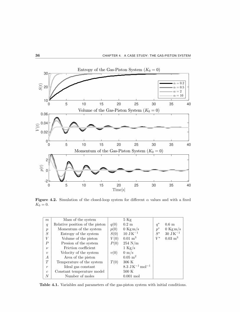
36 CHAPTER 4. A CASE STUDY: THE GAS-PISTON SYSTEM
0 5 10 15 20 25 30 35 4010
20
30
0 5 10 15 20 25 30 35 400
0.02
0.04
0.06
0 5 10 15 20 25 30 35 40
-2
0
2
Figure 4.2. Simulation of the closed-loop system for different α values and with a fixedK0 = 0.
m Mass of the system 5 Kgq Relative position of the piston q(0) 0.2 m q∗ 0.6 mp Momentum of the system p(0) 0 Kg m/s p∗ 0 Kg m/sS Entropy of the system S(0) 10 J K−1 S∗ 30 J K−1
V Volume of the piston V (0) 0.01 m3 V ∗ 0.03 m3
P Presion of the system P (0) 254 N/mν Friction coefficient 1 Kg/sv Velocity of the system v(0) 0 m/sA Area of the piston 0.05 m2
T Temperature of the system T (0) 306 Kr Ideal gas constant 8.3 J K−1 mol−1
c Constant temperature model 500 KN Number of moles 0.001 mol
Table 4.1. Variables and parameters of the gas-piston system with initial conditions.
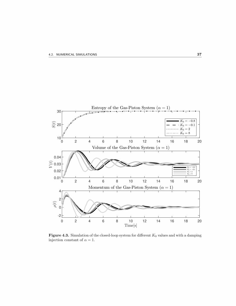
4.2. NUMERICAL SIMULATIONS 37
0 2 4 6 8 10 12 14 16 18 2010
20
30
0 2 4 6 8 10 12 14 16 18 200.01
0.02
0.03
0.04
0 2 4 6 8 10 12 14 16 18 20
-2
0
2
4
Figure 4.3. Simulation of the closed-loop system for differentK0 values and with a dampinginjection constant of α = 1.
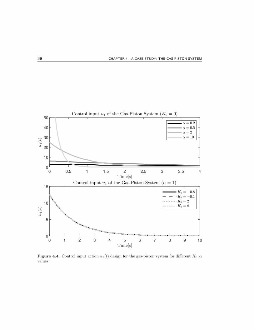
38 CHAPTER 4. A CASE STUDY: THE GAS-PISTON SYSTEM
0 0.5 1 1.5 2 2.5 3 3.5 40
10
20
30
40
50
0 1 2 3 4 5 6 7 8 9 100
5
10
15
Figure 4.4. Control input action u1(t) design for the gas-piston system for different K0, αvalues.
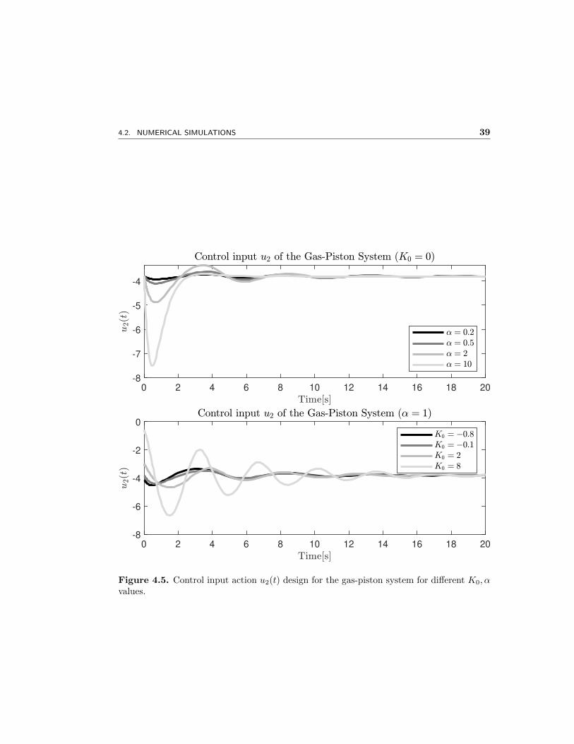
4.2. NUMERICAL SIMULATIONS 39
0 2 4 6 8 10 12 14 16 18 20-8
-7
-6
-5
-4
0 2 4 6 8 10 12 14 16 18 20-8
-6
-4
-2
0
Figure 4.5. Control input action u2(t) design for the gas-piston system for different K0, αvalues.
Chapter 5
CONCLUSION
This thesis considers the problem of passivity based control (PBC) of irreversible portHamiltonian systems (IPHS) which are an extension of the port Hamiltonian system (PHS)framework for irreversible thermodynamic. The control design is based on the classicalPBC techniques for PHS such as control by interconnection (Cbi) and damping injection(Di). To this purpose, an IPHS is controlled with a double control loop; the first loop isin charge of the stability of the system by shaping the Hamiltonian energy function withan energy shaping control design approach, where the Cbi is done by considering an IPHScontroller. In order to achieve this, the existence of Casimir functions, which relate thestates of the system and the controller, are fundamental. The result is a set of partialdifferential equations whose solutions are the Casimir functions of the system. The energyshaping controller then shapes the Hamiltonian energy of the closed-loop into a desiredenergy function.
The second control loop guarantees the asymptotic stability of the system, through adamping injection control action.
The result is then a controller which achieves asymptotic stability at a desired equilibriumdynamic in the closed-loop system.
A proposition that summarize the Cbi-Di control for IPHS is given. Furthermore, aCbi-Di controller is obtained for a CSTR system as an illustrative example and the corre-spondence of the controller with previously reported results using IDA-PBC is established.
A controller for a gas-piston system, which is a complex coupled mechanic-themodynamicprocess, is synthesized and simulations for the system show the performance of the controller.The closed-loop system is asymptotically stable and numerical simulations illustrate howthe entropy of the system, which represents the irreversibility of the process, follows thereference with a tuning parameter which determines the speed of the closed-loop systemresponse.
5.1 Future Work
As the present thesis extends the Cbi-Di control for irreversible-reversible processes, an im-portant application for future work is related to the control of micro-mechanical systemswith hysteresis, where piezoelectric systems are of particular interest and others coupledmechanical-thermodynamical systems. Also, it would be interesting to compare the perfor-mance of the Cbi-Di controllers with other frameworks for control of irreversible-reversiblesystems.
Numerical simulations for the CSTR systems are also important, with the applicationof the method, for example, to a Van Der Vusse Reactor ([34], [24]).
40
REFERENCES
[1] Antonio A. Alonso and B.Erik Ydstie. Stabilization of distributed systems using irre-versible thermodynamics. Automatica, 37(11):1739 – 1755, 2001.
[2] Rutherford Aris. Elementary chemical reactor analysis. Butterworths Series in ChemicalEngineering, 1989.
[3] Karl Johan Astrom and Bjorn Wittenmark. Adaptive Control. Addison-Wesley LongmanPublishing Co., Inc., USA, 2nd edition, 1994.
[4] H. Callen. Thermodynamics and an introduction to thermostatistics. Wiley, New-York,1985.
[5] Daizhan Cheng. Generalized Hamiltonian Systems, pages 1–51. 2001.
[6] Daizhan Cheng, Tielong Shen, and Tzyh Jong Tarn. Pseudo-hamiltonian realization andits application. Communications in Information and Systems, 2:91–120, 01 2003.
[7] F. Couenne, C. Jallut, B. Maschke, P.C. Breedveld, and M. Tayakout. Bond graph mod-elling for chemical reactors. Mathematical and Computer Modelling of Dynamical Systems,12(2-3):159–174, April 2006.
[8] I. Prigogine D. Kondepudi. John Wiley & Sons, New York, 1998.
[9] Cheng Daizhan, Xue Weimin, Liao Lizhi, and Cai Dayong. On generalized hamiltoniansystems. Acta Mathematicae Applicatae Sinica, 17(4):475–483, Oct 2001.
[10] Vincent Duindam, Alessandro Macchelli, Stefano Stramigioli, and Herman Bruyninckx.Modeling and Control of Complex Physical Systems: The Port-Hamiltonian Approach. 012009.
[11] D. Eberard, B. Maschke, and A.J. van der Schaft. Conservative systems with ports oncontact manifolds. IFAC Proceedings Volumes, 38(1):342 – 347, 2005. 16th IFAC WorldCongress.
[12] D. Eberard, B. M. Maschke, and A. J. van der Schaft. Port contact systems for irre-versible thermodynamical systems. In Proceedings of the 44th IEEE Conference on Decisionand Control, pages 5977–5982, 2005.
[13] A. Favache and D. Dochain. Thermodynamics and chemical systems stability: The cstrcase study revisited. Journal of Process Control, 19(3):371 – 379, 2009.
41
42 References
[14] Miroslav Grmela and Hans Ottinger. Dynamics and thermodynamics of complex fluids.i. development of a general formalism. Phys. Rev. E, 56, 12 1997.
[15] Wassim M. Haddad and VijaySekhar Chellaboina. Nonlinear Dynamical Systems andControl: A Lyapunov-Based Approach. Princeton University Press, 2008.
[16] H. Hoang, F. Couenne, C. Jallut, and Y. Le Gorrec. The port Hamiltonian approachto modeling and control of continuous stirred tank reactors. Journal of Process Control,21(10):1449 – 1458, 2011.
[17] H. Hoang, F. Couenne, C. Jallut, and Y. Le Gorrec. Lyapunov-based control of nonisothermal continuous stirred tank reactors using irreversible thermodynamics. Journal ofProcess Control, 22(2):412 – 422, 2012.
[18] Boru Jia, Andrew Smallbone, Huihua Feng, Guohong Tian, Zhengxing Zuo, and A.P.Roskilly. A fast response free-piston engine generator numerical model for control applica-tions. Applied Energy, 162:321 – 329, 2016.
[19] Kendell R. Jillson and B. Erik Ydstie. Process networks with decentralized inventoryand flow control. Journal of Process Control, 17(5):399 – 413, 2007.
[20] Robert Jongschaap and Hans Christian Ottinger. The mathematical representation ofdriven thermodynamic systems. Journal of Non-Newtonian Fluid Mechanics, 120(1):3 – 9,2004. 3rd International workshop on Nonequilibrium Thermodynamics and Complex Fluids.
[21] B.M. Maschke, A.J. Van Der Schaft, and P.C. Breedveld. An intrinsic Hamiltonianformulation of network dynamics: non-standard poisson structures and gyrators. Journalof the Franklin Institute, 329(5):923 – 966, 1992.
[22] B.M. Maschke and A.J. van der Schaft. Port-controlled hamiltonian systems: Modellingorigins and system theoretic properties. IFAC Proceedings Volumes, 25(13):359 – 365, 1992.2nd IFAC Symposium on Nonlinear Control Systems Design 1992, Bordeaux, France, 24-26June.
[23] W. Muschik, S. Gumbel, M. Kroger, and H. C. Ottinger. A simple example for comparingGENERIC with rational non-equilibrium thermodynamics. Physica A Statistical Mechanicsand its Applications, 285(3):448–466, Oct 2000.
[24] Michael Niemiec and Costas Kravaris. Nonlinear model-state feedback control fornonminimum-phase processes. Automatica, 39:1295–1302, 07 2003.
[25] R. Ortega, A. van der Schaft, B. Maschke, and G. Escobar. Energy-shaping of port-controlled hamiltonian systems by interconnection. In Proceedings of the 38th IEEE Con-ference on Decision and Control (Cat. No.99CH36304), volume 2, pages 1646–1651 vol.2,1999.
[26] Romeo Ortega and Eloısa Garcıa-Canseco. Interconnection and damping assignmentpassivity-based control: A survey. European Journal of Control, 10(5):432 – 450, 2004.
[27] Romeo Ortega, Arjan van der Schaft, and Bernhard M. Maschke. Stabilization of port-controlled hamiltonian systems via energy balancing. In Stability and Stabilization of Non-linear Systems, pages 239–260, London, 1999. Springer London.
References 43
[28] Hans Christian Ottinger. Nonequilibrium thermodynamics–a tool for applied rheologists.Applied Rheology, 9(1):17–26, 1999.
[29] Hans Christian Ottinger and Miroslav Grmela. Dynamics and thermodynamics of com-plex fluids. ii. illustrations of a general formalism. Phys. Rev. E, 56:6633–6655, Dec 1997.
[30] I Prigogine and R Defay. Treatise on thermodynamics. Chemical thermodynamics.London, Great Britain: Longmans Green and Co, 1, 1954.
[31] Hector Ramırez, Yann Le Gorrec, Bernhard Maschke, and Francoise Couenne. On thepassivity based control of irreversible processes: A port-Hamiltonian approach. Automatica,64:105 – 111, 2016.
[32] Hector Ramırez, Bernhard Maschke, and Daniel Sbarbaro. Irreversible port-Hamiltoniansystems: A general formulation of irreversible processes with application to the cstr. Chem-ical Engineering Science, 89:223 – 234, 2013a.
[33] Hector Ramırez, Bernhard Maschke, and Daniel Sbarbaro. Modelling and control ofmulti-energy systems: An irreversible port-Hamiltonian approach. European Journal ofControl, 19(6):513 – 520, 2013b.
[34] Hector Ramırez, Daniel Sbarbaro, and Romeo Ortega. On the control of non-linearprocesses: An ida-pbc approch. Journal of Process Control, 19:405–414, 03 2009.
[35] Arjan van der Schaft. Port-controlled hamiltonian systems: Towards a theory for controland design of nonlinear physical systems. Journal of The Society of Instrument and ControlEngineers, 39, 02 2000.
[36] Arjan van der Schaft. Port-Hamiltonian systems: network modeling and control of non-linear physical systems, pages 127–167. Springer, 2004.
[37] Arjan van der Schaft. L2-Gain and Passivity Techniques in Nonlinear Control. SpringerPublishing Company, Incorporated, 3rd edition, 2016.
[38] Arjan van der Schaft and Dimitri Jeltsema. Port-Hamiltonian systems theory: Anintroductory overview. Foundations and Trends R© in Systems and Control, 1(2-3):173–378,2014.
[39] B.Erik Ydstie. Passivity based control via the second law. Computers & ChemicalEngineering, 26(7):1037 – 1048, 2002.