Passivity based Supervisory Control

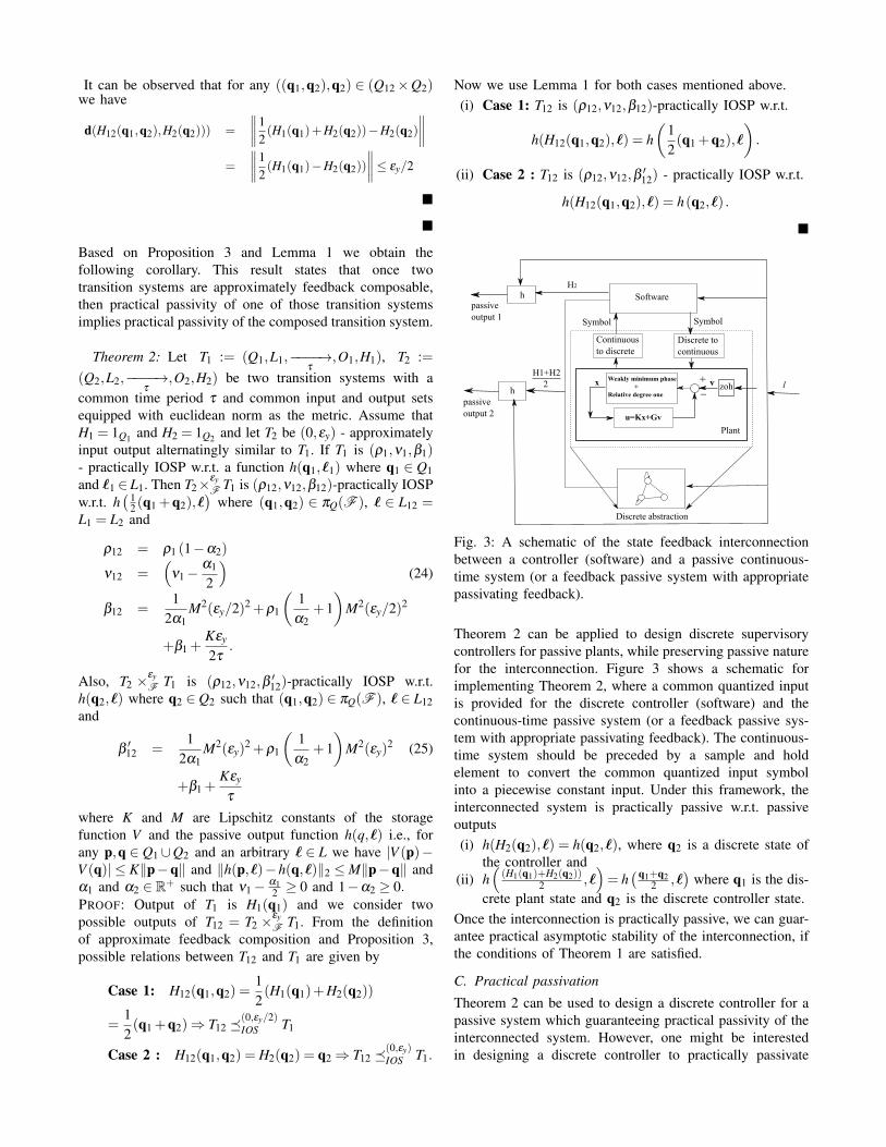
Passivity based Supervisory Control

Technical Report of the ISIS Groupat the University of Notre Dame

ISIS-2014-005July 2014

(Revised in March 2015)

S. Sajja, V. Gupta, and P.J. AntsaklisDepartment of Electrical Engineering

University of Notre DameNotre Dame, IN 46556

Interdisciplinary Studies in Intelligent Systems

Acknowledgements The support of the National Science Foundationunder the CPS Grant No. CNS-1035655 is gratefully acknowledged.

On a notion of passivity for discrete systems

Shravan Sajja1∗, Vijay Gupta2 and Panos J. Antsaklis2

Abstract— Cyber Physical Systems (CPS) often have contin-uous components interconnected with systems described bydiscrete state space. Examples of such discrete componentsmay be supervisory controllers or components implemented insoftware. To design large scale CPS in a compositional mannerit would be useful to define a notion of passivity for thesediscrete components as well. As a first step towards this goalwe assign notions of passivity and passivity indices for a finitestate model that is abstracted from an infinite state continuoussystem. We also characterize the degradation of passivity underthis abstraction and analyze the stability properties of suchpassive discrete systems.

I. INTRODUCTION

There is a resurgence of interest in the classical conceptsof passivity and dissipativity for the design of largescale cyber physical systems owing to the property ofcompositionality that these concepts offer. The readeris referred to texts such as [1], [2] and articles such as[3], [4] for a survey of the research landscape in thisdirection. Somewhat surprisingly, however, there is limitedunderstanding of passivity for discrete (state) systems,such as those obtained when systems are implemented insoftware or from higher order controllers such as supervisorycontrollers or trajectory planners.

Interaction between continuous plants and discretecontrollers is an important feature of modern day embeddedsystems and cyber physical systems. The problem isnot trivial since it is known that several conventionaldiscretization methods (where discretization is of thetime variable and the state is deemed continuous) andquantization procedures (quantization of input and output)degrade passivity, and more generally, dissipativityproperties of a continuous-time system [5]. Hence carefuldesign of sampling time, input and output signals, orquantization methods is needed to ensure passivity [6],[7], [8]. The problem is even more difficult when thestate is discretized (as in a finite state model) or when adiscrete supervisor is interconnected with a continuous plant.

A relevant line of research is passivity of hybrid systemswhere both continuous and discrete dynamics are consideredin the same framework [9], [10]. Recently, new passivityconditions have also been proposed for switched systems

*This work was done when author was in Department of ElectricalEngineering, University of Notre Dame, Notre Dame, IN 46556, USA

1 Author is with IBM Research Dublin, [email protected]

2 Authors are with the Department of Electrical Engineering,University of Notre Dame, Notre Dame, IN 46556, [email protected], [email protected]

[11], linear complimentarity systems [12] and piecewiseaffine systems [13]. Although the hybrid systems frameworkis well established, systematic compositional methods toanalyze the interconnection between discrete controllers andcontinuous plants are not yet available.

Instead, we follow an alternate approach based onabstracting finite state models from infinite state models(continuous-time systems) which may further interact withother finite state systems. There is now significant workavailable on abstracting finite state models from continuoussystems while maintaining equivalence in a certain sensebetween the two [14], [15] , [16], [17]. The commonapproach between most of these works is to design discretecontrollers for the finite state discrete abstractions of aplant in order to satisfy given discrete specifications. Theabstractions are such that the same discrete controller worksfor the continuous system. This requirement imposes certainrequirements on the abstraction methodology in order tomaintain a certain equivalence between the continuoussystems and the finite state systems. In works such as [17],[18], notions of input output stability and Lyapunov stabilityhave been proposed for systems in the discrete domain;however, they do not allow a natural description of system’spassive behavior. Passivity property for continuous plantsis described using a notion of inner product over a realspace, thus motivating abstractions which allow a notion ofinner product to defined for the input-output vectors of thefinite state abstraction. To this end, we follow the approachof abstracting a finite state model using the concepts ofsimulations and bisimulations. In particular, we followthe notions of approximate simulation and approximatebisimulation [19], and in particular their extensions forcontinuous nonlinear systems that are incrementally forwardcomplete [20].

Specifically, we note that [20] incorporates notions of ametric and a vector space, as well as provides us conditionson sampling time and quantization parameters that guaranteeapproximately similar models. The notions of approximatesimilarity are based on bounding the distance between theoutput trajectories of the continuous-time system and itsabstraction. However, in order to preserve properties likepassivity, which are described using both inputs and outputs,we need to extend the notions of approximate simulationfurther. In Section II we introduce new notions of ap-proximate input output simulation and approximate inputoutput alternating simulation. Similar notions of input outputsimulations were also proposed by [23] and [24]. In Section

III, we show how to obtain such finite abstractions basedon certain modifications to the methods proposed by [20].Then we use these approximate relations to quantify thedegradation of passivity (in terms of passivity indices) underabstraction. In Section IV, we generalize notions of passivityand dissipativity for a class of finite state transition systems.Then we analyze such finite abstractions to find conditionsunder which they attain stable behavior in a practical sense.A companion paper [29] considers the interaction of thesefinite state models with higher order supervisory controllersto ensure that the entire interconnection is passive. Wewould also like to mention the paper [30] that considersthe related but complementary problem of discretizing acontroller designed in the continuous space so that passivityindices of the closed loop system are maintained despitediscretization. Note that while [30] requires a bisimulationof the controller, we require a simulation of the plant for ourpurpose.

II. PRELIMINARIES

A. Notation

The identity map on a set A is denoted by 1A. If A is asubset of B we denote by ıA : A ↪→ B or simply by ı thenatural inclusion map taking any a ∈ A to ı(a) = a ∈ B. Thesymbols N, R, R+ and R+

0 denote the set of natural, real,positive, and nonnegative real numbers, respectively. Thetranspose of a general matrix M is denoted by MT . A matrixP is symmetric if PT = P. A symmetric matrix P is positive(negative) definite if xT Px > 0 (xT Px < 0) for all non-zero xand we denote this by P > 0 (P < 0). A symmetric matrixP is positive (negative) semi-definite if xT Px≥ 0 (xT Px≤ 0)for all x and we denote this by P ≥ 0 (P ≤ 0). The innerproduct of signals u(t), y(t) is denoted by 〈u,y〉 defined as〈u,y〉 =

∫ t0 uT (τ)y(τ)dτ . Given a vector x ∈ Rn, xi is the i-

th element of x and we denote infinity norm and euclideannorms of x by ‖x‖ and ‖x‖2. Given a measurable functionf : R+ : 0← Rn the (essential) supremum (sup norm) of fis denoted by ‖‖∞. If A⊆ Rn and η ∈ R+, [A]η denotes thesubset [A]η ⊆ A defined by:

[A]η ={

z ∈ A | zi = kiη for some ki ∈ A and i = 1,2, . . . ,n}.

The set [A]η will be used as an approximation of the set Awith precision η . If we define Bε(x) = {y ∈ Rn| ‖x− y‖ ≤ε}. For set A ⊆ Rn of the form A =

⋃Mj=1 A j for some

M ∈ N, where A j = Πni=1[c

ji ,d

ji ] ⊆ Rn with c j

i < d ji and

positive constant η ≤ η , where η = min j=1,...,M ηA j andηA j = min{|d j

1− c j1|, · · · , |d

jn− c j

n|}. Note that [A]η 6= ∅ forany η ≤ η . Geometrically, for any η ∈ R+ and λ ≥ η

the collection of sets {Bλ (p)}p∈[A]η is a covering of A,i.e. A⊆

⋃p∈[A]η Bλ (p). A continuous function γ : R+

0 → R+0

belongs to class K if it is strictly increasing and γ(0) = 0;γ belongs to class K∞ if γ ∈K and γ(r)→ ∞ as r→ ∞.A continuous function γ : R+

0 ×R+0 → R+

0 belongs to classK L if, for each fixed s, the map β (r,s) belongs to classK∞ with respect to r and, for each fixed r, the map β (r,s)is decreasing with respect to s and β (r,s)→ 0 as s→ ∞. A

relation R⊆A×B is defined by a map of the form R : A→ 2B

where b ∈ R(a) if and only if (a,b) ∈ R. For a set S ∈ A theset R(S) is defined as R(S) = {b ∈ B : ∃ a ∈ S,(a,b) ∈ R}.We also denote by d : X×X →R+

0 a metric in the space X .

B. Incremental forwardness and stability

In this paper we restrict ourselves to control systems of theform Σ = (Rn,U,U , f ) where• Rn is the state space;• U⊆ Rm is the input space;• U :R→U is a subset of the set of all locally essentially

bounded functions of time from intervals of the form]a,b[⊆ R to U with a < 0 and b > 0;

• f : Rn×U→ Rn is a Lipschitz continuous map.If ξ :]a,b[−−→ Rn is a trajectory of Σ (or equivalently asolution of the differential equation x = f (x,u)), then wewill use ξ (τ,x,v) to denote a unique point reached at timeτ under the input v from an initial condition x. System Σ issaid to be forward-complete if such a solution is defined forall t ∈]0,∞[. In this paper we use an incremental version ofthis property, defined as:

Definition 1 (Incremental forward-completeness): Acontrol system Σ is δ -FC if there exist continuous functionsβ : R+

0 ×R+0 → R+

0 and γ : R+0 ×R+

0 → R+0 such that for

every s∈R+, the functions β (·,s) and γ(·,s) belong to classK∞, and for any x,x′ ∈ Rn, any τ ∈ R+, and any v,v′ ∈U ,where v,v′ : [0,τ)→ U, the following condition is satisfiedfor all t ∈ [0,τ]:

‖ξ (t,x,v)−ξ (t,x′,v′)‖ ≤ β (‖x− x′‖, t)+ γ(‖v− v′‖∞, t).(1)

Definition 2 (Asymptotic Stability): The origin of Σ withx = f (x,0) is asymptotically stable if and only if there existsa β (·, ·) ∈K L such that when ‖x(0)‖ ≤ δ we have

‖ξ (t,x(0),0)‖ ≤ β (‖x(0)‖, t) ∀t ≥ 0. (2)

C. Dissipativity

Consider the system Σ and an output function y = h(x,u) ∈Rp. Further, assume that f (0,0) = 0 and h(0,0) = 0. Σ isdissipative w.r.t. y = h(x,u) if there exists a C 1 storagefunction V (x) : Rn→R+

0 and a supply rate ω : U×Rp→R+0

such that V (0) = 0 and the following inequality is satisfied:

V (x(t))−V (x(t0))≤∫ t

t0ω(u,y)dt (3)

for any t ≥ t0 and u ∈U . A special case of dissipativity is(ρ,ν)-input output strict passivity (IOSP) when ω(u,y) =uT y−νuT u−ρyT y with ρ,ν ≥ 0. In this definition, parame-ters ν and ρ are known as passivity indices. The next Lemmapresents an important implication of passivity on stabilityproperties of Σ.

Lemma 1: [25](Zero-input asymptotic stability) Theorigin of Σ with x = f (x,0) is asymptotically stable ifΣ is (ρ,ν) - IOSP with ρ > 0 and ν ≥ 0 and ρyT y > 0.Furthermore, if the storage function is radially unbounded,the origin will be globally asymptotically stable.

One of our main goals in this paper is to understandthe implications of finite state abstraction on such stabilityproperties of a passive system.

D. Transition systems and system relations

Definition 3: [21] A system T is a quintuple T =(X ,U,−−→,Y,H) consisting of:

• A set of states X ;• A set of inputs U ;• A transition relation −−→⊆ X×U×X ;• An output set Y ;• An output function H : X → Y .

T is said to be metric, if the output set Y is equipped witha metric; d : Y ×Y → R+

0 . To define notions of stability fortransition systems we assume that the finite sets X ,U , and Yare equipped with the metric given by d(x,y)= ‖x−y‖ wherex,y are elements of X ,U , or Y . If for any state x ∈ X andu∈U there exists at most one state x′ ∈ X such that x u−−−→x′. If the system is nondeterministic, then for a transitionx u−−−→ x′ the state x′ may not unique, x′ is also known asthe u-successor of x. In such a case x′ belongs to a set ofall possible u-successors given by Postu(x) and we will useU(x) to denote the set of inputs u ∈U for which Postu(x)is nonempty. We will further use Postu(Q) to denote the set⋃

x∈Q Postu(x).

E. System relations

Now we present certain system relations, that are essentialin obtaining faithful finite abstractions for control systems.Approximate simulation relations used in [19] and [22]are primarily based on bounding the distance between theoutputs or states of the continuous-time and its abstraction.However, in order to account for behaviors like passivity(which are defined using both inputs and outputs), we in-troduce new notions of approximate input output simulationand approximate input output alternating simulation.

Definition 4 (Approximate input output simulation):Let T1 := (X1,U1,−−−−→

1,Y1,H1), T2 := (X2,U2,−−−−→

2,Y2,H2) be metric transition systems with the same sets ofinputs U = U1 = U2 and outputs Y = Y1 = Y2 and equippedwith the metric d. Let εu,εy ∈ R+

0 be given precisionrequirements then a relation R ⊆ X1×X2 is said to be an(εu,εy) - approximate input output simulation (IOS) relationbetween T1 and T2 if the following two conditions aresatisfied:(i) for every (x1,x2) ∈ R we have d(H1(x1),H2(x2))≤ εy;

(ii) for every (x1,x2) ∈ R and for every u1 ∈U1 there existsu2 ∈U2 such that d(u1,u2)≤ εu and x1

u1−−−−→1

x′1 in T1

implies the existence of x2u2−−−−→2

x′2 in T2 such that

(x′1,x′2) ∈ R.

Definition 5: (Approximate input output alternatingsimulation): Let T1 := (X1,U1,−−−−→

1,Y1,H1), T2 :=

(X2,U2,−−−−→2

,Y2,H2) be metric transition systems with thesame sets of inputs U = U1 = U2 and outputs Y = Y1 = Y2

and equipped with the metric d. Let εu,εy ∈ R+0 be a given

precision requirements, a relation R ⊆ X1×X2 is said to bean (εu,εy) - approximate input output alternating simulation(IOAS) relation from T1 to T2 if condition (i) of Definition4 and the following condition are satisfied:(iii) for every (x1,x2) ∈ R and for every u1 ∈U1(x1) there

exists u2 ∈U2(x2) such that d(u1,u2)≤ εu and for everyx′2 ∈ Postu2(x2) there exists x′1 ∈ Postu1(x1) satisfying(x′2,x

′1) ∈ R.

The two notions of alternating approximate simulation andapproximate simulation coincide in the special case of de-terministic systems. If T1 is (εu,εy)- approximately inputoutput simulated (or approximately input output alternatinglysimulated) by T2, then we denote this fact by T1 �

(εu,εy)IOS T2

(T1 �(εu,εy)IOAS T2).

F. Finitely abstracted transition systems

In this paper, we make a modification to the proceduredescribed in [20], to obtain finite state transition systems.Method described in [20] is based on selection of appropriatesampling time and quantization parameters which guaranteeapproximate simulation and alternating simulation relationsbetween the original system and its abstraction. Initiallywe consider a discrete time sub-transition system Tτ(Σ)corresponding to Σ = (Rn,U,U , f ) with a sampling timeperiod τ ∈ R+. We further assume that control inputs arepiecewise-constant over the sampling time period τ , the classof inputs considered are:

Uτ := {u ∈U | u(t) = u(0), t ∈ [0,τ]}.

For Tτ(Σ) we use identity map as the output function,however, for stability and passivity analysis, we use analternate output corresponding to y = h(x,u).

Definition 6: [21] Let Σ be a control system and T (Σ) itsassociated transition system. For any τ > 0, the sub transitionsystem Tτ(Σ) := (Xτ ,Uτ ,

uτ−−−−→τ

,Yτ ,Hτ) is defined by:

• Xτ = Rn;• Uτ = Uτ ;• xτ

uτ−−−−→τ

x′τ , if there exists a trajectory ξ : [0,τ]−−−→ξ (τ,xτ ,uτ) = x′τ ;

• Yτ = Rn;• Hτ = 1Rn .

Now we restrict the input set and the state set to a hyper-rectanlges U⊆Rm and X ⊆Rn such that {0} ∈U and {0} ∈X . Then we choose input and state quantization factors suchthat µ ≤ µ and η ≤ η (see Section II.A on how to calculateµ , η).

Definition 7: For any δ -FC control system Σ and parame-ters τ > 0, η > 0, µ > 0 and a design parameters θ1,θ2 ∈R+,a countable transition system can be defined as:

Tτ,µ,η(Σ) := (Xq,Uq,uq−−−−→τ

,Yq,Hq) (4)

where:• Xq = [X ]η ;• Uq = [U]µ ;

• xquq−−−−→τ

x′q, if ‖ξ (τ,xq,uq) − x′q‖ ≤ β (θ1,τ) +

γ(θ2,τ)+η ;• Yq = [X ]η• Hq = ı : Xq ↪→ Yq

where β and γ are functions from Definition 1.Finite transition system Tτ,µ,η(Σ) is different from the tran-sition systems abstracted in [20], because of an extra designparameter θ2. This extra design parameter is necessary toobtain finite abstractions which are approximately inputoutput (alternatingly) similar to the original system. In thenext section we provide sufficient conditions to guarantee theexistence of such approximate abstractions. We also quantifythe degradation of passivity condition for a continuous-time IOSP system under such abstractions. We illustrate thisdegradation through a new dissipation inequality satisfiedby the finitely abstracted transition system. Based on thisnew inequality, we define a new notion of practical passivityfor transition systems. Further, we show that this notion ofpractical passivity guarantees a notion of zero-input practicalasymptotic stability transition system akin to continuous-timepassive systems.

III. DEGRADATION OF PASSIVITY

Initially we provide sufficient conditions for Tτ,η ,µ(Σ) to be(εu,εy) - approximately input output (alternatingly) similarTτ(Σ).

Proposition 1: Consider a control system Σ and any de-sired precision parameters εy > 0, εu > 0. If Σ is δ -FC thenfor any τ > 0, θ1 > 0, θ2 > 0, η > 0 and µ > 0 satisfyingthe following inequality:

β (θ1,τ)+ γ(θ2,τ)+η ≤ εy, (5)

such that η ≤ εy ≤ θ1 and µ ≤ εu ≤ θ2, we have:

Tτ,η ,µ(Σ)�(εu,εy)IOAS Tτ(Σ)�

(εu,εy)IOS Tτ,η ,µ(Σ). (6)

PROOF: Initially we show that Tτ(Σ)�(εu,εy)IOS Tτ,η ,µ(Σ). Con-

sider any xτ ∈ Xτ and uτ ∈Uτ , then there exists xq ∈ Xq =[X ]η and uq ∈Uq = [U]µ such that

‖xτ − xq‖ ≤ η ≤ εy (7)

and‖uτ −uq‖ ≤ µ ≤ εu (8)

This is possible because of the nature of quantization whichallows Xτ ⊆

⋃p∈[X ]η Bλ (p) and Uτ ⊆

⋃p∈[U]µ Bλ (p). From

the definitions of output functions Hτ = 1Rn and Hq = ı :Xq ↪→ Yq, we have ‖Hτ(xτ)− Hq(xq)‖ = ‖xτ − xq‖ ≤ εu,hence condition (i) of Definition 4 is satisfied.

Now if we consider the transition xτ

uτ−−−−→τ

x′τ in thetransition system Tτ(Σ) , then the distance between x′τ andξ (τ,xq,uq) can estimated based on the δ - FC property ofΣ and inequalities (7) and (8) i.e.,

‖x′τ −ξ (τ,xq,uq)‖ ≤ β (εy,τ)+ γ(εu,τ) (9)

Since Xτ ⊆⋃

p∈[X ]η Bλ (p), there exists x′q ∈ Xq such that

‖x′τ − x′q‖ ≤ η (10)

From the triangular inequality we have

‖ξ (τ,xq,uq)− x′q‖ ≤ ‖ξ (τ,xq,uq)− x′τ‖+‖x′τ − x′q‖

From inequalities (9) and (10) we have

‖ξ (τ,xq,uq)− x′q‖ ≤ β (εy,τ)+ γ(εu,τ)+η

Finally we use η ≤ εy ≤ θ1 and µ ≤ εu ≤ θ2 to show that

‖ξ (τ,xq,uq)− x′q‖ ≤ β (θ1,τ)+ γ(θ2,τ)+η

which, by the definition of Tτ,µ,η(Σ) implies the existenceof xq

uq−−−→ x′q in Tτ,µ,η(Σ). Therefore, from inequality(10) and since η ≤ εy we conclude that (x′τ ,x

′q) ∈ R and

condition (ii) in Definition 4 holds.

Now we show that Tτ,η ,µ(Σ)�(εu,εy)IOAS Tτ(Σ). For R⊆ Xτ ×Xq

we consider an xτ = xq ∈ Xq. This is possible becauseXq ⊆ Xτ and it satisfies condition (i) of Definition 4 (i.e.,‖xτ − xq‖= 0 < εy). Now we choose an input uτ = uq ∈Uq(satisfying ‖uτ−uq‖= 0 < εu) and consider the unique tran-sition xτ

uτ−−−−→τ

x′τ = ξ (τ,xτ ,uτ) ∈ Postuτ(xτ). The distance

between x′τ and ξ (τ,xq,uq) can be bounded using the δ -FC properties of Σ, i.e.,

‖x′τ −ξ (τ,xq,uq)‖ ≤ β (0,τ)+ γ(0,τ) (11)

Since Xτ ⊆⋃

p∈[X ]η Bλ (p), we can always find x′q ∈ Xq suchthat

‖x′q− x′τ‖ ≤ η (12)

From the triangular inequality and inequalities (11) and (12)we have

‖ξ (τ,xq,uq)− x′q‖ ≤ ‖ξ (τ,xq,uq)− x′τ‖+‖x′τ − x′q‖≤ β (0,τ)+ γ(0,τ)+η

Finally we use 0 < θ1 and 0 < θ2 to show that




′q) ∈ R and

condition (iii) in Definition 5 holds.

�

Now we analyze degradation of passivity of Σ under ap-proximate input output similarity. For this purpose, we usean assumption from [27]. If the control system Σ is passivew.r.t. the passive output function y = h(x,u), this assumptionbounds the rate at which y can change w.r.t. time.

Assumption 1: [27] Assume that the operator from u(t) toy(t) has the finite L2 gain, γ , that is∫

τ

0‖y(t)‖2

2dt ≤ γ2∫

τ

0‖u(t)‖2

2dt

for any τ ≥ 0 and admissible u(t).Theorem 1: Suppose that the original continuous-time

system Σ is δ - FC and (ν , ρ) - IOSP w.r.t. the passive outputfunction y= h(x,u) and a storage function V with a Lipschitzconstant K. We also assume that such that Assumption 1 issatisfied. Let Tτ(Σ) be the transition system corresponding toΣ with a sampling time τ . If the state and input quantizationparameters η and µ are chosen such that Tτ,µ,η(Σ) is (εu,εy)- approximately input output similar (or alternatingly similar)to Tτ(Σ), then Tτ,µ,η(Σ) satisfies

1τ

(V (x′q)−V (xq)

)≤ (uT

q ,yq)−ρF(yTq yq)

−νF(uTq uq)+

Kεy

τ(13)

for all transitions of the form xquq−−−−→τ

x′q with yq =

h(xq,uq) and

νF = ν− γτ− ργτ

1+ τand ρF =

ρ

(1+ τ)τ. (14)

PROOF: Since Σ is (ρ,ν) - IOSP w.r.t. the passive outputy(t) = h(x(t),u(t)) we have

V (x(τ + t0))−V (x(t0)) ≤∫

τ+t0

t0(uT y−νuT u−ρyT y)dt

= 〈u,y〉τ −ν〈u,u〉τ −ρ〈y,y〉τfor any t0,τ ≥ 0 and u ∈U . The passivity inequality can beinterpreted as

〈u,y〉τ −ν〈u,u〉τ −ρ〈y,y〉τ +V (x(t0))−V (x(τ + t0))≥ 0∀x(t0) ∈ Rn, u ∈U and τ ≥ 0

Without loss of any generality we let t0 = 0. For thesub transition system Tτ(Σ), if we consider any transitionxτ

uτ−−−−→τ

x′τ = ξ (τ,xτ ,uτ), where uτ is a piecewise constantinput and y(t) = h(x(t),uτ) is the passive output functionwith x(0) = xτ , then we have

〈uτ ,h(x(t),uτ)〉τ −ρ〈h(x(t),uτ),h(x(t),uτ)〉τ −ν〈uτ ,uτ〉τ+V (xτ)−V (ξ (τ,xτ ,uτ))≥ 0∀ uτ ∈Uτ ,xτ ∈ Xτ and 0≤ t ≤ τ. (15)

The finite transition system Tτ,µ,η(Σ) := (Xq,Uq,uq−−−−→τ

,Yq,Hq) is (εu,εy) - approximately input output similar toTτ(Σ). Hence we can always find a transition xq

uq−−−−→τ

x′qin Tτ,µ,η(Σ) such that ‖xτ − xq‖ ≤ εy, ‖uτ − uq‖ ≤ εu and‖x′τ −x′q‖ ≤ εy. Since inequality (15) is valid for all uτ ∈Uτ

and xτ ∈ Xτ , it will be valid if we substitute uτ = uq andxτ = xq and it is always possible to find such uτ and xτ ,because Uq ⊆Uτ and Xq ⊆ Xτ . Thus, we have

〈uq,h(x(t),uq)〉τ −ρ〈h(x(t),uq),h(x(t),uq)〉τ −ν〈uq,uq〉τ+V (xq)−V (ξ (τ,xq,uq))≥ 0

∀ 0≤ t ≤ τ. (16)

For clarity of exposition we define y(t) = h(x(t),uq) hencey(0) = h(xq,uq). Now inequality (16) can be written as

〈uq,y(t)〉τ −ρ〈y(t),y(t)〉τ −ν〈uq,uq〉τ+V (xq)−V (ξ (τ,xq,uq))≥ 0 ∀ 0≤ t ≤ τ. (17)

Form inequality (17) we will obtain the correspondinginequality for the transition system Tτ,µ,η(Σ) in terms of itsinputs, states and outputs. To do that we bound each termfrom inequality (17).

Bounds for 〈uq,y(t)〉τ : Here we compare 〈uq,y(t)〉τ andτ(uT

q ,y(0)) and their difference can be bounded as

|〈uq,y(t)〉τ − τ(uTq ,y(0))| = |uT

q

∫τ

0(y(t)−y(0))dt|

= |uTq

∫τ

0

∫ t

0y(s)dsdt|

≤ ‖uq‖2

∫τ

0

∫ t

0‖y(s)‖2dsdt

Further, we can bound the integral w.r.t. s as∫ t

0‖y(s)‖2ds≤

∫τ

0‖y(s)‖2ds≤

√τ

√∫τ

0‖y(s)‖2

2ds

hence

|〈uq,y(t)〉τ − τ(uTq ,y(0))| ≤ τ

√τ‖uq‖2

√∫τ

0‖y(s)‖2

2ds

Since Assumption 1 is valid for all admissible inputs, it isalso valid for inputs uq and the corresponding passive outputy(t), hence we have

|〈uq,y(t)〉τ − τ(uTq ,y(0))| ≤ τ

√τ‖uq‖2

√∫τ

0‖uq‖2

2ds

= τ2γ(uT

q uq)

and

〈uq,y(t)〉τ ≤ τ2γ(uT

q uq)+ τ(uTq ,y(0)) (18)

Bounds for −ρ〈y(t),y(t)〉τ : Here we compare 〈y(t),y(t)〉τand y(0)T y(0) and their difference can be bounded as

|〈y(t),y(t)〉τ −y(0)T y(0)| (19)

≤∫

τ

0(y(t)T y(t))dt− τ(y(0)T y(0))

≤∫

τ

0

(∫ s

0

dds

(‖y(s)‖22)ds

)dt

≤ τ

∫τ

0

dds

(‖y(s)‖22)ds (20)

we can further bound this integral in s as

τ

∫τ

0

dds

(‖y(s)‖22)ds = 2τ

∫τ

0y(s)T y(s)ds

≤ 2τ

∫τ

0‖y(s)‖2‖y(s)‖2ds

≤ τ

∫τ

0(‖y(s)‖2

2 +‖y(s)‖22)ds

≤ τ〈y(t),y(t)〉τ + τ2γ(uT

q uq)

Hence inequality (19) results in

|〈y(t),y(t)〉τ −y(0)T y(0)| ≤ τ〈y(t),y(t)〉τ + τ2γ(uT

q uq)

thus −τ〈y(t),y(t)〉τ − τ2γ(uTq uq)+y(0)T y(0)≤ 〈y(t),y(t)〉τ

and

ρτ2γ

1+ τ(uT

q uq)−ρ

1+ τy(0)T y(0)≥−ρ〈y(t),y(t)〉τ (21)

Bounds for −ν〈uq,uq〉τ : Since 〈uq,uq〉τ = τ(uTq uq) we have

−ν〈uq,uq〉τ =−ντ(uTq uq) (22)

Bounds for −V (ξ (τ,xq,uq)): Now we consider a transitionxq

uq−−−−→τ

x′q in Tτ,µ,η(Σ) and by Definition of Tτ,µ,η(Σ)

we have ‖ξ (τ,xq,uq)− x′q‖ ≤ β (θ1,τ) + γ(θ2,τ) + η . ForLipschitz continuous storage functions

V (x′q)≤V (ξ (τ,xq,uq))+K(‖x′q−ξ (τ,xq,uq)‖) (23)

Since Tτ(Σ) is (εy,εu) - approximately input output (alternat-ingly) similar to Tτ,µ,η(Σ), we have ‖ξ (τ,xq,uq)−x′q‖ ≤ εy.Hence inequality (23) results in

−V (x′q)+Kεy ≥ −V (ξ (τ,xq,uq)) (24)

From (18), (21), (22) and (24) we obtain

τ(uTq ,y(0))−ρF τy(0)T y(0)−νF τ(uT

q uq)

+V (xq)−V (x′q)+Kεy ≥ 0.

Thus Tτ,µ,η(Σ) satisfies (13) with y(0) = h(xq,uq) and ρF ,νF given by (14).

�

In the next section, the terms ρF and νF will be interpreted asthe passivity indices for Tτ,µ,η(Σ). Apart from degradationof passivity indices from (ρ,ν) to (ρF ,νF), the presenceof Kεy

τ> 0 on the right hand side of (13) indicates further

deterioration of passivity under abstraction.

IV. PASSIVITY OF TRANSITION SYSTEMS

Finitely abstracted transition system (4) is a quantized ver-sion of the sampled-data system Tτ(Σ). The finite statetransition system (4) can be thought of as a discrete timesystem with a finite state run

xq0

uq0−−−−→τ

xq1

uq1−−−−→τ

xq2

uq2−−−−→τ· · ·

uq(n−2)−−−−→ xqn−1

uq(n−1)−−−−→τ

xqn

where xq0 ∈ Xq is the initial state and xqiuqi−−−−→τ

xq(i+1) forall 0 ≤ i ≤ n. The subscript i corresponds to the samplingtime instants t = 0,1τ,2τ, . . . ,nτ and xqi corresponds to thestate of (4) at the time instant iτ . In some cases, a finite staterun can be extended to an infinite state run with i∈N. Basedon inequality (13) and discrete time nature of these transitionsystems we define notions of dissipativity and passivity forthe transition system (4).

Definition 8 (Practical dissipativity): Let C 1 function V :Xq → R+

0 be a storage function with V (0) = 0 and let ω :

Uq×Xq→R be a supply rate, then the transition system (4)is practically dissipative with respect to ω if

1τ

(V (xq(i+1))−V (xqi)

)≤ω(uqi,xqi)+δ ∀i∈N and δ > 0

(25)for all the transitions xqi

uqi−−−−→τ

xq(i+1).

In the above definition V (xq(i+1))−V (xqi) represents the

increase in stored energy during the transition xqi


xq(i+1) and ω(uqi,xqi) is the energy supplied before thetransition. Presence of δ > 0 on the right hand side of (25)indicates indicates the energy generated due to the errorintroduced by the abstraction process (see Theorem 1 and[5]). A special case of dissipativity can be obtained whenthe supply rate

ω(uqi,xqi) = (uTqih(xqi,uqi))−ρF(hT (xqi,uqi)h(xqi,uqi))

−νF(uTqiuqi) (26)

where ρF ≥ 0 and νF ≥ 0 are passivity indices for thefinite transition system. For a supply rate given by (26) wedefine (4) to be (ρF ,νF ,δ )-practically input output strictlypassive w.r.t. an output function h(xqi,uqi). The functionyi = h(xqi,uqi) is an output function for the finite transitionsystem at a time instant iτ and it is analogous to y = h(x,u)for the continuous-time system (see Subsection II-C). Notethat this output function is different from the output functionHq = ı : Xq ↪→ Yq. The output function yi = h(xqi,uqi) willbe used only to study passivity and the stability behavior ofthe transition system. In order to avoid confusion betweenthe output functions Hq and yi = h(xqi,uqi), we will referto yi = h(xqi,uqi) as the passive output function, i.e., theoutput with respect to which the system is passive. Thepassive output function for a transition system can beobtained using Hq = ı : Xq ↪→ Yq, whenever Hq = 1Xq , i.e.,y = h(Hq(xq),uq) = h(xq,uq).

Two important properties of continuous-time IOSP systemsare zero-input asymptotic stability (see Lemma 1) andcompositionalilty. Compositionalilty refers to the fact thatnegative feedback interconnection of two passive systemsis also passive. In a companion paper [29], we discuss thecompositionality of practically IOSP transition systems. Inthis paper we show that practically IOSP transition sys-tems are also zero-input asymptotically stable, however, ina practical sense. For this purpose we define notions ofpractical asymptotic stability and we also derive Lyapunovlike sufficient conditions that guarantee practical asymptoticstability. These Lyapunov like conditions allow us to recoverpractical asymptotic stability from practically IOSP transitionsystems.

Definition 9 (Practical asymptotic stability): The transi-tion system (4) is practically asymptotically stable for zeroinput uq≡ 0, if for any strictly positive real numbers ∆> δ >0 there exists a class K L function β such that for all initialstates with ‖xq0‖ ≤ ∆, all the transitions xqi

0−−−−→τ

xq(i+1)

(for all i ∈ N) satisfy

‖xqi‖ ≤ β (‖xq0‖, i)+δ , i ∈ N. (27)This notion of stability for a transition system can bedescribed in terms of Lyapunov-like functions which providesufficient conditions for a transition system to be practicallyasymptotically stable.

Theorem 2 (Practical stability Lyapunov function): AC 1 function V : Xq → R+

0 is called a practical stabilityLyapunov function for the finite state transition system (4)for zero input uqi ≡ 0, if there exists class K∞ functions α ,α , α such that for any strictly positive real numbers ∆,δand xq ∈ Xq such that ‖xq‖ ≤ ∆, the following holds

α(‖xq‖)≤V (xq)≤ α(‖xq‖), (28)V (xq(i+1))−V (xqi)≤−α(‖xqi‖)+δ (29)

α ◦α−1 ◦α(∆)> δ . (30)

for all the transitions xqi0−−−−→τ

xq(i+1) (for all i ∈ N).

PROOF: From V (xq) ≤ α(‖xq‖), ∀xq ∈ Xq, thus we haveα−1(V (xq))≤ ‖xq‖, and

−α(‖xqi‖)≤−α ◦α−1(V (xqi)) =−α3(V (xqi))

where α3 = α ◦α−1 ∈K∞. Then (29) can be written as

V (xq(i+1))−V (xqi)≤−α3(V (xqi))+δ . (31)

Define D= {ζ : V (ζ )≤ b} where b=α−13 (δ ). We show that

if there is some xq0 ∈ D then xqi ∈ D for all i ∈ N, i.e., Dis an invariant set. Consider xq0 ∈ D (i.e. V (xq0) ≤ b) andinequality (31) results in

V (xq1) ≤ V (xq0)−α3(V (xq0))+δ (32)

Without loss of generality, we can assume that Id−α3 ∈K ,where Id is the identity function (see [26]). Hence wecan write (32) as V (xq1) ≤ (Id− α3)(V (xq0)) + δ . SinceId− α3 ∈ K , we can write V (xq1) ≤ (Id− α3)(b) + δ =b − (δ ) + δ = b. Using induction we can show thatV (xq(0+i))≤ b for all i ∈ N thus ‖xqi‖ ≤ α−1α

−13 (δ ).

Now consider ‖xq0‖ ∈(α−1α

−13 (δ ),∆

)and let j0 = min{i ∈

N : xqi ∈D}. For i< j0, we have α3(V (xqi))≥ δ , then we canalways find c ∈ (0,1) such that cα3(V (xqi)) = δ and hence

V (xq(i+1))−V (xqi)≤−(1− c)α3(V (xqi)). (33)

From comparison principle for discrete-time systems [28,Lemma 4.3], we have

V (xqi)≤ β (V (xq0), i) (34)

where β ∈ K L . Thus ‖xqi‖ ≤ α−1(V (xqi)) ≤α−1(β (V (xq0), i)) ≤ α−1(β (α(‖xq0‖), i)) = β (‖xq0‖, i)where β ∈K L .

Hence we can write ‖xqi‖≤max{β (‖xq0‖, i),α−1α−13 (δ )}≤

β (‖xq0‖, i)+α−1α−13 (δ ) ∀i ∈ N.

�

Based on the definitions of practical asymptotic stability andpractical stability Lyapunov functions, we can now show thatpractically IOSP are zero-input practically asymptoticallystable.

Corollary 1: The transition system (4) is practicallyasymptotically stable for zero input (uqi ≡ 0) if there existsclass K∞ functions α , α , θ such that for any strictly positivereal numbers ∆,δ and for all xq ∈ Xq such that ‖xq‖ ≤ ∆, thefollowing holds

α(‖xq‖)≤V (xq)≤ α(‖xq‖), (35)θ(‖xq‖)≥ ρF τhT (xq,0)h(xq,0), (36)

θ(α−1 ◦α(∆))> δ (37)

and (4) is (ρF ,νF ,δ )-practically IOSP with ρF > 0 and νF ≥0.PROOF: The proof follows directly from Theorem 2.

V. NUMERICAL EXAMPLE

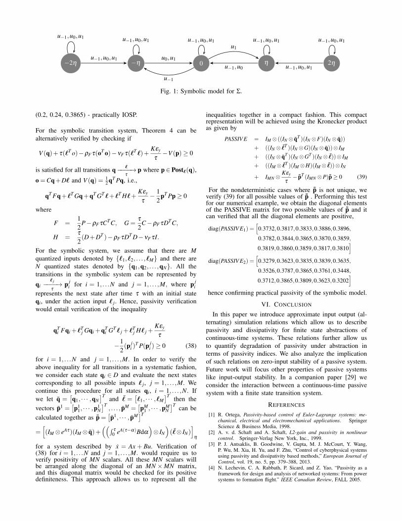
An LTI system Σ : x = −x + u is (0.25,0.5) - IOSP withan output function y = x+u and a storage function V (x) =12 xT (0.5154)x = 0.2577x2. Now we construct a approxi-mately input output similar symbolic model for Σ. It isreadily seen that Σ is incrementally forward complete, thuswe can apply Corollary 1. We work on the subset D =[−0.2,0.2] of state space and subset U = [−0.1,0.1] of theinput space. To construct the symbolic model of precisionεy = 1, we construct a symbolic model Tτ,η ,µ(Σ) by choosingθ1 = 1, η = 0.1, θ2 = εu = µ = 0.1 and τ = 0.2 so thatassumptions of Corollary 1 are satisfied. Since µ = 0.1 andτ = 0.2, the control inputs are piecewise constant of durationτ such that

{−µ,0,µ}= {u−1,u0,u1}= {−0.1,0,0.1} ∈U.

And the states of the symbolic system are described by

{−2η ,−η ,0,η ,2η}= {−0.2,−0.1,0,0.1,0.2} ∈ D.

The transitions between states upon the action of acontrol input can be calculated using the differentialequation describing Σ. The symbolic system in figure1 represents Tτ,η ,µ(Σ) and it can be observed Tτ,η ,µ(Σ)is nondeterministic, i.e., Postu(x) may not be a singleelement. For example, if we consider the state −2η , thePostu0(−2η) = {−2η ,−η}, i.e., under the input u0, thenext possible state may be −2η or −η . In Fig. 1, multipleinputs on the arrows represent all the possible inputs thatcan cause that transition.

Now we discuss the effect of symbolic abstraction on thepassivity properties of Σ. It can be verified that the outputy = x+u satisfies Assumption 1 for γ = 1. Hence Theorem 4states that Tτ,η ,µ(Σ) is

(ρF ,νF ,

Kεyτ

)-practically IOSP where


1+ τ= 0.2583, ρF =

ρ

(1+ τ)τ= 1.0417.

and K is the Lipschitz constant for V (x). For the state spaceD as the Lipschitz constant K = 0.0773, hence Tτ,η ,µ(Σ) is

0 η 2η−η−2ηu−1,u0,u1

u−1,u0,u1 u−1,u0,u1

u0,u1

u−1,u0,u1

u−1

u1

u−1,u0

u−1,u0,u1

u−1,u0,u1

u−1,u0,u1

Fig. 1: Symbolic model for Σ.

(0.2, 0.24, 0.3865) - practically IOSP.

For the symbolic transition system, Theorem 4 can bealternatively verified by checking if

V (q)+ τ(`T o)−ρF τ(oT o)−νF τ(`T `)+Kεy

τ−V (p)≥ 0

is satisfied for all transitions q `−−−−→τ

p where p∈ Post`(q),o =Cq+D` and V (q) = 1

2 qT Pq, i.e.,

qT Fq+`T Gq+qT GT `+`T H`+Kεy

τ− 1

2pT Pp≥ 0

where

F =12

P−ρF τCTC, G =τ

2C−ρF τDTC,

H =τ

2(D+DT )−ρF τDT D−νF τI.

For the symbolic system, we assume that there are Mquantized inputs denoted by {`1,`2, . . . ,`M} and there areN quantized states denoted by {q1,q2, . . . ,qN}. All thetransitions in the symbolic system can be represented by

qi` j−−−−→τ

p ji for i = 1, . . .N and j = 1, . . . ,M, where p j

irepresents the next state after time τ with an initial stateqi, under the action input ` j. Hence, passivity verificationwould entail verification of the inequality

qTi Fqi +`T

j Gqi +qTi GT ` j +`T

j H` j +Kεy

τ

−12(p j

i )T P(p j

i )≥ 0 (38)

for i = 1, . . .N and j = 1, . . . ,M. In order to verify theabove inequality for all transitions in a systematic fashion,we consider each state qi ∈ D and evaluate the next statescorresponding to all possible inputs ` j, j = 1, . . . ,M. Wecontinue this procedure for all states qi, i = 1, . . . ,N. Ifwe let q =

[q1, · · · ,qN

]T and ¯ =[`1, · · · ,`M

]T then thevectors p1 =

[p1

1, · · · ,p1N]T

, . . . , pM =[pM

1 , · · · ,pMN]T can be

calculated together as ¯p =[p1, · · · , pM

]T=[(IM⊗ eAτ)(IM⊗ q)+

((∫τ

0 eA(τ−α)Bdα

)⊗ IN

)( ¯⊗ IN)

]η

for a system described by x = Ax + Bu. Verification of(38) for i = 1, . . .N and j = 1, . . . ,M. would require us toverify positivity of MN scalars. All these MN scalars willbe arranged along the diagonal of an MN ×MN matrix,and this diagonal matrix would be checked for its positivedefiniteness. This approach allows us to represent all the

inequalities together in a compact fashion. This compactrepresentation will be achieved using the Kronecker productas given by

PASSIV E = IM⊗ ((IN ⊗ qT )(IN ⊗F)(IN ⊗ q))+ ((IN ⊗ ¯T )(IN ⊗G)(IN ⊗ q))⊗ IM

+ ((IN ⊗ qT )(IN ⊗GT )(IN ⊗ ¯))⊗ IM

+ ((IM⊗ ¯T )(IM⊗H)(IM⊗ ¯))⊗ IN

+ IMN ⊗Kεy

τ− ¯pT (IMN ⊗P) ¯p≥ 0 (39)

For the nondeterministic cases where ¯p is not unique, weverify (39) for all possible values of ¯p . Performing this testfor our numerical example, we obtain the diagonal elementsof the PASSIVE matrix for two possible values of ¯p and itcan verified that all the diagonal elements are positive,

diag(PASSIV E1) =[0.3732,0.3817,0.3833,0.3886,0.3896,

0.3782,0.3844,0.3865,0.3870,0.3859,

0.3819,0.3860,0.3859,0.3817,0.3810]

diag(PASSIV E2) =[0.3279,0.3623,0.3835,0.3839,0.3635,

0.3526,0.3787,0.3865,0.3761,0.3448,

0.3712,0.3865,0.3809,0.3623,0.3202]

hence confirming practical passivity of the symbolic model.

VI. CONCLUSION

In this paper we introduce approximate input output (al-ternating) simulation relations which allow us to describepassivity and dissipativity for finite state abstractions ofcontinuous-time systems. These relations further allow usto quantify degradation of passivity under abstraction interms of passivity indices. We also analyze the implicationof such relations on zero-input stability of a passive system.Future work will focus other properties of passive systemslike input-output stability. In a companion paper [29] weconsider the interaction between a continuous-time passivesystem with a finite state transition system.

REFERENCES

[1] R. Ortega, Passivity-based control of Euler-Lagrange systems: me-chanical, electrical and electromechanical applications. SpringerScience & Business Media, 1998.

[2] A. v. d. Schaft and A. Schaft, L2-gain and passivity in nonlinearcontrol. Springer-Verlag New York, Inc., 1999.

[3] P. J. Antsaklis, B. Goodwine, V. Gupta, M. J. McCourt, Y. Wang,P. Wu, M. Xia, H. Yu, and F. Zhu, “Control of cyberphysical systemsusing passivity and dissipativity based methods,” European Journal ofControl, vol. 19, no. 5, pp. 379–388, 2013.

[4] N. Lechevin, C. A. Rabbath, P. Sicard, and Z. Yao, “Passivity as aframework for design and analysis of networked systems: From powersystems to formation flight.” IEEE Canadian Review, FALL 2005.

[5] D. S. Laila, D. Nešic, and A. Astolfi, “3 sampled-data control ofnonlinear systems,” in Advanced Topics in Control Systems Theory.Springer, 2006, pp. 91–137.

[6] R. Costa-Castelló and E. Fossas, “On preserving passivity in sampled-data linear systems,” in American Control Conference, 2006. IEEE,2006, pp. 6–pp.

[7] S. Stramigioli, C. Secchi, A. J. Van der Schaft, and C. Fantuzzi, “Sam-pled data systems passivity and discrete port-hamiltonian systems,”Robotics, IEEE Transactions on, vol. 21, no. 4, pp. 574–587, 2005.

[8] F. Zhu, H. Yu, M. J. McCourt, and P. J. Antsaklis, “Passivity and sta-bility of switched systems under quantization,” in Proceedings of the15th ACM international conference on Hybrid Systems: Computationand Control. ACM, 2012, pp. 237–244.

[9] A. Y. Pogromsky, M. Jirstrand, and P. Spangeus, “On stability andpassivity of a class of hybrid systems,” in IEEE Conference onDecision and Control, vol. 4. INSTITUTE OF ELECTRICALENGINEERS INC (IEE), 1998, pp. 3705–3710.

[10] M. Zefran, F. Bullo, and M. Stein, “A notion of passivity for hybridsystems,” in Decision and Control, 2001. Proceedings of the 40th IEEEConference on, vol. 1. IEEE, 2001, pp. 768–773.

[11] J. Zhao and D. J. Hill, “Dissipativity theory for switched systems,”Automatic Control, IEEE Transactions on, vol. 53, no. 4, pp. 941–953, 2008.

[12] M. K. Çamlıbel, W. Heemels, and J. Schumacher, “On linear passivecomplementarity systems,” European Journal of Control, vol. 8, no. 3,pp. 220–237, 2002.

[13] A. Bemporad, G. Bianchini, and F. Brogi, “Passivity analysis andpassification of discrete-time hybrid systems,” Automatic Control,IEEE Transactions on, vol. 53, no. 4, pp. 1004–1009, 2008.

[14] J. E. Cury, B. H. Krogh, and T. Niinomi, “Synthesis of supervisorycontrollers for hybrid systems based on approximating automata,”Automatic Control, IEEE Transactions on, vol. 43, no. 4, pp. 564–568, 1998.

[15] J. A. Stiver, X. D. Koutsoukos, and P. J. Antsaklis, “An invariant-based approach to the design of hybrid control systems,” InternationalJournal of Robust and Nonlinear Control, vol. 11, no. 5, pp. 453–478,2001.

[16] T. Moor, J. Raisch, and S. O’Young, “Discrete supervisory control ofhybrid systems based on l-complete approximations,” Discrete EventDynamic Systems, vol. 12, no. 1, pp. 83–107, 2002.

[17] D. C. Tarraf, A. Megretski, and M. A. Dahleh, “A framework forrobust stability of systems over finite alphabets,” Automatic Control,IEEE Transactions on, vol. 53, no. 5, pp. 1133–1146, 2008.

[18] K. M. Passino, A. N. Michel, and P. J. Antsaklis, “Lyapunov stabilityof a class of discrete event systems,” Automatic Control, IEEETransactions on, vol. 39, no. 2, pp. 269–279, 1994.

[19] A. Girard, G. J. Pappas et al., “Approximation metrics for discreteand continuous systems,” Automatic Control, IEEE Transactions on,vol. 52, no. 5, pp. 782–798, 2007.

[20] M. Zamani, G. Pola, M. Mazo, and P. Tabuada, “Symbolic models fornonlinear control systems without stability assumptions,” AutomaticControl, IEEE Transactions on, vol. 57, no. 7, pp. 1804–1809, 2012.

[21] P. Tabuada, Verification and control of hybrid systems: a symbolicapproach. Springer, 2009.

[22] P. Tabuada and G. J. Pappas, “Linear time logic control of discrete-timelinear systems,” Automatic Control, IEEE Transactions on, vol. 51,no. 12, pp. 1862–1877, 2006.

[23] Y. Tazaki and J.-i. Imura, “Finite abstractions of discrete-time linearsystems and its application to optimal control,” in 17th IFAC worldcongress, 2008, pp. 10 201–10 206.

[24] Y. Sun, H. Lin, and B. M. Chen, “An input–output simulationapproach to controlling multi-affine systems for linear temporal logicspecifications,” International Journal of Control, vol. 85, no. 10, pp.1464–1476, 2012.

[25] H. K. Khalil and J. Grizzle, Nonlinear systems. Prentice hall UpperSaddle River, 2002, vol. 3.

[26] Z.-P. Jiang and Y. Wang, “Input-to-state stability for discrete-timenonlinear systems,” Automatica, vol. 37, no. 6, pp. 857–869, 2001.

[27] Y. Oishi, “Passivity degradation under the discretization with the zero-order hold and the ideal sampler,” in Decision and Control (CDC),2010 49th IEEE Conference on. IEEE, 2010, pp. 7613–7617.

[28] Z.-P. Jiang and Y. Wang, “A converse lyapunov theorem for discrete-time systems with disturbances,” Systems & control letters, vol. 45,no. 1, pp. 49–58, 2002.

[29] S. Sajja, V. Gupta and P. Antsaklis “On passivity of a con-tinuous plant interconnected with a discrete supervisory con-troller,” Submitted for Publication in CDC 2015, Technical reportavailable at (http://www3.nd.edu/~isis/techreports/isis-2014-005.pdf).

[30] X. Xu, N. Ozay, V. Gupta “Dissipativity degradation in discrete controlimplementations: an approximate bisimulation approach,” Submittedfor Publication in CDC 2015.

On passivity of a continuous plant interconnected with a discretesupervisory controller

Shravan Sajja1∗, Vijay Gupta2 and Panos J. Antsaklis2

Abstract— Consider a continuous plant interconnected witha discrete supervisory controller. In what sense can the in-terconnection be termed passive and stable? This question isuseful for application of passivity based control techniques incyberphysical systems where controllers may be implementedin software. Using a notion of passivity for a finite state modelabstracted from an infinite state continuous system that wasproposed in [13], hence we consider the interaction of suchfinite state models of a plant with discrete controllers. Thechief result of this paper is to find conditions that ensure thatthe entire interconnection is passive and hence stable.

I. INTRODUCTION

Close interaction between dynamic systems and thecomputational elements in a cyberphysical systemmakes it desirable that these computational elementsare designed while exploiting the properties (for e.g.passivity, dissipativity, symmetry, invariance, etc.) of adynamic system. In this paper, we are primarily interestedin the interaction between computational elements andpassive dynamic systems. Passivity is an important propertyused to design stable control systems that also offerscompositionality [1]. Hence, there is much interest in usingpassivity as design tool for cyberphysical systems [2].For a full theory of passivity in cyberphysical systemswe need a better understanding of the interaction betweenpassive dynamic systems with computational elements thatare discrete state systems. However, this needs a welldefined notion of passivity for discrete state systems. Onebroad approach to solve this problem has been throughthe hybrid systems framework. Hybrid system considerboth continuous and discrete dynamics are considered inthe same framework and several definitions of passivityhave proposed for certain special classes of hybrid systems[3], [4], [5], [6], [7]. Although hybrid systems frameworkis well established, systematic compositional methods toanalyze the interconnection between discrete controllersand continuous plants are not yet available. We follow analternate approach based on abstracting finite state modelsfrom infinite state models (continuous-time systems) whichfurther interact with computational elements modeled usingfinite state controllers (see figure 1). This approach providesus with a unified framework to analyze both discrete and

*This work was done when author was in Department of ElectricalEngineering, University of Notre Dame, Notre Dame, IN 46556, USA

1 Author is with IBM Research Dublin, [email protected]

2 Authors are with the Department of Electrical Engineering,University of Notre Dame, Notre Dame, IN 46556, [email protected], [email protected]

continuous components of a cyberphysical system. In [13]we showed that if the finite state transition systems areabstracted using the concepts of approximate input outputsimulation relationships then properties like passivity anddissipativity can be defined for the finite state abstractions.Further, we quantified the degradation of passivity undersuch abstractions and showed that finite abstractions of acertain class of continuous-time passive systems are zeroinput asymptotically stable in a practical sense.

In this paper we present results on passivity for systemsobtained by composing of such practically passive finite stateabstractions. Specifically, we analyze feedback compositionof computational elements with finite abstractions ofcontinuous-time passive systems. We adopt a modifiednotion of approximate feedback composition of transitionsystems proposed by [10], which requires two transitionsystems to satisfy certain approximate simulation relationsfor feedback composition. We show that once two transitionsystems are approximately feedback composable, thenpractical passivity of one of those transition systems impliespractical passivity of entire composition, although thepassivity indices may be different. We also show that theseresults can be used to develop practically passivating discretecontrollers for the interconnection of a continuous-timesystems and the discrete controller. However, actual designof such controllers in out of the scope of this paper. Amajor assumption in our work is that both continuous anddiscrete components of the cyberphyiscal system receive thesame quantized inputs and is the subject of our future work.

This paper is organized as follows. In section II of this paperwe introduce our notation and some preliminary definitions.In section III, we present some initial results for feedbackcomposition of finite transition systems. We further interpretthese results for the case when a discrete supervisor isconnected to a continuous-time passive system. We show thatif one of the components in the interconnection is passivethen their approximate feedback composition is also passivein a practical sense. We would also like to mention the paper[14] that considers the related but complementary problemof discretizing a controller designed in the continuous spaceso that passivity indices of the closed loop system are main-tained despite discretization. Note that while [14] requires abisimulation of the controller, we require a simulation of theplant for our purpose.

Discrete to continuous Continuous to discrete

Measurement

Symbol Symbol

Control inputPhysical System

Software

Discrete abstraction

Fig. 1: Finite state approximation of a continuous-time plantinteracting with a finite state controllers (software).

II. PRELIMINARIES

A. Notation

The identity map on a set A is denoted by 1A. If A isa subset of B we denote by ıA : A ↪→ B or simply byı the natural inclusion map taking any a ∈ A to ı(a) =a ∈ B. The symbols N, Z, R, R+ and R+

0 denote theset of natural, integer, real, positive, and nonnegative realnumbers, respectively. The inner product of signals u(t), y(t)is denoted by 〈u,y〉 defined as 〈u,y〉=

∫ t0 uT (τ)y(τ)dτ . Given

a vector x ∈ Rn, xi is the i-th element of x and we denoteinfinity norm and euclidean norms of x by ‖x‖ and ‖x‖2.Given a measurable function f : R+ : 0← Rn the (essential)supremum (sup norm) of f is denoted by ‖‖∞. If A⊆Rn andη ∈R+, [A]η denotes the subset [A]η ⊆ A defined by: [A]η ={

z ∈ A | zi = kiη for some ki ∈ A and i = 1,2, . . . ,n}. The

set [A]η will be used as an approximation of the set Awith precision η . If we define Bε(x) = {y ∈ Rn| ‖x− y‖ ≤ε}. For set A ⊆ Rn of the form A =

⋃Mj=1 A j for some

M ∈ N, where A j = Πni=1[c

ji ,d

ji ] ⊆ Rn with c j

i < d ji and

positive constant η ≤ η , where η = min j=1,...,M ηA j andηA j = min{|d j

1− c j1|, · · · , |d

jn− c j

n|}. Note that [A]η 6= ∅ forany η ≤ η . Geometrically, for any η ∈ R+ and λ ≥ η thecollection of sets {Bλ (p)}p∈[A]η is a covering of A, i.e. A⊆⋃

p∈[A]η Bλ (p). A continuous function γ : R+0 → R+

0 belongsto class K if it is strictly increasing and γ(0) = 0; γ belongsto class K∞ if γ ∈K and γ(r)→∞ as r→∞. A continuousfunction γ : R+

0 ×R+0 → R+

0 belongs to class K L if, foreach fixed s, the map β (r,s) belongs to class K∞ with respectto r and, for each fixed r, the map β (r,s) is decreasing withrespect to s and β (r,s)→ 0 as s→ ∞. A relation R⊆ A×Bis defined by a map of the form R : A→ 2B where b∈ R(a) ifand only if (a,b) ∈ R. For a set S ∈ A the set R(S) is definedas R(S) = {b∈ B : ∃ a∈ S,(a,b)∈ R}. Also, R−1 denotes theinverse relation defined by R−1 = {(b,a)∈B×A : (a,b)∈R}.We also denote by d : X ×X → R+

0 a metric in the space Xand by πX : X×U→ X the projection sending (x,u)∈ X×Uto x ∈ X .

B. Incremental forwardness and stability

In this work we restrict ourselves to control systems of theform

Σ = (Rn,U,U , f ) (1)

where• Rn is the state space;• U⊆ Rm is the input space;• U :R→U is a subset of the set of all locally essentially

bounded functions of time from intervals of the form]a,b[⊆ R to U with a < 0 and b > 0;

• f : Rn×U→ Rn is a Lipschitz continuous map.If ξ :]a,b[−−→ Rn is a trajectory of Σ (or equivalently asolution of the differential equation x = f (x,u)), then wewill use ξ (τ,x,v) to denote a unique point reached at timeτ under the input v from an initial condition x. System Σ issaid to be forward-complete if such a solution is defined forall t ∈]0,∞[. In this paper we use an incremental version ofthis property, defined as:

Definition 1 (Incremental forward-completeness): Acontrol system Σ is δ -FC if there exist continuous functionsβ : R+

0 ×R+0 → R+

0 and γ : R+0 ×R+

0 → R+0 such that for

every s∈R+, the functions β (·,s) and γ(·,s) belong to classK∞, and for any x,x′ ∈ Rn, any τ ∈ R+, and any v,v′ ∈U ,where v,v′ : [0,τ)→ U, the following condition is satisfiedfor all t ∈ [0,τ]:

‖ξ (t,x,v)−ξ (t,x′,v′)‖ ≤ β (‖x− x′‖, t)+ γ(‖v− v′‖∞, t).(2)

C. Transition systems and system relations

Definition 2: [10] A system Tq is a quintuple Tq =

(Q,L, `−−−−→τ

,O,H) consisting of:

• a finite set of states q ∈ Q;• a finite set of inputs ` ∈ L;• a transition relation −−→⊆ Q×L×{τ}×Q;• an output set O;• an output function H : Q→ O.

Tq can be thought of as a discrete time system with a sampletime τ and a finite state run

q0`0−−−−→τ

q1`1−−−−→τ

q2`2−−−−→τ· · · `n−2−−−→ qn−1

`n−1−−−−→τ

qn

where q0 ∈ Q is the initial state and qi`i−−−−→τ

qi+1 for all0≤ i≤ n. The subscript i corresponds to the sampling timeinstants t = 0,1,2, . . . ,nτ and qi corresponds to the stateof Tq at the time instant iτ . In some cases, a finite staterun can be extended to an infinite state run with i ∈ N. Todefine notions of stability for transition systems we assumethat the finite sets Q,L, and O are equipped with the metricgiven by d(p,q) = ‖p−q‖ where p,q are elements of Q,Lor O. Tq is deterministic, if for any state q ∈ Q and ` ∈ Lthere exists at most one state q′ ∈ Q such that q `−−−→ q′;if the system is nondeterministic, then for a transitionq `−−−→ q′ the state q′ may not unique, q′ is also known as

the `-successor of q. In such a case q′ belongs to a set ofall possible `-successors given by Post`(q) and we will useL(q) to denote the set of inputs ` ∈ L for which Post`(q) isnonempty. We will further use Post`(Q) to denote the set⋃

q∈Q Post`(q). Now we present certain system relations,that are used in this paper.

Definition 3: [11](ε-Approximate Simulation and Alter-nating Simulation) Let T1 := (Q1,L1,−−−−→

1,O1,H1), T2 :=

(Q2,L2,−−−−→2

,O2,H2) be metric transition systems with thesame sets of inputs L= L1 = L2 and outputs O=O1 =O2 andequipped with the metric d. Let ε ∈ R+

0 be given precisionrequirements then a relation R⊆ Q1×Q2 is said to be an(a) an ε-approximate Simulation (ε-S) relation between T1

and T2 if the following two conditions are satisfied:(i) for every (q1,q2)∈R we have d(H1(q1),H2(q2))≤

ε;(ii) for every (q1,q2) ∈ R we have that q1

`1−−−−→1

q′1

in T1 implies the existence of q2`2−−−−→2

q′2 in T2

satisfying (q′1,q′2) ∈ R.

(b) an ε-approximate Alternating Simulation (ε-AS) rela-tion from T1 to T2 if conditions (i), (ii) and the followingcondition are satisfied:(iii) for every (q1;q2) ∈ R and for every `1 ∈ L1(q1)

there exists `2 ∈ L2(q2) such that for every q′2 ∈Post`2(q2) there exists q′1 ∈ Post`1(q1) satisfying(q′2,q

′1) ∈ R.

If T1 is ε- approximately simulated (or alternatingly simu-lated) by T2, then we denote this fact by T1�ε

S T2 (T1�εAS T2).

Approximate simulation relations used in [11], are primarilybased on bounding the distance between the outputs or statesof the continuous-time and its approximation. However, inorder to account for behaviors like passivity (which aredefined using both inputs and outputs) we introduced notionsof approximate input output simulation and approximateinput output alternating simulation. These notions allow usto bound the distances between outputs as well as inputs. Ifεu and εy are the given precision requirements for inputs andoutputs respectively and if T1 is (εu,εy)- approximately inputoutput simulated (or approximately input output alternatinglysimulated) by T2, then we denote this fact by T1 �

(εu,εy)IOS T2(

T1 �(εu,εy)IOAS T2

).

Definition 4 (Approximate input output simulation):Let T1 := (X1,U1,−−−−→

1,Y1,H1), T2 := (X2,U2,−−−−→

2,Y2,H2) be metric transition systems with the same sets ofinputs U = U1 = U2 and outputs Y = Y1 = Y2 and equippedwith the metric d. Let εu,εy ∈ R+

0 be given precisionrequirements then a relation R ⊆ X1×X2 is said to be an(εu,εy) - approximate input output simulation (IOS) relationbetween T1 and T2 if the following two conditions aresatisfied:(i) for every (x1,x2) ∈ R we have d(H1(x1),H2(x2))≤ εy;

(ii) for every (x1,x2) ∈ R and for every u1 ∈U1 there existsu2 ∈U2 such that d(u1,u2)≤ εu and x1

u1−−−−→1

x′1 in T1

implies the existence of x2u2−−−−→2

x′2 in T2 such that

(x′1,x′2) ∈ R.

Definition 5: (Approximate input output alternatingsimulation): Let T1 := (X1,U1,−−−−→

1,Y1,H1), T2 :=

(X2,U2,−−−−→2

,Y2,H2) be metric transition systems with thesame sets of inputs U = U1 = U2 and outputs Y = Y1 = Y2and equipped with the metric d. Let εu,εy ∈ R+

0 be a givenprecision requirements, a relation R ⊆ X1×X2 is said to bean (εu,εy) - approximate input output alternating simulation(IOAS) relation from T1 to T2 if condition (i) of Definition4 and the following condition are satisfied:(iii) for every (x1,x2) ∈ R and for every u1 ∈U1(x1) there

exists u2 ∈U2(x2) such that d(u1,u2)≤ εu and for everyx′2 ∈ Postu2(x2) there exists x′1 ∈ Postu1(x1) satisfying(x′2,x

′1) ∈ R.

The two notions of alternating approximate simulation andapproximate simulation coincide in the special case of de-terministic systems. If T1 is (εu,εy)- approximately inputoutput simulated (or approximately input output alternatinglysimulated) by T2, then we denote this fact by T1 �

(εu,εy)IOS T2

(T1 �(εu,εy)IOAS T2). In this paper, we use a special case of

approximate input-output simulation described in [13]. Thisspecial case is obtained when we set εu = 0 and such a casearises when both transition systems T1 and T2 are connectedto the same input signal.

Definition 6: ((0,εy)-Approximate input outputsimulation) Let T1 := (Q1,L1,−−−−→

1,O1,H1),

T2 := (Q2,L2,−−−−→2

,O2,H2) be metric transition systemswith the same sets of inputs L = L1 = L2 and outputsO = O1 = O2 and equipped with the metric d. Let εy ∈ R+

0be given precision requirement for the outputs, then arelation R⊆ Q1×Q2 is said to be(a) an (0,εy) - approximate input output simulation (IOS)

relation between T1 and T2 if the following two condi-tions are satisfied:(i) for every (q1,q2)∈R we have d(H1(q1),H2(q2))≤

εy;(ii) for all ` ∈ L and for every (q1,q2) ∈ R we have

that q1`−−−−→1

q′1 in T1 implies the existence of

q2`−−−−→2

q′2 in T2 satisfying (q′1,q′2) ∈ R.

(b) an (0,εy) - approximate input output alternating simu-lation (IOAS) relation between T1 and T2 if conditions(i), (ii) and the following condition is satisfied:(iii) for every (q1;q2) ∈ R, L1(q1) = L2(q2) = L and

for every ` ∈ L and for every q′2 ∈ Post`(q2) thereexists q′1 ∈ Post`(q1) satisfying (q′2,q

′1) ∈ R.

Proposition 1: Consider two transitions systems T1 andT2 such that both transition systems receive the same inputsignal. Then (0,εy) - approximate input output (alternating)simulation and ε-approximate (alternating) simulation (fromdefinition 3) are equivalent.PROOF: The proof follows from Definition 3 by setting `1 =`2.

�

D. Finite abstractions

In order to a obtain finite abstraction for Σ = (Rn,U,U , f ),we begin by considering a discrete time sub-transition systemTτ(Σ) with a sampling time period τ ∈ R+. We furtherassume that control inputs are piecewise-constant over thesampling time period τ , the class of inputs considered are:

Uτ := {u ∈U | u(t) = u(0), t ∈ [0,τ]}.

For Tτ(Σ) we use identity map as the output function,however, for stability and passivity analysis, we use analternate output corresponding to y = h(x,u).

Definition 7: [10] Let Σ be a control system and T (Σ) itsassociated transition system. For any τ > 0, the sub transitionsystem Tτ(Σ) := (Xτ ,Uτ ,

uτ−−−−→τ

,Yτ ,Hτ) is defined by:

• Xτ = Rn;• Uτ = Uτ ;• xτ

uτ−−−−→τ

x′τ , if there exists a trajectory ξ : [0,τ]−−−→ξ (τ,xτ ,uτ) = x′τ ;

• Yτ = Rn;• Hτ = 1Rn .

Now we restrict the input set to a hyper-rectanlge U ⊆ Rm

such that {0} ∈ U. Then we choose the input quantizationfactor such that µ ≤ µ (see A. Notation on how to calculateµ). Now we consider the transition system Tτ(Σ) with aquantized input space to obtain Tτ,µ(Σ) defined as:

Tτ,µ(Σ) := (Xτ ,Uq,uq−−−→,Yτ ,Hτ)

where• Xτ = Rn;• Uq = [U]µ ;• xτ

uq−−−−→τ

x′τ , if there exists a trajectory ξ : [0,τ]−−−→ξ (τ,xτ ,uq) = x′τ ;

• Yτ = Rn;• Hτ = 1Rn .

In this final stage, we restrict the state set to a hyper-rectanlge X ⊆ Rn such that {0} ∈ X . Then we choose thestate quantization factor such that η ≤ η (see A. Notationon how to calculate η). Then for any δ -FC control system Σ

and parameters τ > 0, η > 0, µ > 0 and a design parametersθ1,θ2 ∈R+, a countable transition system [9] can be definedas:

Tτ,µ,η(Σ) := (Xq,Uq,uq−−−−→τ

,Yq,Hq) (3)

where:• Xq = [X ]η ;• Uq = [U]µ ;• xq

uq−−−−→τ

x′q, if ‖ξ (τ,xq,uq) − x′q‖ ≤ β (θ1,τ) +

γ(θ2,τ)+η ;• Yq = [X ]η• Hq = ı : Xq ↪→ Yq

where β and γ are functions from Definition 1. Thetransition system Tτ,µ,η(Σ) is finite and countable [9]. A

slight modification of Theorem 4.1 from [9] can be usedto obtain finite countable abstractions Tτ,η ,µ(Σ) which are(0,εy) - approximately input output alternatingly similar toTτ,µ(Σ) and hence we can state the following result.

Proposition 2: [13] Consider a control system Σ and anydesired precision εu = 0, εy > 0. If Σ is δ -FC then for any τ >0, θ > 0, η > 0 and µ > 0 satisfying the following inequality:

β (θ1,τ)+ γ(θ2,τ)+η ≤ εy, (4)

such that η ≤ εy ≤ θ1 and µ ≤ θ2, we have:

Tτ,η ,µ(Σ)�(0,εy)IOAS Tτ,µ(Σ)�

(0,εy)IOS Tτ,η ,µ(Σ). (5)

PROOF: To show Tτ,µ(Σ) �(0,εy)IOS Tτ,η ,µ(Σ) we consider any

xτ ∈ Xτ and any uq ∈Uq = [U]µ , then there exists xq ∈ Xq =[X ]η such that

‖xτ − xq‖ ≤ η ≤ εy (6)

hence condition (i) of Definition 6 is satisfied.

Now if we consider the transition xτ

uq−−−−→τ

x′τ in thetransition system Tτ,µ(Σ) , then the distance between x′τ andξ (τ,xq,uq) can estimated based on the δ - FC property ofΣ and inequality (6) i.e.,

‖x′τ −ξ (τ,xq,uq)‖ ≤ β (εy,τ)+ γ(0,τ) (7)

Since Xτ ⊆⋃

p∈[X ]η Bλ (p), there exists x′q ∈ Xq such that

‖x′τ − x′q‖ ≤ η (8)

From the triangular inequality we have

‖ξ (τ,xq,uq)− x′q‖ ≤ ‖ξ (τ,xq,uq)− x′τ‖+‖x′τ − x′q‖


‖ξ (τ,xq,uq)− x′q‖ ≤ β (εy,τ)+ γ(0,τ)+η

Finally we use η ≤ εy ≤ θ1 and 0 < θ2 to show that



uq−−−→ x′q in Tτ,µ,η(Σ). Therefore, from inequality (8)and since η ≤ εy we conclude that (x′τ ,x

′q)∈ R and condition

(ii) in Definition 6 holds.

Now we show that Tτ,η ,µ(Σ) �(0,εy)IOAS Tτ,µ(Σ). For R ⊆ Xτ ×

Xq we consider an xτ = xq ∈ Xq. This is possible becauseXq ⊆ Xτ and it satisfies condition (i) of Definition 4 (i.e.,‖xτ − xq‖ = 0 < εy). Now we choose an input uq ∈Uq andconsider the unique transition xτ

uq−−−−→τ

x′τ = ξ (τ,xτ ,uq) ∈Postuq(xτ). The distance between x′τ and ξ (τ,xq,uq) can bebounded using the δ - FC properties of Σ, i.e.,

‖x′τ −ξ (τ,xq,uq)‖ ≤ β (0,τ)+ γ(0,τ) (9)

Since Xτ ⊆⋃

p∈[X ]η Bλ (p), we can always find x′q ∈ Xq suchthat

‖x′q− x′τ‖ ≤ η (10)

From the triangular inequality and inequalities (9) and (10)we have

‖ξ (τ,xq,uq)− x′q‖ ≤ ‖ξ (τ,xq,uq)− x′τ‖+‖x′τ − x′q‖≤ β (0,τ)+ γ(0,τ)+η

Finally we use 0 < θ1 and 0 < θ2 to show that




′q) ∈ R and

condition (iii) in Definition 6 holds.

�

Finitely abstracted transition system (3) is a quantized ver-sion of the sampled-data system Tτ(Σ). The finite statetransition system (3) can be thought of as a discrete timesystem with a finite state run

xq0

uq0−−−−→τ

xq1

uq1−−−−→τ

xq2

uq2−−−−→τ· · ·

uq(n−2)−−−−→ xqn−1

uq(n−1)−−−−→τ

xqn

where xq0 ∈ Xq is the initial state and xqiuqi−−−−→τ

xq(i+1) forall 0 ≤ i ≤ n. The subscript i corresponds to the samplingtime instants t = 0,1τ,2τ, . . . ,nτ and xqi corresponds to thestate of (3) at the time instant iτ .

E. Dissipativity and passivity

Consider the system Σ and an output function y = h(x,u) ∈Rp. Further, assume that f (0,0) = 0 and h(0,0) = 0. Σ isdissipative w.r.t. y = h(x,u) if there exists a C 1 storagefunction V (x) : Rn→R+

0 and a supply rate ω : U×Rp→R+0

such that V (0) = 0 and the following inequality is satisfied:

V (x(t2))−V (x(t1))≤∫ t2

t1ω(u,y,x)dt (11)

for any t2 ≥ t1 and u ∈U . A special case of dissipativity is(ρ,ν) - input output strict passivity (IOSP) when ω(u,y,x)=uT y−νuT u−ρyT y with ρ,ν ∈R+

0 . In this definition, param-eters ν and ρ are known as passivity indices. Correspondingto continuous-time notions of dissipativity and passivity, weintroduced the notions of practical dissipativity and practicalpassivity for transition systems in [13].

Definition 8 (Practical dissipativity): Let C 1 function V :Xq → R+

0 be a storage function with V (0) = 0 and let ω :Uq×Xq→R be a supply rate, then the transition system (3)is practically dissipative with respect to ω if

1τ

(V (xq(i+1))−V (xqi)

)≤ω(uqi,xqi)+δ ∀i∈N and δ > 0

(12)for all the transitions xqi


xq(i+1).

The transition system (3) is (ρF ,νF ,δ )-practically IOSPwhen the supply rate is ω(uqi,xqi) = (uT

qih(xqi,uqi)) −

ρF(hT (xqi,uqi)h(xqi,uqi))− νF(uTqiuqi). The function yi =

h(xqi,uqi) is an output function for the finite transition systemat a time instant iτ and it is analogous to y = h(x,u) forthe continuous-time system. Note that this output functionis different from the output function Hq = ı : Xq ↪→ Yq. Theoutput function yi = h(xqi,uqi) will be used only to studypassivity and the stability behavior of the transition system.In order to avoid confusion between the output functionsHq and yi = h(xqi,uqi), we will refer to yi = h(xqi,uqi) asthe passive output function, i.e., the output with respect towhich the system is passive. The passive output functionfor a transition system can be obtained using Hq = ı : Xq ↪→Yq, whenever Hq = 1Xq , i.e., y = h(Hq(xq),uq) = h(xq,uq).An important consequence of practical IOSP is practicalasymptotic stability.

Corollary 1: The transition system (3) is practicallyasymptotically stable for zero input (uqi ≡ 0) if there existsclass K∞ functions α , α , θ such that for any strictly positivereal numbers ∆,δ and for all xq ∈ Xq such that ‖xq‖ ≤ ∆, thefollowing holds

α(‖xq‖)≤V (xq)≤ α(‖xq‖), (13)θ(‖xq‖)≥ ρF τhT (xq,0)h(xq,0), (14)

θ(α−1 ◦α(∆))> δ (15)

and (3) is (ρF ,νF ,δ )-practically IOSP with ρF > 0 and νF ≥0.Now we present a result which quantifies the degradation ofpassivity under finite state approximations which are approx-imately input output similar to continuous-time systems. Thisresult was presented in [13] and it is based on an assumptionfrom [12].

Theorem 1: [13] Suppose that the original continuous-time system Σ is δ - FC and (ν , ρ) - IOSP w.r.t. the passiveoutput function y = h(x,u) and a storage function V with aLipschitz constant K. We also assume that the operator fromu(t) to y(t) has the finite L2 gain, γ , that is∫

τ

0‖y(t)‖2

2dt ≤ γ2∫

τ

0‖u(t)‖2

2dt

for any τ ≥ 0 and admissible u(t). Let Tτ(Σ) be the transitionsystem corresponding to Σ with a sampling time τ . If thestate and input quantization parameters η and µ are chosensuch that Tτ,µ,η(Σ) is (εu,εy) - approximately input outputsimilar (or alternatingly similar) to Tτ(Σ), then Tτ,µ,η(Σ) is(

ρF ,νF ,Kεy

τ

)-practically IOSP w.r.t. to the passive output

function yq = h(xq,uq) and


1+ τρF =

ρ

(1+ τ)τ.

In the next section we consider the problem of feedbackcomposition of a discrete controller Tq and the finite stateabstraction of continuous-time IOSP system Σ given byTτ,µ,η(Σ). Discrete controllers Tq are designed for continuousplants to satisfy certain discrete and/or continuous specifica-tions, for example, discrete supervisory controllers are usedfor mode selection, trajectory planning etc. In the section,

our main goal is analyze the extra conditions imposed onTq and on the nature of feedback composition such that theinterconnection of Tq and Tτ,µ,η(Σ) is also practically IOSPand hence practically asymptotically stable.

III. COMPOSITION OF TRANSITION SYSTEMS

We begin this section by presenting a modified notionof approximate feedback composition of transition systemsfrom [10]. In Sub-section III-B we consider the approxi-mate feedback composition of two transition systems whereone of them is practically IOSP. We show that once twotransition systems are approximately feedback composable,then practical passivity of one of those transition systemsimplies practical passivity of entire composition, althoughwith different passivity indices. Thus, guaranteeing practicalstability for the composed transition system. In Sub-sectionIII-C we show that these results have the potential to developpassivating discrete controllers for continuous-time systems.

A. Feedback composition

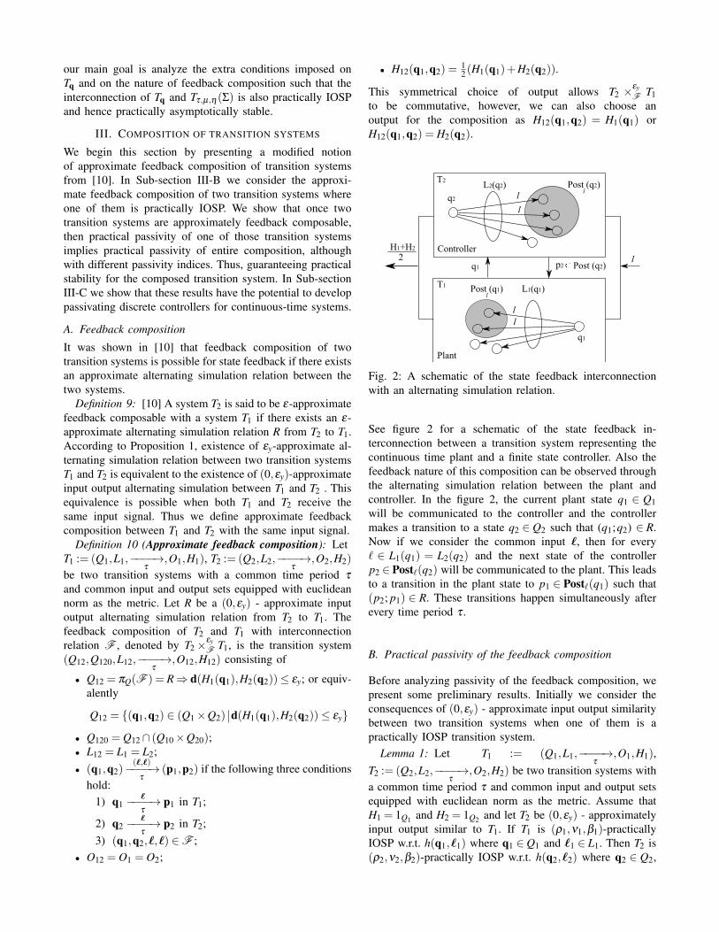
It was shown in [10] that feedback composition of twotransition systems is possible for state feedback if there existsan approximate alternating simulation relation between thetwo systems.

Definition 9: [10] A system T2 is said to be ε-approximatefeedback composable with a system T1 if there exists an ε-approximate alternating simulation relation R from T2 to T1.According to Proposition 1, existence of εy-approximate al-ternating simulation relation between two transition systemsT1 and T2 is equivalent to the existence of (0,εy)-approximateinput output alternating simulation between T1 and T2 . Thisequivalence is possible when both T1 and T2 receive thesame input signal. Thus we define approximate feedbackcomposition between T1 and T2 with the same input signal.

Definition 10 (Approximate feedback composition): LetT1 := (Q1,L1,−−−−→

τ,O1,H1), T2 := (Q2,L2,−−−−→

τ,O2,H2)

be two transition systems with a common time period τ

and common input and output sets equipped with euclideannorm as the metric. Let R be a (0,εy) - approximate inputoutput alternating simulation relation from T2 to T1. Thefeedback composition of T2 and T1 with interconnectionrelation F , denoted by T2×

εyF T1, is the transition system

(Q12,Q120,L12,−−−−→τ

,O12,H12) consisting of

• Q12 = πQ(F ) = R⇒ d(H1(q1),H2(q2))≤ εy; or equiv-alently

Q12 = {(q1,q2) ∈ (Q1×Q2) d(H1(q1),H2(q2))≤ εy}

• Q120 = Q12∩ (Q10×Q20);• L12 = L1 = L2;• (q1,q2)

(`,`)−−−−→τ

(p1,p2) if the following three conditionshold:

1) q1`−−−−→τ

p1 in T1;

2) q2`−−−−→τ

p2 in T2;3) (q1,q2,`,`) ∈F ;

• O12 = O1 = O2;

• H12(q1,q2) =12 (H1(q1)+H2(q2)).

This symmetrical choice of output allows T2 ×εyF T1

to be commutative, however, we can also choose anoutput for the composition as H12(q1,q2) = H1(q1) orH12(q1,q2) = H2(q2).

q1

Post (q1)

L2(q2)

l

l

l

q2 l

l

Post (q2)l

T1

T2

L1(q1)

Controller

Plant

q1 p2 Post (q2)l

H1+H2

2

Fig. 2: A schematic of the state feedback interconnectionwith an alternating simulation relation.

See figure 2 for a schematic of the state feedback in-terconnection between a transition system representing thecontinuous time plant and a finite state controller. Also thefeedback nature of this composition can be observed throughthe alternating simulation relation between the plant andcontroller. In the figure 2, the current plant state q1 ∈ Q1will be communicated to the controller and the controllermakes a transition to a state q2 ∈ Q2 such that (q1;q2) ∈ R.Now if we consider the common input `, then for every` ∈ L1(q1) = L2(q2) and the next state of the controllerp2 ∈ Post`(q2) will be communicated to the plant. This leadsto a transition in the plant state to p1 ∈ Post`(q1) such that(p2; p1) ∈ R. These transitions happen simultaneously afterevery time period τ .

B. Practical passivity of the feedback composition

Before analyzing passivity of the feedback composition, wepresent some preliminary results. Initially we consider theconsequences of (0,εy) - approximate input output similaritybetween two transition systems when one of them is apractically IOSP transition system.

Lemma 1: Let T1 := (Q1,L1,−−−−→τ

,O1,H1),T2 := (Q2,L2,−−−−→

τ,O2,H2) be two transition systems with

a common time period τ and common input and output setsequipped with euclidean norm as the metric. Assume thatH1 = 1Q1 and H2 = 1Q2 and let T2 be (0,εy) - approximatelyinput output similar to T1. If T1 is (ρ1,ν1,β1)-practicallyIOSP w.r.t. h(q1,`1) where q1 ∈Q1 and `1 ∈ L1. Then T2 is(ρ2,ν2,β2)-practically IOSP w.r.t. h(q2,`2) where q2 ∈ Q2,

`1 = `2 = ` ∈ L = L1 = L2 and

ρ2 = ρ1 (1−α2)

ν2 =(

ν1−α1

2

)(16)

β2 =1

2α1M2

ε2y +ρ1

(1

α2+1)

M2ε

2y +β1 +

2Kεy

τ

where K and M are Lipschitz constants of the storagefunction V and the passive output function h(q,`), i.e., forany p,q ∈ Q1∪Q2 and an arbitrary ` ∈ L we have |V (p)−V (q)| ≤ K‖p−q‖ and ‖h(p,`)−h(q,`)‖2 ≤M‖p−q‖ andα1 and α2 ∈ R+ are such that

ν1−α1

2≥ 0 and 1−α2 ≥ 0.

PROOF: Consider (q1,q2)∈ R and an input `∈ L = L1(q1) =L2(q2), then for every p2 ∈ Post`(q2), we have p1 ∈Post`(q1) such that ‖p1−p2‖ ≤ εy. Since T1 is (β1,ρ1,ν1)-IOSP w.r.t. to the passive output function h(q,`), for anytransition q1

`−−−−→τ

p1 in T1 we have

V (p1)−V (q1) ≤ (`T h(q1,`))τ−ρ1(hT (q1,`)h(q1,`))τ

−ν1(`T `)τ +β1τ (17)

Also from the Lipschitz continuity of the storage functionand the passive output function, we have

V (p2)−V (p1)≤ K‖p1−p2‖= Kεy (18)

and‖h(q1,`)−h(q2,`)‖2 ≤Mεy.


V (p2) ≤ V (p1)+Kεy

≤ V (q1)+(`T h(q1,`))τ−ρ1(hT (q1,`)h(q1,`))τ

−ν1(`T `)τ +β1τ +Kεy

≤ V (q2)+(`T h(q1,`))τ−ρ1(hT (q1,`)h(q1,`))τ

−ν1(`T `)τ +β1τ +2Kεy (19)

Let ∆h = h(q1,`)− h(q2,`) then ‖∆h‖2 ≤ Mεy. Now weobtain bounds for different terms in the inequality (19).

Bounds on τ(`T h(q1,`)): Here we compare the terms`T h(q1,`) and `T h(q2,`) using

|`T h(q1,`)−`T h(q2,`)| = |`T∆h|.

For any α1 ∈ R+, we have

|`T∆h| ≤ α1

2`T `+

12α1

∆hT∆h≤ α1

2`T `+

12α1

M2ε

2y

hence

(`T h(q1,`))τ ≤ (`T h(q2,`))τ +α1

2(`T `)τ +

12α1

M2ε

2y τ.

(20)

Bounds on hT (q1,`)h(q1,`): Here we compare the termshT (q1,`)h(q1,`) and hT (q2,`)h(q2,`) using

|hT (q1,`)h(q1,`)−hT (q2,`)h(q2,`)|= |(h(q2,`)+∆h)T (h(q2,`)+∆h)−hT (q2,`)h(q2,`)|= |2hT (q2,`)∆h+∆hT

∆h|≤ 2|hT (q2,`)∆h|+∆hT

∆h (21)

For any α2,∈ R+, we have

2|hT (q2,`)∆h| ≤ α2hT (q2,`)h(q2,`)+1

α2∆hT

∆h (22)


−ρ1(hT (q1,`)h(q1,`))τ ≤−ρ1 (1−α2)(hT (q2,`)h(q2,`))τ

+ρ1

(1

α2+1)

M2ε

2y τ (23)

Finally bounds from (19), (20) can be used for inequality(23) to obtain

V (p2) ≤ V (q2)+(`T h(q2,`))τ−ρ2(hT (q2,`)h(q2,`))τ

−ν2(`T `)τ +β2τ

�

Based on the definition of approximate feedback compositionpresented in this section, the following results were derivedin [10]. Even though the results in [10] were derived forapproximate (alternating) simulation relationships they alsohold true for approximate input output (alternating) simula-tion relationships.

Proposition 3: Let T1 and T2 be metric systems with O1 =O2 and L1 = L2 normed vector spaces with the same norm-induced metric, and let F be an interconnection relationbetween T1 and T2 with a common input and satisfying

(q1,q2) ∈ πQ(F )⇒ d(H1(q1),H2(q2))≤ εy.

If we define the output of the composition as H12(q1,q2) =12 (H1(q1)+H2(q2)) then the following holds:

1) T2×εyF T1 �

(0,εy/2)IOS T2,

2) T2×εyF T1 �

(0,εy/2)IOS T1

if H12(q1,q2) = H1(q1), then

T2×εyF T1 �

(0,εy)IOS T2

and if H12(q1,q2) = H2(q2), then

T2×εyF T1 �

(0,εy)IOS T1.

PROOF: The proof is direct consequence of Proposition 1 andProposition 11.8 of [10]. For completeness sake we providethe following proof. We prove that T2×

εyF T1 �

(0,εy/2)IOS T2 for

the case when H12(q1,q2) =12 (H1(q1)+H2(q2)) and other

results follow directly. The desired (0,εy) - approximateinput output similarity relation from T2×

εyF T1 to T2 can be

written as

Rεy = {((q1,q2),q2) ∈ (Q12×Q2) d(H12(q1,q2),H2(q2))≤ εy/2}

It can be observed that for any ((q1,q2),q2) ∈ (Q12×Q2)we have

d(H12(q1,q2),H2(q2))) =

∥∥∥∥12(H1(q1)+H2(q2))−H2(q2)

∥∥∥∥=

∥∥∥∥12(H1(q1)−H2(q2))

∥∥∥∥≤ εy/2

�

�

Based on Proposition 3 and Lemma 1 we obtain thefollowing corollary. This result states that once twotransition systems are approximately feedback composable,then practical passivity of one of those transition systemsimplies practical passivity of the composed transition system.

Theorem 2: Let T1 := (Q1,L1,−−−−→τ

,O1,H1), T2 :=(Q2,L2,−−−−→

τ,O2,H2) be two transition systems with a

common time period τ and common input and output setsequipped with euclidean norm as the metric. Assume thatH1 = 1Q1 and H2 = 1Q2 and let T2 be (0,εy) - approximatelyinput output alternatingly similar to T1. If T1 is (ρ1,ν1,β1)- practically IOSP w.r.t. a function h(q1,`1) where q1 ∈ Q1and `1 ∈ L1. Then T2×

εyF T1 is (ρ12,ν12,β12)-practically IOSP

w.r.t. h( 1

2 (q1 +q2),`)

where (q1,q2) ∈ πQ(F ), ` ∈ L12 =L1 = L2 and

ρ12 = ρ1 (1−α2)

ν12 =(

ν1−α1

2

)(24)

β12 =1

2α1M2(εy/2)2 +ρ1

(1

α2+1)

M2(εy/2)2

+β1 +Kεy

2τ.

Also, T2 ×εyF T1 is (ρ12,ν12,β

′12)-practically IOSP w.r.t.

h(q2,`) where q2 ∈ Q2 such that (q1,q2) ∈ πQ(F ), ` ∈ L12and

β′12 =

12α1

M2(εy)2 +ρ1

(1

α2+1)

M2(εy)2 (25)

+β1 +Kεy

τ

where K and M are Lipschitz constants of the storagefunction V and the passive output function h(q,`) i.e., forany p,q ∈ Q1∪Q2 and an arbitrary ` ∈ L we have |V (p)−V (q)| ≤ K‖p−q‖ and ‖h(p,`)−h(q,`)‖2 ≤M‖p−q‖ andα1 and α2 ∈ R+ such that ν1− α1

2 ≥ 0 and 1−α2 ≥ 0.PROOF: Output of T1 is H1(q1) and we consider twopossible outputs of T12 = T2 ×

εyF T1. From the definition

of approximate feedback composition and Proposition 3,possible relations between T12 and T1 are given by

Case 1: H12(q1,q2) =12(H1(q1)+H2(q2))

=12(q1 +q2)⇒ T12 �

(0,εy/2)IOS T1

Case 2 : H12(q1,q2) = H2(q2) = q2⇒ T12 �(0,εy)IOS T1.

Now we use Lemma 1 for both cases mentioned above.(i) Case 1: T12 is (ρ12,ν12,β12)-practically IOSP w.r.t.

h(H12(q1,q2),`) = h(

12(q1 +q2),`

).

(ii) Case 2 : T12 is (ρ12,ν12,β′12) - practically IOSP w.r.t.

h(H12(q1,q2),`) = h(q2,`) .

�

Discrete to

continuous

Continuous

to discrete

Symbol Symbol

Software

+_

Weakly minimum phase

+

Relative degree one

u=Kx+Gv

vx

Discrete abstraction

zoh

passive

output 1

passive

output 2

h

h

H2

H1+H2

2 l

Plant

Fig. 3: A schematic of the state feedback interconnectionbetween a controller (software) and a passive continuous-time system (or a feedback passive system with appropriatepassivating feedback).

Theorem 2 can be applied to design discrete supervisorycontrollers for passive plants, while preserving passive naturefor the interconnection. Figure 3 shows a schematic forimplementing Theorem 2, where a common quantized inputis provided for the discrete controller (software) and thecontinuous-time passive system (or a feedback passive sys-tem with appropriate passivating feedback). The continuous-time system should be preceded by a sample and holdelement to convert the common quantized input symbolinto a piecewise constant input. Under this framework, theinterconnected system is practically passive w.r.t. passiveoutputs(i) h(H2(q2),`) = h(q2,`), where q2 is a discrete state of

the controller and(ii) h

((H1(q1)+H2(q2))

2 ,`)= h(q1+q2

2 ,`)

where q1 is the dis-crete plant state and q2 is the discrete controller state.

Once the interconnection is practically passive, we can guar-antee practical asymptotic stability of the interconnection, ifthe conditions of Theorem 1 are satisfied.

C. Practical passivation

Theorem 2 can be used to design a discrete controller for apassive system which guaranteeing practical passivity of theinterconnected system. However, one might be interestedin designing a discrete controller to practically passivate

a continuous-time system. For this purpose we use thegeneral methodology proposed in [10] to design discretecontrollers to satisfy a discrete specification provided inthe form a transition system Tspec. In order to practicallypassivate an interconnection of a continuous-time plant andthe discrete controller we choose the discrete specificationto be practically IOSP transition system Tpassive. For thispurpose we present another preliminary result from [10] forapproximate alternating simulations which is also valid forapproximate input and output alternating simulations.

Proposition 4: Let T1, T2 and T3 be be metric systems withthe same input and output sets. If we assume that all threetransition systems receive the same input, then the followingstatements hold:(i) for any ε1 ≤ ε2, T1 �(0,ε1)

IOS T2 implies T1 �(0,ε2)IOS T2;

(ii) if T1 �(0,ε12)IOS T2 and T2 �(0,ε23)

IOS T3 then T1 �(0,ε12+ε23)IOS T3.

PROOF: The proof is direct consequence of Proposition 1and Proposition 11.10 of [10]. For completeness sake weprovide proofs.(i) Let Rε1 denote the relation T1 �(0,ε1)

IOS T2, then we have(q1,q2) ∈ Rε1 if and only if d(H1(q1),H2(q2)) ≤ ε1.Which further implies that d(H1(q1),H2(q2))≤ ε1≤ ε2,hence (q1,q2) ∈ Rε2 .

(ii) Now consider (q1,q2) ∈ Rε12 and (q2,q3) ∈ Rε23 ,then d(H1(q1),H3(q3)) ≤ d(H1(q1),H2(q2)) +d(H2(q2),H3(q3)) ≤ ε12 + ε23, hence (q1,q3) ∈Rε12+ε23 .

�

�

Now we present a result that can be used to design adiscrete controller to practically passivate an interconnectionof a continuous-time plant and the discrete controller. Forthis purpose we consider controller specifications for theinterconnection in the form of a (ρ,ν ,δ )-practically IOSPtransition system Tpassive.

Proposition 5: Let Σ be a δ - FC control system and letTτ,µ,η(Σ) be (0,εy) - approximately input output similar toTτ,µ(Σ). If there exists a controller Tcont satisfying

Tcont ×0F Tτ,µ,η(Σ)�(0,0)

IOS Tpassive

then the controller T ′cont = Tcont ×0F Tτ,µ,η(Σ) satisfies

T ′cont ×ε

F Tτ,µ(Σ)�(0,ε)IOS Tpassive.

PROOF: Let us consider the controller T ′cont = Tcont ×0F

Tτ,µ,η(Σ). From Theorem 3 we have

Tcont ×0F Tτ,µ,η(Σ)�(0,0)

IOS Tτ,µ,η(Σ).

However, it is given that Tτ,η ,µ(Σ) �(0,εy)IOS Tτ,µ(Σ). Hence

from Lemma 4 we have

Tcont ×0F Tτ,µ,η(Σ)�(0,0+ε)

IOS Tτ,µ(Σ). (26)

Now we consider the ε - approximate feedback compositionof the controller T ′cont and the plant with quantized inputs

given by Tτ,µ(Σ). This feedback composition is possiblebecause of the (0,ε) - approximate input output similarityfrom T ′cont to Tτ,µ(Σ) (from (26)). Then using Theorem 3again we have

T ′cont ×ε

F Tτ,µ(Σ)�εIOS T ′cont = Tcont ×0

F Tτ,µ,η(Σ)�(0,0)IOS Tspec.

Hence T ′cont ×ε

F Tτ,µ(Σ)�(0,ε)IOS Tspec.

�

This results implies that we can design a controller to satisfya specification Tpassive with an output error bounded by ε .Designing Tcont is beyond the scope of this paper. Interestedreaders may refer to [10]. However, under the assumptionthat Tcont is available, we can always practically passivate aninterconnection of Tτ,µ(Σ) and a discrete controller using thesame framework as shown in figure 3. Practical passivationof Tτ,µ(Σ) instead of Tτ(Σ) implies that a common quantizedinput is available for both the continuous-time plant and thediscrete controller.

IV. CONCLUSION

In this paper we consider approximate feedback compo-sition of discrete controllers and finite state abstractionsof continuous-time systems. We show that if one of thecomponents in the interconnection is practically passive thentheir approximate feedback composition is also practicallypassive. We also provide preliminary guidelines to practicallypassivate a continuous-time system with quantized inputs.Future work will focus on the exact methodologies to designdiscrete supervisory controllers to passivate continuous-timesystems.

REFERENCES

[1] A. v. d. Schaft and A. Schaft, L2-gain and passivity in nonlinearcontrol. Springer-Verlag New York, Inc., 1999.

[2] P. J. Antsaklis, B. Goodwine, V. Gupta, M. J. McCourt, Y. Wang,P. Wu, M. Xia, H. Yu, and F. Zhu, “Control of cyberphysical systemsusing passivity and dissipativity based methods,” European Journal ofControl, vol. 19, no. 5, pp. 379–388, 2013.

[3] A. Y. Pogromsky, M. Jirstrand, and P. Spangeus, “On stability andpassivity of a class of hybrid systems,” in IEEE Conference onDecision and Control, vol. 4. INSTITUTE OF ELECTRICALENGINEERS INC (IEE), 1998, pp. 3705–3710.

[4] M. Zefran, F. Bullo, and M. Stein, “A notion of passivity for hybridsystems,” in Decision and Control, 2001. Proceedings of the 40th IEEEConference on, vol. 1. IEEE, 2001, pp. 768–773.

[5] J. Zhao and D. J. Hill, “Dissipativity theory for switched systems,”Automatic Control, IEEE Transactions on, vol. 53, no. 4, pp. 941–953, 2008.

[6] M. K. Çamlıbel, W. Heemels, and J. Schumacher, “On linear passivecomplementarity systems,” European Journal of Control, vol. 8, no. 3,pp. 220–237, 2002.

[7] A. Bemporad, G. Bianchini, and F. Brogi, “Passivity analysis andpassification of discrete-time hybrid systems,” Automatic Control,IEEE Transactions on, vol. 53, no. 4, pp. 1004–1009, 2008.

[8] G. Pola, A. Girard, and P. Tabuada, “Approximately bisimilar symbolicmodels for nonlinear control systems,” Automatica, vol. 44, no. 10, pp.2508–2516, 2008.

[9] M. Zamani, G. Pola, M. Mazo, and P. Tabuada, “Symbolic models fornonlinear control systems without stability assumptions,” AutomaticControl, IEEE Transactions on, vol. 57, no. 7, pp. 1804–1809, 2012.

[10] P. Tabuada, Verification and control of hybrid systems: a symbolicapproach. Springer, 2009.

[11] P. Tabuada and G. J. Pappas, “Linear time logic control of discrete-timelinear systems,” Automatic Control, IEEE Transactions on, vol. 51,no. 12, pp. 1862–1877, 2006.

[12] Y. Oishi, “Passivity degradation under the discretization with the zero-order hold and the ideal sampler,” in Decision and Control (CDC),2010 49th IEEE Conference on. IEEE, 2010, pp. 7613–7617.

[13] S. Sajja, V. Gupta and P. Antsaklis “On a notion of passivityfor discrete systems,” Submitted for publication in CDC 2015,Technical report available at (http://www3.nd.edu/~isis/techreports/isis-2014-005.pdf).

[14] X. Xu, N. Ozay, V. Gupta “Dissipativity degradation in discrete controlimplementations: an approximate bisimulation approach,” Submittedfor Publication in CDC 2015.

Documents

Passivity based Supervisory Control