Embed Size (px)
Citation preview

8/4/2019 Patch Antenna Presentation (1)
http://slidepdf.com/reader/full/patch-antenna-presentation-1 1/51
… • Designing hardware is a complex
phenomenon. Especially when we talk about antennas.
• We cant just make any hardware with
out studying its behavior or characteristics.
• HFSS® from Ansoft corp. provides thatplatform, where we can design the
prototype,and then study its behavior and observe its characteristics andthen keeping them in mind fabricateour hardware.
1

8/4/2019 Patch Antenna Presentation (1)
http://slidepdf.com/reader/full/patch-antenna-presentation-1 2/51
I nt
r o d u ct
i ont oH F S
S ®
• The acronym stands for “High
Frequency Structural Simulator”.
• It is one of the most popular andpowerful applications used for
antenna design, and the design ofcomplex RF electronic circuits in theindustry.
• Major users of this software for rndpurposes are Ericsson ,Nokia etc.
2

8/4/2019 Patch Antenna Presentation (1)
http://slidepdf.com/reader/full/patch-antenna-presentation-1 3/51
3

8/4/2019 Patch Antenna Presentation (1)
http://slidepdf.com/reader/full/patch-antenna-presentation-1 4/51
As we know the lengthof a half-wave dipoleantenna should behalf the wavelength ofthe operating carrier wave frequency. Thus
the dipole modeled inHFSS® has thefollowingspecifications
Center frequency 200 MHz
Wavelength „λ‟ 1.5m
λ/2 0.75m
Length of eacharm
0.375m
4

8/4/2019 Patch Antenna Presentation (1)
http://slidepdf.com/reader/full/patch-antenna-presentation-1 5/51

8/4/2019 Patch Antenna Presentation (1)
http://slidepdf.com/reader/full/patch-antenna-presentation-1 6/51
Radiation Pattern
• The computed
radiation pattern of themodeled dipoleantenna is as follows.
3-D Radiation Pattern
• 3-Dimensional patternof the radiation is asfollows
6

8/4/2019 Patch Antenna Presentation (1)
http://slidepdf.com/reader/full/patch-antenna-presentation-1 7/51
The E-fields determines the type of polarization . The electric andmagnetic fields of the modeled dipole antenna are shown.
7

8/4/2019 Patch Antenna Presentation (1)
http://slidepdf.com/reader/full/patch-antenna-presentation-1 8/518

8/4/2019 Patch Antenna Presentation (1)
http://slidepdf.com/reader/full/patch-antenna-presentation-1 9/51
• A Microstrip Patch Antenna consists of ametallic strip or a patch mounted on a
dielectric layer (substrate) supported byground plane.
9

8/4/2019 Patch Antenna Presentation (1)
http://slidepdf.com/reader/full/patch-antenna-presentation-1 10/51
• The micro strip patch is designed so itspattern maximum is normal to the patch
hence making it a broadside radiator.
• The conducting micro strip or patch and theground plane are separated by a substrate.
• There are numerous substrates that can beused for the design of micro strip antennasand their dielectric constants are usually in
the range of (2.2 to 12).
10

8/4/2019 Patch Antenna Presentation (1)
http://slidepdf.com/reader/full/patch-antenna-presentation-1 11/51
• There are many configurations that can beused to feed microstrip antennas.
• There are three most common structuresthat are used to feed planar printedantennas
• Feeding techniques are given below.
• Coaxial probe feeds
• Microstrip line feeds
• Aperture coupled feeds
11

8/4/2019 Patch Antenna Presentation (1)
http://slidepdf.com/reader/full/patch-antenna-presentation-1 12/51
12

8/4/2019 Patch Antenna Presentation (1)
http://slidepdf.com/reader/full/patch-antenna-presentation-1 13/51
•The Coaxial feed or probe feed isa very common technique used for feeding Microstrip patch antennas.
•The inner conductor of the coaxialconnector extends through thedielectric and is soldered to theradiating patch, while the outer conductor is connected to theground plane
13

8/4/2019 Patch Antenna Presentation (1)
http://slidepdf.com/reader/full/patch-antenna-presentation-1 14/51
14

8/4/2019 Patch Antenna Presentation (1)
http://slidepdf.com/reader/full/patch-antenna-presentation-1 15/51
• For the modeling of Micro Strip Patchantenna, a paper of IEEE was kept as a
reference paper.
• Application of Three-Dimensional Finite-
Difference Time Domain Method of theAnalysis of Planar Micro strip Circuits byDavid M.Sheen ,Sami M.Ali, Jin AU. Kongwas repulbished.
15

8/4/2019 Patch Antenna Presentation (1)
http://slidepdf.com/reader/full/patch-antenna-presentation-1 16/51
Substrate used Duroid
Dielectricconstantgiven
2.2
Thickness ofthe Substrate
0.794 mm
Length of thePatch
12.45mm
Width of thePatch
16.0 mm
Strip line feed 2.09mm awayfrom the leftcorner.
•The antenna mentionedin the IEEE papers followsa strip line feed.
•The dimensions used for the antenna centers it at7.8 GHz.
•Following table showsthe entire data about theMicro Strip Patch antenna.
16

8/4/2019 Patch Antenna Presentation (1)
http://slidepdf.com/reader/full/patch-antenna-presentation-1 17/51
• Microstrip Antennamodeled on HFSS®
• Microstrip Antennagiven in the IEEE paper
17

8/4/2019 Patch Antenna Presentation (1)
http://slidepdf.com/reader/full/patch-antenna-presentation-1 18/51
• Return loss graph of our modeled antennawas compared to that of the one given in
the IEEE paper.
• The main purpose of this comparison was toauthenticate the behavior of the return loss
graph given in the IEEE paper and that ofthe modeling software which is HFSS ®.
18

8/4/2019 Patch Antenna Presentation (1)
http://slidepdf.com/reader/full/patch-antenna-presentation-1 19/51
RESULTS GENERATED BYHFSS®
RESULTS GIVEN IN IEEE PAPER
19

8/4/2019 Patch Antenna Presentation (1)
http://slidepdf.com/reader/full/patch-antenna-presentation-1 20/51
• The results clearly showed that the behavior
of the return loss graphs of both theantennas are almost similar.
• Now after gaining confidence on the patchdesign we moved forward to our next partof the project that was to model and thenfabricate a prob feed Patch Antenna
20

8/4/2019 Patch Antenna Presentation (1)
http://slidepdf.com/reader/full/patch-antenna-presentation-1 21/51
21

8/4/2019 Patch Antenna Presentation (1)
http://slidepdf.com/reader/full/patch-antenna-presentation-1 22/51
• Mathematical calculations werecarried out for the dimensions of our
Prob Feed Patch Antenna, atfrequency of 1.8GHz.
• Calculations, carried out for thePatch are as under.
22

8/4/2019 Patch Antenna Presentation (1)
http://slidepdf.com/reader/full/patch-antenna-presentation-1 23/51
• The width of the Microstrip patchantenna is given by
• Substituting c = 3x10⁸ m/s
• ε r = 4.4
• f o = 1.8 GHz
• We calculated the width and it came
out to be
W=50.77mm
23

8/4/2019 Patch Antenna Presentation (1)
http://slidepdf.com/reader/full/patch-antenna-presentation-1 24/51
• The formula for calculating the Effectivedielectric constant is
• Substituting ε r = 4.4, W = 50.77 mm and
h = 1.6 mm we get:
• We get the effective dielectric constant as
εreff =4.14
24

8/4/2019 Patch Antenna Presentation (1)
http://slidepdf.com/reader/full/patch-antenna-presentation-1 25/51
• The formula for the Effective length is givenas
• Substituting the mentioned values as
• ε reff = 8.79• c = 3e8 m/s
• f o = 1.8 GHz we get
Leff =40.9mm
25

8/4/2019 Patch Antenna Presentation (1)
http://slidepdf.com/reader/full/patch-antenna-presentation-1 26/51
• The formula for the length extension isgiven as
• Substituting values in the formula.
• The value for length extension comes outto be
26

8/4/2019 Patch Antenna Presentation (1)
http://slidepdf.com/reader/full/patch-antenna-presentation-1 27/51
• The actual length of the patch can nowbe calculated via the following
• Substituting the values in the above
formula as• Leff = 24 mm
• ΔL = 7.5 e-4 mm we get
27

8/4/2019 Patch Antenna Presentation (1)
http://slidepdf.com/reader/full/patch-antenna-presentation-1 28/51
• As mentioned earlier that the results are thesame if the size of ground plane is greater
than the patch dimensions byapproximately six times the substratethickness all around the periphery. For alarger element size we took the groundplane approximately twelve times the
substrate thickness
28

8/4/2019 Patch Antenna Presentation (1)
http://slidepdf.com/reader/full/patch-antenna-presentation-1 29/51
Geometry of Probe fedPatch Antenna
Tabular form of ourCalculations
CENTER
FREQUENCY
1800 MHz
SUBSTRATEUSED
G10 FIBERGLASS (FR4)
DIELECTRIC
CONSTANT
4.4
LENGTH 40.1mm
WIDTH 50.77mm
HEIGHT 1.6mm
FEEDINGMETHOD
COAXIALFEED
POLARIZATION LINEAR.
29

8/4/2019 Patch Antenna Presentation (1)
http://slidepdf.com/reader/full/patch-antenna-presentation-1 30/51
30

8/4/2019 Patch Antenna Presentation (1)
http://slidepdf.com/reader/full/patch-antenna-presentation-1 31/51
R et ur nl o
s s
31

8/4/2019 Patch Antenna Presentation (1)
http://slidepdf.com/reader/full/patch-antenna-presentation-1 32/51
32
7dB

8/4/2019 Patch Antenna Presentation (1)
http://slidepdf.com/reader/full/patch-antenna-presentation-1 33/51
33

8/4/2019 Patch Antenna Presentation (1)
http://slidepdf.com/reader/full/patch-antenna-presentation-1 34/51
•The VSWR of themodeled antennacomes out to be
very good.
•The VSWR of anypractical antennashould be atleast
or less than 2.
•The VSWR of our antenna came outto be 1.25 at aresonantfrequency if 1.76GHz
34

8/4/2019 Patch Antenna Presentation (1)
http://slidepdf.com/reader/full/patch-antenna-presentation-1 35/51
35
MinimumReturn Loss will
decide thecoordinates offeed point
Finding the Ideal Feed
Point Location
(x,y)

8/4/2019 Patch Antenna Presentation (1)
http://slidepdf.com/reader/full/patch-antenna-presentation-1 36/51
( 0,-1 )
36
( 0,0 )

8/4/2019 Patch Antenna Presentation (1)
http://slidepdf.com/reader/full/patch-antenna-presentation-1 37/51
(0,-2)
(0,-3)
37
( 0,-2 )
( 0,-3 )

8/4/2019 Patch Antenna Presentation (1)
http://slidepdf.com/reader/full/patch-antenna-presentation-1 38/51
-4
-5
38
( 0,-4 )
( 0,-5 )

8/4/2019 Patch Antenna Presentation (1)
http://slidepdf.com/reader/full/patch-antenna-presentation-1 39/51
-6
-7
39
( 0,-6 )
( 0,-7 )

8/4/2019 Patch Antenna Presentation (1)
http://slidepdf.com/reader/full/patch-antenna-presentation-1 40/51
-8
-9
40
( 0,-9 )
( 0,-8 )

8/4/2019 Patch Antenna Presentation (1)
http://slidepdf.com/reader/full/patch-antenna-presentation-1 41/51
( 0 , -11 )
41
( 0,-11 )

8/4/2019 Patch Antenna Presentation (1)
http://slidepdf.com/reader/full/patch-antenna-presentation-1 42/51
42
S.No Feed location(x,y)
Centerfrequency(GHz)
Return loss(dB)
1 (0,0) 1.76 -0.07 2 (0,-1) 1.76 -0.33 3 (0,-2) 1.76 -0.75 4 (0,-3) 1.76 -1.89 5 (0,-4) 1.76 -2.02 6 (0,-5) 1.76 -4.98 7 (0,-6) 1.76 -7.34 8 (0,-7) 1.76 -9.55 9
(0,-8) 1.76 -14 10 (0,-9) 1.76 -19.79 11 (0,-10) 1.76 -21.45 12 (0,-11) 1.76 -24.83

8/4/2019 Patch Antenna Presentation (1)
http://slidepdf.com/reader/full/patch-antenna-presentation-1 43/51
F a
b r i c at i onP r o
c
e d ur e
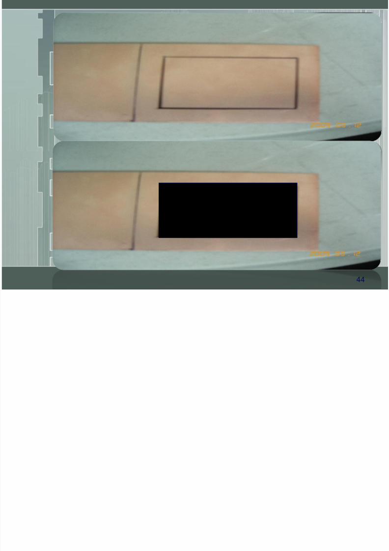
•After the modeling of the probe feed patch antenna andachieving satisfactory results we came to our fabricationpart.
•For this purpose we etched two antennas. To learn howpatch antennas are built we constructed one antennaourselves
•In order to get more accurate results we got one antennaetched from Allied electronics Lahore.
43
8/4/2019 Patch Antenna Presentation (1)
http://slidepdf.com/reader/full/patch-antenna-presentation-1 44/51
44

8/4/2019 Patch Antenna Presentation (1)
http://slidepdf.com/reader/full/patch-antenna-presentation-1 45/51
F i n
al
s t e pt ow
ar d
s t h
ef a
b r i c at i on
45

8/4/2019 Patch Antenna Presentation (1)
http://slidepdf.com/reader/full/patch-antenna-presentation-1 46/51
N et w or
k An
al
yz er
•A network analyzer is an instrument usedto analyze theproperties of
electrical networks,especially thosepropertiesassociated with thereflection andtransmission ofelectrical signalsknown as scatteringparameters
(S-parameters).
•Network analyzersare used mostly athigh frequencies
46

8/4/2019 Patch Antenna Presentation (1)
http://slidepdf.com/reader/full/patch-antenna-presentation-1 47/51
R et ur nL o
s s o
f t h eAn
t enn
a
The following figure was obtained from the vector network analyzer.
The figure shows the return loss graph of the patchantenna we fabricated. The results came out to be
outstanding. Well beyond our expectations. The return lossgraph showed that the return loss at 1.82 GHz is -30.261 dB
47
Th f ll i fi h th V lt t di

8/4/2019 Patch Antenna Presentation (1)
http://slidepdf.com/reader/full/patch-antenna-presentation-1 48/51
V ol t
a g e S t an
d i n
gW
av
eR
at i o
( V
S WR
)
•The following figure shows the Voltage standingwave ratio of our patch antenna.
•The VSWR of any working antenna should notexceed 2.
•In our case the result came out to be veryoutstanding. At the resonant frequency of 1.82GHzthe VSWR comes out to be 1.0840.
48

8/4/2019 Patch Antenna Presentation (1)
http://slidepdf.com/reader/full/patch-antenna-presentation-1 49/51
B A
CK
V I E W ( GR
O U N
D P L ANE
) OF
P AT CH
ANT E NNA
49

8/4/2019 Patch Antenna Presentation (1)
http://slidepdf.com/reader/full/patch-antenna-presentation-1 50/51
F R
ONT
V I E W ( P AT CH
) OF P AT CH A
NT E NNA
50

8/4/2019 Patch Antenna Presentation (1)
http://slidepdf.com/reader/full/patch-antenna-presentation-1 51/51
As we progressed with the passage of time we had to facechallenges in different ways. If they wouldn‟t have been solved
timely we could not have achieved our goal. A brief review ofdifficulties during the whole project are summarized below.
• Unavailability of HFSS® • Very few people having knowledge of soft ware, so findingan instructor of this field was difficult and time consuming.
• Lack of antenna testing equipment in any of theeducational institutes.
• People who had knowledge of network analyzer atcomsats were busy with there own university commitments so
taking some time from them also became an isssue.
•This problem was solved after requesting to Dr.Shahid A.KhanDean comsats who requested the concerned person to helpus.