Patch to the Future: Unsupervised Visual Prediction

CVPR 2014 Oral

Outline

• 1. Introduction• 2. Methodology• 3. Experimental Result• 4. Conclusion and Future Work

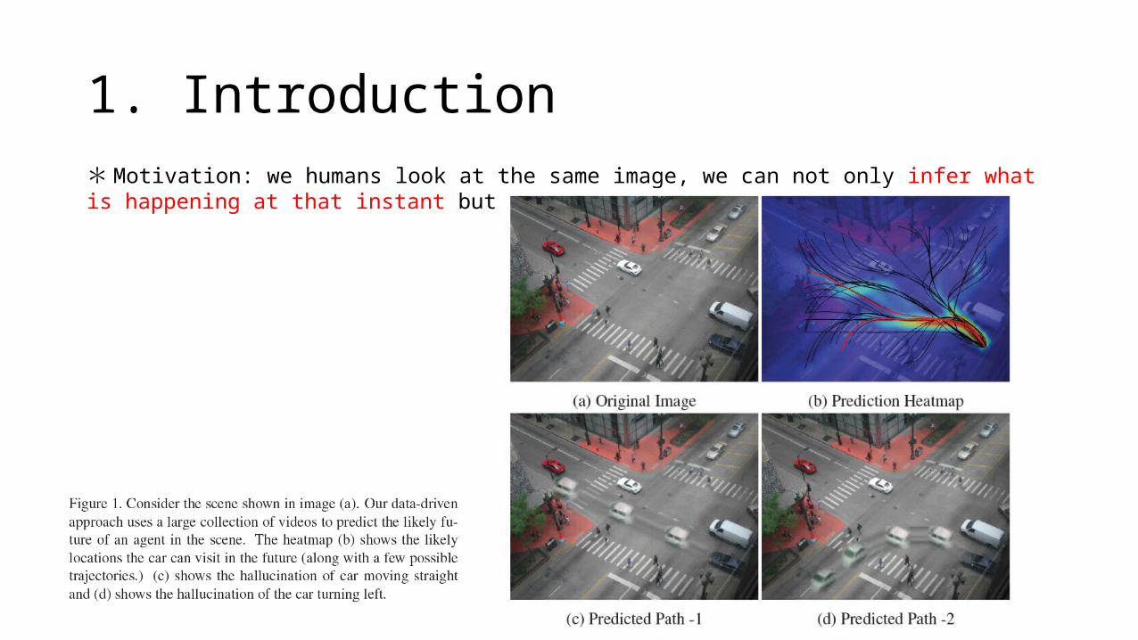
1. Introduction＊Motivation: we humans look at the same image, we can not only infer what is happening at that instant but also predict what can happen next.

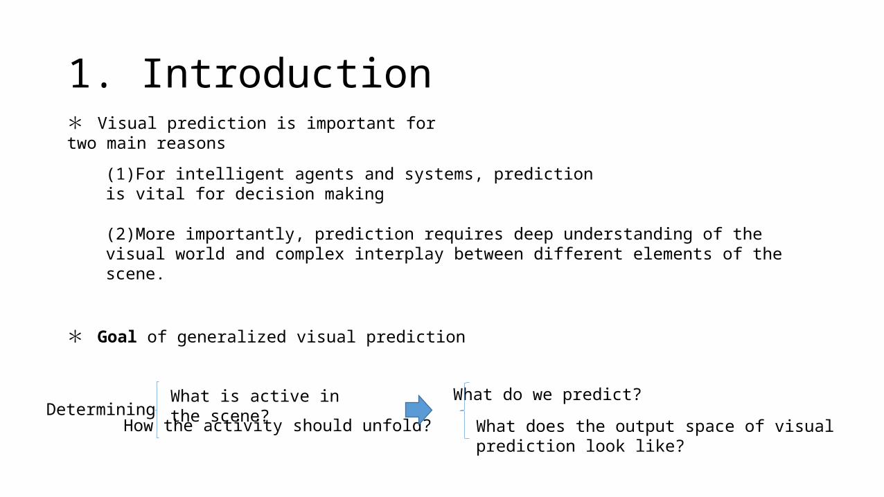
1. Introduction＊ Visual prediction is important for two main reasons

(1)For intelligent agents and systems, prediction is vital for decision making

(2)More importantly, prediction requires deep understanding of the visual world and complex interplay between different elements of the scene.

＊ Goal of generalized visual prediction

What is active in the scene?

How the activity should unfold?Determining

What do we predict?

What does the output space of visual prediction look like?

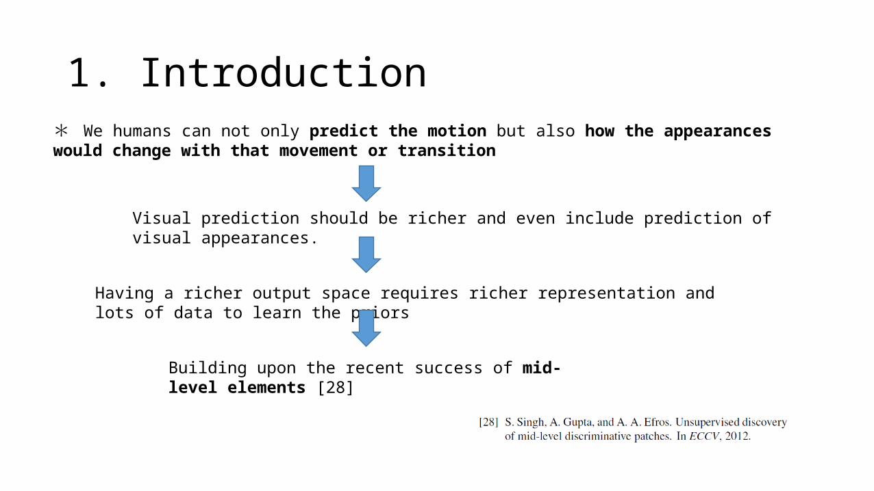
1. Introduction＊ We humans can not only predict the motion but also how the appearances would change with that movement or transition

Visual prediction should be richer and even include prediction of visual appearances.

Having a richer output space requires richer representation and lots of data to learn the priors

Building upon the recent success of mid-level elements [28]

1. Introduction＊ Advantages

No assumption about what can act as an agent and uses a data-driven approach to identify the possible agents and their activities

Using a patch-based representation allows us to learn the models of visual prediction in a completely unsupervised manner.

2. Methodology

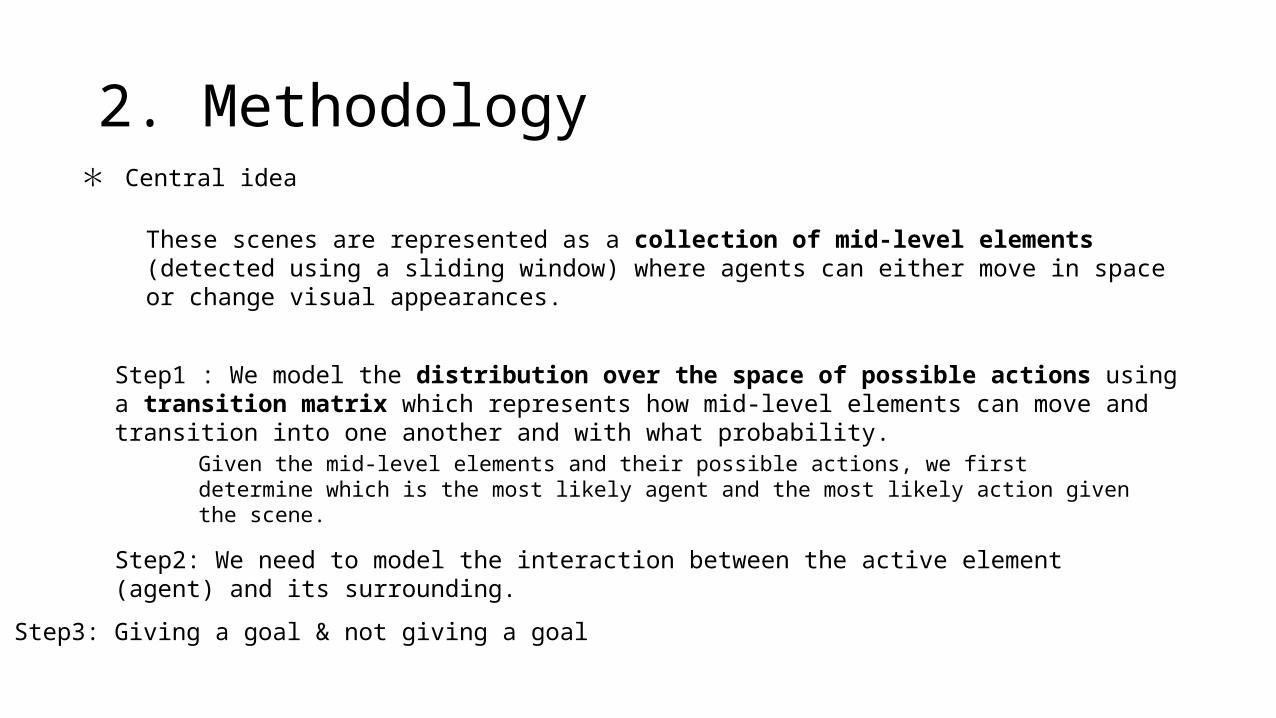
These scenes are represented as a collection of mid-level elements (detected using a sliding window) where agents can either move in space or change visual appearances.

＊ Central idea

Step1 : We model the distribution over the space of possible actions using a transition matrix which represents how mid-level elements can move and transition into one another and with what probability.

Step2: We need to model the interaction between the active element (agent) and its surrounding.

Given the mid-level elements and their possible actions, we first determine which is the most likely agent and the most likely action given the scene.

Step3: Giving a goal & not giving a goal

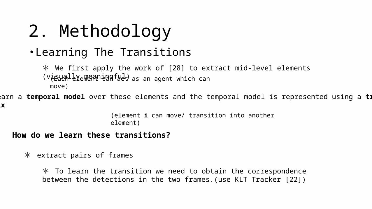
2. Methodology• Learning The Transitions

＊ We first apply the work of [28] to extract mid-level elements (visually meaningful)(Each element can act as an agent which can move)

＊ learn a temporal model over these elements and the temporal model is represented using a transitionmatrix

(element i can move/ transition into another element)

How do we learn these transitions?

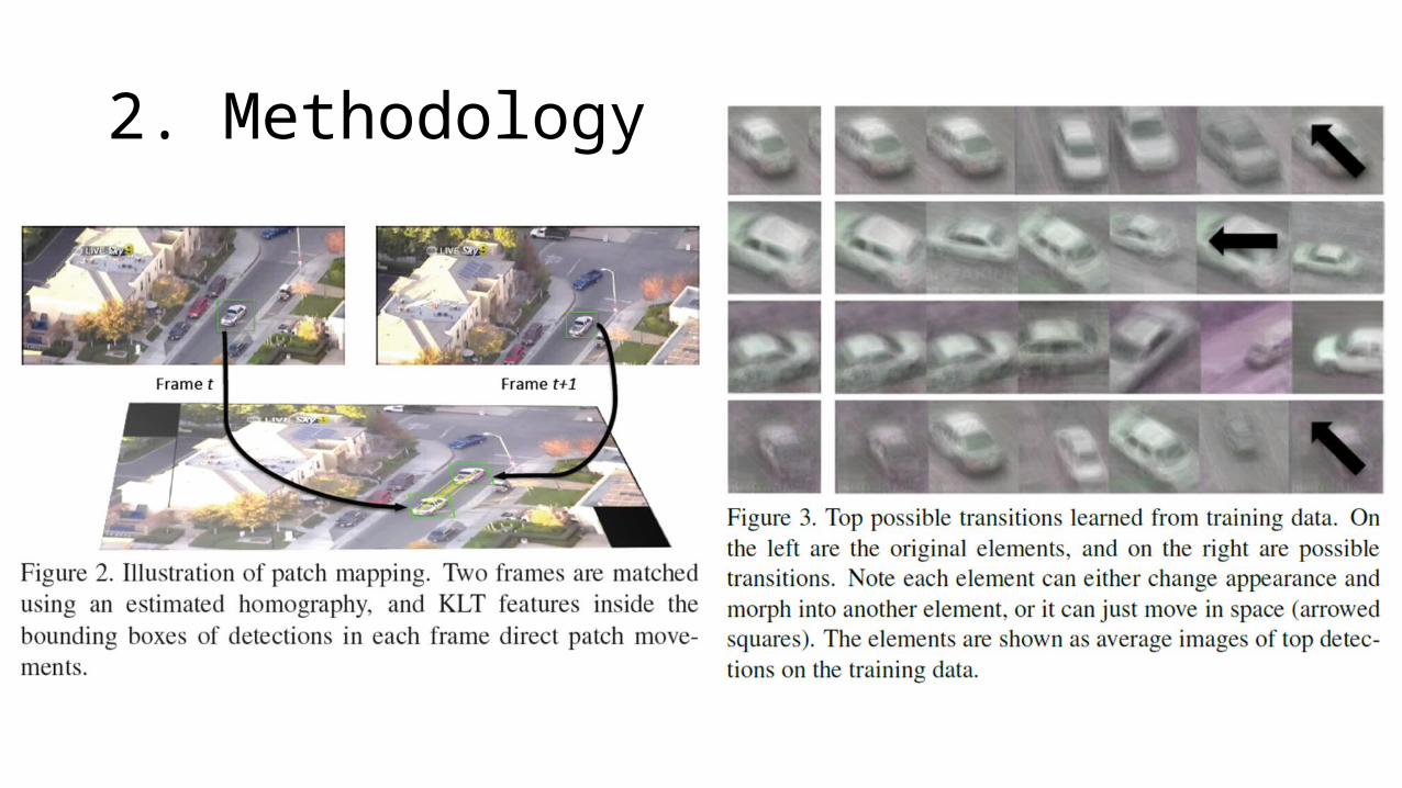
＊ extract pairs of frames

＊ To learn the transition we need to obtain the correspondence between the detections in the two frames.(use KLT Tracker [22])

2. Methodology＊ We interpret the mapping as either an appearance or spatial transition.

＊ In order to compensate for camera motion these movements are computed on a stitched panorama obtained via SIFT matching [21].

＊ For each transition, we normalize for total number of observed patches as well. This gives us the probability of transition for each mid-level patch.

2. Methodology

2. Methodology• Learning Contextual Information

＊ the actions of agents are not only dependent on likely transitions but also on the scene and the surroundings in which they appear

＊ We model these interactions using a reward function

(how likely is it that an element of type i can move to location (x, y) in the image)

＊ we learn a separate reward function for the interaction of each element within the scene

＊ To obtain the training data for reward function of element type i, we detect the element inthe training videos and observe which segments are likely to overlap with that element in time

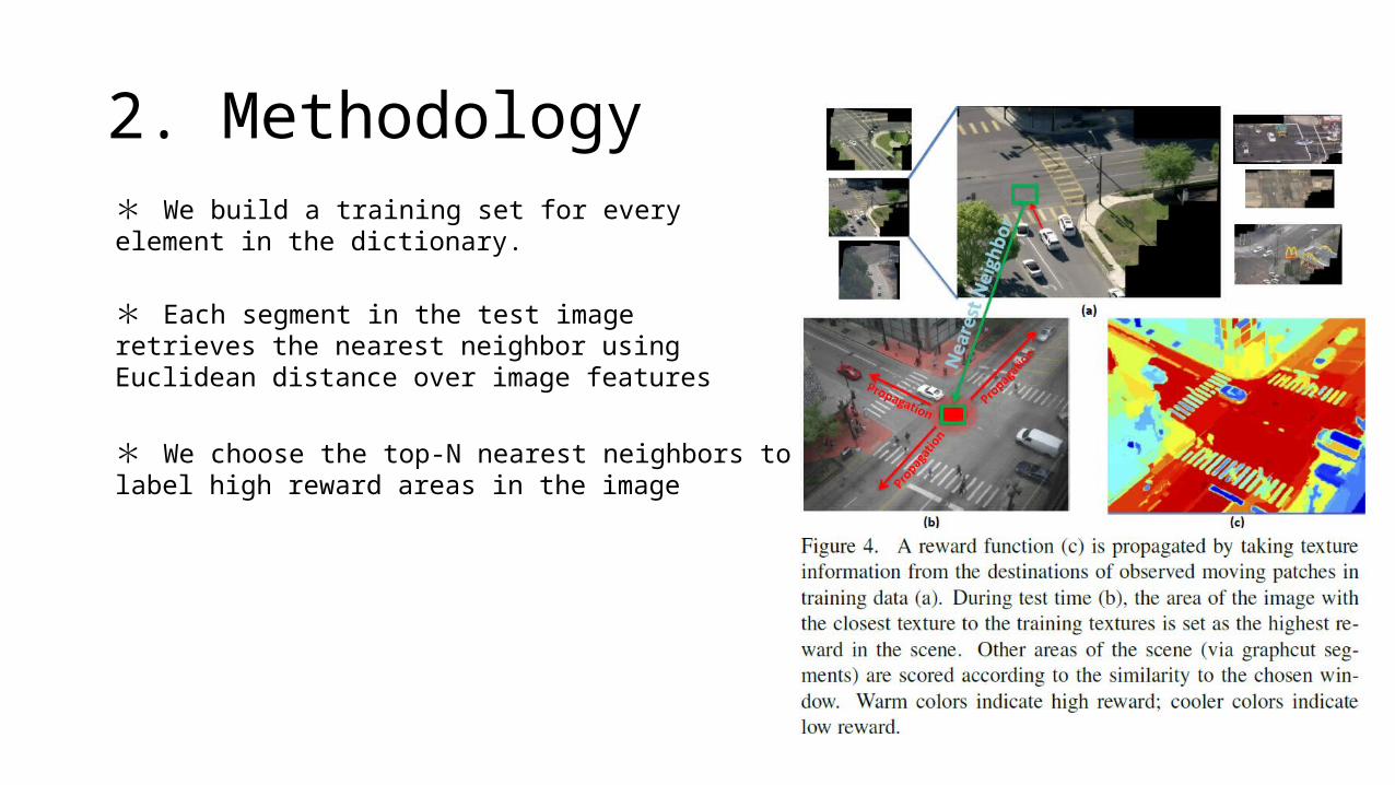
2. Methodology＊ We build a training set for every element in the dictionary.

＊ Each segment in the test image retrieves the nearest neighbor using Euclidean distance over image features

＊ We choose the top-N nearest neighbors to label high reward areas in the image

2. Methodology• Inferring Active Entities , Planning Actions and Choosing Goals

＊ Now we can predict what is going to happen next

＊ The prediction inference requires estimating the elements in the scene that are likely to be active

＊ we propose an automatic approach to infer the likely active agent based on the learned transition matrix

(Kitani et al. [18] choose the active agents manually)

＊ Our basic idea is to rank cluster types by their likelihood to be spatially active

＊ we first detect the instances of each element using sliding-window detection and then rank these instances based on contextual information.

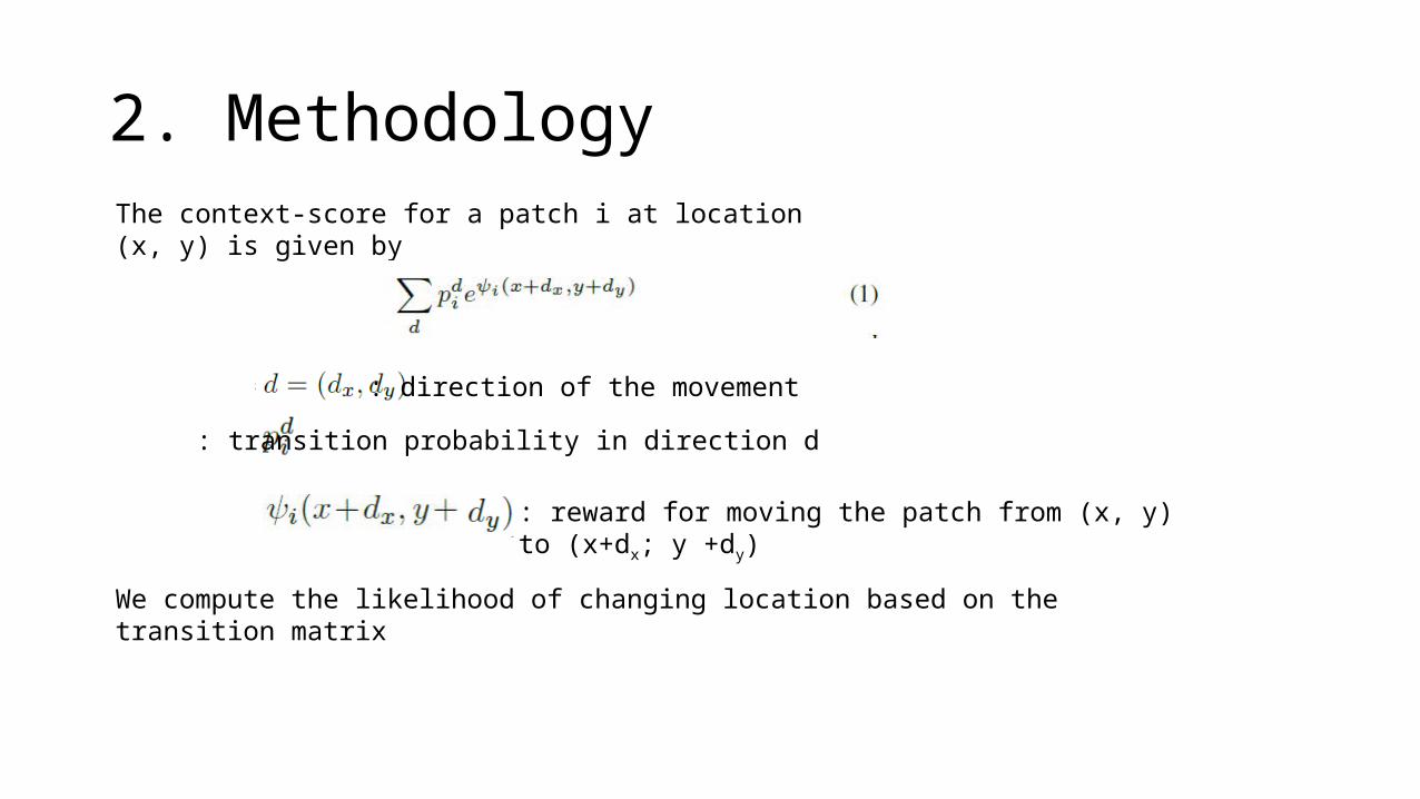
2. MethodologyThe context-score for a patch i at location (x, y) is given by

: direction of the movement

: transition probability in direction d

: reward for moving the patch from (x, y) to (x+dx; y +dy)

We compute the likelihood of changing location based on the transition matrix

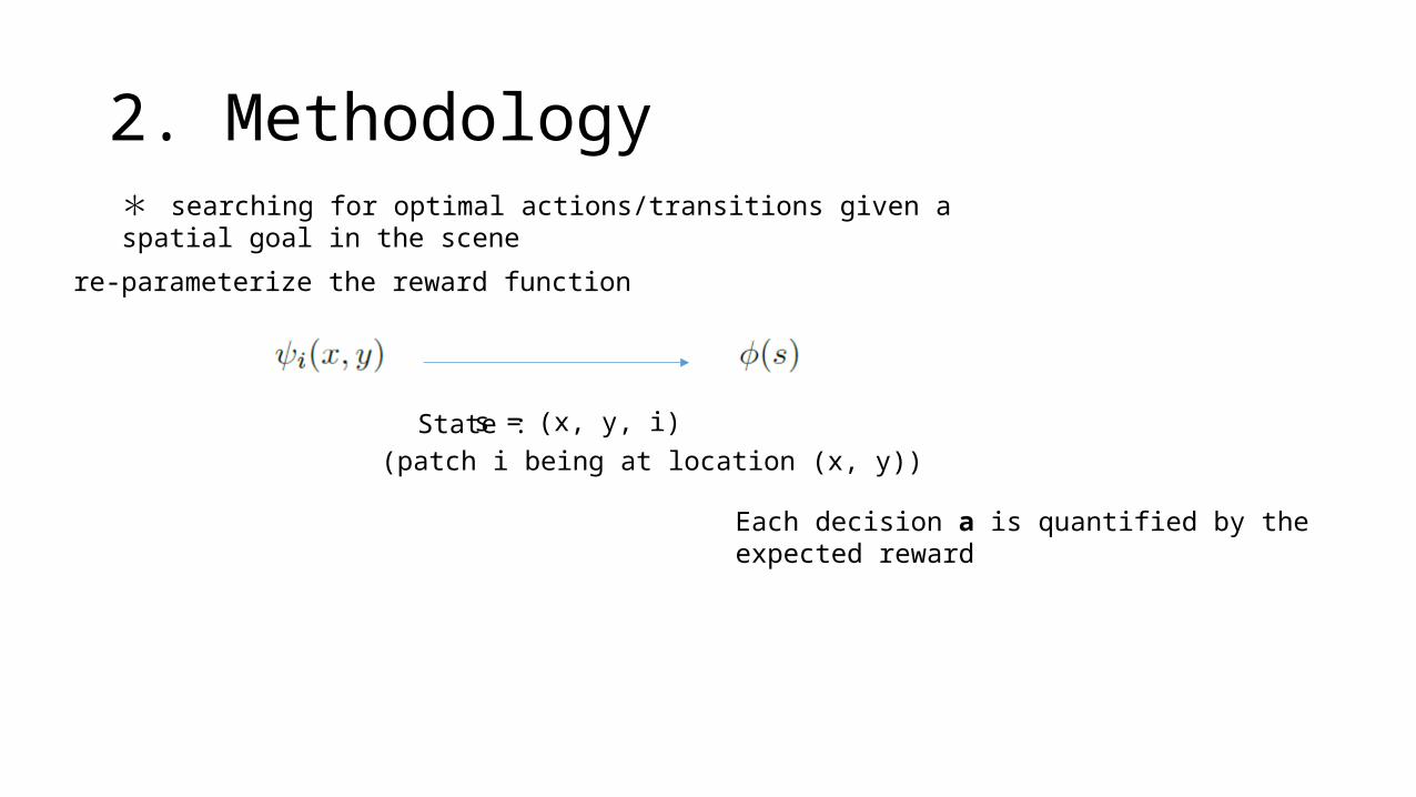
2. Methodology＊ searching for optimal actions/transitions given a spatial goal in the scene

re-parameterize the reward function

s = (x, y, i)(patch i being at location (x, y))

State :

Each decision a is quantified by the expected reward

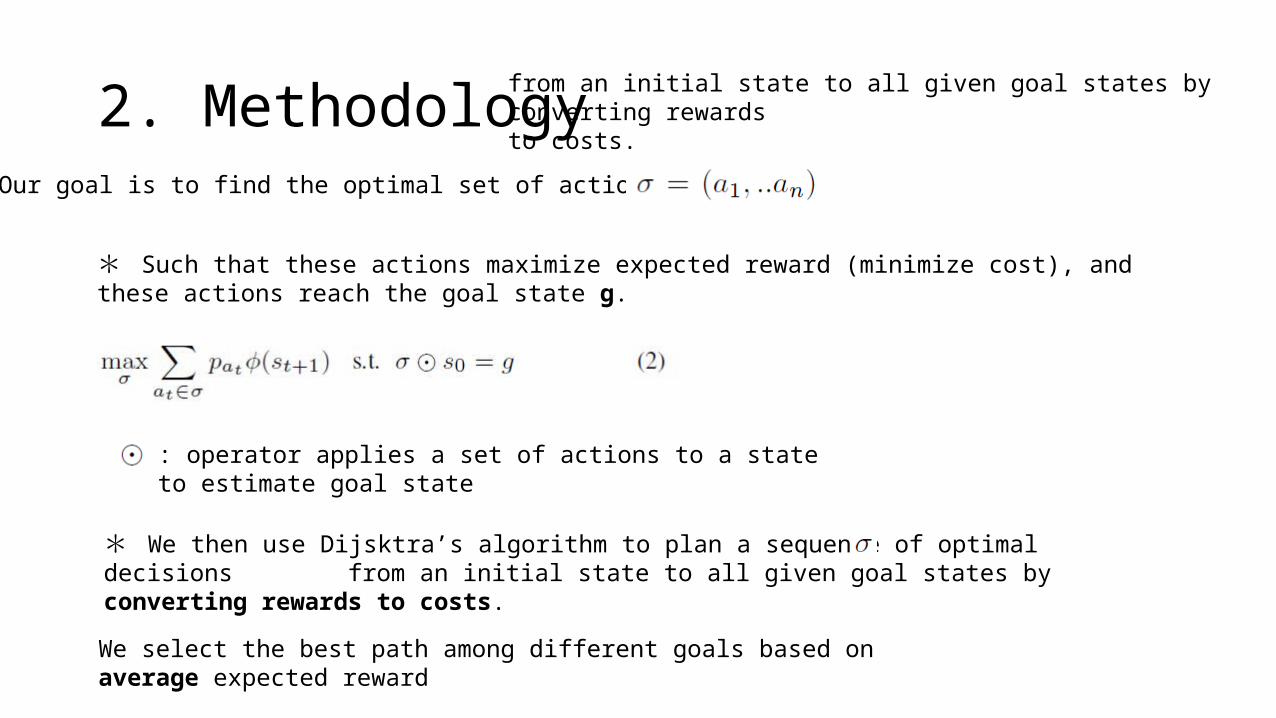
2. Methodology＊ Our goal is to find the optimal set of actions/decisions

＊ Such that these actions maximize expected reward (minimize cost), and these actions reach the goal state g.

: operator applies a set of actions to a state to estimate goal state

＊ We then use Dijsktra’s algorithm to plan a sequence of optimal decisions from an initial state to all given goal states by converting rewards to costs.

from an initial state to all given goal states by converting rewardsto costs.

We select the best path among different goals based on average expected reward

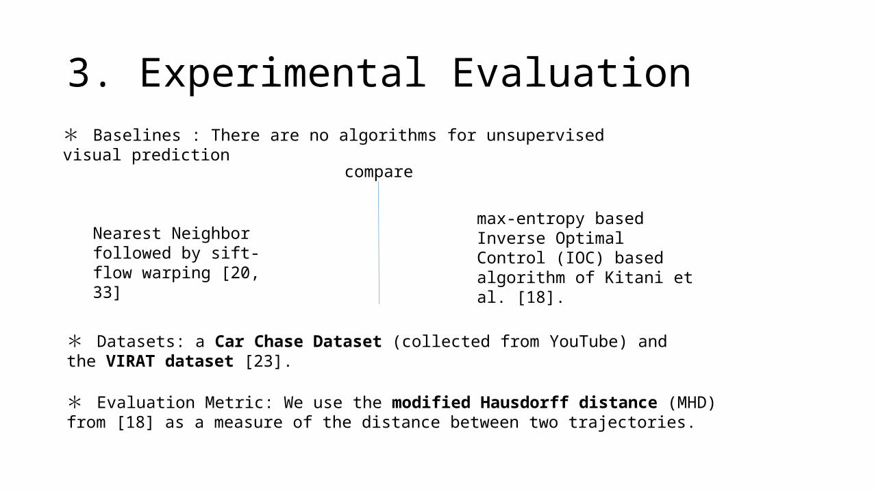
3. Experimental Evaluation＊ Baselines : There are no algorithms for unsupervised visual prediction

Nearest Neighbor followed by sift-flow warping [20, 33]

max-entropy based Inverse Optimal Control (IOC) based algorithm of Kitani et al. [18].

compare

＊ Datasets: a Car Chase Dataset (collected from YouTube) and the VIRAT dataset [23].

＊ Evaluation Metric: We use the modified Hausdorff distance (MHD) from [18] as a measure of the distance between two trajectories.

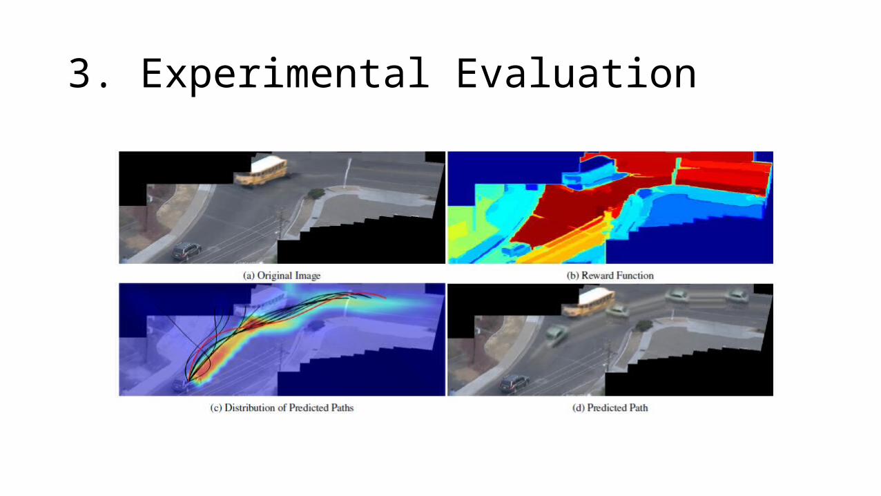
3. Experimental Evaluation

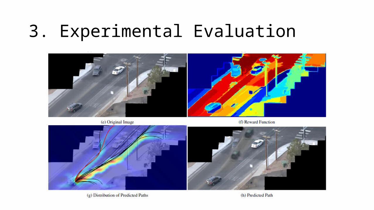
3. Experimental Evaluation

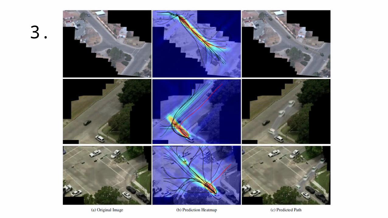
3. Experimental Evaluation

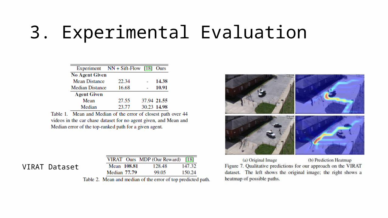
3. Experimental Evaluation

VIRAT Dataset

4. Conclusion and Future Work

＊ we have presented a simple and effective framework for visual prediction on a static scene.

＊ This representation allows us to train our framework in a completely unsupervised manner from a large collection of videos.

＊ Possible future work includes modeling the simultaneous behavior of multiple elements