Embed Size (px)
Citation preview
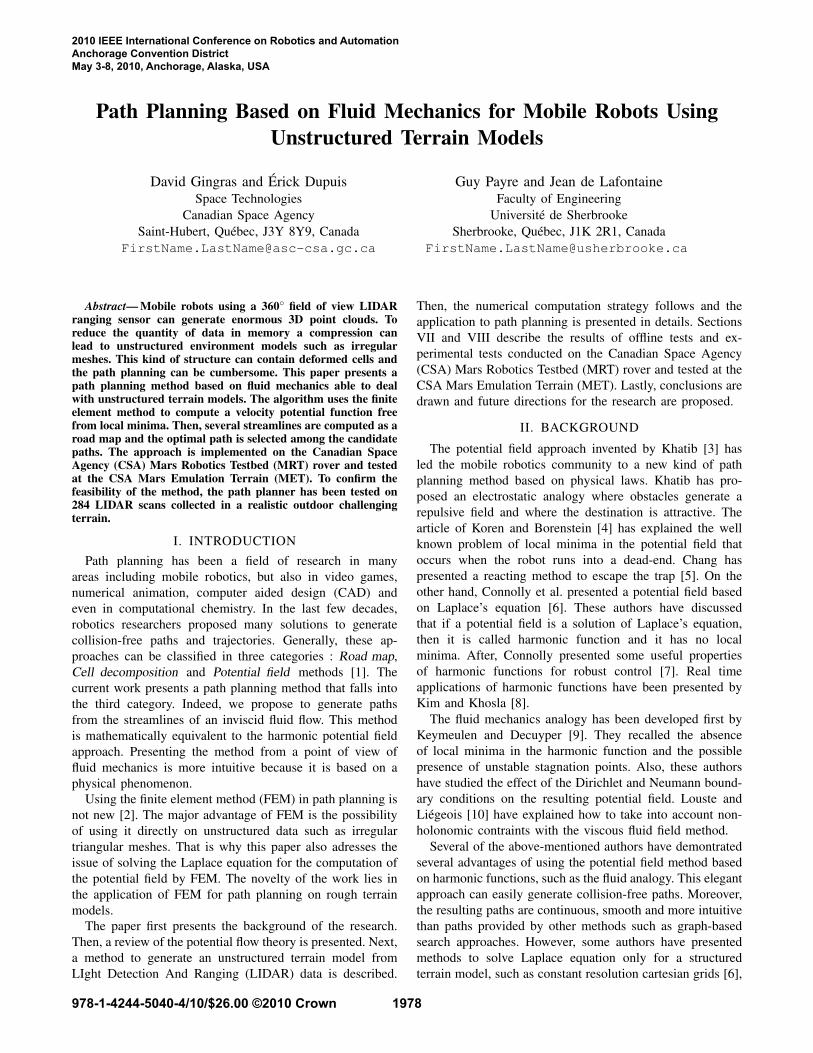
Path Planning Based on Fluid Mechanics for Mobile Robots UsingUnstructured Terrain Models
David Gingras and Erick DupuisSpace Technologies
Canadian Space Agency
Saint-Hubert, Quebec, J3Y 8Y9, Canada
Guy Payre and Jean de LafontaineFaculty of Engineering
Universite de Sherbrooke
Sherbrooke, Quebec, J1K 2R1, Canada
Abstract— Mobile robots using a 360◦ field of view LIDARranging sensor can generate enormous 3D point clouds. Toreduce the quantity of data in memory a compression canlead to unstructured environment models such as irregularmeshes. This kind of structure can contain deformed cells andthe path planning can be cumbersome. This paper presents apath planning method based on fluid mechanics able to dealwith unstructured terrain models. The algorithm uses the finiteelement method to compute a velocity potential function freefrom local minima. Then, several streamlines are computed as aroad map and the optimal path is selected among the candidatepaths. The approach is implemented on the Canadian SpaceAgency (CSA) Mars Robotics Testbed (MRT) rover and testedat the CSA Mars Emulation Terrain (MET). To confirm thefeasibility of the method, the path planner has been tested on284 LIDAR scans collected in a realistic outdoor challengingterrain.
I. INTRODUCTION
Path planning has been a field of research in many
areas including mobile robotics, but also in video games,
numerical animation, computer aided design (CAD) and
even in computational chemistry. In the last few decades,
robotics researchers proposed many solutions to generate
collision-free paths and trajectories. Generally, these ap-
proaches can be classified in three categories : Road map,
Cell decomposition and Potential field methods [1]. The
current work presents a path planning method that falls into
the third category. Indeed, we propose to generate paths
from the streamlines of an inviscid fluid flow. This method
is mathematically equivalent to the harmonic potential field
approach. Presenting the method from a point of view of
fluid mechanics is more intuitive because it is based on a
physical phenomenon.
Using the finite element method (FEM) in path planning is
not new [2]. The major advantage of FEM is the possibility
of using it directly on unstructured data such as irregular
triangular meshes. That is why this paper also adresses the
issue of solving the Laplace equation for the computation of
the potential field by FEM. The novelty of the work lies in
the application of FEM for path planning on rough terrain
models.
The paper first presents the background of the research.
Then, a review of the potential flow theory is presented. Next,
a method to generate an unstructured terrain model from
LIght Detection And Ranging (LIDAR) data is described.
Then, the numerical computation strategy follows and the
application to path planning is presented in details. Sections
VII and VIII describe the results of offline tests and ex-
perimental tests conducted on the Canadian Space Agency
(CSA) Mars Robotics Testbed (MRT) rover and tested at the
CSA Mars Emulation Terrain (MET). Lastly, conclusions are
drawn and future directions for the research are proposed.
II. BACKGROUND
The potential field approach invented by Khatib [3] has
led the mobile robotics community to a new kind of path
planning method based on physical laws. Khatib has pro-
posed an electrostatic analogy where obstacles generate a
repulsive field and where the destination is attractive. The
article of Koren and Borenstein [4] has explained the well
known problem of local minima in the potential field that
occurs when the robot runs into a dead-end. Chang has
presented a reacting method to escape the trap [5]. On the
other hand, Connolly et al. presented a potential field based
on Laplace’s equation [6]. These authors have discussed
that if a potential field is a solution of Laplace’s equation,
then it is called harmonic function and it has no local
minima. After, Connolly presented some useful properties
of harmonic functions for robust control [7]. Real time
applications of harmonic functions have been presented by
Kim and Khosla [8].
The fluid mechanics analogy has been developed first by
Keymeulen and Decuyper [9]. They recalled the absence
of local minima in the harmonic function and the possible
presence of unstable stagnation points. Also, these authors
have studied the effect of the Dirichlet and Neumann bound-
ary conditions on the resulting potential field. Louste and
Liegeois [10] have explained how to take into account non-
holonomic contraints with the viscous fluid field method.
Several of the above-mentioned authors have demontrated
several advantages of using the potential field method based
on harmonic functions, such as the fluid analogy. This elegant
approach can easily generate collision-free paths. Moreover,
the resulting paths are continuous, smooth and more intuitive
than paths provided by other methods such as graph-based
search approaches. However, some authors have presented
methods to solve Laplace equation only for a structured
terrain model, such as constant resolution cartesian grids [6],
2010 IEEE International Conference on Robotics and AutomationAnchorage Convention DistrictMay 3-8, 2010, Anchorage, Alaska, USA
978-1-4244-5040-4/10/$26.00 ©2010 Crown 1978
[10] and [11]. Most of them use the standard finite differencemethod to solve the Laplace equation. This approach is built
to work only on a structured grid which is not always the
best selection for a complex terrain model. This shortcoming
was adressed by Pimenta and co-workers [2] with the first
application of the FEM to robotics path planning.
The work presented in this paper uses an approach of
path plannig based on fluid mechanics, which is able to
take as input unstructured and uneven terrain models based
on irregular meshes. The motivation for using an irregular
mesh came from the compression of the enormous amount
of data provided by a 360◦ LIDAR scan. To store in memory
all the rover surrounding data, it is sufficient to generate
a mesh from LIDAR data and simplify it via a mesh
simplification algorithm, which reduces the number of cells
while preserving the shape and topography [12], [13] and
[14]. The resulting mesh is compact but unstructured because
it contains cells of different sizes and geometry. The standard
finite difference method cannot be used on this kind of terrain
model. That is why FEM is adopted here to solve the Laplace
equation. Differently from Pimenta et al., who also used
FEM, the present work generates a feasible road map and
selects an optimal path. Moreover, another improvement with
respect to previous works is the application of FEM to rough
and uneven terrain models.
III. POTENTIAL FLOW THEORY
Let us outline the mathematical model describing the
flow of an inviscid incompressible fluid. Assuming a steady
irrotational flow in the Eulerian framework, the velocity field
V obeys the relation
∇×V = 0. (1)
As a consequence, velocity is the gradient of a scalar
(potential) function φ , V =−∇φ . Conservation of mass for a
steady incompressible flow results in the expression ∇ ·V = 0,
so that the potential φ is harmonic (solution of the Laplace
equation)
∇2φ = 0, (2)
inside any volume where conservation of mass holds. A
localized fluid source (or a sink) can be modeled by a Dirac
term (δ ) added to the right hand side of (2). Assuming a unit
amount of fluid injected at point A during a unit of time and
the same unit withdrawn at point B, the velocity potential is
now solution of the Poisson equation:
−∇2φ = δA−δB. (3)
Equation (3) must be complemented by appropriate boundary
conditions. The fluid cannot flow through the boundaries, a
condition expressed by V ·n = 0 (n being a vector normal to
the boundary Γ). On Γ the velocity potential must verify:
∇φ ·n = 0, (4)
which amounts to the Neumann boundary conditions:
∂φ∂n
∣∣∣∣Γ
= 0. (5)
Resolution of the Poisson equation can be achieved by
several approaches. Section V explains how to obtain the
potential φ of (3) on an irregular triangular mesh (ITM).
The next step is the computation of the velocity field. As
explained before, the velocity of the flow can be computed
everywhere on the domain by the gradient of the potential.
For path planning purposes, the magnitude of velocity vec-
tors is not useful (only the direction is needed) and the vector
field V can be normalized.
IV. UNSTRUCTURED TERRAIN MODEL
This Section presents a strategy to get a terrain model
from a raw point cloud provided by a 360◦ LIDAR sensor
[14]. The model is an input of the path planning algorithm.
The complexity of the model must remain low in order to
limit the path planning computational time. The complexity
of the model is a tradeoff betwen computational time and
accuracy.
A. Mesh building and processing
When raw LIDAR data are acquired, an ITM is built from
the 3D point cloud. The approach is explained in details
in [14]. The triangular mesh is obtained using the Delaunaytriangulation [15] applied on the point cloud expressed in po-
lar coordinates. The resulting mesh can contain thousands of
triangles depending on the resolution of the raw scan. Then,
in order to reduce the quantity of redundant information, the
mesh is compressed via a simplification method using QSlimalgorithm [16].
To keep only the navigable region of the ITM, a filter
removes the triangles whose slope is too steep. This step
leads to a mesh without “walls” and “ceilling” and where
only the terrain without rocks and inclines is preserved. Then
a Laplacian smoothing filter is applied to improve the mesh
quality. Figure 1 shows an example of an ITM built from a
real LIDAR scan taken by the CSA MRT at the MET.
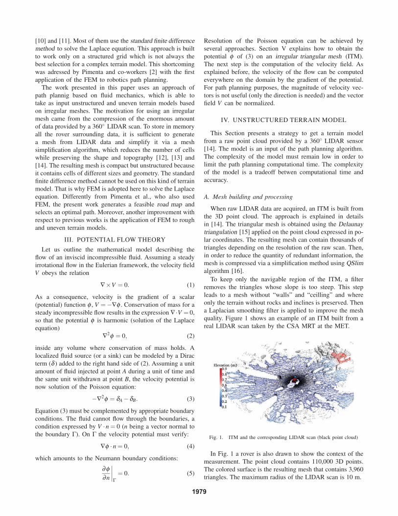
Fig. 1. ITM and the corresponding LIDAR scan (black point cloud)
In Fig. 1 a rover is also drawn to show the context of the
measurement. The point cloud contains 110,000 3D points.
The colored surface is the resulting mesh that contains 3,960
triangles. The maximum radius of the LIDAR scan is 10 m.
1979
V. NUMERICAL COMPUTATION
This Section deals with the numerical approximation of
the velocity field on a triangular mesh . One has first to
compute the potential φ , solution of the Poisson equation,
deducing next the velocity field V .
A. Approximation of the potential
For decades, the finite element method has been widely
used for the computation of potential functions. This paper
does not provide details of the method (the reader can refer to
[17] for further details). The FEM splits the domain into a fi-
nite set of cells, assuming a given (usually polynomial) shape
of the state function inside each cell. This discretization
reduces the problem to the computation of a finite number of
unknowns, which is performed by solving a linear system. In
our case, we can make direct use of the unstructured mesh
data obtained in the previous step as input to a finite element
solver. Using a linear Lagrange interpolation inside each
triangle e with vertices (i, j,k), the approximated potential
takes the form:
φ e(x,y) = φiNei (x,y)+φ jNe
j (x,y)+φkNek (x,y), (6)
where the shape function Nei is linear inside each cell, Ne
itakes the value 1 on vertex i and is equal to 0 for all other
mesh vertices. Fig. 2 presents an example of FEM problem
for a first order triangular mesh.
∇2φ=0
q=+δ
∂φ∂n=0
q=-δ
Fig. 2. Example of FEM problem with one source and one sink on asimple mesh
Figure 2 outlines the problem of potential flow according
to (3). There are a source with a positive volumetric flow
(represented by ⊗ with q = +δ ) and a sink (indicated by
� with q = −δ ). Elsewhere, the Laplacian of the potential
is zero (q = 0). Moreover, homogeneous Neumann boundary
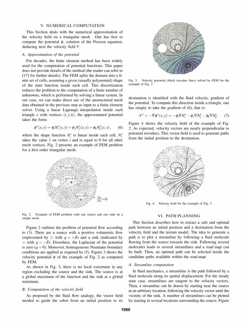
conditions are applied as required by (5). Figure 3 shows the
velocity potential φ of the example of Fig. 2 as computed
by FEM.
As shown in Fig. 3, there is no local extremum in any
region excluding the source and the sink. The source is at
a global maximum of the function and the sink at a global
minimum.
B. Computation of the velocity field
As proposed by the fluid flow analogy, the vector field
needed to guide the robot from an initial position to its
Fig. 3. Velocity potential (black isovalue lines) solved by FEM for theexample of Fig. 2
destination is identified with the fluid velocity, gradient of
the potential. To compute this direction inside a triangle, one
has simply to take the gradient of (6), that is:
V e =−∇φ e(x,y) =−φi∇Nei −φ j∇Ne
j −φk∇Nek . (7)
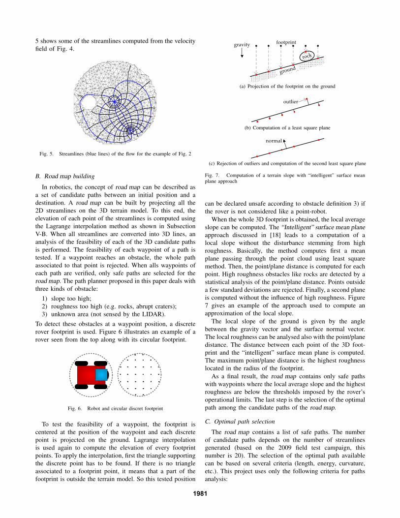
Figure 4 shows the velocity field of the example of Fig.
2. As expected, velocity vectors are nearly perpendicular to
potential isovalues. This vector field is used to generate paths
from the initial position to the destination.
Fig. 4. Velocity field for the example of Fig. 2
VI. PATH PLANNING
This Section describes how to extract a safe and optimal
path between an initial position and a destination from the
velocity field and the terrain model. The idea to generate a
path is to plot a streamline by following a fluid molecule
flowing from the source towards the sink. Following several
molecules leads to several streamlines and a road map can
be built. Then, an optimal path can be selected inside the
candidate paths available within the road map.
A. Streamline computation
In fluid mechanics, a streamline is the path followed by a
fluid molecule along its spatial displacement. For the steady
state case, streamlines are tangent to the velocity vectors.
Then, a streamline can be drawn by starting near the source
at an arbitrary location, following the velocity vector until the
vicinity of the sink. A number of streamlines can be plotted
by starting in several locations surrounding the source. Figure
1980
5 shows some of the streamlines computed from the velocity
field of Fig. 4.
Fig. 5. Streamlines (blue lines) of the flow for the example of Fig. 2
B. Road map building
In robotics, the concept of road map can be described as
a set of candidate paths between an initial position and a
destination. A road map can be built by projecting all the
2D streamlines on the 3D terrain model. To this end, the
elevation of each point of the streamlines is computed using
the Lagrange interpolation method as shown in Subsection
V-B. When all streamlines are converted into 3D lines, an
analysis of the feasibility of each of the 3D candidate paths
is performed. The feasibility of each waypoint of a path is
tested. If a waypoint reaches an obstacle, the whole path
associated to that point is rejected. When alls waypoints of
each path are verified, only safe paths are selected for the
road map. The path planner proposed in this paper deals with
three kinds of obstacle:
1) slope too high;
2) roughness too high (e.g. rocks, abrupt craters);
3) unknown area (not sensed by the LIDAR).
To detect these obstacles at a waypoint position, a discrete
rover footprint is used. Figure 6 illustrates an example of a
rover seen from the top along with its circular footprint.
Fig. 6. Robot and circular discret footprint
To test the feasibility of a waypoint, the footprint is
centered at the position of the waypoint and each discrete
point is projected on the ground. Lagrange interpolation
is used again to compute the elevation of every footprint
points. To apply the interpolation, first the triangle supporting
the discrete point has to be found. If there is no triangle
associated to a footprint point, it means that a part of the
footprint is outside the terrain model. So this tested position
rock
ground
footprintgravity
(a) Projection of the footprint on the ground
outlier
(b) Computation of a least square plane
normal
(c) Rejection of outliers and computation of the second least square plane
Fig. 7. Computation of a terrain slope with “intelligent” surface meanplane approach
can be declared unsafe according to obstacle definition 3) if
the rover is not considered like a point-robot.
When the whole 3D footprint is obtained, the local average
slope can be computed. The “Intelligent” surface mean planeapproach discussed in [18] leads to a computation of a
local slope without the disturbance stemming from high
roughness. Basically, the method computes first a mean
plane passing through the point cloud using least square
method. Then, the point/plane distance is computed for each
point. High roughness obstacles like rocks are detected by a
statistical analysis of the point/plane distance. Points outside
a few standard deviations are rejected. Finally, a second plane
is computed without the influence of high roughness. Figure
7 gives an example of the approach used to compute an
approximation of the local slope.
The local slope of the ground is given by the angle
between the gravity vector and the surface normal vector.
The local roughness can be analysed also with the point/plane
distance. The distance between each point of the 3D foot-
print and the “intelligent” surface mean plane is computed.
The maximum point/plane distance is the highest roughness
located in the radius of the footprint.
As a final result, the road map contains only safe paths
with waypoints where the local average slope and the highest
roughness are below the thresholds imposed by the rover’s
operational limits. The last step is the selection of the optimal
path among the candidate paths of the road map.
C. Optimal path selection
The road map contains a list of safe paths. The number
of candidate paths depends on the number of streamlines
generated (based on the 2009 field test campaign, this
number is 20). The selection of the optimal path available
can be based on several criteria (length, energy, curvature,
etc.). This project uses only the following criteria for paths
analysis:
1981
1) total length, and
2) energy consumption.
For each path of the road map, both criteria are computed
and two numbers can be associated to each path. One is
associated to the total length and the other is proportionnal
to the energy consumed to follow the path. The 3D length
l is simply computed as the sum of segments composing a
path:
l =n
∑i=2
‖Pi−Pi−1‖, (8)
where Pi is the 3D position vector of the waypoint i, and nis the number of waypoints for a path. For the analysis of
energy consumption, only the gravitational potential associ-
ated to change in elevation is considered. So for every paths,
the elevation gain lz+ is computed by:
lz+ =n
∑i=2
αi, (9)
where αi is defined as follows:
αi ={
Piz −Pi−1z , Piz −Pi−1z > 0 (10a)
0, otherwise. (10b)
The term Piz is the elevation of waypoint i. When all paths of
the road map are analysed with each criterion defined by (8)
and (9), a cost can be associated to each path. The values of
length and energy are normalized and indicated by l and lz+.
The cost C can be computed for each path with the following
expression:
C = βl l +βlz+ lz+ , (11)
where βl et βlz+are weighting positive values. Finally, the
selected path is the one with the lowest cost.
VII. REAL WORLD IMPLEMENTATION
This Section describes an implementation of the above
described path planner on the Canadian Space Agency Mars
Rover Testbed (MRT). The MRT is operated in an outdoor
laboratory (MET) of 60 m by 30 m that emulates the
topography of a martian terrain. MET features several rocks
of different dimensions, craters along with a mountain, a
plain, a cave and a cliff. The MRT is a modified Pioneer
P2AT mobile robot manifactured by ActivMedia. The rover
is equipped with a SICK LIDAR mounted on a rotating pan
unit leading to a 360◦ field of view vision sensor. The robot
has onboard a Panasonic Toughbook laptop with Intel Core
2 processor running Linux operating system. Figure 8 (a)
shows the CSA testbed. The high level autonomy algorithms
are coded in JAVA and implemented in Eclipse 3.5. The
path planner and the terrain modeler are coded in Matlab
scripts and deployed to JAVA with the Builder-JA Toolbox
of Mathworks. The finite element solver is coded in C-mexscript.
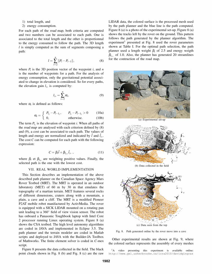
Figure 8 presents the data collected in the field. The black
point clouds shown in Fig. 8 (b) and Fig. 8 (c) are the raw
LIDAR data, the colored surface is the processed mesh used
by the path planner and the blue line is the path computed.
Figure 8 (a) is a photo of the experimental set-up. Figure 8 (a)
shows the tracks left by the rover on the ground. This pattern
follows the path generated by the planner algorithm. The
experiment1 presented at Fig. 8 used the rover parameters
shown at Table I. For the optimal path selection, the path
planner used a length weight βl of 2.5 and energy weigth
βlz+ of 1.0. Also, the planner has generated 20 streamlines
for the contruction of the road map.
(a) Experimental set-up
x
z
y
(b) Data collected in the field
y
x
(c) Data seen from the top
Fig. 8. Path generated online by the rover move into a cave
Other experimental results are shown at Fig. 9, where
the colored surface represents the assembly of every meshes
1A video presenting this experiment is available online:http://www.gel.usherbrooke.ca/icra2010/davidgingras
1982
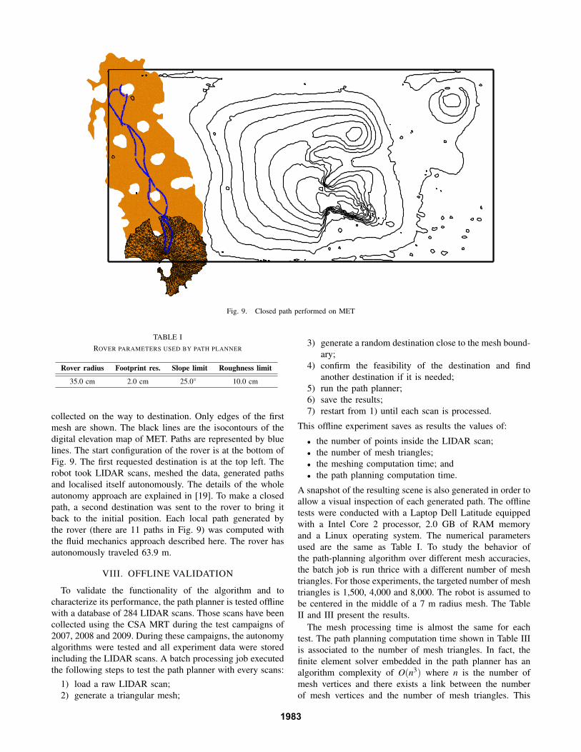
Fig. 9. Closed path performed on MET
TABLE I
ROVER PARAMETERS USED BY PATH PLANNER
Rover radius Footprint res. Slope limit Roughness limit
35.0 cm 2.0 cm 25.0◦ 10.0 cm
collected on the way to destination. Only edges of the first
mesh are shown. The black lines are the isocontours of the
digital elevation map of MET. Paths are represented by blue
lines. The start configuration of the rover is at the bottom of
Fig. 9. The first requested destination is at the top left. The
robot took LIDAR scans, meshed the data, generated paths
and localised itself autonomously. The details of the whole
autonomy approach are explained in [19]. To make a closed
path, a second destination was sent to the rover to bring it
back to the initial position. Each local path generated by
the rover (there are 11 paths in Fig. 9) was computed with
the fluid mechanics approach described here. The rover has
autonomously traveled 63.9 m.
VIII. OFFLINE VALIDATION
To validate the functionality of the algorithm and to
characterize its performance, the path planner is tested offline
with a database of 284 LIDAR scans. Those scans have been
collected using the CSA MRT during the test campaigns of
2007, 2008 and 2009. During these campaigns, the autonomy
algorithms were tested and all experiment data were stored
including the LIDAR scans. A batch processing job executed
the following steps to test the path planner with every scans:
1) load a raw LIDAR scan;
2) generate a triangular mesh;
3) generate a random destination close to the mesh bound-
ary;
4) confirm the feasibility of the destination and find
another destination if it is needed;
5) run the path planner;
6) save the results;
7) restart from 1) until each scan is processed.
This offline experiment saves as results the values of:
• the number of points inside the LIDAR scan;
• the number of mesh triangles;
• the meshing computation time; and
• the path planning computation time.
A snapshot of the resulting scene is also generated in order to
allow a visual inspection of each generated path. The offline
tests were conducted with a Laptop Dell Latitude equipped
with a Intel Core 2 processor, 2.0 GB of RAM memory
and a Linux operating system. The numerical parameters
used are the same as Table I. To study the behavior of
the path-planning algorithm over different mesh accuracies,
the batch job is run thrice with a different number of mesh
triangles. For those experiments, the targeted number of mesh
triangles is 1,500, 4,000 and 8,000. The robot is assumed to
be centered in the middle of a 7 m radius mesh. The Table
II and III present the results.
The mesh processing time is almost the same for each
test. The path planning computation time shown in Table III
is associated to the number of mesh triangles. In fact, the
finite element solver embedded in the path planner has an
algorithm complexity of O(n3) where n is the number of
mesh vertices and there exists a link between the number
of mesh vertices and the number of mesh triangles. This
1983
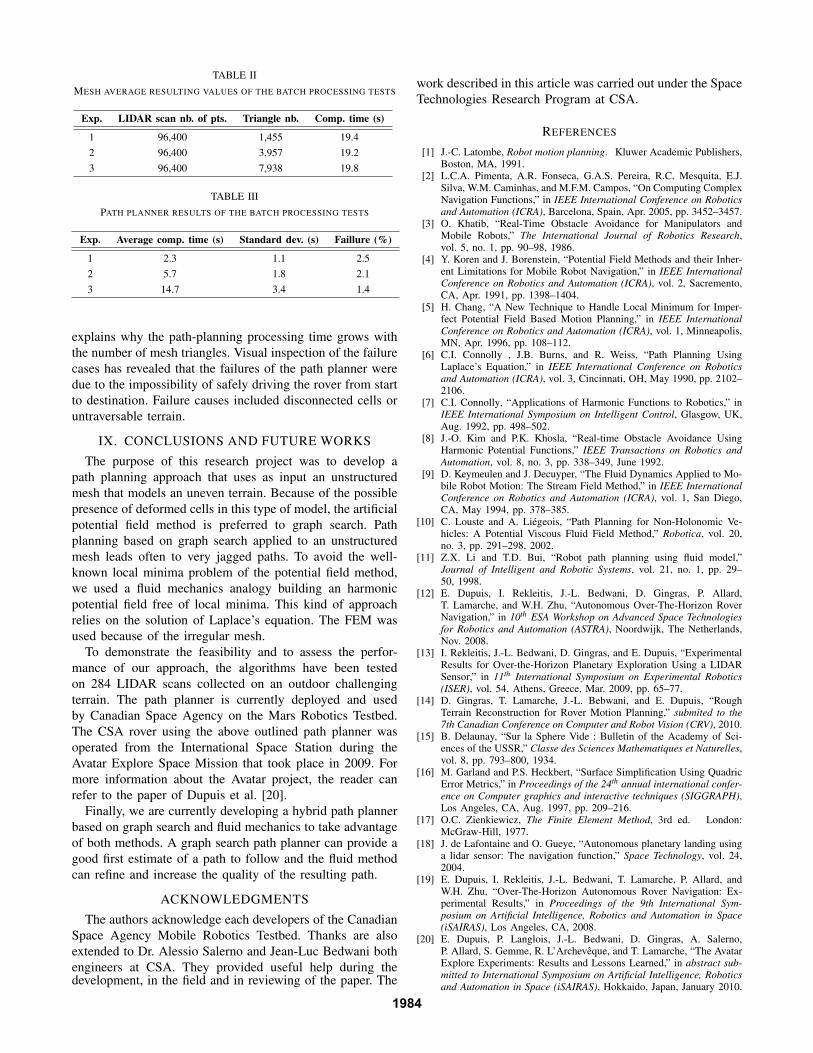
TABLE II
MESH AVERAGE RESULTING VALUES OF THE BATCH PROCESSING TESTS
Exp. LIDAR scan nb. of pts. Triangle nb. Comp. time (s)
1 96,400 1,455 19.4
2 96,400 3,957 19.2
3 96,400 7,938 19.8
TABLE III
PATH PLANNER RESULTS OF THE BATCH PROCESSING TESTS
Exp. Average comp. time (s) Standard dev. (s) Faillure (%)
1 2.3 1.1 2.5
2 5.7 1.8 2.1
3 14.7 3.4 1.4
explains why the path-planning processing time grows with
the number of mesh triangles. Visual inspection of the failure
cases has revealed that the failures of the path planner were
due to the impossibility of safely driving the rover from start
to destination. Failure causes included disconnected cells or
untraversable terrain.
IX. CONCLUSIONS AND FUTURE WORKS
The purpose of this research project was to develop a
path planning approach that uses as input an unstructured
mesh that models an uneven terrain. Because of the possible
presence of deformed cells in this type of model, the artificial
potential field method is preferred to graph search. Path
planning based on graph search applied to an unstructured
mesh leads often to very jagged paths. To avoid the well-
known local minima problem of the potential field method,
we used a fluid mechanics analogy building an harmonic
potential field free of local minima. This kind of approach
relies on the solution of Laplace’s equation. The FEM was
used because of the irregular mesh.
To demonstrate the feasibility and to assess the perfor-
mance of our approach, the algorithms have been tested
on 284 LIDAR scans collected on an outdoor challenging
terrain. The path planner is currently deployed and used
by Canadian Space Agency on the Mars Robotics Testbed.
The CSA rover using the above outlined path planner was
operated from the International Space Station during the
Avatar Explore Space Mission that took place in 2009. For
more information about the Avatar project, the reader can
refer to the paper of Dupuis et al. [20].
Finally, we are currently developing a hybrid path planner
based on graph search and fluid mechanics to take advantage
of both methods. A graph search path planner can provide a
good first estimate of a path to follow and the fluid method
can refine and increase the quality of the resulting path.
ACKNOWLEDGMENTS
The authors acknowledge each developers of the Canadian
Space Agency Mobile Robotics Testbed. Thanks are also
extended to Dr. Alessio Salerno and Jean-Luc Bedwani both
engineers at CSA. They provided useful help during thedevelopment, in the field and in reviewing of the paper. The
work described in this article was carried out under the Space
Technologies Research Program at CSA.
REFERENCES
[1] J.-C. Latombe, Robot motion planning. Kluwer Academic Publishers,Boston, MA, 1991.
[2] L.C.A. Pimenta, A.R. Fonseca, G.A.S. Pereira, R.C. Mesquita, E.J.Silva, W.M. Caminhas, and M.F.M. Campos, “On Computing ComplexNavigation Functions,” in IEEE International Conference on Roboticsand Automation (ICRA), Barcelona, Spain, Apr. 2005, pp. 3452–3457.
[3] O. Khatib, “Real-Time Obstacle Avoidance for Manipulators andMobile Robots,” The International Journal of Robotics Research,vol. 5, no. 1, pp. 90–98, 1986.
[4] Y. Koren and J. Borenstein, “Potential Field Methods and their Inher-ent Limitations for Mobile Robot Navigation,” in IEEE InternationalConference on Robotics and Automation (ICRA), vol. 2, Sacremento,CA, Apr. 1991, pp. 1398–1404.
[5] H. Chang, “A New Technique to Handle Local Minimum for Imper-fect Potential Field Based Motion Planning,” in IEEE InternationalConference on Robotics and Automation (ICRA), vol. 1, Minneapolis,MN, Apr. 1996, pp. 108–112.
[6] C.I. Connolly , J.B. Burns, and R. Weiss, “Path Planning UsingLaplace’s Equation,” in IEEE International Conference on Roboticsand Automation (ICRA), vol. 3, Cincinnati, OH, May 1990, pp. 2102–2106.
[7] C.I. Connolly, “Applications of Harmonic Functions to Robotics,” inIEEE International Symposium on Intelligent Control, Glasgow, UK,Aug. 1992, pp. 498–502.
[8] J.-O. Kim and P.K. Khosla, “Real-time Obstacle Avoidance UsingHarmonic Potential Functions,” IEEE Transactions on Robotics andAutomation, vol. 8, no. 3, pp. 338–349, June 1992.
[9] D. Keymeulen and J. Decuyper, “The Fluid Dynamics Applied to Mo-bile Robot Motion: The Stream Field Method,” in IEEE InternationalConference on Robotics and Automation (ICRA), vol. 1, San Diego,CA, May 1994, pp. 378–385.
[10] C. Louste and A. Liegeois, “Path Planning for Non-Holonomic Ve-hicles: A Potential Viscous Fluid Field Method,” Robotica, vol. 20,no. 3, pp. 291–298, 2002.
[11] Z.X. Li and T.D. Bui, “Robot path planning using fluid model,”Journal of Intelligent and Robotic Systems, vol. 21, no. 1, pp. 29–50, 1998.
[12] E. Dupuis, I. Rekleitis, J.-L. Bedwani, D. Gingras, P. Allard,T. Lamarche, and W.H. Zhu, “Autonomous Over-The-Horizon RoverNavigation,” in 10th ESA Workshop on Advanced Space Technologiesfor Robotics and Automation (ASTRA), Noordwijk, The Netherlands,Nov. 2008.
[13] I. Rekleitis, J.-L. Bedwani, D. Gingras, and E. Dupuis, “ExperimentalResults for Over-the-Horizon Planetary Exploration Using a LIDARSensor,” in 11th International Symposium on Experimental Robotics(ISER), vol. 54, Athens, Greece, Mar. 2009, pp. 65–77.
[14] D. Gingras, T. Lamarche, J.-L. Bebwani, and E. Dupuis, “RoughTerrain Reconstruction for Rover Motion Planning,” submited to the7th Canadian Conference on Computer and Robot Vision (CRV), 2010.
[15] B. Delaunay, “Sur la Sphere Vide : Bulletin of the Academy of Sci-ences of the USSR,” Classe des Sciences Mathematiques et Naturelles,vol. 8, pp. 793–800, 1934.
[16] M. Garland and P.S. Heckbert, “Surface Simplification Using QuadricError Metrics,” in Proceedings of the 24th annual international confer-ence on Computer graphics and interactive techniques (SIGGRAPH),Los Angeles, CA, Aug. 1997, pp. 209–216.
[17] O.C. Zienkiewicz, The Finite Element Method, 3rd ed. London:McGraw-Hill, 1977.
[18] J. de Lafontaine and O. Gueye, “Autonomous planetary landing usinga lidar sensor: The navigation function,” Space Technology, vol. 24,2004.
[19] E. Dupuis, I. Rekleitis, J.-L. Bedwani, T. Lamarche, P. Allard, andW.H. Zhu, “Over-The-Horizon Autonomous Rover Navigation: Ex-perimental Results,” in Proceedings of the 9th International Sym-posium on Artificial Intelligence, Robotics and Automation in Space(iSAIRAS), Los Angeles, CA, 2008.
[20] E. Dupuis, P. Langlois, J.-L. Bedwani, D. Gingras, A. Salerno,P. Allard, S. Gemme, R. L’Archeveque, and T. Lamarche, “The AvatarExplore Experiments: Results and Lessons Learned,” in abstract sub-mitted to International Symposium on Artificial Intelligence, Roboticsand Automation in Space (iSAIRAS), Hokkaido, Japan, January 2010.
1984