Embed Size (px)
Citation preview
Patrick F. Cunniff George J. O'Hara
University of Maryland College Park, MO 20742
Feasibility of a Transient Dynamic Design Analysis Method
This article addresses the degree of success that may be achieved by using simple equipment-vehicle models that produce time history responses whose equipment fixed base modal maximum response values are equivalent to those found in the u.s. Navy's dynamic design analysis method. The criteria of success is measured by a comparison of the results with typical interim shock design values. The equipment models reported are limited to two- degree and three degrees offreedom systems; the model of the vehicle to which the equipment is attached consists solely of a rigid mass and an elastic spring; and the shock excitation is produced by an ideal impulse that is applied to the vehicle mass. © 1994 John Wiley & Sons, Inc.
INTRODUCTION
The dynamic design analysis method (DDAM) (Belsheim and O'Hara, 1960), has been used for more than 30 years as part of the Navy's efforts to shock-harden heavy shipboard equipment. This spectral method, which has been validated several times (O'Hara, 1979), employs normal mode theory, modal effective mass (O'Hara and Cunniff, 1963, Cunniff and O'Hara, 1965), and design shock values (O'Hara and Belsheim, 1963). DDAM prescribes a modal analysis approach that utilizes these shock design values in three orthogonal directions and takes into account the type of vehicle and equipment location, that is, hull-mounted, deck-mounted, and shell-plate mounted. Recent articles have provided an overview on the evolution of spectral techniques in naval shock design (Remmers, 1983), guidance to account for structural interactive effects in choosing design shock values from shock spectra (O'Hara and Cunniff, 1985), and the demonstration of a procedure that utilizes modal effective weight (Cunniff and O'Hara,
Received January 25, 1993; Accepted August 18, 1993.
Shock and Vibration, Vol. 1, No.3, pp. 241-251 (1994) © 1994 John Wiley & Sons, Inc.
1989) for establishing shock design curves for spectral analysis from accumulated data.
Since its introduction, different transient analysis methods have been proposed as alternative approaches. The practice of using some "typical" base motion for a class of structural systems as a design input is flawed, sometimes grievously so. This is because during a shock, the base motion includes the interactive effects between the equipment and its supporting structure. Consequently, it is generally not useful as an input function for different equipment attached to the same supporting structure because the different interaction causes a different motion. Likewise, trying to average base motions obtained at different points of a multifoundation system can and does lead to a wide range of results that are in error. This is especially true when one compares shock design values derived from original base motions with those derived from average motions. Another method (Private communications, 1990), used a simple base mass to represent the vehicle to which the equipment is attached, and an impulsive force applied to the base mass to
CCC 1070-9622/94/030241-11
241
242 Cuniff and O'Hara
produce the shock motion excitation for the equipment. A recent article by O'Hara and Cunniff (1991) examined the degree of success that may be achieved by the simple model to produce time history base motions for the equipment responses whose modal maximum response values are the prescribed shock design values. The vehicle, modeled as a lumped mass, provided solutions when the ratio of the prescribed shock design values (mode 1 divided by mode 2) was less than unity. Solutions were unattainable when the same ratio of design inputs were equal to or greater than unity.
This study examines the situation when the vehicle model is a simple mass-spring system onto which a two or three degrees of freedom equipment is attached. The completed equipment-vehicle system is then excited by an impulse applied to the vehicle mass. The relative displacement of each equipment modal oscillator, scaled by its corresponding fixed base frequency, is compared to the shock design values. It will be shown that this new vehicle overcomes the shortcomings reported by O'Hara and Cunniff (1991) for two degrees of freedom equipment, and successfully accommodates the three degrees of freedom equipment.
BACKGROUND
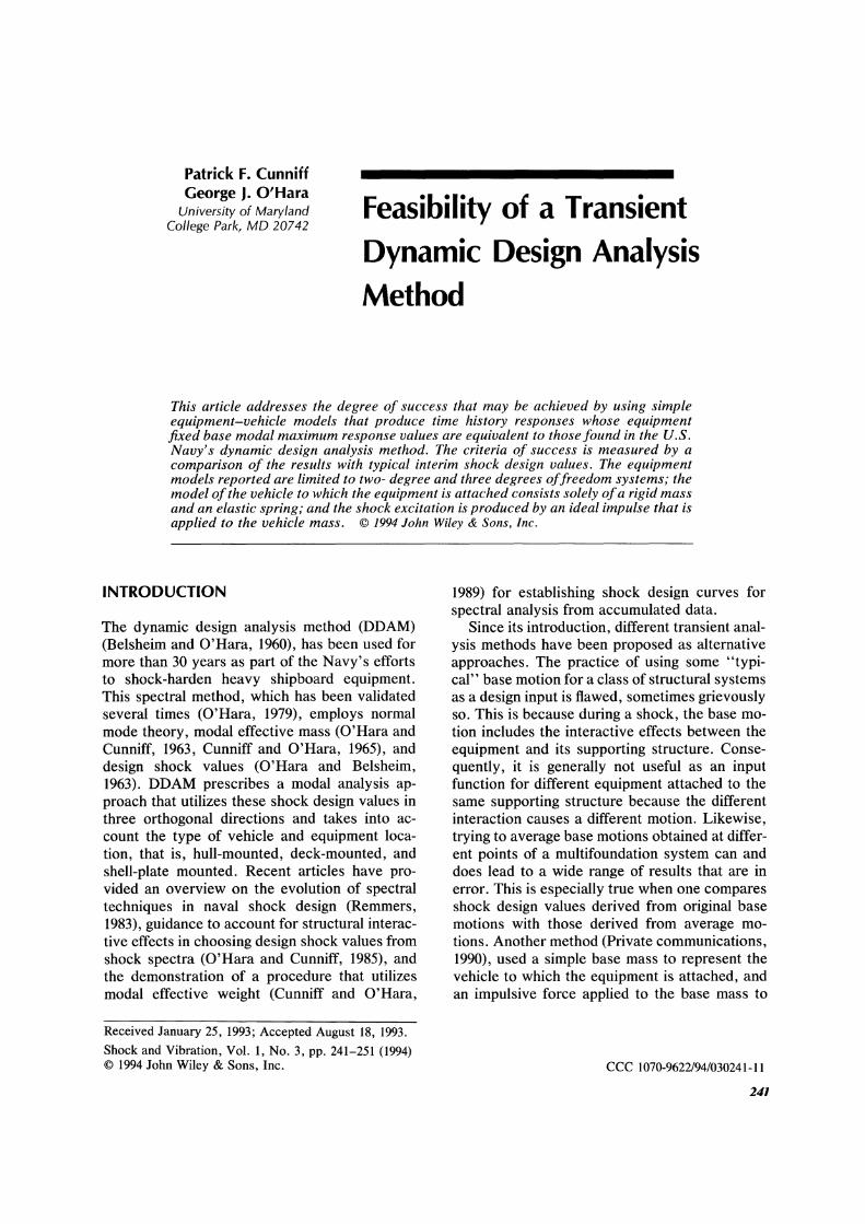
Consider the equipment attached to the vehicle in Fig. l(a) that is subject to a shock excitation. The equipment may be replaced by a dynamically equivalent modal model composed of its normal mode oscillators as shown in Fig. l(b), where dynamical equivalence is defined as the response of the vehicle and the equipment-vehicle boundary being identical for the systems in Fig. l(a, b). The mass of each oscillator is called the modal effective mass and the frequency of
(8) (b)
FIGURE 1 Equipment modeled by its modal oscillators.
---.. en
150
125
100
~ 75
Z 50
25 /" ~'
F'
/ /
/ /
/
21tV 9
/-------------------
/ -- --- ----- --- -- -- ----------------- -- ---------//,'
/,' //
/,' /,' -- W = 20 kips
- - - W = 40 kips ------ W = 60 kips
04Trnn<Tnn<Tn~Tn~Tn~rn~rn~TOn o 25 50 75 100125150175200
Frequency (Hz)
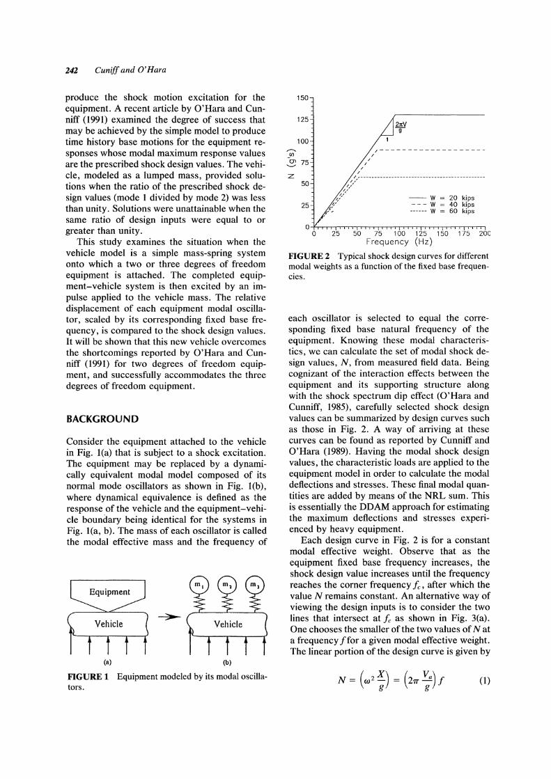
FIGURE 2 Typical shock design curves for different modal weights as a function of the fixed base frequencies.
each oscillator is selected to equal the corresponding fixed base natural frequency of the equipment. Knowing these modal characteristics, we can calculate the set of modal shock design values, N, from measured field data. Being cognizant of the interaction effects between the equipment and its supporting structure along with the shock spectrum dip effect (O'Hara and Cunniff, 1985), carefully selected shock design values can be summarized by design curves such as those in Fig. 2. A way of arriving at these curves can be found as reported by Cunniff and O'Hara (1989). Having the modal shock design values, the characteristic loads are applied to the equipment model in order to calculate the modal deflections and stresses. These final modal quantities are added by means of the NRL sum. This is essentially the DDAM approach for estimating the maximum deflections and stresses experienced by heavy equipment.
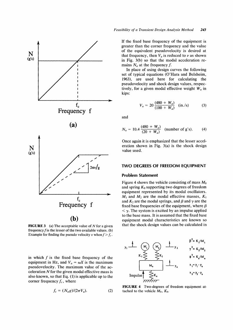
Each design curve in Fig. 2 is for a constant modal effective weight. Observe that as the equipment fixed base frequency increases, the shock design value increases until the frequency reaches the corner frequency Ie, after which the value N remains constant. An alternative way of viewing the design inputs is to consider the two lines that intersect at Ie as shown in Fig. 3(a). One chooses the smaller of the two values of Nat a frequency I for a given modal effective weight. The linear portion of the design curve is given by
(1)
N (g'S)
N (g's)
fc Frequency f
(a)
fc Frequency f
(b) FIGURE 3 (a) The acceptable value of N for a given frequency fis the lesser of the two available values. (b) Example for finding the pseudo velocity v whenf> fe.
in which J is the fixed base frequency of the equipment in Hz, and Va = wX is the maximum pseudovelocity. The maximum value of the acceleration N for the given modal effective mass is also known, so that Eq. (1) is applicable up to the comer frequency!c, where
(2)
Feasibility of a Transient Design Analysis Method 243
If the fixed base frequency of the equipment is greater than the comer frequency and the value of the equivalent pseudovelocity is desired at that frequency, then Va is reduced to 1) as shown in Fig. 3(b) so that the modal acceleration remains N a at the frequency J.
In place of using design curves the following set of typical equations (O'Hara and Belsheim, 1963), are used here for calculating the pseudovelocity and shock design values, respectively, for a given modal effective weight Wa in kips:
v = 20 (480 + Wa) (in./s) a (100 + Wa)
(3)
and
(480 + Wa) ( , Na = lOA (20 + Wa) number of g s). (4)
Once again it is emphasized that the lesser acceleration shown in Fig. 3(a) is the shock design value used.
TWO DEGREES OF FREEDOM EQUIPMENT
Problem Statement
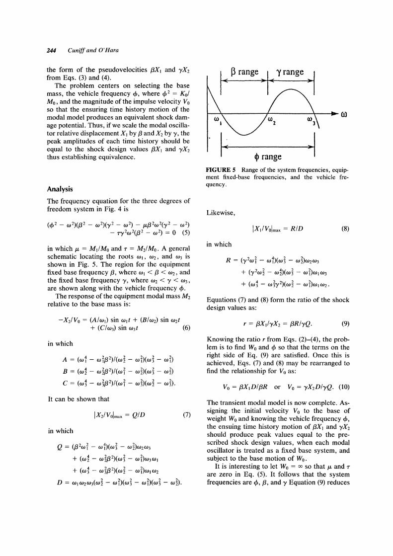
Figure 4 shows the vehicle consisting of mass Mo and spring Ko supporting two degrees of freedom equipment represented by its modal oscillators. MJ and M2 are the modal effective masses, KJ and K2 are the modal springs, and f3 and 'Yare the fixed base frequencies of the equipment, where f3 < 'Y. The system is excited by an impulse applied to the base mass. It is assumed that the fixed base equipment modal characteristics are known so that the shock design values can be calculated in
2 P '" K/MI
2 Y '" KiM2
~Yl 41 2", K 1M
Q Q
FIGURE 4 Two-degrees of freedom equipment attached to the vehicle Mo, Ko.
244 Cuniff and O'Hara
the form of the pseudovelocities f3XI and yXI from Eqs. (3) and (4).
The problem centers on selecting the base mass, the vehicle frequency <p, where <p2 = Ko/ Mo, and the magnitude of the impulse velocity Vo so that the ensuring time history motion of the modal model produces an equivalent shock damage potential. Thus, if we scale the modal oscillator relative displacement XI by f3 and X 2 by y, the peak amplitudes of each time history should be equal to the shock design values f3X I and yX2 thus establishing equivalence.
Analysis
The frequency equation for the three degrees of freedom system in Fig. 4 is
(<p2 - (2)(f32 - (2)(y2 - ( 2) - JLf32W2(y2 - ( 2) - ry 2w 2(f32 - ( 2) = 0 (5)
in which JL = MI/Mo and T = M2/Mo. A general schematic locating the roots WI, W2, and W3 is shown in Fig. 5. The region for the equipment fixed base frequency f3, where WI < f3 < wz, and the fixed base frequency y, where W2 < Y < W3, are shown along with the vehicle frequency <p.
The response of the equipment modal mass M2 relative to the base mass is:
-X2/VO = (A/wI) sin Wit + (B/W2) sin w2t + (C/W3) sin W3t (6)
in which
A = (wi - wif32)/(W~ - wi)(w~ - wi)
B = (wi - w~f32)/(wi - w~)(wj - w~)
C = (w1 - w~f32)/(wi - w~)(w~ - w~).
It can be shown that
in which
Q = (f3 2wi - wi)(wj - W~)W2W3
+ (wi - w~f32)(W~ - Wr)W3WI
+ (w~ - w~f32)(W~ - wr)wI W2
D = WI W2W3(W~ - wi)(w~ - wr)(w~ - w~).
I_ ~ range ~I_ yrange ~I
r-~--------~--------~--~ro
I~ cp range
FIGURE 5 Range of the system frequencies, equipment fixed-base frequencies, and the vehicle frequency.
Likewise,
in which
R = (yIwi - wi)(w~ - W~)W2W3
+ (y2w~ - wi)(w~ - wr)wI W3
+ (w~ - wh2)(w~ - Wi)Wl WI.
(8)
Equations (7) and (8) form the ratio of the shock design values as:
(9)
Knowing the ratio r from Eqs. (2)-(4), the problem is to find Wo and <p so that the terms on the right side of Eq. (9) are satisfied. Once this is achieved, Eqs. (7) and (8) may be rearranged to find the relationship for Vo as:
The transient modal model is now complete. Assigning the initial velocity Vo to the base of weight Wo and knowing the vehicle frequency <p, the ensuing time history motion of f3X1 and yX2 should produce peak values equal to the prescribed shock design values, when each modal oscillator is treated as a fixed base system, and subject to the base motion of Wo.
It is interesting to let Wo = 00 so that JL and T
are zero in Eq. (5). It follows that the system frequencies are <p, f3, and y Equation (9) reduces
Feasibility of a Transient Design Analysis Method 245
to
r = ~(y - cp)/[y(B - cp)] (11)
from which cp is found:
cp = ~ (1 - r)
(~ - r)' (12)
Because cp must be positive and ~ < y, there is a gap where Eq. (12) holds, namely, ~/y < r < 1. It was observed that for the limited number of examples studied to date, the values of cp less than cp in Eq. (12) could never yield a transient model that satisfies its DDAM design ratio r.
Finally, if we let Wo approach zero in Eq. (9), it reduces to
r = ~/y. (13)
Example 1
Let the modal effective weights for the two degrees offreedom equipment in Fig. 4be 26 and 60 kips and the corresponding fixed base frequencies equal 27 and 61 Hz, respectively. The shock design values, obtained from Eqs. (2)-(4) are the pseudovelocities ~Xl = 80.31746 in.!s and yX2 = 67.50000 in.!s) so that the ratio r = 1.1899. Note
Table 1. Example 1
Reference /3X. = Reference yX2 = 67.5000 80.3175 in.ls in.ls
cf> Wo Vo Design (Hz) (kips) (in.ls) I/3Xtlmax lyX21max
27 79.44 67.9910 79.0696 66.1933 69.0641 80.3175 67.2380
2 13.5 251.40 60.1793 79.9947 67.4454 60.2280 80.0594 67.5000
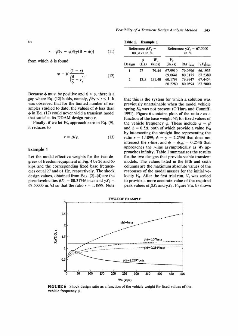
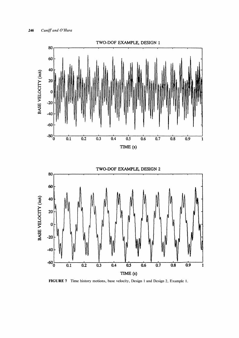
that this is the system for which a solution was previously unattainable when the model vehicle spring Ko was not present (O'Hara and Cunniff, 1991). Figure 6 contains plots of the ratio r as a function of the base weight Wo for fixed values of the vehicle frequency cpo These include cp = ~ and cp = 0.5~, both of which provide a value Wo by intersecting the straight line representing the ratio r = 1.1899; cp = y = 2.259~ that does not intersect the r-line; and cp = CPmin = 0.254~ that approaches the r-line asymptotically as Wo approaches infinity. Table 1 summarizes the results for the two designs that provide viable transient models. The values listed in the fifth and sixth columns are the maximum absolute values of the responses of the modal masses for the initial velocity Vo. After the first trial run, Vo was scaled to provide a more accurate value of the required peak values of ~Xl and yX2 • Figure 7(a, b) shows
TWO·DOF EXAMPLE
..
3r---~--~----~--~--~----r---~--~----r---.
2.S
2
--" " ,-
phi-beta _--------,..-"
-' --..-,,-
-----' ,---_ ..
" ,-",,,,, phi-O.s·beta " _.-._._._._._._._._._._._._._._._.-
°O~--~SO~~1~OO~~1~SO~-=200=-~~~O~~300=-~3~S~O--~~~--7.~~O--~SOO
Wo (kips)
FIGURE 6 Shock design ratio as a function of the vehicle weight for fixed values of the vehicle frequency cf>.
246 Cuniff and O'Hara
80
60
-. 40 .se. .5 '-'
>- 20 f-o 0 9 0 tIJ > -20 tIl
~ (Xl -40
-60
-80 0 0.1 0.2
80
60
-.se. 40 .5 '-'
>< f-o 20 -U
9 tIJ 0 > tIJ
~ -20 (Xl
~
-40
-60 0 0.1 0.2
TWO-DOF EXAMPLE, DESIGN 1
0.3 0.4 0.5 0.6 0.7
TIME (s)
TWO-OOF EXAMPLE, DESIGN 2
0.3 0.4
~
0.5
TIME (s)
~ ~
0.6 0.1
0.8 0.9
~
~
0.8 0.9
FIGURE 7 Time history motions, base velocity, Design 1 and Design 2, Example 1.
1
1
----Ul
4000
'2-3000 '---'
~ ] 2000 Q. (j)
.::£ g 1000
..c (j)
-- Design 1 ------- Design 2
:i " " " :1,
fl. f2 = fixed base frequencies
.. / \ ----------------------0~0~~;20~~;4~OrT~6~0~.-8'0~~10iO~~120
Frequency (Hz)
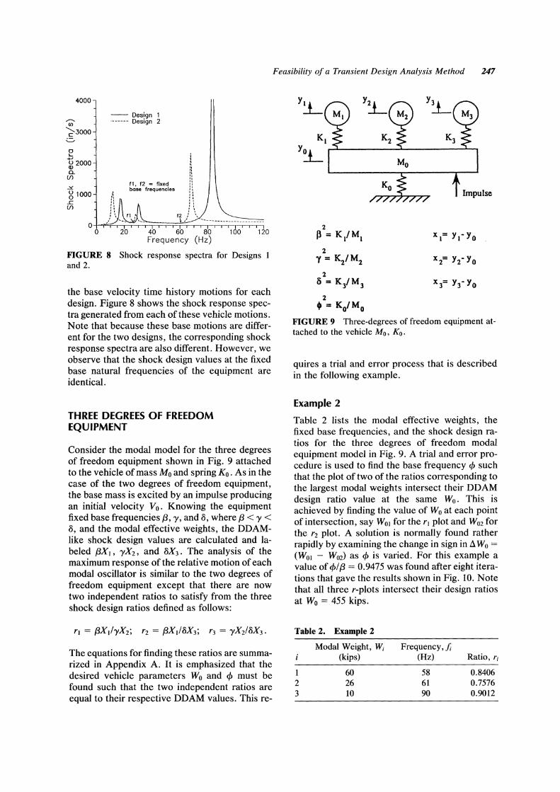
FIGURE 8 Shock response spectra for Designs 1 and 2.
the base velocity time history motions for each design_ Figure 8 shows the shock response spectra generated from each of these vehicle motions. Note that because these base motions are different for the two designs, the corresponding shock response spectra are also different. However, we observe that the shock design values at the fixed base natural frequencies of the equipment are identical.
THREE DEGREES OF FREEDOM EQUIPMENT
Consider the modal model for the three degrees of freedom equipment shown in Fig. 9 attached to the vehicle of mass Mo and spring Ko. As in the case of the two degrees of freedom equipment, the base mass is excited by an impulse producing an initial velocity Vo. Knowing the equipment fixed base frequencies {3, 1', and 8, where {3 < l' < 8, and the modal effective weights, the DDAMlike shock design values are calculated and labeled (3Xl' 'YX2, and 8X3 • The analysis of the maximum response ofthe relative motion of each modal oscillator is similar to the two degrees of freedom equipment except that there are now two independent ratios to satisfy from the three shock design ratios defined as follows:
The equations for finding these ratios are summarized in Appendix A. It is emphasized that the desired vehicle parameters Wo and <P must be found such that the two independent ratios are equal to their respective DDAM values. This re-
Feasibility of a Transient Design Analysis Method 247
Kl Y ~ ,.:L-----1.------'-1
2 11 = K/Ml
2 Y = K2/M2
2 S = KiM)
2 • = KoiMo
FIGURE 9 Three-degrees of freedom equipment attached to the vehicle Mo, Ko.
quires a trial and error process that is described in the following example.
Example 2
Table 2 lists the modal effective weights, the fixed base frequencies, and the shock design ratios for the three degrees of freedom modal equipment model in Fig. 9. A trial and error procedure is used to find the base frequency <p such that the plot of two of the ratios corresponding to the largest modal weights intersect their DDAM design ratio value at the same Wo. This is achieved by finding the value of Wo at each point of intersection, say WOl for the rl plot and W02 for the r2 plot. A solution is normally found rather rapidly by examining the change in sign in Ll Wo =
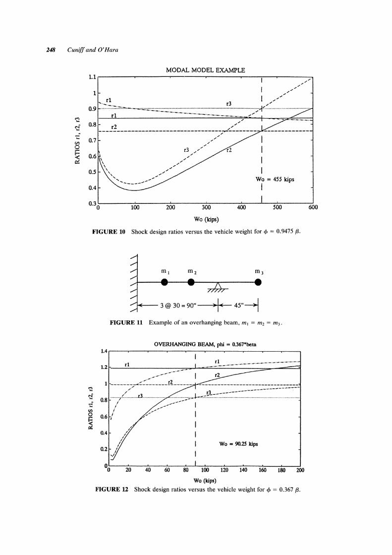
(WOl - W02) as <p is varied. For this example a value of <PI {3 = 0.9475 was found after eight iterations that gave the results shown in Fig. 10. Note that all three r-plots intersect their design ratios at Wo = 455 kips.
Table 2. Example 2
Modal Weight, Wi (kips)
1 60 2 26 3 10
Frequency, fi (Hz) Ratio, ri
58 0.8406 61 0.7576 90 0.9012
248 Cuniff and O'Hara
M ... r-i ... -i:
en 0
~ 0::
MODAL MODEL EXA.\1PLE 1.1.-------~------~--------~------~--_.1--~------~"
./' " 1 I ~///
.... _r: r3 I /// 0.9 ......... ~~;"':"'.-.-.-''''::::;:::::::::::::::::::::::::::::::::::~:~:~:~:~:~:~:~:~:~:~: .... ~.;.;."'~ ...................................... .
0.8
0.7
0.5
0.4
r2 /// " "
-----------------------------------~--------
J"///
~~
-----."..-
..-./ .,. ./
r3 ./,,"
" ./
./
,,/
" " ,," I I I I
Wo = 455 kips
I
Q30~-------1~OO~----~2~OO~----~3~OO~----~400~--~--~5700~----~600
Wo (kips)
FIGURE 10 Shock design ratios versus the vehicle weight for cjJ = 0.9475 f3.
...... ... CIl o ~ a:
~--- 3@30= 90" --~"~I"""<- 45"--1
FIGURE 11 Example of an overhanging beam, m) = m2 = m3.
OVERHANGING BEAM, phi = O.367·beta 1.4 r---,----.------.----.------.----.-----.----.-----..,.-----.
r1 _._._.~1:...-. 1.2 r---.:.=..------------_-:.--:::.-~ . ....1--==:.:=.=-----------::::::=o_--====~ _._._._.-.- -- - _._._.
-.~.-
1 -------~~:~-----!~------ ---____________________________ _ .' -----------........ ;/< ....... r3. ..................................... :;;=-.".l.~".".?~.:-:.:-:~.~.~.~.~~.~.~.~.~~.~~.~~ ................................ .
0.8 .I _----- I ! ,,-
I _-
0.6 / ",-- I I
0.4 I
0.2 Wo = 90.25 kips
°0~--~2~0--~4~0--~OO~--8=O~~1~OO~~1~20~~14~0---7100~--1~8~O--~200
Wo (kips)
FIGURE 12 Shock design ratios versus the vehicle weight for cjJ = 0.367 f3.
Feasibility of a Transient Design Analysis Method 249
OVERHANGING BEAM l00r---~----r---~--~----~--~--~----~---r---'
80
60
40
20
>< 0 :.: til -20 CD
a
b
c
-40
-60
-80
-1000 0.1 0.2 o.s 0.6 0.7
TIME 1(1)
60
40
o
·20
-40
·800L----o.~I----O'~2---~O.~1~-O~.4~~0'~S--~O'~6---0~.7----0~.8~~O'~9~~ TIMEICI)
80
60
·40
·60
1111111 1111111
·80
.1000~--~o.~1--~o.~2---0~.l~~O~.4--~O~.S--~0.-6---o.~7----0~.8----0~.9~~ TIME 1(1)
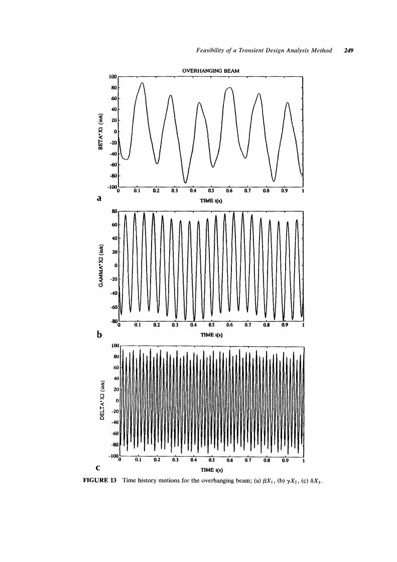
FIGURE 13 Time history motions for the overhanging beam; (a) f3X\, (b) -yX2' (c) ax3 •
250 Cuniff and O'Hara
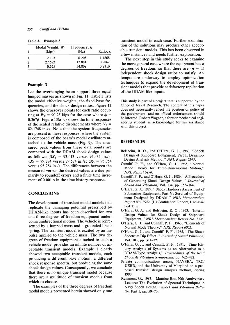
Table 3. Example 3
1 2 3
Modal Weight, Wi (kips)
2.103 27.572 0.325
Example 3
Frequency, fi (Hz)
6.205 17.884 54.808
Ratio, ri
1.1868 0.9862 0.8310
Let the overhanging beam support three equal lumped masses as shown in Fig. 11. Table 3 lists the modal effective weights, the fixed base frequencies, and the shock design ratios. Figure 12 shows the crossover points for each ratio occurring at Wo = 90.25 kips for the case where cP =
0.367{3. Figure 13(a-c) shows the time responses of the scaled relative displacements where Vo =
82.1748 in.! s. Note that the system frequencies are present in these responses, where the system is composed of the beam's modal oscillators attached to the vehicle mass (Fig. 9). The measured peak values from these data points are compared with the DDAM shock design values as follows: {3XJ = 93.013 versus 94.435 in./s; yXz = 79.374 versus 79.574 in.!s; 8X3 = 95.754 versus 95.754 in.!s. The differences between the measured versus the desired values are due primarily to roundoff errors and a finite time increment of 0.001 s in the time history response.
CONCLUSIONS
The development of transient modal models that replicate the damaging potential prescribed by DDAM-like inputs has been described for two and three degrees of freedom equipment undergoing unidirectional motion. The vehicle is represented by a lumped mass and a grounded linear spring. The transient model is excited by an impulse applied to the vehicle mass. The two degrees of freedom equipment attached to such a vehicle model provides an infinite number of acceptable transient models. Example 1 clearly showed two acceptable transient models, each producing a different base motion, a different shock response spectra, but producing the same shock design values. Consequently, we conclude that there is no unique transient model because there are a multitude of transient models from which to choose.
The examples of the three degrees of freedom modal models presented herein showed only one
transient model in each case. Further examination of the solutions may produce other acceptable transient models. This has been observed in a few instances and needs further exploration.
The next step in this study seeks to examine the more general case where the equipment has n degrees of freedom, so that there are (n - 1) independent shock design ratios to satisfy. Attempts are underway to employ optimization techniques to expand the development of transient models that provide satisfactory replication of the DDAM-like inputs.
This study is part of a project that is supported by the Office of Naval Research. The content of this paper does not necessarily reflect the position or policy of the government, and no official endorsement should be inferred. Robert Wagner, a former mechanical engineering student, is acknowledged for his assistance with this project.
REFERENCES
Belsheim, R. 0., and O'Hara, G. J., 1960, "Shock Design of Shipboard Equipment, Part I, DynamicDesign Analysis Method," NRL Report 5545.
Cunniff, P. F., and O'Hara, G. J., 1965, "Normal Mode Theory for Three-Dimensional Motion," NRL Report 6170.
Cunniff, P. F., and O'Hara, G. J., 1989, "A Procedure of Generating Shock Design Values," Journal of Sound and Vibration, Vol. 134, pp. 155-164.
O'Hara, G. J., 1979, "Shock Hardness Assessment of Submarine Equipment; Part V; Survival of Equipment Designed by DDAM," NRL Memorandum Report No. 3942, (U) Confidential Report, Unclassified Title.
O'Hara, G. J., and Belsheim, R. 0., 1963, "Interim Design Values for Shock Design of Shipboard Equipment," NRL Memorandum Report No. 1396.
O'Hara, G. J., and Cunniff, P. F., 1963, "Elements of Normal Mode Theory," NRL Report 6002.
O'Hara, G. J., and Cunniff, P. F., 1985, "The Shock Spectrum Dip Effect," Journal of Sound Vibration, Vol. 103, pp. 311-321.
O'Hara, G. J., and Cunniff, P. F., 1991, "Time History Analysis of Systems as an Alternative to a DDAM-Type Analysis," Proceedings of the 62nd Shock & Vibration Symposium, pp. 462-472.
Private communications among NA VSEA, TRCI UERD, and the University of Maryland on a proposed transient design analysis method, Spring 1990.
Remmers, G., 1983, "Maurice Biot 50th Anniversary Lecture: The Evolution of Spectral Techniques in Navy Shock Design," Shock and Vibration Bulletin, Part I, pp. 59-70.
Feasibility of a Transient Design Analysis Method 251
APPENDIX A
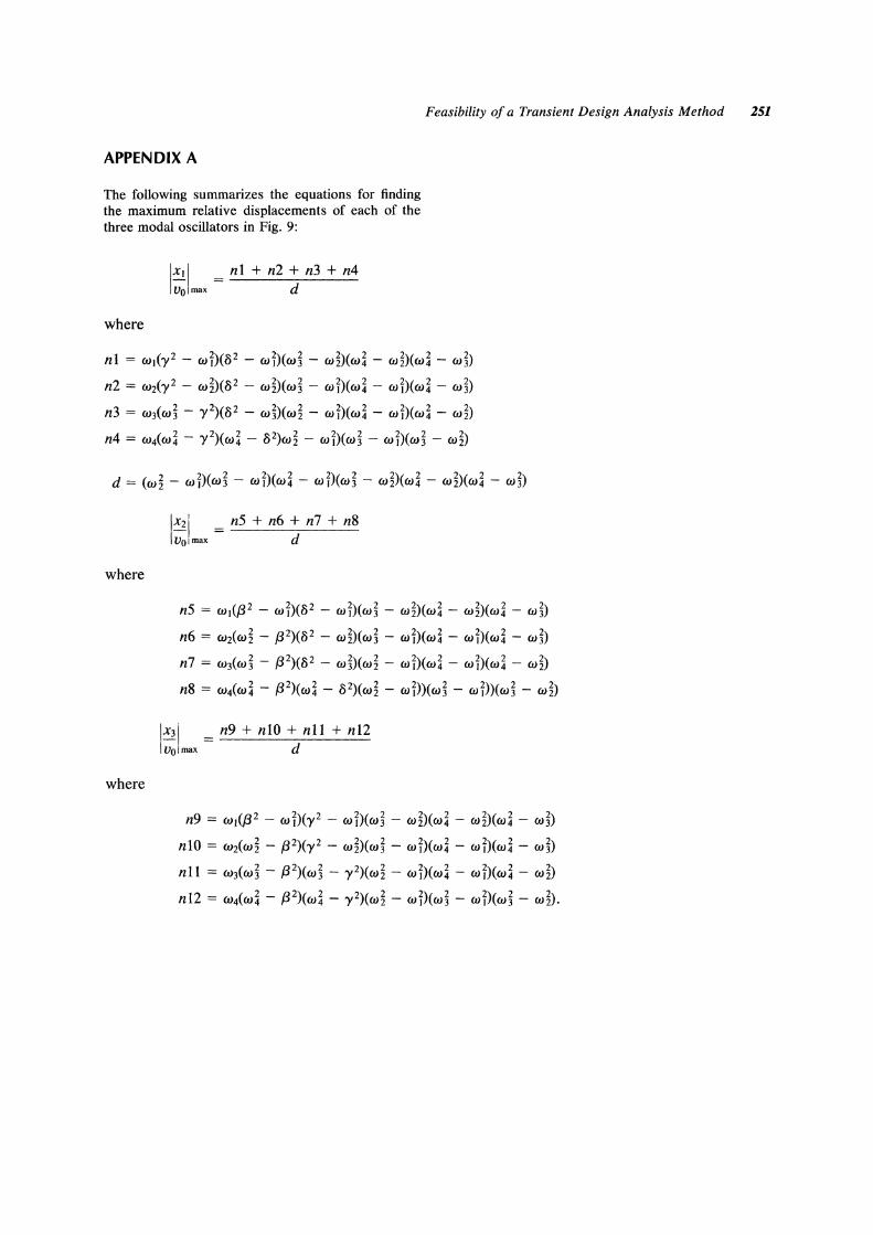
The following summarizes the equations for finding the maximum relative displacements of each of the three modal oscillators in Fig. 9:
IXII = ni + n2 + n3 + n4 vo I max d
where
nl = WI(y2 - w1)(8 2 - w1)(wj - w~)(W~ - w~)(w~ - wj)
n2 = W2(y2 - w~)(82 - w~)(wj - wl)(w~ - wl)(w~ - wj)
n3 = W3(Wj - 1'2)(82 - wj)(W~ - wl)(w~ - wl)(w~ - w~)
n4 = W4(W~ - y2)(W~ - 82)W~ - wl)(wj - wl)(wj - w~)
where
where
1X2i = n5 + n6 + n7 + n8 IVOlmax d
n5 = WI(/Y - wl)(8 2 - wl)(wj - w~)(w~ - w~)(w~ - wj)
n6 = W2(W~ - 13 2)(82 - W~)(wj - wNw~ - wl)Cw~ - wj)
n7 = W3(Wj - 13 2)(8 2 - wj)(W~ - wj)(W~ - wl)(w~ - w~)
n8 = W4CW~ - f32)(W~ - 82)(W~ - Wj))Cwj - wj))Cwj - W~)
IX31 = n9 + nlO + nIl + n12 I vol max d
n9 = WICf3 2 - W1)Cy 2 - wj)Cwj - W~)(W~ - W~)CW~ - W~)
nlO = w2(wi - 13 2)(1'2 - w~)Cwj - wj)Cw~ - wj)(w~ - wj)
nIl = w3Cwj - f32)CW~ - y2)(wi - wj)Cw~ - wj)(w~ - wi)
nI2 = W4(W~ - f32)(W~ - y2)(w~ - wj)(wj - wDcw~ - w~).

International Journal of
AerospaceEngineeringHindawi Publishing Corporationhttp://www.hindawi.com Volume 2010
RoboticsJournal of
Hindawi Publishing Corporationhttp://www.hindawi.com Volume 2014
Hindawi Publishing Corporationhttp://www.hindawi.com Volume 2014
Active and Passive Electronic Components
Control Scienceand Engineering
Journal of
Hindawi Publishing Corporationhttp://www.hindawi.com Volume 2014
International Journal of
RotatingMachinery
Hindawi Publishing Corporationhttp://www.hindawi.com Volume 2014
Hindawi Publishing Corporation http://www.hindawi.com
Journal ofEngineeringVolume 2014
Submit your manuscripts athttp://www.hindawi.com
VLSI Design
Hindawi Publishing Corporationhttp://www.hindawi.com Volume 2014
Hindawi Publishing Corporationhttp://www.hindawi.com Volume 2014
Shock and Vibration
Hindawi Publishing Corporationhttp://www.hindawi.com Volume 2014
Civil EngineeringAdvances in
Acoustics and VibrationAdvances in
Hindawi Publishing Corporationhttp://www.hindawi.com Volume 2014
Hindawi Publishing Corporationhttp://www.hindawi.com Volume 2014
Electrical and Computer Engineering
Journal of
Advances inOptoElectronics
Hindawi Publishing Corporation http://www.hindawi.com
Volume 2014
The Scientific World JournalHindawi Publishing Corporation http://www.hindawi.com Volume 2014
SensorsJournal of
Hindawi Publishing Corporationhttp://www.hindawi.com Volume 2014
Modelling & Simulation in EngineeringHindawi Publishing Corporation http://www.hindawi.com Volume 2014
Hindawi Publishing Corporationhttp://www.hindawi.com Volume 2014
Chemical EngineeringInternational Journal of Antennas and
Propagation
International Journal of
Hindawi Publishing Corporationhttp://www.hindawi.com Volume 2014
Hindawi Publishing Corporationhttp://www.hindawi.com Volume 2014
Navigation and Observation
International Journal of
Hindawi Publishing Corporationhttp://www.hindawi.com Volume 2014
DistributedSensor Networks
International Journal of