Pattern-avoiding access in binary search trees

Parinya Chalermsook1, Mayank Goswami1, Laszlo Kozma2, Kurt Mehlhorn1, andThatchaphol Saranurak∗3

1Max-Planck Institute for Informatics, Germany. parinya,gmayank,mehlhorn@mpi-inf.mpg.de

2Saarland University, Germany. kozma@cs.uni-saarland.de

3KTH Royal Institute of Technology, Sweden. thasar@kth.se

Abstract

The dynamic optimality conjecture is perhaps the most fundamental open question about binarysearch trees (BST). It postulates the existence of an asymptotically optimal online BST, i.e. one that isconstant factor competitive with any BST on any input access sequence. The two main candidates fordynamic optimality in the literature are splay trees [Sleator and Tarjan, 1985], and Greedy [Lucas, 1988;Munro, 2000; Demaine et al. 2009]. Despite BSTs being among the simplest data structures in computerscience, and despite extensive effort over the past three decades, the conjecture remains elusive. Dynamicoptimality is trivial for almost all sequences: the optimum access cost of most length-n sequences isΘ(n logn), achievable by any balanced BST. Thus, the obvious missing step towards the conjecture isan understanding of the “easy” access sequences, and indeed the most fruitful research direction so farhas been the study of specific sequences, whose “easiness” is captured by a parameter of interest. Forinstance, splay provably achieves the bound of O(nd) when d roughly measures the distances betweenconsecutive accesses (dynamic finger), the average entropy (static optimality), or the delays betweenmultiple accesses of an element (working set). The difficulty of proving dynamic optimality is witnessedby other highly restricted special cases that remain unresolved; one prominent example is the traversalconjecture [Sleator and Tarjan, 1985], which states that preorder sequences (whose optimum is linear) arelinear-time accessed by splay trees; no online BST is known to satisfy this conjecture.

In this paper, we prove two different relaxations of the traversal conjecture for Greedy: (i) Greedyis almost linear for preorder traversal, (ii) if a linear-time preprocessing1 is allowed, Greedy is in factlinear. These statements are corollaries of our more general results that express the complexity of accesssequences in terms of a pattern avoidance parameter k. Pattern avoidance is a well-established conceptin combinatorics, and the classes of input sequences thus defined are rich, e.g. the k = 3 case includespreorder sequences. For any sequence X with parameter k, our most general result shows that Greedy

achieves the cost n2α(n)O(k)

where α is the inverse Ackermann function. Furthermore, a broad subclassof parameter-k sequences has a natural combinatorial interpretation as k-decomposable sequences. For

this class of inputs, we obtain an n2O(k2) bound for Greedy when preprocessing is allowed. For k = 3,these results imply (i) and (ii). To our knowledge, these are the first upper bounds for Greedy thatare not known to hold for any other online BST. To obtain these results we identify an input-revealingproperty of Greedy. Informally, this means that the execution log partially reveals the structure of theaccess sequence. This property facilitates the use of rich technical tools from forbidden submatrix theory.

Further studying the intrinsic complexity of k-decomposable sequences, we make several observations.First, in order to obtain an offline optimal BST, it is enough to bound Greedy on non-decomposableaccess sequences. Furthermore, we show that the optimal cost for k-decomposable sequences is Θ(n log k),which is well below the proven performance of all known BST algorithms. Hence, sequences in this classcan be seen as a “candidate counterexample” to dynamic optimality.

∗Work partly done while at Saarland University.1The purpose of preprocessing is to bring the data structure into a state of our choice. This state is independent of the

actual input. This kind of preprocessing is implicit in the Demaine et al. definition of Greedy.

i

1 Introduction

The binary search tree (BST) model is one of the most fundamental and thoroughly studied data accessmodels in computer science. In this model, given a sequence X ∈ [n]m of keys, we are interested in OPT(X),the optimum cost of accessing X by a binary search tree. When the tree does not change between accesses,OPT is well understood: both efficient exact algorithms (Knuth [23]) and a linear time approximation(Mehlhorn [28]) have long been known. By contrast, in the dynamic BST model (where restructuring of thetree is allowed between accesses) our understanding of OPT is very limited. No polynomial time exact orconstant-approximation algorithms are known for computing OPT in the dynamic BST model.

Theoretical interest in the dynamic BST model is partly due to the fact that it holds the possibilityof a meaningful “instance optimality”, i.e. of a BST algorithm that is constant factor competitive (in theamortized sense) with any other BST algorithm, even with those that are allowed to see into the future. Theexistence of such a “dynamically optimal” algorithm has been postulated in 1985 by Sleator and Tarjan [34];they conjectured their splay tree to have this property. Later, Lucas [25] and independently Munro [29]proposed a greedy offline algorithm as another candidate for dynamic optimality. In 2009 Demaine, Harmon,Iacono, Kane, and Patrascu (DHIKP) [11] presented a geometric view of the BST model, in which the Lucas-Munro offline algorithm naturally turns into an online one (simply called Greedy). Both splay and Greedyare considered plausible candidates for achieving optimality. However, despite decades of research, neither ofthe two algorithms are known to be o(log n)-competitive (the best known approximation ratio for any BSTis O(log log n) [12], but the algorithms achieving this bound are less natural). Thus, the dynamic optimalityconjecture remains wide open.

Why is dynamic optimality difficult to prove (or disprove)? For a vast majority of access sequences,the optimal access cost by any dynamic BST (online or offline) is2 Θ(m log n) and any static balanced treecan achieve this bound.3 Hence, dynamic optimality is almost trivial on most sequences. However, when aninput sequence has complexity o(m log n), a candidate BST must “learn” and “exploit” the specific structureof the sequence, in order to match the optimum. This observation motivates the popular research directionthat aims at understanding “easy” sequences, i.e. those with OPT = O(md) when d is a parameter thatdepends on the structure of the sequence; typically d = o(log n). Parameter d can be seen as a measure of“easiness”, and the objective is to prove that a candidate algorithm achieves the absolute bound of O(md);note that this does not immediately imply that the algorithm matches the optimum.

The splay tree is known to perform very well on many “easy” sequences: It achieves the access time ofO(md) when d is a parameter that roughly captures the average distances between consecutive accesses [9,10],the average entropy, or the recentness of the previous accesses [34]; these properties are called dynamicfinger, static optimality and working set bounds respectively (the latter two bounds are also satisfied byGreedy [15]). The notorious difficulty of dynamic optimality is perhaps witnessed by the fact that manyother highly restricted special cases have resisted attempts and remain unresolved. These special cases standas a roadblock to proving (or disproving) the optimality of any algorithm: proving that A is optimal requiresproving that it performs well on the easy inputs; refuting the optimality of A requires a special “easy”subclass on which A is provably inefficient. In any case, a better understanding of easy sequences is needed,but currently lacking, as observed by several authors [11,30].

One famous example of such roadblocks is the traversal conjecture, proposed by Sleator and Tarjan in1985. This conjecture states that starting with an arbitrary tree T (called initial tree) and accessing its keysusing the splay algorithm in the order given by the preorder sequence of another tree T ′ takes linear time.Since the optimum of such preorder sequences is linear, any dynamically optimal algorithm must match thisbound. After three decades, only very special cases of this conjecture are known to hold, namely when T ′

is a monotone path (the so-called sequential access [36]) or when T ′ = T [8].4 Prior to this work, no onlineBST algorithm was known to be linear on such access sequences.

Motivated by well-established concepts in combinatorics [21, 24, 37], in this paper we initiate the studyof the complexity of access sequences in terms of pattern avoidance parameters. Our main contributions are

2This observation appears to be folklore. We include a proof in Appendix G.3As customary, we only consider successful accesses, we ignore inserts and deletes, and we assume that m ≥ n.4This result implies an offline BST with O(n) cost for accessing a preorder sequence, by first rotating T to T ′.

1

Structure splay bound Greedy bound Remark

Staticoptimality

low entropy O(∑ni=1 fi(1 + log m

fi))

[34]

same as splay [6, 15] corollaries ofAccess Lemma[34]Working set temporal locality O(m+ n logn+

∑mt=1 log(τt + 1))

[34]same as splay [6, 15]

Dynamicfinger

key-space locality O(m+∑mt=2 log |xt − xt−1|)

[9, 10]?

Deque n updates at min/maxelements

O(nα∗(n)) [30] O(n2α(n)) [7] O(n) formulti-splay [38] from

empty treeSequential avoid (2, 1) O(n) [31,36] O(n) [7, 15]

Traversal avoid (2, 3, 1) ? n2α(n)O(1)[* Cor 1.2] OPT = O(n)

Pattern-avoiding(new)

avoid (2, 3, 1) withpreprocessing

? O(n) [* Cor 1.5] OPT = O(n)

avoid (k, . . . , 1)(k-increasing)

? n2O(k2) [* Thm 1.6]

avoid all simple perm. ofsize > k (k-decomposable)with preprocessing

? n2O(k2) [* Thm 1.4] OPT = O(n log k)[* Cor 1.10]

avoid an arbitrary perm.of size k

? n2α(n)O(k)[* Thm 1.1] Best known lower

bound is at mostn2O(k) [* Thm 1.7]

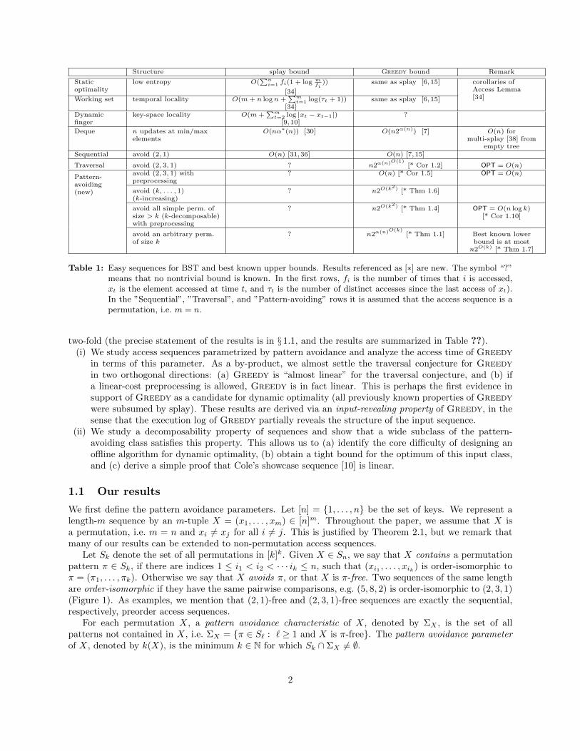
Table 1: Easy sequences for BST and best known upper bounds. Results referenced as [∗] are new. The symbol “?”means that no nontrivial bound is known. In the first rows, fi is the number of times that i is accessed,xt is the element accessed at time t, and τt is the number of distinct accesses since the last access of xt).In the ”Sequential”, ”Traversal”, and ”Pattern-avoiding” rows it is assumed that the access sequence is apermutation, i.e. m = n.

two-fold (the precise statement of the results is in § 1.1, and the results are summarized in Table ??).(i) We study access sequences parametrized by pattern avoidance and analyze the access time of Greedy

in terms of this parameter. As a by-product, we almost settle the traversal conjecture for Greedyin two orthogonal directions: (a) Greedy is “almost linear” for the traversal conjecture, and (b) ifa linear-cost preprocessing is allowed, Greedy is in fact linear. This is perhaps the first evidence insupport of Greedy as a candidate for dynamic optimality (all previously known properties of Greedywere subsumed by splay). These results are derived via an input-revealing property of Greedy, in thesense that the execution log of Greedy partially reveals the structure of the input sequence.

(ii) We study a decomposability property of sequences and show that a wide subclass of the pattern-avoiding class satisfies this property. This allows us to (a) identify the core difficulty of designing anoffline algorithm for dynamic optimality, (b) obtain a tight bound for the optimum of this input class,and (c) derive a simple proof that Cole’s showcase sequence [10] is linear.

1.1 Our results

We first define the pattern avoidance parameters. Let [n] = 1, . . . , n be the set of keys. We represent alength-m sequence by an m-tuple X = (x1, . . . , xm) ∈ [n]m. Throughout the paper, we assume that X isa permutation, i.e. m = n and xi 6= xj for all i 6= j. This is justified by Theorem 2.1, but we remark thatmany of our results can be extended to non-permutation access sequences.

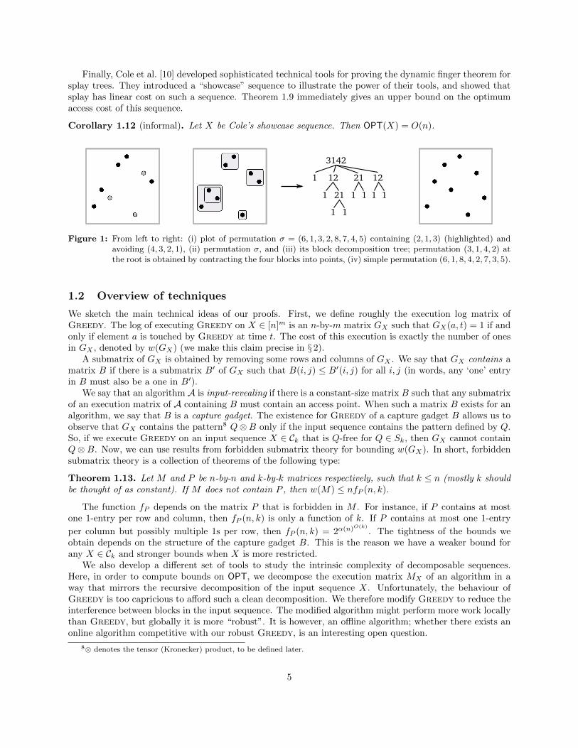
Let Sk denote the set of all permutations in [k]k. Given X ∈ Sn, we say that X contains a permutationpattern π ∈ Sk, if there are indices 1 ≤ i1 < i2 < · · · ik ≤ n, such that (xi1 , . . . , xik) is order-isomorphic toπ = (π1, . . . , πk). Otherwise we say that X avoids π, or that X is π-free. Two sequences of the same lengthare order-isomorphic if they have the same pairwise comparisons, e.g. (5, 8, 2) is order-isomorphic to (2, 3, 1)(Figure 1). As examples, we mention that (2, 1)-free and (2, 3, 1)-free sequences are exactly the sequential,respectively, preorder access sequences.

For each permutation X, a pattern avoidance characteristic of X, denoted by ΣX , is the set of allpatterns not contained in X, i.e. ΣX = π ∈ S` : ` ≥ 1 and X is π-free. The pattern avoidance parameterof X, denoted by k(X), is the minimum k ∈ N for which Sk ∩ ΣX 6= ∅.

2

For each k ∈ N, the pattern avoidance class Ck contains all sequences X with pattern avoidance parameterk. This characterization is powerful and universal: Ci ⊆ Ci+1 for all i, and Cn+1 contains all sequences.

Bounds for Greedy in terms of k. We study the access cost of Greedy in terms of the pattern

avoidance parameter. Our most general upper bound of n2α(n)O(k)

holds for any access sequence in Ck(Theorem 1.1). Later, we show a stronger bound of n2O(k2) for two broad subclasses of Ck that have intuitivegeometric interpretation: k-decomposable sequences (Theorem 1.4), which generalize preorder sequences andk-increasing sequences (Theorem 1.6), which generalize sequential access.

Theorem 1.1. Let X ∈ Ck be an access sequence of length n. The cost of accessing X using Greedy is at

most n2α(n)O(k)

.

The following corollary simply follows from the fact that all preorder sequences X belong to C3 (pluggingk = 3 into the theorem).

Corollary 1.2 (“Almost” traversal conjecture for Greedy). The cost of accessing a preorder sequence of

length n using Greedy, with arbitrary initial tree is at most n2α(n)O(1)

.

Next, we show sharper bounds for Greedy when some structural property of ΣX is assumed. First, weprove a bound when ΣX contains all “non-decomposable” permutations of length at least k + 1. We showthat this property leads to a decomposition that has intuitive geometric meaning, which we describe below.

Given a permutation σ = (σ1, . . . , σ`) ∈ S` we call a set [a, b] a block of σ, if σa, σa+1, . . . , σb =c, c+ 1, . . . , d for some integers c, d ∈ [`]. In words, a block corresponds to a contiguous interval that ismapped to a contiguous interval. We say that a permutation σ ∈ S` is decomposable if there is a block of σof size strictly betweeen 1 and `; otherwise, we say that it is non-decomposable (a.k.a. simple5).

We say that an input sequence X is decomposable into k blocks if there exist disjoint [a1, b1], . . . , [ak, bk]such that each [ai, bi] is a block for X and (

⋃i[ai, bi]) ∩ N = [n]. The recursive decomposition complexity of

a sequence X is at most d if one can recursively decompose X into subblocks until singletons are obtained,and each step creates at most d blocks (equivalently we say that X is d-recursively decomposable, or simplyd-decomposable). See Figure 1. It is easy to see that preorder sequences are 2-decomposable.6

The following lemma (proof in Lemma D.1) connects pattern avoidance and recursive decompositioncomplexity of a sequence.

Lemma 1.3. Let X ∈ Sn. Then ΣX contains all simple permutations of length at least k + 1 if and only ifX is k-decomposable.

This lemma implies in particular that if X is k-decomposable, then X ∈ Ck+1 and Theorem 1.1 canbe applied. The following theorem gives a sharper bound, when a preprocessing (independent of X) isperformed. This yields another relaxed version of the traversal conjecture.

Theorem 1.4. Let X be a k-decomposable access sequence. The cost of accessing X using Greedy, with alinear-cost preprocessing, is at most n2O(k2).

Corollary 1.5 (Traversal conjecture for Greedy with preprocessing). The cost of accessing a preordersequence using Greedy, with preprocessing, is linear.

Our preprocessing step is done in the geometric view (explained in § 2) in order to “hide” the initial treeT from Greedy. In the corresponding tree-view, our algorithm preprocesses the initial tree T , turning itinto another tree T ′, independent of X, and then starts accessing the keys in X using the tree-view variantof Greedy (as defined in [11]). We mention that DHIKP [11] define Greedy without initial tree, and thustheir algorithm (implicitly) performs this preprocessing.

5See [3] for a survey of this well-studied concept. The decomposition described here appears in the literature as substitution-decomposition.

6The entire set of 2-decomposable permutations is known as the set of separable permutations [2].

3

As another natural special case, we look at ΣX ⊇ (k, . . . , 1), for some value k. In words, X hasno decreasing subsequence of length k (alternatively, X can be partitioned into at most k − 1 increasingsubsequences7). Observe that the k = 2 case corresponds to sequential access. We call this the k-increasingproperty of X. Similarly, if ΣX ⊇ (1, . . . , k), we say that X is k-decreasing. We obtain the followinggeneralization of the sequential access theorem (this result holds for arbitrary initial tree).

Theorem 1.6. Let X be a k-increasing or k-decreasing sequence. The cost of accessing X using Greedyis at most n2O(k2).

All the aforementioned results are obtained via the input-revealing property of Greedy (the ideas aresketched in § 1.2).

Bound for signed Greedy in terms of k. We further show the applicability of the input-revealingtechnique. Signed Greedy [11] (denoted SGreedy) is an algorithm similar to Greedy. It does not alwaysproduce a feasible BST solution, but its cost serves as a lower bound for the optimum. Let us denote byA(X) and OPT(X) the cost of an algorithm A on X, respectively the optimum cost of X. Then we haveA(X) ≥ OPT(X), and OPT(X) = Ω(SGreedy(X)).

Conjecture 1 (Wilber [39], using [11]). OPT(X) = Θ(SGreedy(X)) for all input sequences X.

We show that our techniques can be used to upper bound the cost of SGreedy.

Theorem 1.7. The cost of SGreedy on an access sequence X ∈ Ck is at most n2O(k).

Corollary 1.8. Let A be an algorithm. If Conjecture 1 is true, then one of the following must hold:(i) The cost of accessing X using A is at most n2O(k), for all X ∈ Ck, for all k. In particular, the traversal

conjecture holds for A.(ii) A is not dynamically optimal.

Decomposability. Next, we prove a general theorem on the complexity of sequences with respect tothe recursive decomposition. Let X ∈ Sn be an arbitrary access sequence. We represent the process ofdecomposing X into blocks until singletons are obtained by a tree T , where each node v in T is associatedwith a sequence Xv (see Figure 1).

Theorem 1.9 (Decomposition theorem, informal). OPT(X) ≤∑v∈T Greedy(Xv) +O(n).

Corollary 1.10. Let X be a k-decomposable sequence of length n (with k possibly depending on n). ThenX has optimum cost OPT(X) ≤ O(n log k).

This result is tight for all values of k, since for all k, there is a k-decomposable sequence whose complexityis Ω(n log k) (Proof in Appendix H.2). This result gives a broad range of input sequences whose optimumis well below the performance of all known BST algorithms. The class can thus be useful as “candidatecounterexample” for dynamic optimality. (Since we know OPT, we only need to show that no online al-gorithm can match it.) We remark that Greedy asymptotically matches this bound when k is constant(Theorem 1.4).

The following observation follows from the fact that the bound in Theorem 1.9 is achieved by our proposedoffline algorithm, and the fact that OPT(X) ≥

∑v∈T OPT(Xv) (see Lemma E.4).

Corollary 1.11. If Greedy is constant competitive on non-decomposable sequences, then there is an offlineO(1)-approximate algorithm on any sequence X.

This corollary shows that, in some sense, non-decomposable sequences serve as the “core difficulty” ofproving dynamic optimality, and understanding the behaviour of Greedy on them might be sufficient.

7This equivalence is proven in Lemma ??.

4

Finally, Cole et al. [10] developed sophisticated technical tools for proving the dynamic finger theorem forsplay trees. They introduced a “showcase” sequence to illustrate the power of their tools, and showed thatsplay has linear cost on such a sequence. Theorem 1.9 immediately gives an upper bound on the optimumaccess cost of this sequence.

Corollary 1.12 (informal). Let X be Cole’s showcase sequence. Then OPT(X) = O(n).

3142

1 12 21 12

1 21

1 1

1 1 11

Figure 1: From left to right: (i) plot of permutation σ = (6, 1, 3, 2, 8, 7, 4, 5) containing (2, 1, 3) (highlighted) andavoiding (4, 3, 2, 1), (ii) permutation σ, and (iii) its block decomposition tree; permutation (3, 1, 4, 2) atthe root is obtained by contracting the four blocks into points, (iv) simple permutation (6, 1, 8, 4, 2, 7, 3, 5).

1.2 Overview of techniques

We sketch the main technical ideas of our proofs. First, we define roughly the execution log matrix ofGreedy. The log of executing Greedy on X ∈ [n]m is an n-by-m matrix GX such that GX(a, t) = 1 if andonly if element a is touched by Greedy at time t. The cost of this execution is exactly the number of onesin GX , denoted by w(GX) (we make this claim precise in § 2).

A submatrix of GX is obtained by removing some rows and columns of GX . We say that GX contains amatrix B if there is a submatrix B′ of GX such that B(i, j) ≤ B′(i, j) for all i, j (in words, any ‘one’ entryin B must also be a one in B′).

We say that an algorithm A is input-revealing if there is a constant-size matrix B such that any submatrixof an execution matrix of A containing B must contain an access point. When such a matrix B exists for analgorithm, we say that B is a capture gadget. The existence for Greedy of a capture gadget B allows us toobserve that GX contains the pattern8 Q⊗B only if the input sequence contains the pattern defined by Q.So, if we execute Greedy on an input sequence X ∈ Ck that is Q-free for Q ∈ Sk, then GX cannot containQ⊗B. Now, we can use results from forbidden submatrix theory for bounding w(GX). In short, forbiddensubmatrix theory is a collection of theorems of the following type:

Theorem 1.13. Let M and P be n-by-n and k-by-k matrices respectively, such that k ≤ n (mostly k shouldbe thought of as constant). If M does not contain P , then w(M) ≤ nfP (n, k).

The function fP depends on the matrix P that is forbidden in M . For instance, if P contains at mostone 1-entry per row and column, then fP (n, k) is only a function of k. If P contains at most one 1-entry

per column but possibly multiple 1s per row, then fP (n, k) = 2α(n)O(k)

. The tightness of the bounds weobtain depends on the structure of the capture gadget B. This is the reason we have a weaker bound forany X ∈ Ck and stronger bounds when X is more restricted.

We also develop a different set of tools to study the intrinsic complexity of decomposable sequences.Here, in order to compute bounds on OPT, we decompose the execution matrix MX of an algorithm in away that mirrors the recursive decomposition of the input sequence X. Unfortunately, the behaviour ofGreedy is too capricious to afford such a clean decomposition. We therefore modify Greedy to reduce theinterference between blocks in the input sequence. The modified algorithm might perform more work locallythan Greedy, but globally it is more “robust”. It is however, an offline algorithm; whether there exists anonline algorithm competitive with our robust Greedy, is an interesting open question.

8⊗ denotes the tensor (Kronecker) product, to be defined later.

5

Related work. For an overview of results related to dynamic optimality, we refer to the survey of Ia-cono [19]. Besides Tango trees, other O(log log n)-competitive BST algorithms have been proposed, similarlyusing Wilber’s first bound (multi-splay [38] and chain-splay [17]). Using [13], all the known bounds canbe simultaneously achieved by combining several BST algorithms. Our study of the execution log of BSTalgorithms makes use of the geometric view of BST introduced by DHIKP [11].

Pattern avoidance in sequences has a large literature in combinatorics [21, 37], as well as in computerscience [2, 4, 24, 32, 35]. The theory of forbidden submatrices can be traced back to a 1951 problem ofZarankiewicz, and its systematic study has been initiated by Furedi [16], and Bienstock and Gyori [1]. Ouruse of this theory is inspired by work of Pettie [30, 31], who applied forbidden pattern techniques to provebounds about data structures (in particular he proves that splay trees achieve O(nα∗(n)) cost on deque-sequences, and he reproves the sequential access theorem for splay trees). There are marked differences inour use of the techniques compared with the work of Pettie. In particular, we look for patterns directly inthe execution log of a BST algorithm, without any additional encoding step. Furthermore, instead of usingfixed forbidden patterns, we make use of patterns that depend on the input.

Organization of the paper. In § 2 we give a short description of the geometric view of the BST model(following DHIKP [11]), and we introduce concepts used in the subsequent sections. In § 3 we study the input-revealing property of Greedy, and prove our bounds for pattern-avoiding sequences. In § 4 we introducea robust Greedy, state the decomposition theorem and its applications. Finally, § 5 is reserved for openquestions. We defer the proofs of several results, as well as some auxilliary material to the Appendix.

2 Preliminaries

The main object of study in this paper are 0, 1-matrices (corresponding to the execution matrix of analgorithm). For geometric reasons, we write matrix entries bottom-to-top, i.e. the first row is the bottom-most. Thus, M(i, j) is the value in the i-th column (left-to-right) and the j-th row (bottom-to-top) of M .We simultaneously view M as a set of integral points in the plane. For a point p = (x, y), we say that p ∈M ,if M(x, y) = 1. We denote by p.x and p.y the x- and y-coordinates of point p respectively.

Given a point set (matrix) M , let p and q be points not necessarily in M . Let pq be the closed rectanglewhose two corners are p and q. Rectangle pq is empty if M ∩ pq \ p, q = ∅. Rectangle pq is satisfiedif p, q have the same x or y coordinate, or there is another point r ∈ M ∩ pq \ p, q. A point set M is(arboreally) satisfied if pq is satisfied for any two points p, q ∈M .

Geometric setting for online BST. We describe the geometric model for analyzing online BST algo-rithms (or simply online BST). This model is essentially the same as [11], except for the fact that our modelallows cost analysis of BST algorithms that start accessing an input sequence from arbitrary initial tree.

For any access sequence X ∈ [n]m, we also refer to X as an n-by-m matrix, called access matrix, wherethere is a point (x, t) ∈ X iff an element x is accessed at time t. We call (x, t) the access point (or inputpoint) at time t. We also refer to the x-th column of X as element x, and to the t-th row of X as time t.

For any tree T of depth d, let d(x) be the depth of element x in T . We also refer to T as an n-by-d matrix,called initial tree matrix, where in each column x, there is a stack of points (x, 1), . . . , (x, d− d(x) + 1) ∈ T .See Figure 2 for an illustration. Observe that matrix T is satisfied.

An online geometric BST A accessing sequence X starting with initial tree T works as follows. Given amatrix

[XT

]as input, A outputs a satisfied matrix

[AT (X)T

], where AT (X) ⊇ X is an n-by-m matrix called

the touch matrix of A on X with initial tree T . More precisely, A proceeds in an online fashion: At timet = 1, . . . , n, the algorithm A has access to T as well as to the first t rows of matrix X, and it must decide onthe t-th row of the output AT (X) which cannot be changed afterwards. Algorithm A is feasible if

[AT (X)T

]is satisfied. The matrix AT (X) can be thought of as the execution log of A, and points in AT (X) are calledtouch points; the cost of A is simply w(AT (X)), i.e. the number of points (ones) in AT (X).

An online algorithm with preprocessing is an online algorithm that is allowed to perform differently attime t = 0. The linear-cost preprocessing used in this paper, as well as in DHIKP [11], is to put all elements

6

into a split tree (see [11] for the details of this data structure). The consequences of this preprocessing arethat (i) in the geometric view the initial tree matrix can be removed, i.e. an algorithm A only gets X asinput and outputs A(X), and (ii) in the tree-view, an input initial tree T is turned into another tree T ′

independent of the input X, and then keys in X are accessed using the tree-view variant of Greedy.DHIKP [11] showed9 that online geometric BSTs are essentially equivalent to online BSTs (in tree-view).

In particular, given any online geometric BST A, there is an online BST A′ where the cost of running A′ onany sequence X with any initial tree T is a constant factor away from w(AT (X)). Therefore, in this paper,we focus on online geometric BSTs and refer to them from now on simply as online BSTs.

Unless explicitly stated otherwise, we assume that the access sequence X is a permutation, i.e. eachelement is accessed only once, and thus X and AT (X) are n-by-n matrices. This is justified by the followingtheorem (proof in Appendix F).

Theorem 2.1. Assume that there is a c-competitive geometric BST Ap for all permutations. Then there isa 4c-competitive geometric BST A for all access sequences.10

Greedy and signed Greedy. Next, we describe the algorithms Greedy and signed Greedy [11] (de-noted as SGreedy).

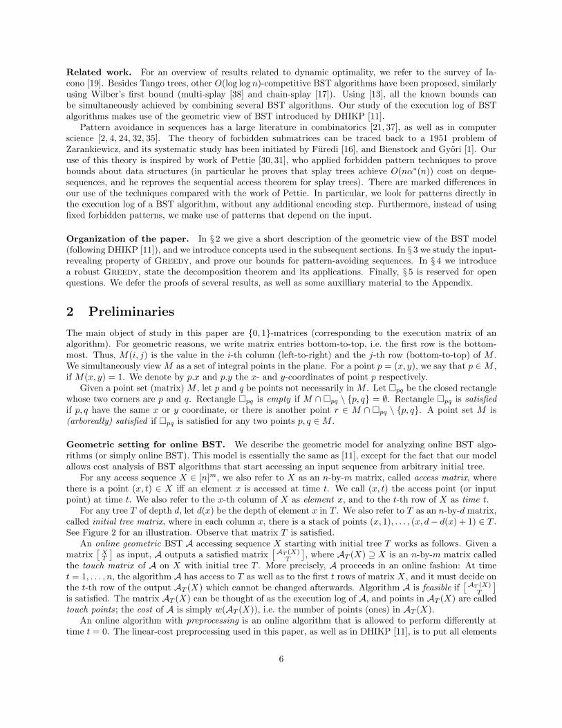
Consider the execution of an online BST A on sequence X with initial tree T just before time t. LetOt−1 denote the output at time t − 1 (i.e. the initial tree T and the first t − 1 rows of AT (X)). Letτ(b, t− 1) = max i | (b, i) ∈ Ot−1 for any b ∈ [n]. In words, τ(b, t− 1) is the last time strictly before t whenb is touched, otherwise it is a non-positive number defined by the initial tree. Let (a, t) ∈ X be the accesspoint at time t. We define stairt(a) as the set of elements b ∈ [n] for which (a,t),(b,τ(b,t−1)) is not satisfied.Greedy touches element x ∈ [n] if and only if x ∈ stairt(a). See Figure 2 for an illustration of stairs.

1 2 3 4 5 6 7 8 9 10 11 1 2 3 4 5 6 7 8 9 10 11

Figure 2: Tree-view and geometric view of initial tree. Search path and stair (at time 1) of element 5.

We define stairLeftt(a) = b ∈ stairt(a) | b < a and stairRightt(a) = b ∈ stairt(a) | b > a. Thealgorithms GreedyLeft and GreedyRight are analogous to Greedy, but they only touch stairLeftt(a),respectively stairRightt(a) for every time t; SGreedy simply refers to the union of the GreedyLeft andGreedyRight outputs, which is not necessarily satisfied. It is known [11, 18] that SGreedy constant-approximates the independent rectangle bound which subsumes the two previously known lower bounds onOPT, called Wilber’s first and second bounds [39].

Theorem 2.2 ( [11, 18, 39]). For any BST A (online or offline) that runs on sequence X with arbitraryinitial tree T , w(AT (X)) = Ω(SGreedy(X)).

A nice property of Greedy and SGreedy is that an element x can become “hidden” in some rangein the sense that if we do not access in x’s hidden range, then x will not be touched. Next, we formallydefine this concept, and list some cases when elements become hidden during the execution of Greedy andSGreedy. The concept is illustrated in Figure 4.

Definition 2.3 (Hidden). For any algorithm A, an element x is hidden in range [w, y] after t if, given thatthere is no access point p ∈ [w, y]× (t, t′] for any t′ > t, then x will not be touched by A in time (t, t′].

9with some minor additional argument about initial trees from Appendix C.1.10The statement holds unconditionally for offline algorithms, and under a mild assumption if we require Ap and A to be

online.

7

Figure 3: After time t, element x is hidden in (w, n] for Greedy, and in (w, x] for GreedyRight. After time t′,element x is hidden in (w, y) for Greedy; it is easy to verify that any access outside of [w, y] will nevertouch x.

Lemma 2.4 (Proof in Appendix B.1). Let x be some element.(i) If there is an element w < x where τ(w, t) ≥ τ(x, t), then x is hidden in (w, n] and (w, x] after t for

Greedy and GreedyRight respectively.(ii) If there is an element y > x where τ(y, t) ≥ τ(x, t), then x is hidden in [1, y) and [x, y) after t for

Greedy and GreedyLeft respectively.(iii) If there are elements w, y where w < x < y, and τ(w, t), τ(y, t) ≥ τ(x, t), then x is hidden in (w, y)

after t for Greedy.

Forbidden submatrix theory. Let M be an n-by-m matrix. Given I ⊆ [n] and J ⊆ [m], a submatrixM |I,J is obtained by removing columns in [n] \ I and rows in [m] \ J from M .

Definition 2.5 (Forbidden submatrix). Given a matrix M and another matrix P of size c× d, we say thatM contains P if there is a c × d submatrix M ′ of M such that M ′(i, j) = 1 whenever P (i, j) = 1. We saythat M avoids (forbids) P if M does not contain P .

We often call an avoided (forbidden) matrix a “pattern”. For any permutation π = (π1, . . . , πk) ∈ Sk,we also refer to π as a k-by-k matrix where (πi, i) ∈ π for all 1 ≤ i ≤ k. Permutation matrices have a singleone-entry in every row and in every column. Relaxing this condition slightly, we call a matrix that has asingle one in every column a light matrix. We make use of the following results.

Lemma 2.6. Let M and P be n-by-n and k-by-k matrices such that M avoids P .(i) (Marcus, Tardos [27], Fox [14]) If P is a permutation, the number of ones in M is at most n2O(k).

(ii) (Nivasch [?], Pettie [?]) If P is light, the number of ones in M is at most n2α(n)O(k)

.

We define the tensor product between matrices as follows: M ⊗ G is the matrix obtained by replacingeach one-entry of M by a copy of G, and replacing each zero-entry of M by an all-zero matrix equal in sizewith G. Suppose that M contains P . A bounding box B of P is a minimal submatrix M |I,J such that P iscontained in B, and I and J are sets of consecutive columns, resp. rows. We denote min(I), max(I), min(J),max(J), as B.xmin, B.xmax , B.ymin, B.ymax , respectively.

3 Greedy is input-revealing

In this section, we prove Theorems 1.1, 1.4, 1.6 and 1.7. We refer to § 1.1 for definitions of pattern-avoiding,k-decomposable and k-increasing permutations.

To bound the cost of algorithm A, we show that AT (X) (or A(X) if preprocessing is allowed) avoidssome pattern. In the following, Inck, Deck, and Altk are permutation matrices of size k, and Cap is a lightmatrix. These matrices will be defined later.

Lemma 3.1. Let X be an access sequence.

8

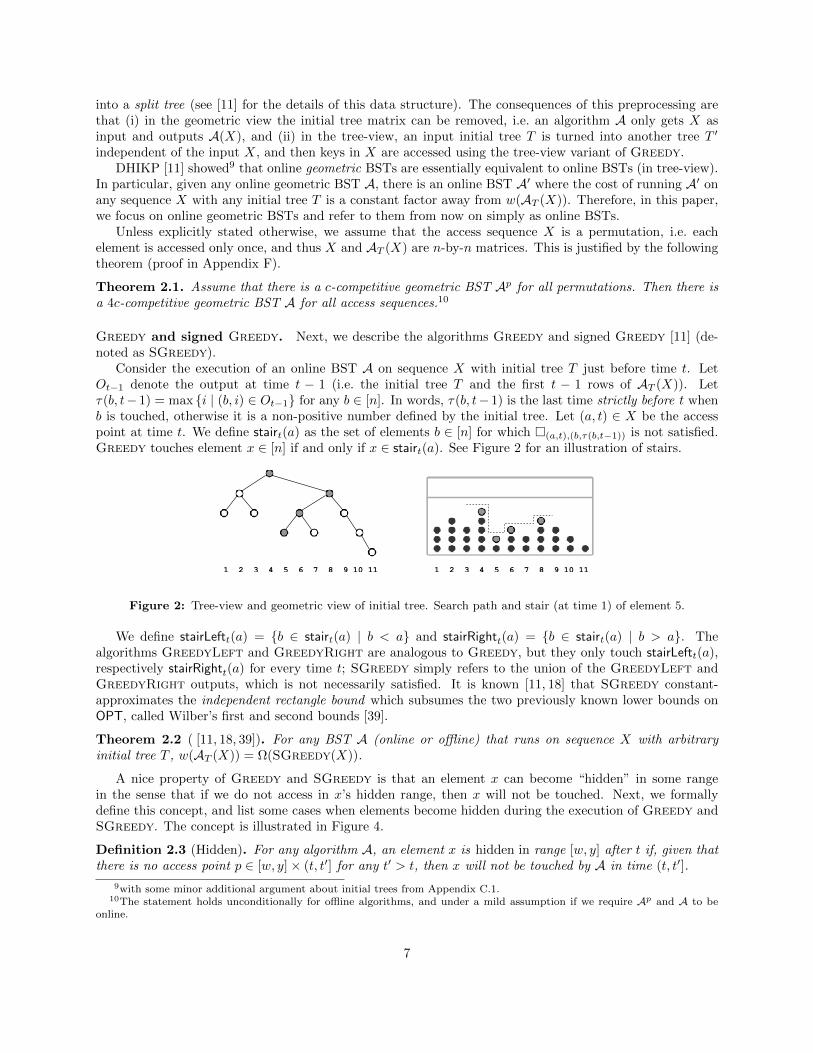
(i) If X avoids a permutation P of size k, then for any initial tree T , GreedyRightT (X), GreedyLeftT (X)and GreedyT (X) avoid P ⊗ (1, 2), P ⊗ (2, 1) and P ⊗ Cap respectively.

(ii) If X is k-increasing (k-decreasing), then for any initial tree T , GreedyT (X) avoids (k, . . . , 1)⊗Deck+1

((1, . . . , k)⊗ Inck+1).(iii) If X is k-decomposable, then Greedy(X) avoids P ⊗ Altk+4 for all simple permutations P of size at

least k + 1.

The application of Lemma 2.6 is sufficient to complete all the proofs, together with the observation that,for any permutation matrix P of size k × k, if G is a permutation (resp. light) matrix of size ` × `, thenP ⊗G is a permutation (resp. light) matrix of size k`× k`.

The rest of this section is devoted to the proof of Lemma 3.1. We need the definition of the input-revealinggadget which is a pattern whose existence in the touch matrix (where access points are indistinguishablefrom touch points) gives some information about the locations of access points.

Definition 3.2 (Input-revealing gadgets). Let X be an access matrix, A be an algorithm and A(X) be thetouch matrix of A running on X.– Capture Gadget. A pattern P is a capture gadget for algorithm A if, for any bounding box B of P inA(X), there is an access point p ∈ B.

– Monotone Gadget. A pattern P is a k-increasing (k-decreasing) gadget for algorithm A if, for anybounding box B of P in A(X), either (i) there is an access point p ∈ B or, (ii) there are k accesspoints p1, . . . , pk such that B.ymin ≤ p1.y < · · · < pk.y ≤ B.ymax and p1.x < · · · < pk.x < B.xmin(p1.x > · · · > pk.x > B.xmax ). In words, p1, . . . , pk form the pattern (1, . . . , k) (resp. (k, . . . , 1)).

– Alternating Gadget. A pattern P is a k-alternating gadget for algorithm A if, for any bounding box Bof P in A(X), either (i) there is an access point p ∈ B or, (ii) there are k access points p1, . . . , pk suchthat B.ymin ≤ p1.y < · · · < pk.y ≤ B.ymax and B.xmax < pi.x for all odd i and pi.x < B.xmin for alleven i.

Notice that if we had a permutation capture gadget G for algorithm A, we would be done: If X avoidspattern Q, then AT (X) avoids Q⊗G and forbidden submatrix theory applies. With arbitrary initial tree T , itis impossible to construct a permutation capture gadget for Greedy even for 2-decomposable sequences (seeAppendix H.1). Instead, we define a light capture gadget for Greedy for any sequence X and any initial treeT . Additionally, we construct permutation monotone and alternating gadgets. After a preprocessing step,we can use the alternating gadget to construct a permutation capture gadget for k-decomposable sequences.

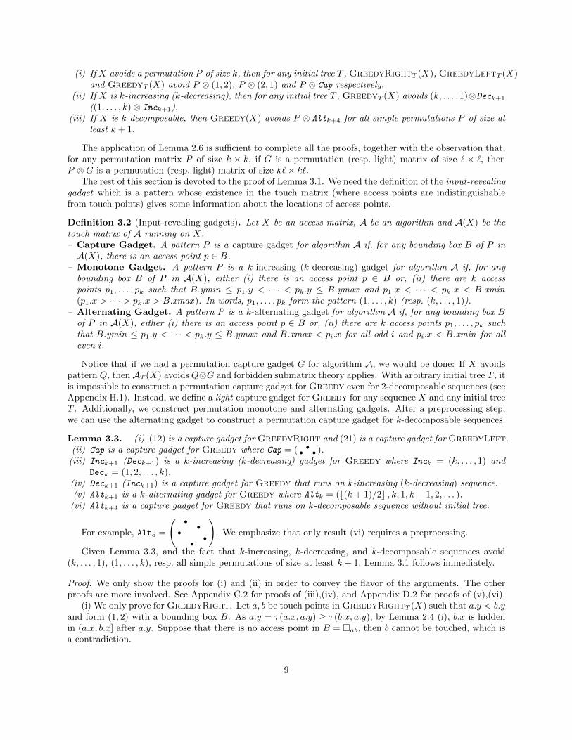
Lemma 3.3. (i) (12) is a capture gadget for GreedyRight and (21) is a capture gadget for GreedyLeft.(ii) Cap is a capture gadget for Greedy where Cap = ( •

• • ).(iii) Inck+1 (Deck+1) is a k-increasing (k-decreasing) gadget for Greedy where Inck = (k, . . . , 1) and

Deck = (1, 2, . . . , k).(iv) Deck+1 (Inck+1) is a capture gadget for Greedy that runs on k-increasing (k-decreasing) sequence.(v) Altk+1 is a k-alternating gadget for Greedy where Altk = (b(k + 1)/2c , k, 1, k − 1, 2, . . . ).

(vi) Altk+4 is a capture gadget for Greedy that runs on k-decomposable sequence without initial tree.

For example, Alt5 =

( ••

••

•

). We emphasize that only result (vi) requires a preprocessing.

Given Lemma 3.3, and the fact that k-increasing, k-decreasing, and k-decomposable sequences avoid(k, . . . , 1), (1, . . . , k), resp. all simple permutations of size at least k + 1, Lemma 3.1 follows immediately.

Proof. We only show the proofs for (i) and (ii) in order to convey the flavor of the arguments. The otherproofs are more involved. See Appendix C.2 for proofs of (iii),(iv), and Appendix D.2 for proofs of (v),(vi).

(i) We only prove for GreedyRight. Let a, b be touch points in GreedyRightT (X) such that a.y < b.yand form (1, 2) with a bounding box B. As a.y = τ(a.x, a.y) ≥ τ(b.x, a.y), by Lemma 2.4 (i), b.x is hiddenin (a.x, b.x] after a.y. Suppose that there is no access point in B = ab, then b cannot be touched, which isa contradiction.

9

(ii) Let a, b, c be touch points in GreedyT (X) such that a.x < b.x < c.x and a, b, c form Cap withbounding box B. As τ(a.x, a.y), τ(c.x, a.y) ≥ τ(b.x, a.y), by Lemma 2.4 (iii), b.x is hidden in (a.x, c.x) aftera.y. Suppose that there is no access point in B, then b cannot be touched, which is a contradiction.

4 Decomposition theorem and applications

In this section, we take a deeper look at decomposable permutations and investigate whether Greedy is“decomposable”, in the sense that one can bound the cost of Greedy on input sequences by summing overlocal costs on blocks. Proving such a property for Greedy seems to be prohibitively difficult (we illustratethis in Appendix H.1). Therefore, we propose a more “robust” but offline variant of Greedy which turnsout to be decomposable. We briefly describe the new algorithm, and state the main theorems and threeapplications, leaving the details to Appendix E.

Recursive decomposition. We refer the reader to § 1.1 for the definitions of blocks and recursive de-composition. Let S be a k-decomposable permutation access sequence, and let T be its (not necessarilyunique) decomposition tree (of arity at most k). Let P be a block in the decomposition tree T of S.Consider the subblocks P1, P2, . . . , Pk of P , and let P denote the unique permutation of size [k] that isorder-isomorphic to a sequence of arbitrary representative elements from the blocks P1, P2, . . . , Pk. We de-note P = P [P1, P2, . . . , Pk] a deflation of P , and we call P the skeleton of P . Visually, P is obtained fromP by contracting each block Pi to a single point. We associate with each block P (i.e. each node in T ) boththe corresponding rectangular region (in fact, a square), and the corresponding skeleton P (Figure 1). Wedenote the set of leaves and non-leaves of the tree T by L(T ) and N(T ) respectively.

Consider the k subblocks P1, . . . , Pk of a block P in this decomposition, numbered by increasing y-coordinate. We partition the rectangular region of P into k2 rectangular regions, whose boundaries arealigned with those of P1, . . . , Pk. We index these regions as R(i, j) with i going left to right and j goingbottom to top. In particular, the region R(i, j) is aligned (same y-coordinates) with Pj .

A robust version of Greedy. The main difficulty in analyzing the cost of Greedy on decomposable ac-cess sequences is the “interference” between different blocks of the decomposition. Our RGreedy algorithmis an extension of Greedy. Locally it touches at least those points that Greedy would touch; additionallyit may touch other points, depending on the recursive decomposition of the access sequence (this a prioriknowledge of the decomposition tree is what makes RGreedy an offline algorithm). The purpose of touchingextra points is to “seal off” the blocks, limiting their effect to the outside.

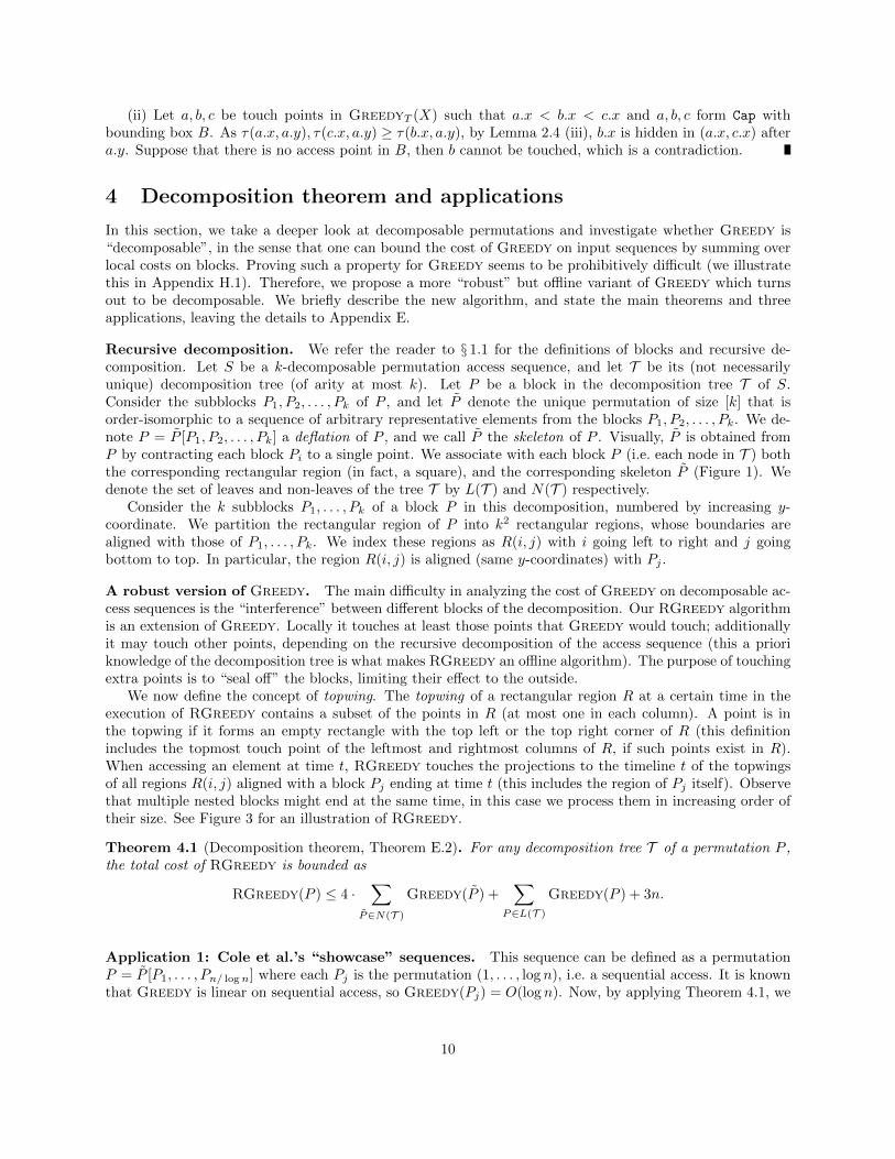
We now define the concept of topwing. The topwing of a rectangular region R at a certain time in theexecution of RGreedy contains a subset of the points in R (at most one in each column). A point is inthe topwing if it forms an empty rectangle with the top left or the top right corner of R (this definitionincludes the topmost touch point of the leftmost and rightmost columns of R, if such points exist in R).When accessing an element at time t, RGreedy touches the projections to the timeline t of the topwingsof all regions R(i, j) aligned with a block Pj ending at time t (this includes the region of Pj itself). Observethat multiple nested blocks might end at the same time, in this case we process them in increasing order oftheir size. See Figure 3 for an illustration of RGreedy.

Theorem 4.1 (Decomposition theorem, Theorem E.2). For any decomposition tree T of a permutation P ,the total cost of RGreedy is bounded as

RGreedy(P ) ≤ 4 ·∑

P∈N(T )

Greedy(P ) +∑

P∈L(T )

Greedy(P ) + 3n.

Application 1: Cole et al.’s “showcase” sequences. This sequence can be defined as a permutationP = P [P1, . . . , Pn/ logn] where each Pj is the permutation (1, . . . , log n), i.e. a sequential access. It is knownthat Greedy is linear on sequential access, so Greedy(Pj) = O(log n). Now, by applying Theorem 4.1, we

10

Figure 4: Illustration of RGreedy. Left: region with points and topwing highlighted. Right: a sample run ofRGreedy on a 2-decomposable input. Access points are dark circles, points touched by Greedy are graycircles, points touched by the RGreedy augmentation are gray squares. The access point in the topmostline completes the black square and also the enclosing gray square. The topwing of the black squareconsists of the black circle at position (1,6) and the gray circle at (3,5). Therefore the augmentation ofthe black square adds the gray square at (3,6). The topwing of R(2, 2) consists of the gray circle at (4,4)and hence the gray square at (4,6) is added. The topwing of the gray square consists of points (1,6) and(6,3); the point (4,4) does not belong to the topwing because (4,6) has already been added. Therefore,the gray square at (6,6) is added.

can say that the cost of RGreedy on P is RGreedy(P ) ≤ 4 · Greedy(P ) +∑j Greedy(Pj) + O(n) ≤

O( nlogn · log( n

logn )) + nlognO(log n) +O(n) = O(n). This implies the linear optima of this class of sequences.

Application 2: Simple permutations as the “core” difficulty of BST inputs. We prove that, ifGreedy is c-competitive on simple permutations, then RGreedy is O(c)-approximate for all permutations.To prove this, we consider a block decomposition tree T in which the permutation corresponding to everynode is simple. Using Theorem 4.1 and the hypothesis that Greedy is c-competitive for simple permutations:

RGreedy(P ) ≤ 4c ·∑

P∈N(T )

OPT(P ) + c ·∑

P∈L(T )

OPT(P ) + 3n.

Now we decompose OPT into subproblems the same way as done for RGreedy. We prove in Lemma E.4that OPT(P ) ≥

∑P∈T OPT(P )−2n. Combined with Theorem 4.1 this yields RGreedy(P ) ≤ 4c·OPT(P )+

(8c+ 3)n. Using Theorem 2.1 we can extend this statement to arbitrary access sequences.

Application 3: Recursively decomposable permutations. Let X be a k-decomposable permutation.Then there is a decomposition tree T of X in which each node is a permutation of size at most k. Each blockP ∈ L(T ) ∪ N(T ) has Greedy(P ) = O(|P | log |P |) = O(|P | log k). By standard charging arguments, thesum

∑P∈N(T )∪L(T ) |P | = O(n), so the total cost of RGreedy is O(n log k); see the full proof in Appendix E.

We remark that the logarithmic dependence on k is optimal (Proof in Appendix H.2), and that Greedyasymptotically matches this bound when k is constant (Theorem 1.4).

11

5 Discussion and open questions

Besides the long-standing open question of resolving dynamic optimality, our work raises several new onesin the context of pattern avoidance. We list some that are most interesting to us.

Can the bound of Theorem 1.1 be improved? While our input-revealing techniques are unlikely to yielda linear bound (Appendix H.1), a slight improvement could come from strengthening Lemma 2.6(ii) for thespecial kind of light matrices that arise in our proof.

An intriguing question is whether there is a natural characterization of all sequences with linear optimum.How big is the overlap between “easy inputs” and inputs with pattern avoidance properties? We haveshown that avoidance of a small pattern makes sequences easy. The converse does not hold: There is apermutation X ∈ Sn with k(X) =

√n but for which Greedy(X) = O(n); see Appendix H.3. Note that

our pattern-avoiding properties are incomparable with the earlier parametrizations (e.g. dynamic finger); seeAppendix H.3. Is there a parameter that subsumes both pattern-avoidance and dynamic finger?

A question directly related to our work is to close the gap between OPT = O(n log k) and n2O(k2) byGreedy on k-decomposable sequences (when k = ω(1)). Matching the optimum (if at all possible) likelyrequires novel techniques: splay is not even known to be linear on preorder sequences with preprocessing,and with forbidden-submatrix-arguments it seems impossible to obtain bounds beyond11 O(nk).

We proved that if Greedy is optimal on simple permutations, then RGreedy is optimal on all accesssequences. Can some property of simple permutations12 be algorithmically exploited? Can RGreedy bemade online? Can our application for Cole’s showcase sequence be extended in order to prove the dynamicfinger property for Greedy?

Finally, making further progress on the traversal conjecture will likely require novel ideas. We proposea simpler question that captures the barrier for three famous conjectures: traversal, deque, and split (Ap-pendix H.4). Given any initial tree T , access a preorder sequence defined by a path P (a BST where eachnon-leaf node has a single child). Prove a linear bound for your favorite online BST!

11An n-by-n matrix avoiding all permutations of size at least k can contain Ω(nk) ones.12Note that simple permutations can have linear cost. In Appendix H.3 we show such an example.

12

References

[1] Daniel Bienstock and Ervin Gyori. An extremal problem on sparse 0-1 matrices. SIAM J. DiscreteMath., 4(1):17–27, 1991. 5

[2] Prosenjit Bose, Jonathan F Buss, and Anna Lubiw. Pattern matching for permutations. InformationProcessing Letters, 65(5):277–283, 1998. 3, 5

[3] Robert Brignall. A survey of simple permutations. CoRR, abs/0801.0963, 2008. 3, 20, 25

[4] Marie-Louise Bruner and Martin Lackner. The computational landscape of permutation patterns.CoRR, abs/1301.0340, 2013. 5

[5] Mihai Badoiu, Richard Cole, Erik D. Demaine, and John Iacono. A unified access bound on comparison-based dynamic dictionaries. Theoretical Computer Science, 382(2):86–96, August 2007. Special issue ofselected papers from the 6th Latin American Symposium on Theoretical Informatics, 2004. 32

[6] P. Chalermsook, M. Goswami, L. Kozma, K. Mehlhorn, and T. Saranurak. A global geometric view ofsplaying. To Appear, CoRR abs/1503.03105, 2015. 2

[7] P. Chalermsook, M. Goswami, L. Kozma, K. Mehlhorn, and T. Saranurak. Greedy is an almost optimaldeque. To Appear, 2015. 2

[8] R. Chaudhuri and H. Hoft. Splaying a search tree in preorder takes linear time. SIGACT News,24(2):88–93, April 1993. 1

[9] R. Cole. On the dynamic finger conjecture for splay trees. part ii: The proof. SIAM Journal onComputing, 30(1):44–85, 2000. 1, 2

[10] Richard Cole, Bud Mishra, Jeanette Schmidt, and Alan Siegel. On the dynamic finger conjecture forsplay trees. part i: Splay sorting log n-block sequences. SIAM J. Comput., 30(1):1–43, April 2000. 1,2, 4, 25

[11] Erik D. Demaine, Dion Harmon, John Iacono, Daniel M. Kane, and Mihai Patrascu. The geometry ofbinary search trees. In SODA 2009, pages 496–505, 2009. 1, 3, 4, 5, 6, 7, 18

[12] Erik D. Demaine, Dion Harmon, John Iacono, and Mihai Patrascu. Dynamic optimality - almost. SIAMJ. Comput., 37(1):240–251, 2007. 1

[13] Erik D. Demaine, John Iacono, Stefan Langerman, and Ozgur Ozkan. Combining binary search trees. InAutomata, Languages, and Programming - 40th International Colloquium, ICALP 2013, Riga, Latvia,July 8-12, 2013, Proceedings, Part I, pages 388–399, 2013. 5

[14] Jacob Fox. Stanley-Wilf limits are typically exponential. CoRR, pages –1–1, 2013. 7

[15] Kyle Fox. Upper bounds for maximally greedy binary search trees. In WADS 2011, pages 411–422,2011. 1, 2

[16] Zoltan Furedi. The maximum number of unit distances in a convex n-gon. J. Comb. Theory, Ser. A,55(2):316–320, 1990. 5

[17] George F. Georgakopoulos. Chain-splay trees, or, how to achieve and prove loglogn-competitiveness bysplaying. Inf. Process. Lett., 106(1):37–43, 2008. 5

[18] Dion Harmon. New Bounds on Optimal Binary Search Trees. PhD thesis, Massachusetts Institute ofTechnology, 2006. 7

13

[19] John Iacono. In pursuit of the dynamic optimality conjecture. In Andrej Brodnik, Alejandro Lopez-Ortiz, Venkatesh Raman, and Alfredo Viola, editors, Space-Efficient Data Structures, Streams, andAlgorithms, volume 8066 of Lecture Notes in Computer Science, pages 236–250. Springer Berlin Heidel-berg, 2013. 5

[20] Balazs Keszegh. On linear forbidden submatrices. Journal of Combinatorial Theory, Series A, 116(1):232– 241, 2009. 7

[21] S. Kitaev. Patterns in Permutations and Words. Monographs in Theoretical Computer Science. AnEATCS Series. Springer, 2011. 1, 5

[22] Martin Klazar. The Furedi-Hajnal conjecture implies the Stanley-Wilf conjecture. In Daniel Krob,AlexanderA. Mikhalev, and AlexanderV. Mikhalev, editors, Formal Power Series and Algebraic Com-binatorics, pages 250–255. Springer Berlin Heidelberg, 2000. 7

[23] D.E. Knuth. Optimum binary search trees. Acta Informatica, 1(1):14–25, 1971. 1

[24] Donald E. Knuth. The Art of Computer Programming, Volume I: Fundamental Algorithms. Addison-Wesley, 1968. 1, 5

[25] Joan M. Lucas. Canonical forms for competitive binary search tree algorithms. Tech. Rep. DCS-TR-250,Rutgers University, 1988. 1

[26] Joan M. Lucas. On the competitiveness of splay trees: Relations to the union-find problem. On-line Algorithms, DIMACS Series in Discrete Mathematics and Theoretical Computer Science, 7:95–124,1991. In Lyle A. McGeoch and Daniel D. Sleator, editors. 34

[27] Adam Marcus and Gabor Tardos. Excluded permutation matrices and the Stanley-Wilf conjecture.Journal of Combinatorial Theory, Series A, 107(1):153 – 160, 2004. 7

[28] Kurt Mehlhorn. Nearly optimal binary search trees. Acta Informatica, 5(4):287–295, 1975. 1

[29] J.Ian Munro. On the competitiveness of linear search. In Mike S. Paterson, editor, Algorithms - ESA2000, volume 1879 of Lecture Notes in Computer Science, pages 338–345. Springer Berlin Heidelberg,2000. 1

[30] Seth Pettie. Splay trees, Davenport-Schinzel sequences, and the deque conjecture. In Proceedings ofthe Nineteenth Annual ACM-SIAM Symposium on Discrete Algorithms, SODA ’08, pages 1115–1124,Philadelphia, PA, USA, 2008. Society for Industrial and Applied Mathematics. 1, 2, 5

[31] Seth Pettie. Applications of forbidden 0-1 matrices to search tree and path compression-based datastructures. In Moses Charikar, editor, Proceedings of the Twenty-First Annual ACM-SIAM Symposiumon Discrete Algorithms, SODA 2010, Austin, Texas, USA, January 17-19, 2010, pages 1457–1467.SIAM, 2010. 2, 5

[32] Vaughan R. Pratt. Computing permutations with double-ended queues, parallel stacks and parallelqueues. In Proceedings of the Fifth Annual ACM Symposium on Theory of Computing, STOC ’73,pages 268–277, New York, NY, USA, 1973. ACM. 5

[33] James H. Schmerl and William T. Trotter. Critically indecomposable partially ordered sets, graphs,tournaments and other binary relational structures. Discrete Mathematics, 113(13):191 – 205, 1993. 20

[34] Daniel Dominic Sleator and Robert Endre Tarjan. Self-adjusting binary search trees. J. ACM, 32(3):652–686, July 1985. 1, 2, 34

[35] Robert Endre Tarjan. Sorting using networks of queues and stacks. J. ACM, 19(2):341–346, April 1972.5

14

[36] Robert Endre Tarjan. Sequential access in splay trees takes linear time. Combinatorica, 5(4):367–378,1985. 1, 2, 34

[37] Vincent Vatter. Permutation classes. CoRR, abs/1409.5159, 2014. 1, 5

[38] Chengwen C. Wang, Jonathan C. Derryberry, and Daniel D. Sleator. O(log log n)-competitive dynamicbinary search trees. In Proceedings of the Seventeenth Annual ACM-SIAM Symposium on DiscreteAlgorithm, SODA ’06, pages 374–383, Philadelphia, PA, USA, 2006. Society for Industrial and AppliedMathematics. 2, 5

[39] R. Wilber. Lower bounds for accessing binary search trees with rotations. SIAM Journal on Computing,18(1):56–67, 1989. 4, 7

15

A Warmup: A direct proof for preorder sequences

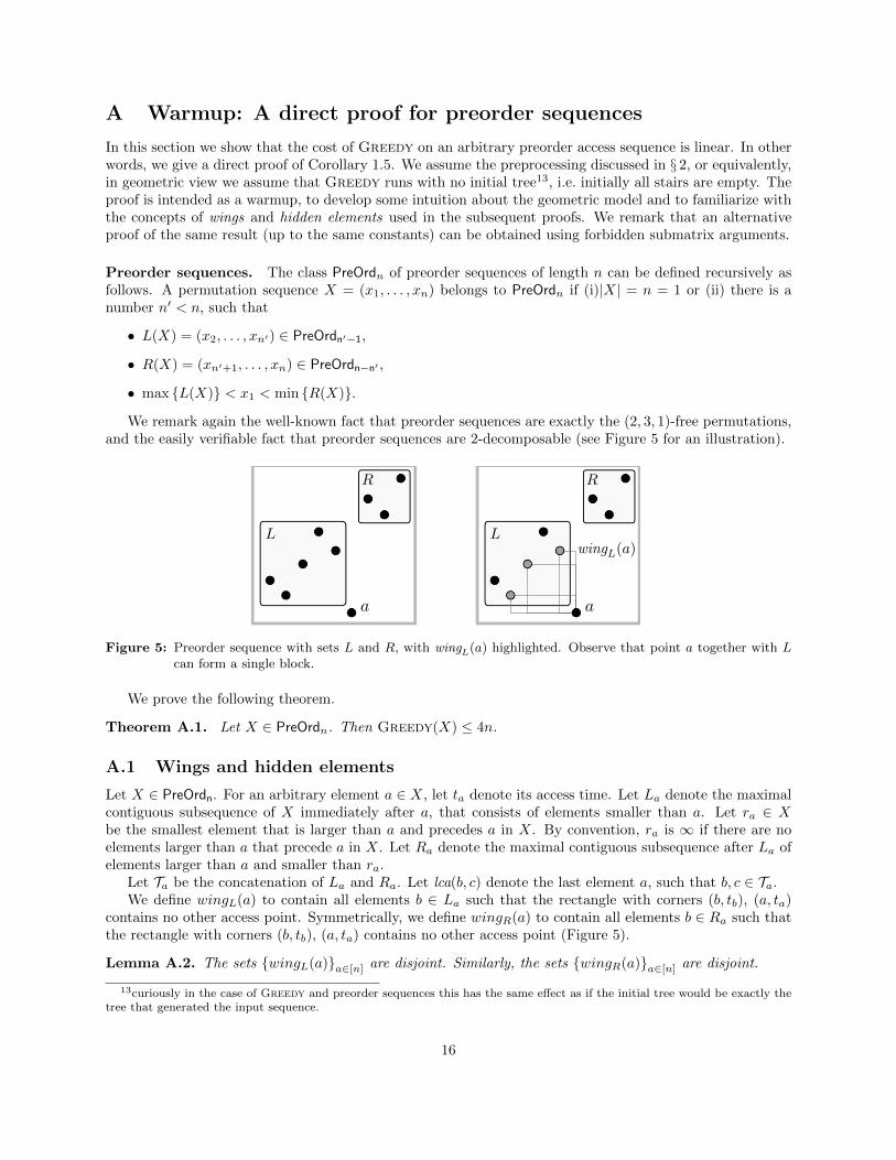
In this section we show that the cost of Greedy on an arbitrary preorder access sequence is linear. In otherwords, we give a direct proof of Corollary 1.5. We assume the preprocessing discussed in § 2, or equivalently,in geometric view we assume that Greedy runs with no initial tree13, i.e. initially all stairs are empty. Theproof is intended as a warmup, to develop some intuition about the geometric model and to familiarize withthe concepts of wings and hidden elements used in the subsequent proofs. We remark that an alternativeproof of the same result (up to the same constants) can be obtained using forbidden submatrix arguments.

Preorder sequences. The class PreOrdn of preorder sequences of length n can be defined recursively asfollows. A permutation sequence X = (x1, . . . , xn) belongs to PreOrdn if (i)|X| = n = 1 or (ii) there is anumber n′ < n, such that

• L(X) = (x2, . . . , xn′) ∈ PreOrdn′−1,

• R(X) = (xn′+1, . . . , xn) ∈ PreOrdn−n′ ,

• max L(X) < x1 < min R(X).

We remark again the well-known fact that preorder sequences are exactly the (2, 3, 1)-free permutations,and the easily verifiable fact that preorder sequences are 2-decomposable (see Figure 5 for an illustration).

Figure 5: Preorder sequence with sets L and R, with wingL(a) highlighted. Observe that point a together with Lcan form a single block.

We prove the following theorem.

Theorem A.1. Let X ∈ PreOrdn. Then Greedy(X) ≤ 4n.

A.1 Wings and hidden elements

Let X ∈ PreOrdn. For an arbitrary element a ∈ X, let ta denote its access time. Let La denote the maximalcontiguous subsequence of X immediately after a, that consists of elements smaller than a. Let ra ∈ Xbe the smallest element that is larger than a and precedes a in X. By convention, ra is ∞ if there are noelements larger than a that precede a in X. Let Ra denote the maximal contiguous subsequence after La ofelements larger than a and smaller than ra.

Let Ta be the concatenation of La and Ra. Let lca(b, c) denote the last element a, such that b, c ∈ Ta.We define wingL(a) to contain all elements b ∈ La such that the rectangle with corners (b, tb), (a, ta)

contains no other access point. Symmetrically, we define wingR(a) to contain all elements b ∈ Ra such thatthe rectangle with corners (b, tb), (a, ta) contains no other access point (Figure 5).

Lemma A.2. The sets wingL(a)a∈[n] are disjoint. Similarly, the sets wingR(a)a∈[n] are disjoint.

13curiously in the case of Greedy and preorder sequences this has the same effect as if the initial tree would be exactly thetree that generated the input sequence.

16

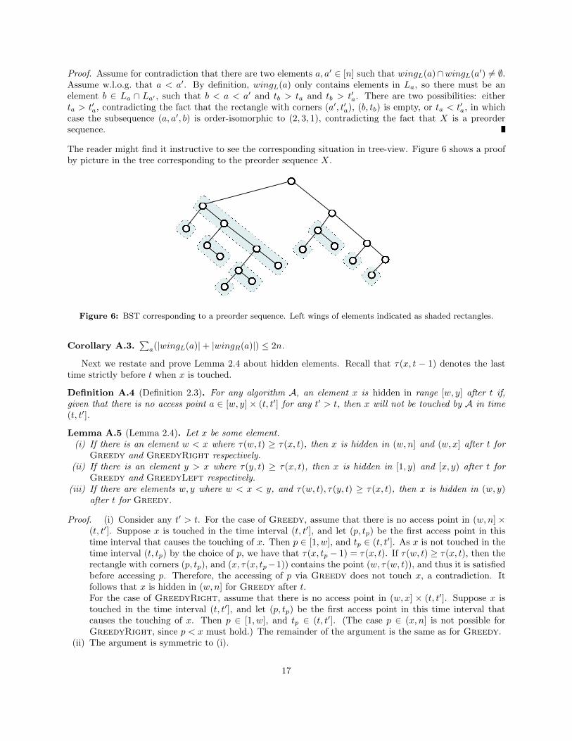
Proof. Assume for contradiction that there are two elements a, a′ ∈ [n] such that wingL(a)∩wingL(a′) 6= ∅.Assume w.l.o.g. that a < a′. By definition, wingL(a) only contains elements in La, so there must be anelement b ∈ La ∩ La′ , such that b < a < a′ and tb > ta and tb > t′a. There are two possibilities: eitherta > t′a, contradicting the fact that the rectangle with corners (a′, t′a), (b, tb) is empty, or ta < t′a, in whichcase the subsequence (a, a′, b) is order-isomorphic to (2, 3, 1), contradicting the fact that X is a preordersequence.

The reader might find it instructive to see the corresponding situation in tree-view. Figure 6 shows a proofby picture in the tree corresponding to the preorder sequence X.

Figure 6: BST corresponding to a preorder sequence. Left wings of elements indicated as shaded rectangles.

Corollary A.3.∑a(|wingL(a)|+ |wingR(a)|) ≤ 2n.

Next we restate and prove Lemma 2.4 about hidden elements. Recall that τ(x, t − 1) denotes the lasttime strictly before t when x is touched.

Definition A.4 (Definition 2.3). For any algorithm A, an element x is hidden in range [w, y] after t if,given that there is no access point a ∈ [w, y]× (t, t′] for any t′ > t, then x will not be touched by A in time(t, t′].

Lemma A.5 (Lemma 2.4). Let x be some element.(i) If there is an element w < x where τ(w, t) ≥ τ(x, t), then x is hidden in (w, n] and (w, x] after t for

Greedy and GreedyRight respectively.(ii) If there is an element y > x where τ(y, t) ≥ τ(x, t), then x is hidden in [1, y) and [x, y) after t for

Greedy and GreedyLeft respectively.(iii) If there are elements w, y where w < x < y, and τ(w, t), τ(y, t) ≥ τ(x, t), then x is hidden in (w, y)

after t for Greedy.

Proof. (i) Consider any t′ > t. For the case of Greedy, assume that there is no access point in (w, n] ×(t, t′]. Suppose x is touched in the time interval (t, t′], and let (p, tp) be the first access point in thistime interval that causes the touching of x. Then p ∈ [1, w], and tp ∈ (t, t′]. As x is not touched in thetime interval (t, tp) by the choice of p, we have that τ(x, tp − 1) = τ(x, t). If τ(w, t) ≥ τ(x, t), then therectangle with corners (p, tp), and (x, τ(x, tp−1)) contains the point (w, τ(w, t)), and thus it is satisfiedbefore accessing p. Therefore, the accessing of p via Greedy does not touch x, a contradiction. Itfollows that x is hidden in (w, n] for Greedy after t.For the case of GreedyRight, assume that there is no access point in (w, x] × (t, t′]. Suppose x istouched in the time interval (t, t′], and let (p, tp) be the first access point in this time interval thatcauses the touching of x. Then p ∈ [1, w], and tp ∈ (t, t′]. (The case p ∈ (x, n] is not possible forGreedyRight, since p < x must hold.) The remainder of the argument is the same as for Greedy.

(ii) The argument is symmetric to (i).

17

(iii) Consider any t′ > t. Assume that there is no access point in (w, y)× (t, t′]. Suppose x is touched in thetime interval (t, t′], and let (p, tp) be the first access point in this time interval that causes the touchingof x. There are two cases. If p ∈ [1, w], we use the argument of (i). If p ∈ [y, n], we use the argumentof (ii).

A.2 Bounding the cost of Greedy

Lemma A.6. For any element c ∈ La\wingL(a), a is not touched when accessing c using Greedy. Similarlyfor c ∈ Ra \ wingR(a).

Proof. There must be an access point b, such that c < b < a and ta < tb < tc, for otherwise c would be inwingL(a). Since τ(b, tb) ≥ τ(a, tb), it follows that a is hidden in (b, n] after tb. All accesses in the interval(tb, tc] are in [c, b). Hence, a is not touched.

Corollary A.7. Let a be any element. Greedy touches a when accessing elements in Ta at most |wingL(a)|+|wingR(a)| times.

Lemma A.8. Let a be any element. Greedy touches a when accessing elements outside Ta at most once.

Proof. No element is touched before it is accessed. Since the elements in Ta are accessed consecutively, weonly need to consider accesses after all elements in Ta have been accessed. All such accesses are to elementsto the right of Ta. Let c be the first element accessed after the last access to an element in Ta and letb = lca(a, c). Then a ∈ Lb, and c is the first element in Rb.

Since Tc contains all elements in (b, c], Greedy does not touch any element in (b, c] before time tc. Letd be the element in (a, b] with largest time τ(d, tc − 1). If there are several such d, let d be the rightmostsuch element. Since no element in (b, c] is accessed before time tc, d is also the rightmost element in (a, c]with largest time τ(d, tc − 1). The rectangle with corners (d, τ(d, tc − 1)) and (c, tc) contains no other pointand hence d is touched at time tc.

Clearly, τ(a, tc) ≤ tc = τ(d, tc). Thus a is hidden in [1, d) after time tc and hence a is not touched aftertime tc.

Corollary B.7 and Lemma B.8 together imply that each element a is only touched at most |wingL(a)|+|wingR(a)|+ 1 times, so the total cost is at most

∑a∈[n](|wingL(a)|+ |wingR(a)|+ 2) ≤ 4n. This concludes

the proof of Theorem B.1.

B Access sequences with initial trees

B.1 Initial trees.

In the BST model, the initial tree is the state of the BST before the first element is accessed. In the tree-viewof BST execution, we know the structure of the tree exactly in every time step, and hence the structureof the initial tree as well. This is less obvious, however, in the geometric view. In fact, according to thereduction of DHIKP, the initial tree is always a split tree [11], hidden from us in geometric view. We showhow to “force” an arbitrary initial tree into the geometric view of BST execution.

First, we observe a simple fact. Given a binary search tree T , we denote the search path of an element ain T as path(a, T ). It is easy to show that two BSTs T1 and T2, containing [n], have the same structure iffpath(a, T1) = path(a, T2) as a set, for all a ∈ [n].

The stair of an element is, in some sense, the geometric view of the search path. Indeed, path(a, T ) = b | bis touched if a is accessed in T. Similarly, stairt(a) = b | b is touched if a is accessed at time t. Thus, tomodel an initial tree T into the geometric view, it is enough to enforce that stair1(a) = path(a, T ).

We can achieve this in a straightforward way, by putting stacks of points in each column below the firstrow, corresponding to the structure of the initial tree T . More precisely, in column x we put a stack of height

18

d− d(x) + 1, where d(x) is the depth of element x in T , and d is the maximum depth of an element (Figure2). One can easily show that stair1(a) = path(a,T) for all a ∈ [n].

We remark that the points representing the initial tree are not counted in the cost.

B.2 k-increasing sequences

We prove Lemma 3.3 (iii) and (iv).

Lemma B.1 (Lemma 3.3(iii)). Inck+1 (Deck+1) is a k-increasing (k-decreasing) gadget for Greedy whereInck = (k, . . . , 1) and Deck = (1, 2, . . . , k).

Proof. We only prove that Inck+1 is a k-increasing gadget. Let q0, . . . , qk be touch points in GreedyT (X)such that qi.y < qi+1.y for all i and form Inck+1 with bounding box B. Note that, for all 1 ≤ i ≤ k, we canassume that there is no touch point q′i where q′i.x = qi.x and qi−1.y < q′i.y < qi.y, otherwise we can chooseq′i instead of qi. So, for any t ∈ [qi−1.y, qi.y) we have that τ(qi−1.x, t) ≥ τ(qi.x, t) for all 1 ≤ i ≤ k. Supposethat there is no access point in B.

By Lemma 2.4 (ii), q1.x is hidden in [1, q0.x) after q0.y. So there must be an access point p1 ∈ [1, B.xmin)×(q0.y, q1.y], otherwise q1 cannot be touched. We choose such p1 where p1.x is maximized. If p1.y < q1.y,then τ(p1.x, p1.y), τ(q0.x, p1.y) ≥ τ(q1.x, p1.y). So by Lemma 2.4 (iii), q1.x is hidden in (p1.x, q0.x) after p1.yand hence q1 cannot be touched, which is a contradiction. So we have p1.y = q1.y and p1.x < B.xmin.

Next, we prove by induction from i = 2 to k that, given the access point pi−1 where pi−1.y = qi−1.y andpi−1.x < B.xmin, there must be an access point pi where pi.y = qi.y and pi−1.x < pi.x < B.xmin. Again,by Lemma 2.4 (iii), there must be an access point pi ∈ (pi−1.x, qi−1.x)× (qi−1.y, qi.y] otherwise qi cannot betouched. We choose the point pi where pi.x is maximized. If pi.y < qi.y, then τ(pi.x, pi.y), τ(qi−1.x, pi.y) ≥τ(qi.x, pi.y). So by Lemma 2.4 (iii), qi.x is hidden in (pi.x, qi−1.x) after pi.y and hence qi cannot be touched.So we have pi.y = qi.y and pi−1.x < pi.x < B.xmin. Therefore, we get p1.x < · · · < pk.x < B.xmin whichconcludes the proof.

Lemma B.2 (Lemma 3.3(iv)). Deck+1 (Inck+1) is a capture gadget for Greedy that runs on k-increasing(k-decreasing) sequence.

Proof. We only prove that Inck+1 is a capture gadget for Greedy running on k-decreasing sequence X.Since Inck+1 is an increasing gadget, if Inck+1 appears in GreedyT (X) with bounding box B, then eitherthere is an access point in B or there are access points forming (1, 2, . . . , k). The latter case cannot happenbecause X avoids (1, 2, . . . , k). So Inck+1 is a capture gadget.

C Access sequences without initial trees: k-decomposable permu-tations

C.1 Pattern avoidance and recursive decomposability

We restate and prove Lemma 1.3 that connects the k-decomposability of a permutation with pattern avoid-ance properties.

Lemma C.1 (Extended form of Lemma 1.3). Let P be a permutation, and let k be an integer. The followingstatements are equivalent:

(i) P is k-decomposable,

(ii) P avoids all simple permutations of size at least k + 1,

(iii) P avoids all simple permutations of size k + 1 and k + 2.

19

Proof. (ii) =⇒ (iii) is obvious.(iii) =⇒ (ii) follows from the result of Schmerl and Trotter [33] that every simple permutation of length

n contains a simple permutation of length n − 1 or n − 2, and the simple observation that if P avoids Q,then P also avoids all permutations containing Q.

(ii) =⇒ (i) follows from the observation that a permutation P contains all permutations in its blockdecomposition tree TP . Further, it is known [3] that every permutation P has a block decomposition treeTP in which all nodes are simple permutations. If P contains no simple permutation of size k + 1 or more,it must have a block decomposition tree in which all nodes are simple permutations of size at most k, it istherefore, k-decomposable.

(i) =⇒ (ii): we show the contrapositive ¬(ii) =⇒ ¬(i). Indeed, if P contains a simple permutationQ of size at least k + 1, then any k-decomposition of P would induce a k-decomposition of Q, contradictingthe fact that Q is simple.

C.2 k-decomposable permutations

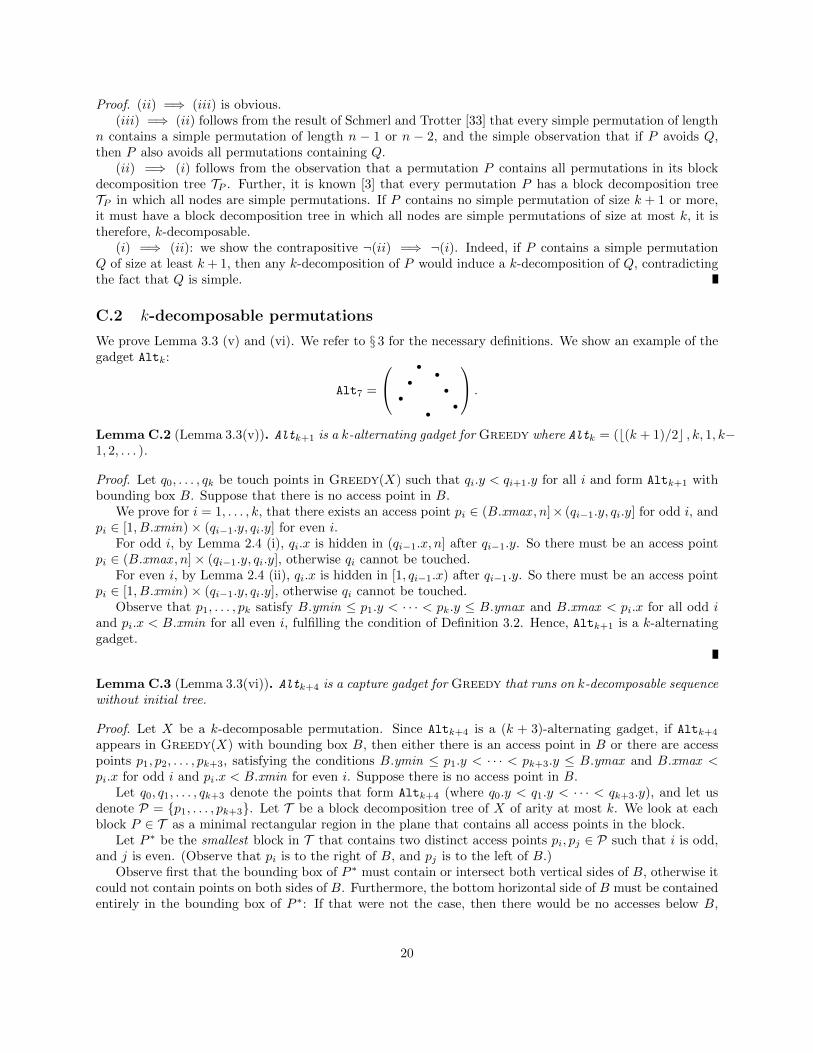
We prove Lemma 3.3 (v) and (vi). We refer to § 3 for the necessary definitions. We show an example of thegadget Altk:

Alt7 =

••

••

••

•

.

Lemma C.2 (Lemma 3.3(v)). Altk+1 is a k-alternating gadget for Greedy where Altk = (b(k + 1)/2c , k, 1, k−1, 2, . . . ).

Proof. Let q0, . . . , qk be touch points in Greedy(X) such that qi.y < qi+1.y for all i and form Altk+1 withbounding box B. Suppose that there is no access point in B.

We prove for i = 1, . . . , k, that there exists an access point pi ∈ (B.xmax , n]× (qi−1.y, qi.y] for odd i, andpi ∈ [1, B.xmin)× (qi−1.y, qi.y] for even i.

For odd i, by Lemma 2.4 (i), qi.x is hidden in (qi−1.x, n] after qi−1.y. So there must be an access pointpi ∈ (B.xmax , n]× (qi−1.y, qi.y], otherwise qi cannot be touched.

For even i, by Lemma 2.4 (ii), qi.x is hidden in [1, qi−1.x) after qi−1.y. So there must be an access pointpi ∈ [1, B.xmin)× (qi−1.y, qi.y], otherwise qi cannot be touched.

Observe that p1, . . . , pk satisfy B.ymin ≤ p1.y < · · · < pk.y ≤ B.ymax and B.xmax < pi.x for all odd iand pi.x < B.xmin for all even i, fulfilling the condition of Definition 3.2. Hence, Altk+1 is a k-alternatinggadget.

Lemma C.3 (Lemma 3.3(vi)). Altk+4 is a capture gadget for Greedy that runs on k-decomposable sequencewithout initial tree.

Proof. Let X be a k-decomposable permutation. Since Altk+4 is a (k + 3)-alternating gadget, if Altk+4

appears in Greedy(X) with bounding box B, then either there is an access point in B or there are accesspoints p1, p2, . . . , pk+3, satisfying the conditions B.ymin ≤ p1.y < · · · < pk+3.y ≤ B.ymax and B.xmax <pi.x for odd i and pi.x < B.xmin for even i. Suppose there is no access point in B.

Let q0, q1, . . . , qk+3 denote the points that form Altk+4 (where q0.y < q1.y < · · · < qk+3.y), and let usdenote P = p1, . . . , pk+3. Let T be a block decomposition tree of X of arity at most k. We look at eachblock P ∈ T as a minimal rectangular region in the plane that contains all access points in the block.

Let P ∗ be the smallest block in T that contains two distinct access points pi, pj ∈ P such that i is odd,and j is even. (Observe that pi is to the right of B, and pj is to the left of B.)

Observe first that the bounding box of P ∗ must contain or intersect both vertical sides of B, otherwise itcould not contain points on both sides of B. Furthermore, the bottom horizontal side of B must be containedentirely in the bounding box of P ∗: If that were not the case, then there would be no accesses below B,

20

and q0 (the lowest point of Altk+4) would not be touched by Greedy (since there is no initial tree). Thefollowing is the key observation of the proof.

Lemma C.4. Let k′ be the largest integer such that P ∗ contains q0, . . . , qk′ . Then, k′ < k + 1. In words,P ∗ contains at most the k + 1 lowest points of Altk+4.

Proof. Let P ∗ = P (P1, . . . , Pk) be the decomposition of P ∗ into at most k blocks. We claim that each blockPj can contain at most one point from P. First, by the minimality of P ∗, each block Pj never containstwo access points from P from different sides of B; and Pj cannot contain two points from P from thesame side of B either, because assuming otherwise that Pj contains two points from P from the left ofB, it would follow that there is another access point (a, t) ∈ P on the right of B outside of Pj such that(Pj).ymin < t < (Pj).ymax , contradicting that Pj is a block.

Observe further that, except for the block containing p1, each block Pj cannot overlap with B. Since wehave at most k such blocks in the decomposition, and because qi.y ≥ pi.y for all i, it follows that the topboundary of P ∗ must be below qk+1.

Since the bounding box of P ∗ contains (at best) the first k+1 points of Altk+4, the three remaining pointsof Altk+4 need to be touched after the last access in P ∗. In the following we show that this is impossible.

Let (L, tL) be the topmost access point inside P ∗ to the left of B, such that there is a touch point insideB at time tL. Let (R, tR) be the topmost access point inside P ∗ to the right of B, such that there is a touchpoint inside B at time tR. Let L′ be the rightmost element inside B touched at time tL, and let R′ be theleftmost element inside B touched at time of tR.

Lemma C.5. After time tL, within the interval [B.xmin, L′], only L′ can be touched. Similarly, after timetR, within the interval [R′, B.xmax ], only R′ can be touched.

Proof. Let L′′ be the rightmost touched element in [L,B.xmin) at time tL, and let R′′ be the leftmosttouched element in (B.xmax , R] at time tR.

We have that τ(L′′, tL), τ(L′, tL) ≥ τ(x, tL), for any x ∈ [B.xmin, L′). Thus, any x ∈ [B.xmin, L′) ishidden in (L′′, L′) after tL.

Above P ∗ there can be no access to an element in [L′′, L′], since that would contradict the fact that P ∗

is a block. Within P ∗ after tL there can be no access to an element in (L′′, B.xmin), as the first such accesswould necessarily cause the touching of a point inside B, a contradiction to the choice of (L, tL). An accesswithin B is ruled out by our initial assumption.

Thus, there is no access in (L′′, L′)× (tL, n], and from Lemma 2.4(iii) it follows that any x ∈ [B.xmin, L′)can not be touched after time tL.

We argue similarly on the right side of B.

As a corollary of Lemma D.5, note that above P ∗ only elements within [L′, R′] can be touched within B.If L′ = R′, then only one element can be touched, and we are done. Therefore, we assume that L′ is strictlyto the left of R′.

We assume w.l.o.g. that tR > tL (the other case is symmetric). Let (Q, tQ) be the first access point leftof B with tQ > tR such that there is a touch point inside B at time tQ. Observe that (Q, tQ) is outside ofP ∗ by our choice of (L, tL). If no such Q exists, we are done, since we contradict the fact that Altk+4 is a(k + 3)-alternating gadget.

Let (Z, tZ) denote the last touch point with the property that Z ∈ [(P ∗).xmin, L′), and tZ ∈ [tL, tQ).If there are more such points in the same row, pick Z to be the leftmost. Note that (Z, tZ) might coincidewith (L, tL). We have tZ ≤ tR because otherwise (Q, tQ) cannot exist. Note than tZ > tR would imply thatelements in [L′, R′] are hidden in (Z,R) after tR.

Next, we make some easy observations.

Lemma C.6. The following ranges are empty:

21

(i) [B.xmin, B.xmax ]× [tR + 1, tQ − 1],

(ii) [1, Z − 1]× [tZ + 1, tR],

(iii) [Q,Z − 1]× [tZ + 1, tQ − 1],

(iv) [Q,R′ − 1]× [tR + 1, tQ − 1].

Proof. (i) It is clear that there can be no access point inside B by assumption. Suppose there is a touchpoint in [B.xmin, B.xmax ]× [tR + 1, tQ − 1], and let (Q′, tQ′) be the first (lowest) such point. Denotethe access point at time tQ′ as (Q′′, tQ′). Clearly tQ′ > (P ∗).ymax must hold, otherwise the choiceof (L, tL) or (R, tR) would be contradicted. Also Q′′ > (P ∗).xmax must hold, otherwise the choice of(Q, tQ) would be contradicted.

But this is impossible, since Q′ ∈ [L′, R′], and τ(Q′, tQ′ − 1) ≤ tR, and thus the rectangle with corners(Q′′, tQ′) and (Q′, τ(Q′, tQ′−1)) contains the touch point (R, tR), contradicting the claim that Greedytouches Q′ at time tQ′ .

(ii) All elements in [1, Z − 1] are hidden in [1, Z − 1] after tZ . There can be no access points on the left ofP ∗, due to the structure of the block decomposition, and there is no access point in [(P ∗).xmin, Z−1]×[tZ + 1, tQ− 1] due to the choice of Z. Hence there cannot be a touch points in [1, Z − 1]× [tZ + 1, tR].

(iii) First there is no access point in [Q,Z − 1] × [tZ + 1, (P ∗).ymax ] due to the choice of (Z, tZ) and thestructure of block decomposition. Also, there is no access point in [Q,Z − 1] × ((P ∗).ymax , tQ − 1]:Assume there were such an access point (Q′, tQ′). Then it must be the case that Q < Q′ < (P ∗).xminand (P ∗).ymax < tQ′ < tQ. Any rectangle formed by (Q, tQ) and a point in P ∗ ∩ B would havecontained (Q′, tQ′), a contradiction to the fact that Greedy touches a point inside B at time tQ.

Next, we argue that there is no non-access touch point (a, t) ∈ [Q,Z − 1]× [tZ + 1, tQ − 1]. There arethree cases.

– (a, t) ∈ [(P ∗).xmin, Z − 1]× [tZ + 1, tQ − 1] contradicts the choice of (Z, tZ).– (a, t) ∈ [Q, (P ∗).xmin)× [tZ+1, (P ∗).ymax ] contradicts the fact that all elements in [1, Z) are hidden

in [1, Z) after tZ , and there is no access in [1, Z) in the time interval [tZ + 1, (P ∗).ymax ], since P ∗

is a block.– (a, t) ∈ [Q, (P ∗).xmin)× ((P ∗).ymax , tQ−1], contradicts the claim that at time tQ Greedy touches

a point inside B, since any rectangle formed by (Q, tQ) and a point in P ∗ ∩B would have contained(a, t).

(iv) Given the previous claims, it remains only to prove that there is no touch point (a, t) ∈ [Z,B.xmin)×t ∈[tR + 1, tQ − 1]. There cannot be such a touch point for t ≤ (P ∗).ymax due to the choice of (Z, tZ).For t > (P ∗).ymax , there cannot be souch an access point due to the structure of block decomposition.Remains the case when (a, t) is a non-access touch point in [Z,B.xmin)× ((P ∗).ymax , tQ − 1. This isalso impossible, as any rectangle formed by (Q, tQ) and a point in P ∗ ∩B would have contained (a, t),contradicting the choice of (Q, tQ).

Lemma C.7. At time tQ we touch R′. Let L∗ be the leftmost element touched in [L′, R′] at time tQ (it ispossible that L∗ = R′). After time tQ, only L∗ and R′ can be touched within [L′, R′].

Proof. The first part follows from the emptiness of rectangles in Lemma D.6. That is, the lemma impliesthat the rectangle formed by (Q, tQ) and (R′, tR) is empty, so Greedy touches R′ at time tQ.

The elements a ∈ (L∗, R′) cannot be touched because they are hidden in (L∗, R′) after tQ, and thereis no access point in this range after tQ, due to the structure of the block decomposition. Suppose thatsome element a ∈ [L′, L∗) is touched (for the first time) at some time t > tQ by accessing element x. Sothe rectangle formed by (x, t) and (a, τ(a, t − 1)) is empty, and we know that τ(a, t − 1) < tR. Notice that

22

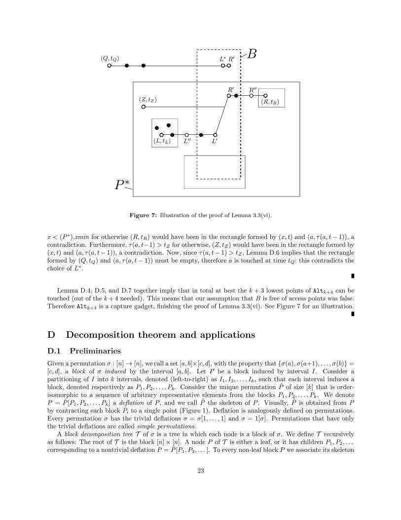
Figure 7: Illustration of the proof of Lemma 3.3(vi).

x < (P ∗).xmin for otherwise (R, tR) would have been in the rectangle formed by (x, t) and (a, τ(a, t− 1)), acontradiction. Furthermore, τ(a, t−1) > tZ for otherwise, (Z, tZ) would have been in the rectangle formed by(x, t) and (a, τ(a, t− 1)), a contradiction. Now, since τ(a, t− 1) > tZ , Lemma D.6 implies that the rectangleformed by (Q, tQ) and (a, τ(a, t− 1)) must be empty, therefore a is touched at time tQ; this contradicts thechoice of L∗.

Lemma D.4, D.5, and D.7 together imply that in total at best the k + 3 lowest points of Altk+4 can betouched (out of the k+ 4 needed). This means that our assumption that B is free of access points was false.Therefore Altk+4 is a capture gadget, finishing the proof of Lemma 3.3(vi). See Figure 7 for an illustration.

D Decomposition theorem and applications

D.1 Preliminaries

Given a permutation σ : [n]→ [n], we call a set [a, b]×[c, d], with the property that σ(a), σ(a+1), . . . , σ(b) =[c, d], a block of σ induced by the interval [a, b]. Let P be a block induced by interval I. Consider apartitioning of I into k intervals, denoted (left-to-right) as I1, I2, . . . , Ik, such that each interval induces ablock, denoted respectively as P1, P2, . . . , Pk. Consider the unique permutation P of size [k] that is order-isomorphic to a sequence of arbitrary representative elements from the blocks P1, P2, . . . , Pk. We denoteP = P [P1, P2, . . . , Pk] a deflation of P , and we call P the skeleton of P . Visually, P is obtained from Pby contracting each block Pi to a single point (Figure 1). Deflation is analogously defined on permutations.Every permutation σ has the trivial deflations σ = σ[1, . . . , 1] and σ = 1[σ]. Permutations that have onlythe trivial deflations are called simple permutations.

A block decomposition tree T of σ is a tree in which each node is a block of σ. We define T recursivelyas follows: The root of T is the block [n]× [n]. A node P of T is either a leaf, or it has children P1, P2, . . .corresponding to a nontrivial deflation P = P [P1, P2, . . . ]. To every non-leaf block P we associate its skeleton

23

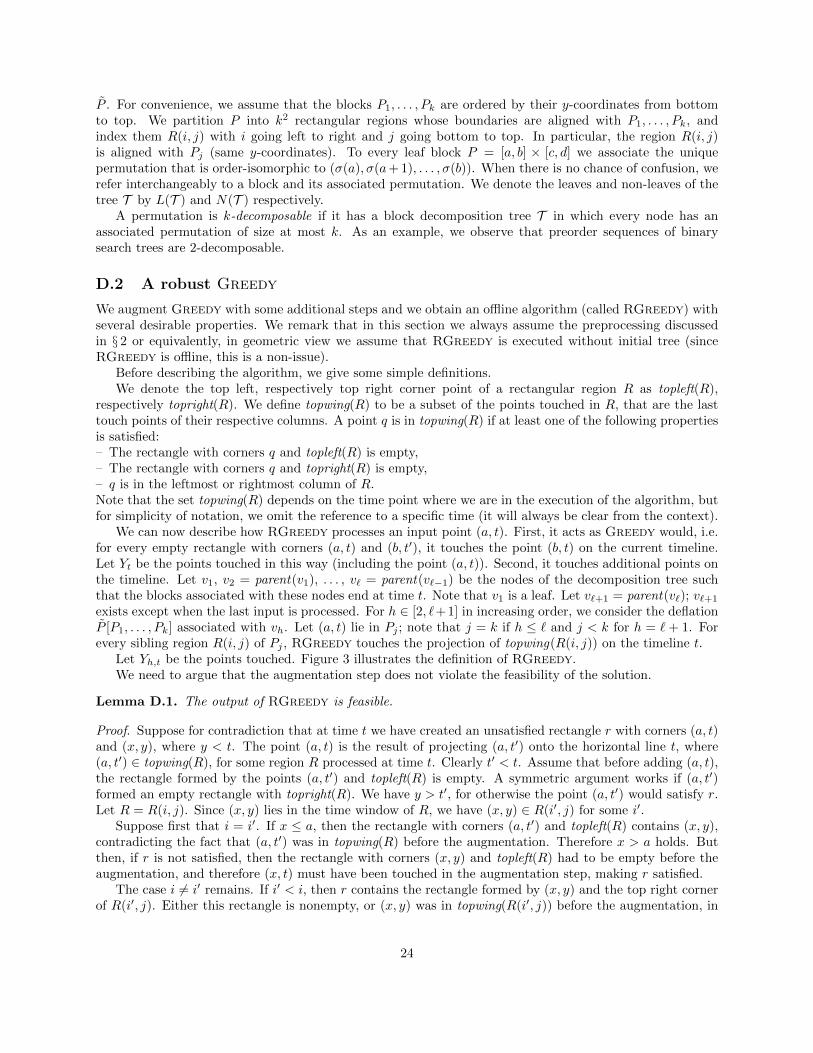
P . For convenience, we assume that the blocks P1, . . . , Pk are ordered by their y-coordinates from bottomto top. We partition P into k2 rectangular regions whose boundaries are aligned with P1, . . . , Pk, andindex them R(i, j) with i going left to right and j going bottom to top. In particular, the region R(i, j)is aligned with Pj (same y-coordinates). To every leaf block P = [a, b] × [c, d] we associate the uniquepermutation that is order-isomorphic to (σ(a), σ(a+ 1), . . . , σ(b)). When there is no chance of confusion, werefer interchangeably to a block and its associated permutation. We denote the leaves and non-leaves of thetree T by L(T ) and N(T ) respectively.

A permutation is k-decomposable if it has a block decomposition tree T in which every node has anassociated permutation of size at most k. As an example, we observe that preorder sequences of binarysearch trees are 2-decomposable.

D.2 A robust Greedy

We augment Greedy with some additional steps and we obtain an offline algorithm (called RGreedy) withseveral desirable properties. We remark that in this section we always assume the preprocessing discussedin § 2 or equivalently, in geometric view we assume that RGreedy is executed without initial tree (sinceRGreedy is offline, this is a non-issue).

Before describing the algorithm, we give some simple definitions.We denote the top left, respectively top right corner point of a rectangular region R as topleft(R),

respectively topright(R). We define topwing(R) to be a subset of the points touched in R, that are the lasttouch points of their respective columns. A point q is in topwing(R) if at least one of the following propertiesis satisfied:– The rectangle with corners q and topleft(R) is empty,– The rectangle with corners q and topright(R) is empty,– q is in the leftmost or rightmost column of R.Note that the set topwing(R) depends on the time point where we are in the execution of the algorithm, butfor simplicity of notation, we omit the reference to a specific time (it will always be clear from the context).

We can now describe how RGreedy processes an input point (a, t). First, it acts as Greedy would, i.e.for every empty rectangle with corners (a, t) and (b, t′), it touches the point (b, t) on the current timeline.Let Yt be the points touched in this way (including the point (a, t)). Second, it touches additional points onthe timeline. Let v1, v2 = parent(v1), . . . , v` = parent(v`−1) be the nodes of the decomposition tree suchthat the blocks associated with these nodes end at time t. Note that v1 is a leaf. Let v`+1 = parent(v`); v`+1

exists except when the last input is processed. For h ∈ [2, `+1] in increasing order, we consider the deflationP [P1, . . . , Pk] associated with vh. Let (a, t) lie in Pj ; note that j = k if h ≤ ` and j < k for h = ` + 1. Forevery sibling region R(i, j) of Pj , RGreedy touches the projection of topwing(R(i, j)) on the timeline t.

Let Yh,t be the points touched. Figure 3 illustrates the definition of RGreedy.We need to argue that the augmentation step does not violate the feasibility of the solution.

Lemma D.1. The output of RGreedy is feasible.

Proof. Suppose for contradiction that at time t we have created an unsatisfied rectangle r with corners (a, t)and (x, y), where y < t. The point (a, t) is the result of projecting (a, t′) onto the horizontal line t, where(a, t′) ∈ topwing(R), for some region R processed at time t. Clearly t′ < t. Assume that before adding (a, t),the rectangle formed by the points (a, t′) and topleft(R) is empty. A symmetric argument works if (a, t′)formed an empty rectangle with topright(R). We have y > t′, for otherwise the point (a, t′) would satisfy r.Let R = R(i, j). Since (x, y) lies in the time window of R, we have (x, y) ∈ R(i′, j) for some i′.

Suppose first that i = i′. If x ≤ a, then the rectangle with corners (a, t′) and topleft(R) contains (x, y),contradicting the fact that (a, t′) was in topwing(R) before the augmentation. Therefore x > a holds. Butthen, if r is not satisfied, then the rectangle with corners (x, y) and topleft(R) had to be empty before theaugmentation, and therefore (x, t) must have been touched in the augmentation step, making r satisfied.

The case i 6= i′ remains. If i′ < i, then r contains the rectangle formed by (x, y) and the top right cornerof R(i′, j). Either this rectangle is nonempty, or (x, y) was in topwing(R(i′, j)) before the augmentation, in

24

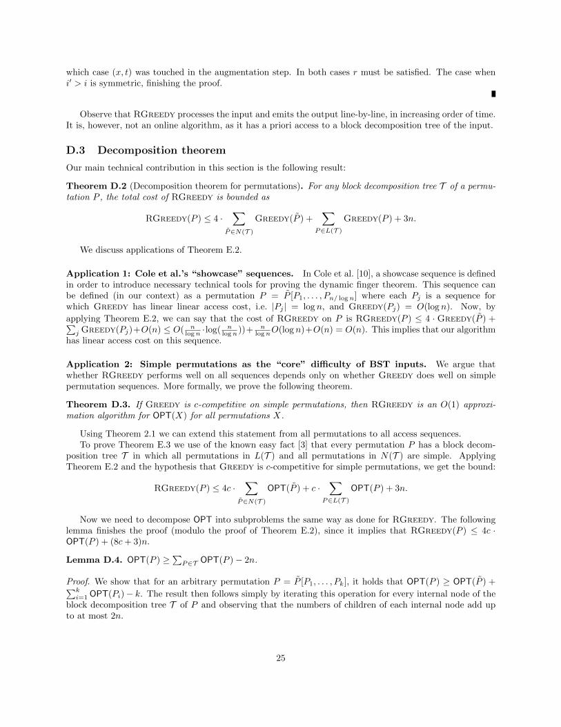
which case (x, t) was touched in the augmentation step. In both cases r must be satisfied. The case wheni′ > i is symmetric, finishing the proof.

Observe that RGreedy processes the input and emits the output line-by-line, in increasing order of time.It is, however, not an online algorithm, as it has a priori access to a block decomposition tree of the input.

D.3 Decomposition theorem

Our main technical contribution in this section is the following result:

Theorem D.2 (Decomposition theorem for permutations). For any block decomposition tree T of a permu-tation P , the total cost of RGreedy is bounded as

RGreedy(P ) ≤ 4 ·∑

P∈N(T )

Greedy(P ) +∑

P∈L(T )

Greedy(P ) + 3n.

We discuss applications of Theorem E.2.

Application 1: Cole et al.’s “showcase” sequences. In Cole et al. [10], a showcase sequence is definedin order to introduce necessary technical tools for proving the dynamic finger theorem. This sequence canbe defined (in our context) as a permutation P = P [P1, . . . , Pn/ logn] where each Pj is a sequence forwhich Greedy has linear linear access cost, i.e. |Pj | = log n, and Greedy(Pj) = O(log n). Now, by

applying Theorem E.2, we can say that the cost of RGreedy on P is RGreedy(P ) ≤ 4 · Greedy(P ) +∑j Greedy(Pj)+O(n) ≤ O( n

logn · log( nlogn ))+ n

lognO(log n)+O(n) = O(n). This implies that our algorithmhas linear access cost on this sequence.

Application 2: Simple permutations as the “core” difficulty of BST inputs. We argue thatwhether RGreedy performs well on all sequences depends only on whether Greedy does well on simplepermutation sequences. More formally, we prove the following theorem.

Theorem D.3. If Greedy is c-competitive on simple permutations, then RGreedy is an O(1) approxi-mation algorithm for OPT(X) for all permutations X.

Using Theorem 2.1 we can extend this statement from all permutations to all access sequences.To prove Theorem E.3 we use of the known easy fact [3] that every permutation P has a block decom-

position tree T in which all permutations in L(T ) and all permutations in N(T ) are simple. ApplyingTheorem E.2 and the hypothesis that Greedy is c-competitive for simple permutations, we get the bound:

RGreedy(P ) ≤ 4c ·∑

P∈N(T )

OPT(P ) + c ·∑

P∈L(T )

OPT(P ) + 3n.

Now we need to decompose OPT into subproblems the same way as done for RGreedy. The followinglemma finishes the proof (modulo the proof of Theorem E.2), since it implies that RGreedy(P ) ≤ 4c ·OPT(P ) + (8c+ 3)n.

Lemma D.4. OPT(P ) ≥∑P∈T OPT(P )− 2n.

Proof. We show that for an arbitrary permutation P = P [P1, . . . , Pk], it holds that OPT(P ) ≥ OPT(P ) +∑ki=1 OPT(Pi)− k. The result then follows simply by iterating this operation for every internal node of the

block decomposition tree T of P and observing that the numbers of children of each internal node add upto at most 2n.

25

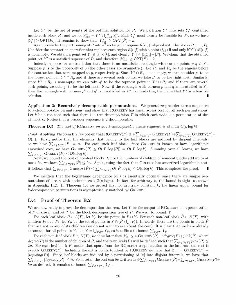
Let Y ∗ be the set of points of the optimal solution for P . We partition Y ∗ into sets Y ∗i contained

inside each block Pi, and we let Y ∗out = Y ∗ \⋃ki=1 Y

∗i . Each Y ∗i must clearly be feasible for Pi, so we have

|Y ∗i | ≥ OPT(Pi). It remains to show that |Y ∗out| ≥ OPT (P )− k.Again, consider the partitioning of P into k2 rectangular regionsR(i, j), aligned with the blocks P1, . . . , Pk.

Consider the contraction operation that replaces each regionR(i, j) with a point (i, j) if and only if Y ∗∩R(i, j)is nonempty. We obtain a point set Y ′ ∈ [k]× [k], and clearly |Y ′| ≤ |Y ∗out|+ |P |. We claim that the obtainedpoint set Y ′ is a satisfied superset of P , and therefore |Y ∗out| ≥ OPT(P )− k.

Indeed, suppose for contradiction that there is an unsatisfied rectangle with corner points p, q ∈ Y ′.Suppose p is to the upper-left of q (the other cases are symmetric). Let Rp and Rq be the regions beforethe contraction that were mapped to p, respectively q. Since Y ∗ ∩Rp is nonempty, we can consider p′ to bethe lowest point in Y ∗ ∩ Rp and if there are several such points, we take p′ to be the rightmost. Similarly,since Y ∗ ∩ Rq is nonempty, we can take q′ to be the topmost point in Y ∗ ∩ Rq and if there are severalsuch points, we take q′ to be the leftmost. Now, if the rectangle with corners p and q is unsatisfied in Y ′,then the rectangle with corners p′ and q′ is unsatisfied in Y ∗, contradicting the claim that Y ∗ is a feasiblesolution.

Application 3: Recursively decomposable permutations. We generalize preorder access sequencesto k-decomposable permutations, and show that RGreedy has linear access cost for all such permutations.Let k be a constant such that there is a tree decomposition T in which each node is a permutation of sizeat most k. Notice that a preorder sequence is 2-decomposable.

Theorem D.5. The cost of RGreedy on any k-decomposable access sequence is at most O(n log k).

Proof. Applying Theorem E.2, we obtain that RGreedy(P ) ≤ 4∑P∈N(T ) Greedy(P )+

∑P∈L(T ) Greedy(P )+

O(n). First, notice that the elements that belong to the leaf blocks are induced by disjoint intervals,so we have

∑P∈L(T ) |P | = n. For each such leaf block, since Greedy is known to have logarithmic

amortized cost, we have Greedy(P ) ≤ O(|P | log |P |) = O(|P | log k). Summing over all leaves, we have∑P∈L(T ) Greedy(P ) ≤ O(n log k).Next, we bound the cost of non-leaf blocks. Since the numbers of children of non-leaf blocks add up to at

most 2n, we have∑P∈N(T ) |P | ≤ 2n. Again, using the fact that Greedy has amortized logarithmic cost,

it follows that∑P∈N(T ) Greedy(P ) ≤

∑P∈N(T )O(|P | log k) ≤ O(n log k). This completes the proof.

We mention that the logarithmic dependence on k is essentially optimal, since there are simple per-mutations of size n with optimum cost Ω(n log n). In fact, for arbitrary k, the bound is tight, as shownin Appendix H.2. In Theorem 1.4 we proved that for arbitrary constant k, the linear upper bound fork-decomposable permutations is asymptotically matched by Greedy.

D.4 Proof of Theorem E.2

We are now ready to prove the decomposition theorem. Let Y be the output of RGreedy on a permutationof P of size n, and let T be the block decomposition tree of P . We wish to bound |Y |.

For each leaf block P ∈ L(T ), let YP be the points in P ∩ Y . For each non-leaf block P ∈ N(T ), withchildren P1, . . . , Pk, let YP be the set of points in Y ∩ (P \

⋃j Pj). In words, these are the points in block P

that are not in any of its children (we do not want to overcount the cost). It is clear that we have alreadyaccounted for all points in Y , i.e. Y =

⋃P∈T YP , so it suffices to bound

∑P∈T |YP |.

For each non-leaf block P ∈ N(T ), we show later that |YP | ≤ 4·Greedy(P )+5degree(P )+junk(P ), where

degree(P ) is the number of children of P , and the term junk(P ) will be defined such that∑P∈N(T ) junk(P ) ≤

2n. For each leaf block P , notice that apart from the RGreedy augmentation in the last row, the cost isexactly Greedy(P ). Including the extra points touched by RGreedy we have that |YP | = Greedy(P ) +|topwing(P )|. Since leaf blocks are induced by a partitioning of [n] into disjoint intervals, we have that∑P∈L(T ) |topwing(P )| ≤ n. So in total, the cost can be written as 4·

∑P∈N(T ) Greedy(P )+

∑P∈L(T ) Greedy(P )+

5n as desired. It remains to bound∑P∈N(T ) |YP |.

26

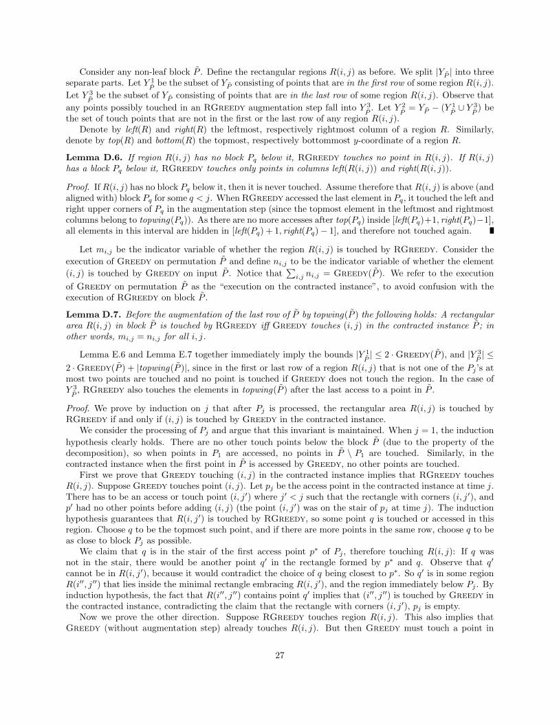
Consider any non-leaf block P . Define the rectangular regions R(i, j) as before. We split |YP | into threeseparate parts. Let Y 1

Pbe the subset of YP consisting of points that are in the first row of some region R(i, j).

Let Y 3P

be the subset of YP consisting of points that are in the last row of some region R(i, j). Observe that

any points possibly touched in an RGreedy augmentation step fall into Y 3P

. Let Y 2P

= YP − (Y 1P∪ Y 3

P) be

the set of touch points that are not in the first or the last row of any region R(i, j).Denote by left(R) and right(R) the leftmost, respectively rightmost column of a region R. Similarly,

denote by top(R) and bottom(R) the topmost, respectively bottommost y-coordinate of a region R.

Lemma D.6. If region R(i, j) has no block Pq below it, RGreedy touches no point in R(i, j). If R(i, j)has a block Pq below it, RGreedy touches only points in columns left(R(i, j)) and right(R(i, j)).

Proof. If R(i, j) has no block Pq below it, then it is never touched. Assume therefore that R(i, j) is above (andaligned with) block Pq for some q < j. When RGreedy accessed the last element in Pq, it touched the left andright upper corners of Pq in the augmentation step (since the topmost element in the leftmost and rightmostcolumns belong to topwing(Pq)). As there are no more accesses after top(Pq) inside [left(Pq)+1, right(Pq)−1],all elements in this interval are hidden in [left(Pq) + 1, right(Pq)− 1], and therefore not touched again.

Let mi,j be the indicator variable of whether the region R(i, j) is touched by RGreedy. Consider the

execution of Greedy on permutation P and define ni,j to be the indicator variable of whether the element

(i, j) is touched by Greedy on input P . Notice that∑i,j ni,j = Greedy(P ). We refer to the execution

of Greedy on permutation P as the “execution on the contracted instance”, to avoid confusion with theexecution of RGreedy on block P .

Lemma D.7. Before the augmentation of the last row of P by topwing(P ) the following holds: A rectangulararea R(i, j) in block P is touched by RGreedy iff Greedy touches (i, j) in the contracted instance P ; inother words, mi,j = ni,j for all i, j.

Lemma E.6 and Lemma E.7 together immediately imply the bounds |Y 1P| ≤ 2 ·Greedy(P ), and |Y 3

P| ≤

2 ·Greedy(P ) + |topwing(P )|, since in the first or last row of a region R(i, j) that is not one of the Pj ’s atmost two points are touched and no point is touched if Greedy does not touch the region. In the case ofY 3P

, RGreedy also touches the elements in topwing(P ) after the last access to a point in P .

Proof. We prove by induction on j that after Pj is processed, the rectangular area R(i, j) is touched byRGreedy if and only if (i, j) is touched by Greedy in the contracted instance.

We consider the processing of Pj and argue that this invariant is maintained. When j = 1, the induction

hypothesis clearly holds. There are no other touch points below the block P (due to the property of thedecomposition), so when points in P1 are accessed, no points in P \ P1 are touched. Similarly, in thecontracted instance when the first point in P is accessed by Greedy, no other points are touched.

First we prove that Greedy touching (i, j) in the contracted instance implies that RGreedy touchesR(i, j). Suppose Greedy touches point (i, j). Let pj be the access point in the contracted instance at time j.There has to be an access or touch point (i, j′) where j′ < j such that the rectangle with corners (i, j′), andp′ had no other points before adding (i, j) (the point (i, j′) was on the stair of pj at time j). The inductionhypothesis guarantees that R(i, j′) is touched by RGreedy, so some point q is touched or accessed in thisregion. Choose q to be the topmost such point, and if there are more points in the same row, choose q to beas close to block Pj as possible.

We claim that q is in the stair of the first access point p∗ of Pj , therefore touching R(i, j): If q wasnot in the stair, there would be another point q′ in the rectangle formed by p∗ and q. Observe that q′

cannot be in R(i, j′), because it would contradict the choice of q being closest to p∗. So q′ is in some regionR(i′′, j′′) that lies inside the minimal rectangle embracing R(i, j′), and the region immediately below Pj . Byinduction hypothesis, the fact that R(i′′, j′′) contains point q′ implies that (i′′, j′′) is touched by Greedy inthe contracted instance, contradicting the claim that the rectangle with corners (i, j′), pj is empty.

Now we prove the other direction. Suppose RGreedy touches region R(i, j). This also implies thatGreedy (without augmentation step) already touches R(i, j). But then Greedy must touch a point in

27

R(i, j) when accessing the first element p∗ in Pj . Assume w.l.o.g. that R(i, j) is to the right of Pj . Itmeans that there is a point q in the stair of p∗, such that q is in some region R(i, j′) for j′ < j. If in thecontracted instance (i, j′) is in the stair of the access point pj at time j, we would be done (because Greedywould add point (i, j)), so asssume otherwise that this is not the case. Let (i′′, j′′) be the point that blocks(i, j′), so the corresponding region R(i′′, j′′) lies inside the minimal rectangle embracing both Pj and R(i, j′).

Also note that the region R(i′′, j′′) cannot be vertically aligned with Pj because P is a permutation. Thusi < i′′. The fact that (i′′, j′′) is touched by Greedy implies, by induction hypothesis, the existence of apoint q′ ∈ R(i′′, j′′), and therefore the augmentation step of RGreedy touches some point q∗ on the toprow of region R(i′′, j′′). This point would prevent q from being on the stair of p∗, a contradiction.

Lemma D.8. |topwing(P )| ≤ 2 · degree(P ).

Proof. topwing(P ) contains at most 2 points in block R(i, k) for every k.

The only task left is to bound |Y 2P|, the number of touch points in non-first and non-last rows of a region.

This will be the junk term mentioned earlier, that sums to 2n over all blocks P ∈ N(T ). In particular weshow that every access point can contribute at most 2 to the entire sum

∑P∈N(T ) |Y 2

P|.

Consider any access point X = (x, tx), and let P ∗ denote the smallest block that contains X, and in whichX is not the first access point (such a block exists for all but the very first access point of the input). Furtherobserve, that every point touched at time tx inside P ∗ is accounted for already in the sum

∑P∈N(T ) |Y 1

P|,

since these points are in the first row of some region inside P ∗. It remains to show that at time tx at mosttwo points are touched outside of P ∗, excluding a possible RGreedy augmentation step (which we alreadyaccounted for). Let p∗ denote the first access point in P ∗, i.e. at time bottom(P ∗). At the time of accessingp∗ several points might be touched. Notice that all these points must be outside of P ∗, since no elementis touched before being accessed. Let pleft and pright be the nearest of these touch points to p∗ on its left,respectively on its right.

We claim that for all the access points in P ∗ other than the first access point p∗, only pleft and pright canbe touched outside of P ∗. Since, by definition X is a non-first element of P ∗, it follows that at time tx atmost two points are touched outside of P ∗, exactly what we wish to prove.

Indeed, elements in the interval [1, pleft − 1], and in the interval [pright + 1, n] are hidden in [1, pleft − 1],respectively in [pright + 1, n], in the time interval [bottom(P ∗) + 1, top(P ∗)] and therefore cannot be touchedwhen accessing non-first elements in P ∗. The case remains when pleft or pright or both are nonexistent. Inthis case it is easy to see that if on the corresponding side an element outside of P ∗ were to be touched atthe time of a non-first access in P ∗, then it would have had to be touched at the time of p∗, a contradiction.

This concludes the proof.

E Proof of Theorem 2.1

In this section, we prove the following theorem.

Theorem E.1 (Theorem 2.1). Assume that there is a c-competitive online geometric BST Ap for all per-mutations. Then there is a 4c-competitive online geometric BST A for all access sequences.

Given a c-competitive online BST Ap that can serve a permutation access sequence, we construct a4c-competitive online BST A that can serve any (not necessarily permutation) access sequences. We firstsketch the outline of the proof.

Let X ∈ [n]m be a (possibly non-permutation) access sequence, and let T be the initial tree on [n]. Firstwe show that given any online BST B that can handle accesses, there is a canonical way to augment B andobtain an augmented Bins , that can also handle insertions of elements.

Then, we show that given any access-only sequence X ∈ [n]m, initial tree T and an online augmentedBST Ap,ins that can serve permutation access and insert sequences, we can construct a permutation sequence(comprising of both accesses and insertions) Xp,ins ∈ [m]m to be fed to Ap,ins in an online manner. Then

28

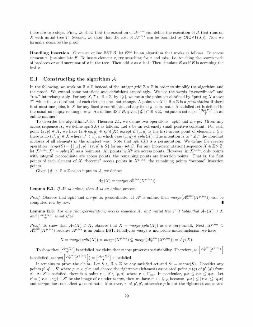
there are two steps. First, we show that the execution of Ap,ins can define the execution of A that runs onX with initial tree T . Second, we show that the cost of Ap,ins can be bounded by O(OPT(X)). Now weformally describe the proof.

Handling Insertion Given an online BST B, let Bins be an algorithm that works as follows. To accesselement x, just simulate B. To insert element x, try searching for x and miss, i.e. touching the search pathof predecessor and successor of x in the tree. Then add x as a leaf. Then simulate B as if B is accessing theleaf x.

E.1 Constructing the algorithm AIn the following, we work on R× Z instead of the integer grid Z× Z in order to simplify the algorithm andthe proof. We extend some notations and definitions accordingly. We use the words “y-coordinate” and“row” interchangeably. For any X,T ⊂ R×Z, by [XT ], we mean the point set obtained by “putting X aboveT” while the x-coordinate of each element does not change. A point set X ⊂ R×Z is a permutation if thereis at most one point in X for any fixed x-coordinate and any fixed y-coordinate. A satisfied set is defined inthe usual no-empty-rectangle way. An online BST B, given [XT ] ⊂ R× Z, outputs a satisfied

[ BT (X)T

]in an

online manner.To describe the algorithm A for Theorem 2.1, we define two operations: split and merge. Given any

access sequence X, we define split(X) as follows. Let ε be an extremely small positive constant. For eachpoint (x, y) ∈ X, we have (x + εy, y) ∈ split(X) except if (x, y) is the first access point of element x (i.e.there is no (x′, y) ∈ X where x′ < x), in which case (x, y) ∈ split(X). The intention is to “tilt” the non-firstaccesses of all elements in the simplest way. Note that split(X) is a permutation. We define the reverseoperation merge(S) = (bxc , y) | (x, y) ∈ S for any set S. For any (non-permutation) sequence X ∈ Z×Z,let Xp,ins , Xp = split(X) as a point set. All points in Xp are access points. However, in Xp,ins , only pointswith integral x-coordinate are access points, the remaining points are insertion points. That is, the firstpoints of each element of X “become” access points in Xp,ins , the remaining points “become” insertionpoints.

Given [XT ] ∈ Z× Z as an input to A, we define:

AT (X) = merge(Ap,insT (Xp,ins))

Lemma E.2. If Ap is online, then A is an online process.

Proof. Observe that split and merge fix y-coordinate. If Ap is online, then merge(Ap,insT (Xp,ins)) can becomputed row by row.

Lemma E.3. For any (non-permutation) access sequence X, and initial tree T it holds that AT (X) ⊇ Xand

[AT (X)T

]is satisfied

Proof. To show that AT (X) ⊇ X, observe that X = merge(split(X)) as ε is very small. Next, Xp,ins ⊆Ap,insT (Xp,ins) because Ap,ins is an online BST. Finally, as merge is monotone under inclusion, we have

X = merge(split(X)) = merge(Xp,ins) ⊆ merge(Ap,insT (Xp,ins)) = AT (X).

To show that[AT (X)

T

]is satisfied, we claim that merge preserves satisfiability. Therefore, as

[Ap,insT (Xp,ins)

T

]is satisfied, merge(

[Ap,insT (Xp,ins)

T

]) =

[AT (X)T

]is satisfied.

It remains to prove the claim. Let S ⊂ R × Z be any satisfied set and S′ = merge(S). Consider anypoints p′, q′ ∈ S′ where p′.x < q′.x and choose the rightmost (leftmost) associated point p (q) of p′ (q′) fromS. As S is satisfied, there is a point r ∈ S \ p, q where r ∈ pq. In particular, p.x ≤ r.x ≤ q.x. Letr′ = (br.xc , r.y) ∈ S′ be the image of r under merge, then we have r′ ∈ p′q′ because bp.xc ≤ br.xc ≤ bq.xcand merge does not affect y-coordinate. Moreover, r′ 6= p′, q′, otherwise p is not the rightmost associated

29

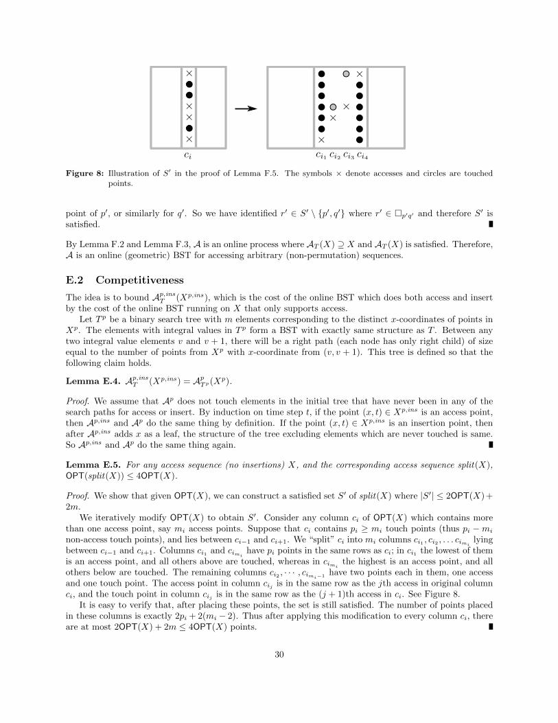
Figure 8: Illustration of S′ in the proof of Lemma F.5. The symbols × denote accesses and circles are touchedpoints.

point of p′, or similarly for q′. So we have identified r′ ∈ S′ \ p′, q′ where r′ ∈ p′q′ and therefore S′ issatisfied.

By Lemma F.2 and Lemma F.3, A is an online process where AT (X) ⊇ X and AT (X) is satisfied. Therefore,A is an online (geometric) BST for accessing arbitrary (non-permutation) sequences.

E.2 Competitiveness

The idea is to bound Ap,insT (Xp,ins), which is the cost of the online BST which does both access and insertby the cost of the online BST running on X that only supports access.

Let T p be a binary search tree with m elements corresponding to the distinct x-coordinates of points inXp. The elements with integral values in T p form a BST with exactly same structure as T . Between anytwo integral value elements v and v + 1, there will be a right path (each node has only right child) of sizeequal to the number of points from Xp with x-coordinate from (v, v + 1). This tree is defined so that thefollowing claim holds.

Lemma E.4. Ap,insT (Xp,ins) = ApTp(Xp).

Proof. We assume that Ap does not touch elements in the initial tree that have never been in any of thesearch paths for access or insert. By induction on time step t, if the point (x, t) ∈ Xp,ins is an access point,then Ap,ins and Ap do the same thing by definition. If the point (x, t) ∈ Xp,ins is an insertion point, thenafter Ap,ins adds x as a leaf, the structure of the tree excluding elements which are never touched is same.So Ap,ins and Ap do the same thing again.

Lemma E.5. For any access sequence (no insertions) X, and the corresponding access sequence split(X),OPT(split(X)) ≤ 4OPT(X).

Proof. We show that given OPT(X), we can construct a satisfied set S′ of split(X) where |S′| ≤ 2OPT(X)+2m.

We iteratively modify OPT(X) to obtain S′. Consider any column ci of OPT(X) which contains morethan one access point, say mi access points. Suppose that ci contains pi ≥ mi touch points (thus pi −mi

non-access touch points), and lies between ci−1 and ci+1. We “split” ci into mi columns ci1 , ci2 , . . . cimi lyingbetween ci−1 and ci+1. Columns ci1 and cimi have pi points in the same rows as ci; in ci1 the lowest of themis an access point, and all others above are touched, whereas in cimi the highest is an access point, and allothers below are touched. The remaining columns ci2 , · · · , cimi−1 have two points each in them, one accessand one touch point. The access point in column cij is in the same row as the jth access in original columnci, and the touch point in column cij is in the same row as the (j + 1)th access in ci. See Figure 8.

It is easy to verify that, after placing these points, the set is still satisfied. The number of points placedin these columns is exactly 2pi + 2(mi − 2). Thus after applying this modification to every column ci, thereare at most 2OPT(X) + 2m ≤ 4OPT(X) points.

30

Now we are ready to prove the main theorem.Proof of Theorem 2.1. First, we have that AT (X) ≤ Ap,insT (Xp,ins) because merge never increases thenumber of points. We conclude that

AT (X) ≤ Ap,insT (Xp,ins) = ApTp(Xp) ≤ cOPT(split(X)) ≤ 4cOPT(X),

where the second inequality follows from Lemma F.4, the third inequality follows from the assumption thatAp is c-competitive for only accessing on only permutations, and the last inequality follows from Lemma F.5,and hence A is a 4c-competitive online BST for any access sequence.

F Random permutation is hard

We prove that the cost of most permutations is Ω(n log n) for all BST algorithm. A similar result has beenshown by Wilber [39] for random access sequences (that might not be permutations). More formally, weprove the following theorem.

Theorem F.1. There is a positive constant c such that for any L > 0 only a fraction 1/2L of the permutationsX have OPT(X) ≤ (log n!− L− n− 1)/c.

Proof. We use Kolmogorov complexity. Observe that the shape of a tree on k nodes can be encoded by O(k)bits, e.g., by the preorder traversal. If the keys stored in the tree are clear from the context, the assignmentof the keys to the nodes is unique. Let T be the initial tree, let X be any (permutation) access sequence,and let CX be the total cost of OPT on X. We encode the shape of the initial tree with O(n) bits. Considernow an access of cost k. It replaces an initial segment of the current search tree, the before-tree, by anothertree on the same set of nodes, the after-tree. The before-tree must include the element accessed and has sizeO(k). We encode the before-tree and the after-tree with O(k) bits and use a special marker to designatethe accessed element in the before-tree. In total, we need c · (n+ CX) bits for the encoding for some smallconstant c. Note that X can be reconstructed from the encoding. We first reconstruct the shape of the initialtree. Its labelling by keys is unique. Consider now any access. Since the position of the accessed elementin the before-tree is marked and since the before- and the after-tree are on the same set of keys, the searchtree after the access is determined. We conclude that we have an injective mapping from permutations Xto bitstrings of length c · (n + CX). Assume Cx ≤ (log n! − L − n − 1)/c. Then the encoding of X has atmost log n!− L− 1 bits and hence X is in a set of at most n!/2L permutations.

G Other claims

G.1 Counterexamples for straightforward attempts

Avoiding the same pattern is not enough.

It might be tempting to conjecture that if X avoids P , then the Greedy touch matrix Greedy(X) avoidsP as well (P refers both to a permutation pattern and its matrix representation). While this holds for thesimple case P = (2, 3, 1) in the “no initial tree”-case (proof left as an exercise for the reader), in general itis not true. Figure 9 shows a counterexample (P = (3, 2, 1)).

Greedy is not decomposable.

One could prove a decomposition theorem similar to Theorem E.2 for Greedy, if Greedy were decomposable.By this we mean that for a k-decomposable input sequence, considering a certain level P = P [P1, . . . , Pk]of the decomposition tree, Greedy touches a region R(i, j), iff the corresponding point (i, j) is touched byGreedy, when executed on the contracted instance P . Alas, this property does not hold for Greedy, asshown on Figure 10.

31

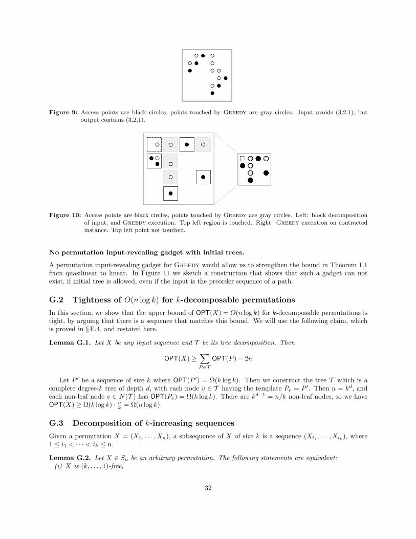
Figure 9: Access points are black circles, points touched by Greedy are gray circles. Input avoids (3,2,1), butoutput contains (3,2,1).

Figure 10: Access points are black circles, points touched by Greedy are gray circles. Left: block decompositionof input, and Greedy execution. Top left region is touched. Right: Greedy execution on contractedinstance. Top left point not touched.

No permutation input-revealing gadget with initial trees.

A permutation input-revealing gadget for Greedy would allow us to strengthen the bound in Theorem 1.1from quasilinear to linear. In Figure 11 we sketch a construction that shows that such a gadget can notexist, if initial tree is allowed, even if the input is the preorder sequence of a path.

G.2 Tightness of O(n log k) for k-decomposable permutations

In this section, we show that the upper bound of OPT(X) = O(n log k) for k-decomposable permutations istight, by arguing that there is a sequence that matches this bound. We will use the following claim, whichis proved in §E.4, and restated here.

Lemma G.1. Let X be any input sequence and T be its tree decomposition. Then

OPT(X) ≥∑P∈T

OPT(P )− 2n

Let P ′ be a sequence of size k where OPT(P ′) = Ω(k log k). Then we construct the tree T which is acomplete degree-k tree of depth d, with each node v ∈ T having the template Pv = P ′. Then n = kd, andeach non-leaf node v ∈ N(T ) has OPT(Pv) = Ω(k log k). There are kd−1 = n/k non-leaf nodes, so we haveOPT(X) ≥ Ω(k log k) · nk = Ω(n log k).

G.3 Decomposition of k-increasing sequences

Given a permutation X = (X1, . . . , Xn), a subsequence of X of size k is a sequence (Xi1 , . . . , Xik), where1 ≤ i1 < · · · < ik ≤ n.

Lemma G.2. Let X ∈ Sn be an arbitrary permutation. The following statements are equivalent:(i) X is (k, . . . , 1)-free,

32

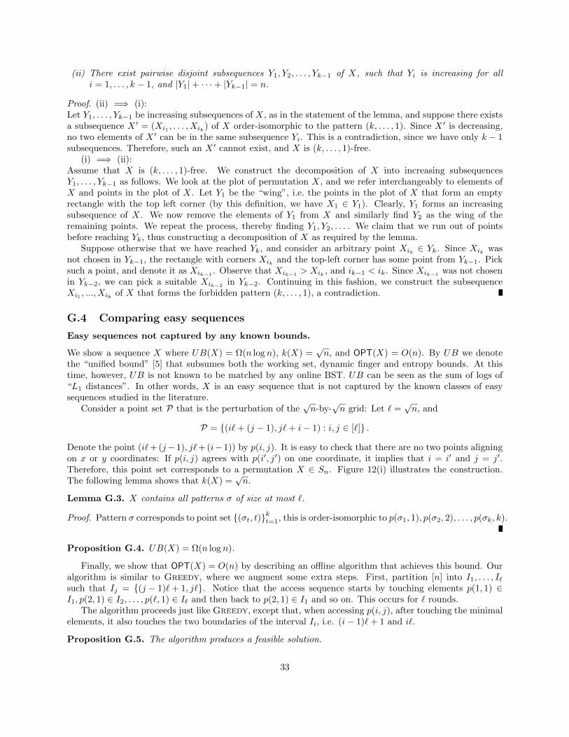
(ii) There exist pairwise disjoint subsequences Y1, Y2, . . . , Yk−1 of X, such that Yi is increasing for alli = 1, . . . , k − 1, and |Y1|+ · · ·+ |Yk−1| = n.

Proof. (ii) =⇒ (i):Let Y1, . . . , Yk−1 be increasing subsequences of X, as in the statement of the lemma, and suppose there existsa subsequence X ′ = (Xi1 , . . . , Xik) of X order-isomorphic to the pattern (k, . . . , 1). Since X ′ is decreasing,no two elements of X ′ can be in the same subsequence Yi. This is a contradiction, since we have only k − 1subsequences. Therefore, such an X ′ cannot exist, and X is (k, . . . , 1)-free.

(i) =⇒ (ii):Assume that X is (k, . . . , 1)-free. We construct the decomposition of X into increasing subsequencesY1, . . . , Yk−1 as follows. We look at the plot of permutation X, and we refer interchangeably to elements ofX and points in the plot of X. Let Y1 be the “wing”, i.e. the points in the plot of X that form an emptyrectangle with the top left corner (by this definition, we have X1 ∈ Y1). Clearly, Y1 forms an increasingsubsequence of X. We now remove the elements of Y1 from X and similarly find Y2 as the wing of theremaining points. We repeat the process, thereby finding Y1, Y2, . . . . We claim that we run out of pointsbefore reaching Yk, thus constructing a decomposition of X as required by the lemma.

Suppose otherwise that we have reached Yk, and consider an arbitrary point Xik ∈ Yk. Since Xik wasnot chosen in Yk−1, the rectangle with corners Xik and the top-left corner has some point from Yk−1. Picksuch a point, and denote it as Xik−1

. Observe that Xik−1> Xik , and ik−1 < ik. Since Xik−1

was not chosenin Yk−2, we can pick a suitable Xik−2

in Yk−2. Continuing in this fashion, we construct the subsequenceXi1 , ..., Xik of X that forms the forbidden pattern (k, . . . , 1), a contradiction.

G.4 Comparing easy sequences

Easy sequences not captured by any known bounds.

We show a sequence X where UB(X) = Ω(n log n), k(X) =√n, and OPT(X) = O(n). By UB we denote

the “unified bound” [5] that subsumes both the working set, dynamic finger and entropy bounds. At thistime, however, UB is not known to be matched by any online BST. UB can be seen as the sum of logs of“L1 distances”. In other words, X is an easy sequence that is not captured by the known classes of easysequences studied in the literature.

Consider a point set P that is the perturbation of the√n-by-

√n grid: Let ` =

√n, and

P = (i`+ (j − 1), j`+ i− 1) : i, j ∈ [`] .

Denote the point (i`+ (j−1), j`+ (i−1)) by p(i, j). It is easy to check that there are no two points aligningon x or y coordinates: If p(i, j) agrees with p(i′, j′) on one coordinate, it implies that i = i′ and j = j′.Therefore, this point set corresponds to a permutation X ∈ Sn. Figure 12(i) illustrates the construction.The following lemma shows that k(X) =

√n.

Lemma G.3. X contains all patterns σ of size at most `.

Proof. Pattern σ corresponds to point set (σt, t)kt=1, this is order-isomorphic to p(σ1, 1), p(σ2, 2), . . . , p(σk, k).

Proposition G.4. UB(X) = Ω(n log n).

Finally, we show that OPT(X) = O(n) by describing an offline algorithm that achieves this bound. Ouralgorithm is similar to Greedy, where we augment some extra steps. First, partition [n] into I1, . . . , I`such that Ij = (j − 1)`+ 1, j`. Notice that the access sequence starts by touching elements p(1, 1) ∈I1, p(2, 1) ∈ I2, . . . , p(`, 1) ∈ I` and then back to p(2, 1) ∈ I1 and so on. This occurs for ` rounds.

The algorithm proceeds just like Greedy, except that, when accessing p(i, j), after touching the minimalelements, it also touches the two boundaries of the interval Ii, i.e. (i− 1)`+ 1 and i`.

Proposition G.5. The algorithm produces a feasible solution.

33

Proposition G.6. The cost of this algorithm is O(n).

A slightly more involved inductive argument shows that Greedy too has linear cost on X.

Proposition G.7. Greedy(X) = O(n).

Pattern avoidance and dynamic finger.

We show examples that k(X) and the dynamic finger bound (denoted by DF (X)) are not comparable.Figure 12(ii) illustrates a sequence X where DF (X) = O(n) and k(X) = Ω(

√n/ log n). First, the sequence

X starts with the perturbed grid construction of size f(n)-by-f(n) where f(n) =√n/ log n; then the sequence

continues with a sequential access of length n − f(n)2. Notice that, in the first phase of the sequence, thedistances between consecutive points are |Xi+1 − Xi| = O(f(n)), except for at most f(n) pairs, whichhave distance O(f(n)2). In the second phase, the distances are one. So DF (X) = O(f(n)2) log f(n) +O(n) = O(n). On the other hand, the f(n)-by-f(n) grid contains all permutations of size f(n), so we havek(X) = Ω(

√n/ log n).

Figure 12(iii) illustrates a 2-recursively decomposable sequence (thus having k(X) = 3) whose dynamicfinger bound is Ω(n log n); to see this, notice that |Xi+1 − Xi| ≥ n/2 for i = 1, . . . , n/2, so we haveDF (X) ≥ n

2 log(n/2).

Easy non-decomposable sequence.

Figure 12(iv) shows the non-decomposable input sequence X = (n/2, n, 1, n − 1, 2, . . . ) on which Greedyachieves linear cost (to see this, observe that Greedy touches at most three elements in each row).

G.5 Why is path the roadblock to deque, traversal, split

The deque-, traversal- and split conjectures are originally stated for splay trees. We first state the conjecturesfor any online BST A.

Conjecture 2 (Deque conjecture [36]). Starting with any initial tree T with n elements, the cost of A forinserting or deleting the current minimum or maximum elements m times is O(m+ n)

Conjecture 3 (Traversal conjecture [34]). Starting with any initial tree T with n elements, the cost ofaccessing a sequence X defined by the preorder sequence of some BST T ′ is O(n).

Conjecture 4 (Split conjecture [26]). Starting with any initial tree T with n elements, the cost of A forsplitting T by any sequence of n splits is O(n). A split at element x is to delete x and to obtain two treeswhose elements are smaller resp. larger than x, each subject to further splittings.

Next, we state an easier conjecture which is implied by all three conjectures.

Conjecture 5 (Path conjecture). Starting with any initial tree T with n elements, the cost of A for accessinga sequence X defined by the preorder sequence of some BST T ′ which is a path is O(n).

To express it in terms of pattern avoidance, the access sequences in the path conjecture avoid both (2, 3, 1)and (2, 1, 3), while the ones in traversal conjecture only avoid (2, 3, 1).

Intuitively, the sequence in path conjecture is a sequence that starts from minimum or maximum andmoves inwards towards the middle, for example, (1, 2, 3, 4, 10, 9, 5, 6, 8, 7).

Theorem G.8. Let A be an online BST.

(i) If A satisfies traversal conjecture, then A satisfies path conjecture.

(ii) If A satisfies deque conjecture, then there is an online BST A′ that satisfies path conjecture.

(iii) If A satisfies split conjecture, then there is an online BST A′ that satisfies path conjecture.

34

Proof. (i) This is clear from the statement.(ii) If A satisfies deque conjecture, then A can delete the current minimum or maximum element n times

with cost O(n). Observe that the sequence of these deletions can be defined by a BST which is a path.Given A, we construct A′ that satisfies path conjecture. To access x = 1 or n, A′ simulates A by deletingx, but then before finishing, A′ brings x back by making x the root.

To access other elements x from the “minimum” (“maximum”) side, A′ also simulates A, but we can seethat it must touch x− 1 (x+ 1) as well. Again, instead of deleting x, A′ makes x as a root. For any time,the cost of A′ is at most the cost of A plus one.

(iii) Splitting is equivalent to deleting when applied to the minimum or maximum element. Thus, if Asatisfies split conjecture, then A satisfies deque conjecture without inserts. We can then use the argumentof (ii).

35

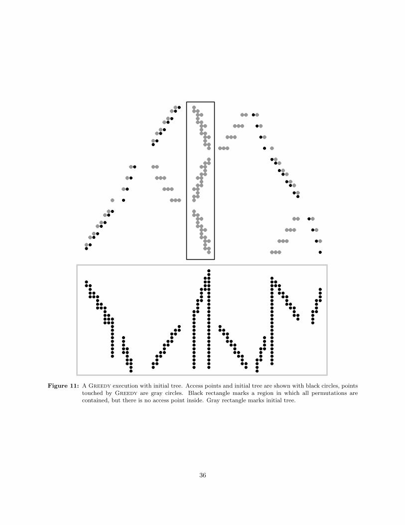
Figure 11: A Greedy execution with initial tree. Access points and initial tree are shown with black circles, pointstouched by Greedy are gray circles. Black rectangle marks a region in which all permutations arecontained, but there is no access point inside. Gray rectangle marks initial tree.

36

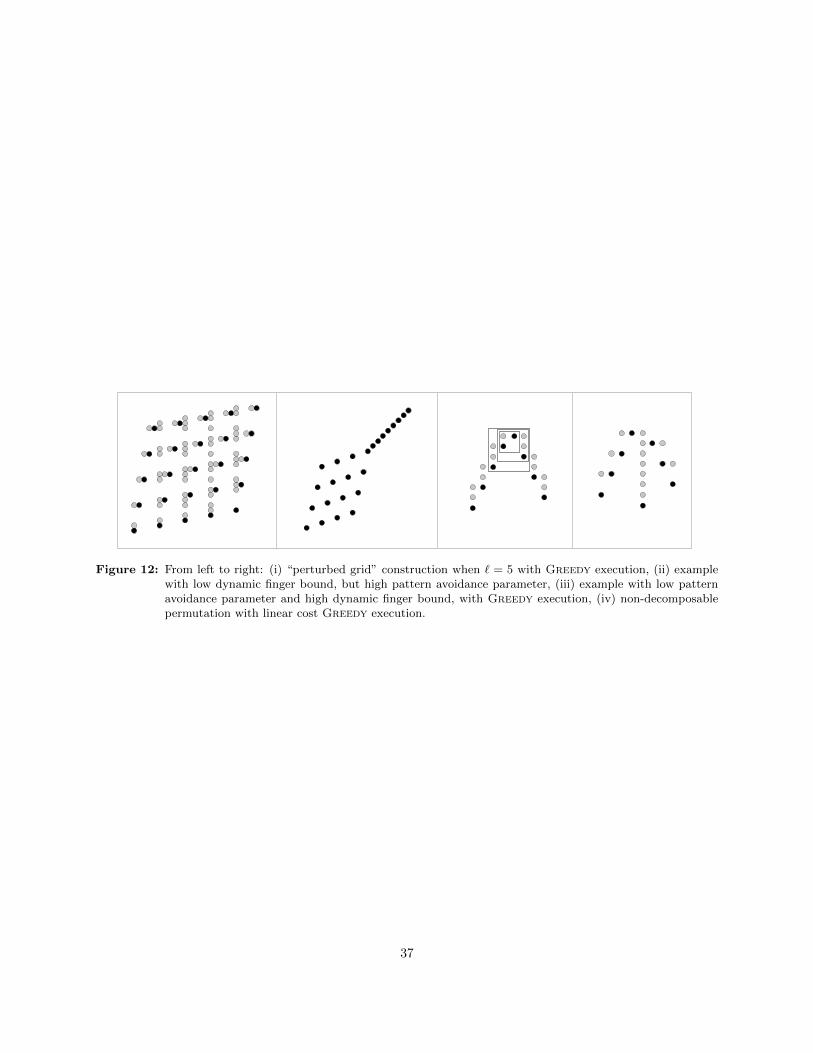
Figure 12: From left to right: (i) “perturbed grid” construction when ` = 5 with Greedy execution, (ii) examplewith low dynamic finger bound, but high pattern avoidance parameter, (iii) example with low patternavoidance parameter and high dynamic finger bound, with Greedy execution, (iv) non-decomposablepermutation with linear cost Greedy execution.

37