Embed Size (px)
Citation preview

Sample Chapter

Pattern Recognition and Machine Learning
Christopher M. Bishop
Copyright c© 2002–2006
This is an extract from the book Pattern Recognition and Machine Learning published by Springer (2006).It contains the preface with details about the mathematicalnotation, the complete table of contents of thebook and an unabridged version of chapter 8 on Graphical Models. This document, as well as furtherinformation about the book, is available from:
http://research.microsoft.com/∼cmbishop/PRML

Preface
Pattern recognition has its origins in engineering, whereas machine learning grewout of computer science. However, these activities can be viewed as two facets ofthe same field, and together they have undergone substantialdevelopment over thepast ten years. In particular, Bayesian methods have grown from a specialist niche tobecome mainstream, while graphical models have emerged as ageneral frameworkfor describing and applying probabilistic models. Also, the practical applicability ofBayesian methods has been greatly enhanced through the development of a range ofapproximate inference algorithms such as variational Bayes and expectation propa-gation. Similarly, new models based on kernels have had significant impact on bothalgorithms and applications.
This new textbook reflects these recent developments while providing a compre-hensive introduction to the fields of pattern recognition and machine learning. It isaimed at advanced undergraduates or first year PhD students,as well as researchersand practitioners, and assumes no previous knowledge of pattern recognition or ma-chine learning concepts. Knowledge of multivariate calculus and basic linear algebrais required, and some familiarity with probabilities wouldbe helpful though not es-sential as the book includes a self-contained introductionto basic probability theory.
Because this book has broad scope, it is impossible to provide a complete list ofreferences, and in particular no attempt has been made to provide accurate historicalattribution of ideas. Instead, the aim has been to give references that offer greaterdetail than is possible here and that hopefully provide entry points into what, in somecases, is a very extensive literature. For this reason, the references are often to morerecent textbooks and review articles rather than to original sources.
The book is supported by a great deal of additional material,including lectureslides as well as the complete set of figures used in the book, and the reader isencouraged to visit the book web site for the latest information:
http://research.microsoft.com/∼cmbishop/PRML
c© Christopher M. Bishop (2002–2006). Springer, 2006. First printing.Further information available athttp://research.microsoft.com/∼cmbishop/PRML
vii
viii PREFACE
ExercisesThe exercises that appear at the end of every chapter form an important com-
ponent of the book. Each exercise has been carefully chosen to reinforce conceptsexplained in the text or to develop and generalize them in significant ways, and eachis graded according to difficulty ranging from(?), which denotes a simple exercisetaking a few minutes to complete, through to(? ? ?), which denotes a significantlymore complex exercise.
It has been difficult to know to what extent worked solutions should be madewidely available. Those engaged in self study will find worked solutions very ben-eficial, whereas many course tutors request that solutions be available only via thepublisher so that the exercises may be used in class. In orderto try to meet theseconflicting requirements, those exercises that help amplify key points in the text, orthat fill in important details, have solutions that are available as a PDF file from thebook web site. Such exercises are denoted bywww . Solutions for the remainingexercises are available to course tutors by contacting the publisher (contact detailsare given on the book web site). Readers are strongly encouraged to work throughthe exercises unaided, and to turn to the solutions only as required.
Although this book focuses on concepts and principles, in a taught course thestudents should ideally have the opportunity to experimentwith some of the keyalgorithms using appropriate data sets. A companion volume(Bishop and Nabney,2008) will deal with practical aspects of pattern recognition and machine learning,and will be accompanied by Matlab software implementing most of the algorithmsdiscussed in this book.
AcknowledgementsFirst of all I would like to express my sincere thanks to Markus Svensen who
has provided immense help with preparation of figures and with the typesetting ofthe book in LATEX. His assistance has been invaluable.
I am very grateful to Microsoft Research for providing a highly stimulating re-search environment and for giving me the freedom to write this book (the views andopinions expressed in this book, however, are my own and are therefore not neces-sarily the same as those of Microsoft or its affiliates).
Springer has provided excellent support throughout the final stages of prepara-tion of this book, and I would like to thank my commissioning editor John Kimmelfor his support and professionalism, as well as Joseph Piliero for his help in design-ing the cover and the text format and MaryAnn Brickner for hernumerous contribu-tions during the production phase. The inspiration for the cover design came from adiscussion with Antonio Criminisi.
I also wish to thank Oxford University Press for permission to reproduce ex-cerpts from an earlier textbook,Neural Networks for Pattern Recognition(Bishop,1995a). The images of the Mark 1 perceptron and of Frank Rosenblatt are repro-duced with the permission of Arvin Calspan Advanced Technology Center. I wouldalso like to thank Asela Gunawardana for plotting the spectrogram in Figure 13.1,and Bernhard Scholkopf for permission to use his kernel PCAcode to plot Fig-ure 12.17.
c© Christopher M. Bishop (2002–2006). Springer, 2006. First printing.Further information available athttp://research.microsoft.com/∼cmbishop/PRML

PREFACE ix
Many people have helped by proofreading draft material and providing com-ments and suggestions, including Shivani Agarwal, CedricArchambeau, Arik Azran,Andrew Blake, Hakan Cevikalp, Michael Fourman, Brendan Frey, Zoubin Ghahra-mani, Thore Graepel, Katherine Heller, Ralf Herbrich, Geoffrey Hinton, Adam Jo-hansen, Matthew Johnson, Michael Jordan, Eva Kalyvianaki,Anitha Kannan, JuliaLasserre, David Liu, Tom Minka, Ian Nabney, Tonatiuh Pena, Yuan Qi, Sam Roweis,Balaji Sanjiya, Toby Sharp, Ana Costa e Silva, David Spiegelhalter, Jay Stokes, TaraSymeonides, Martin Szummer, Marshall Tappen, Ilkay Ulusoy, Chris Williams, JohnWinn, and Andrew Zisserman.
Finally, I would like to thank my wife Jenna who has been hugely supportivethroughout the several years it has taken to write this book.
Chris BishopCambridgeFebruary 2006
c© Christopher M. Bishop (2002–2006). Springer, 2006. First printing.Further information available athttp://research.microsoft.com/∼cmbishop/PRML

Mathematical notation
I have tried to keep the mathematical content of the book to the minimum neces-sary to achieve a proper understanding of the field. However,this minimum level isnonzero, and it should be emphasized that a good grasp of calculus, linear algebra,and probability theory is essential for a clear understanding of modern pattern recog-nition and machine learning techniques. Nevertheless, theemphasis in this book ison conveying the underlying concepts rather than on mathematical rigour.
I have tried to use a consistent notation throughout the book, although at timesthis means departing from some of the conventions used in thecorresponding re-search literature. Vectors are denoted by lower case bold Roman letters such asx, and all vectors are assumed to be column vectors. A superscript T denotes thetranspose of a matrix or vector, so thatxT will be a row vector. Uppercase boldroman letters, such asM, denote matrices. The notation(w1, . . . , wM ) denotes arow vector withM elements, while the corresponding column vector is writtenasw = (w1, . . . , wM )T.
The notation[a, b] is used to denote theclosedinterval froma to b, that is theinterval including the valuesa andb themselves, while(a, b) denotes the correspond-ing openinterval, that is the interval excludinga andb. Similarly, [a, b) denotes aninterval that includesa but excludesb. For the most part, however, there will belittle need to dwell on such refinements as whether the end points of an interval areincluded or not.
TheM × M identity matrix (also known as the unit matrix) is denotedIM ,which will be abbreviated toI where there is no ambiguity about it dimensionality.It has elementsIij that equal1 if i = j and0 if i 6= j.
A functional is denotedf [y] wherey(x) is some function. The concept of afunctional is discussed in Appendix D.
The notationg(x) = O(f(x)) denotes that|f(x)/g(x)| is bounded asx → ∞.For instance ifg(x) = 3x2 + 2, theng(x) = O(x2).
The expectation of a functionf(x, y) with respect to a random variablex is de-noted byEx[f(x, y)]. In situations where there is no ambiguity as to which variableis being averaged over, this will be simplified by omitting the suffix, for instance
c© Christopher M. Bishop (2002–2006). Springer, 2006. First printing.Further information available athttp://research.microsoft.com/∼cmbishop/PRML
xi
xii MATHEMATICAL NOTATION
E[x]. If the distribution ofx is conditioned on another variablez, then the corre-sponding conditional expectation will be writtenEx[f(x)|z]. Similarly, the varianceis denotedvar[f(x)], and for vector variables the covariance is writtencov[x,y]. Weshall also usecov[x] as a shorthand notation forcov[x,x]. The concepts of expecta-tions and covariances are introduced in Section 1.2.2.
If we haveN valuesx1, . . . ,xN of aD-dimensional vectorx = (x1, . . . , xD)T,we can combine the observations into a data matrixX in which thenth row of Xcorresponds to the row vectorxT
n . Thus then, i element ofX corresponds to theith element of thenth observationxn. For the case of one-dimensional variables weshall denote such a matrix byx, which is a column vector whosenth element isxn.Note thatx (which has dimensionalityN ) uses a different typeface to distinguish itfrom x (which has dimensionalityD).
c© Christopher M. Bishop (2002–2006). Springer, 2006. First printing.Further information available athttp://research.microsoft.com/∼cmbishop/PRML
Contents
Preface vii
Mathematical notation xi
Contents xiii
1 Introduction 11.1 Example: Polynomial Curve Fitting . . . . . . . . . . . . . . . . . 41.2 Probability Theory . . . . . . . . . . . . . . . . . . . . . . . . . . 12
1.2.1 Probability densities . . . . . . . . . . . . . . . . . . . . . 171.2.2 Expectations and covariances . . . . . . . . . . . . . . . . 191.2.3 Bayesian probabilities . . . . . . . . . . . . . . . . . . . . 211.2.4 The Gaussian distribution . . . . . . . . . . . . . . . . . . 241.2.5 Curve fitting re-visited . . . . . . . . . . . . . . . . . . . . 281.2.6 Bayesian curve fitting . . . . . . . . . . . . . . . . . . . . 30
1.3 Model Selection . . . . . . . . . . . . . . . . . . . . . . . . . . . 321.4 The Curse of Dimensionality . . . . . . . . . . . . . . . . . . . . . 331.5 Decision Theory . . . . . . . . . . . . . . . . . . . . . . . . . . . 38
1.5.1 Minimizing the misclassification rate . . . . . . . . . . . . 391.5.2 Minimizing the expected loss . . . . . . . . . . . . . . . . 411.5.3 The reject option . . . . . . . . . . . . . . . . . . . . . . . 421.5.4 Inference and decision . . . . . . . . . . . . . . . . . . . . 421.5.5 Loss functions for regression . . . . . . . . . . . . . . . . . 46
1.6 Information Theory . . . . . . . . . . . . . . . . . . . . . . . . . . 481.6.1 Relative entropy and mutual information . . . . . . . . . . 55
Exercises . . . . . . . . . . . . . . . . . . . . . . . . . . . . . . . . . . 58
c© Christopher M. Bishop (2002–2006). Springer, 2006. First printing.Further information available athttp://research.microsoft.com/∼cmbishop/PRML
xiii
xiv CONTENTS
2 Probability Distributions 672.1 Binary Variables . . . . . . . . . . . . . . . . . . . . . . . . . . . 68
2.1.1 The beta distribution . . . . . . . . . . . . . . . . . . . . . 712.2 Multinomial Variables . . . . . . . . . . . . . . . . . . . . . . . . 74
2.2.1 The Dirichlet distribution . . . . . . . . . . . . . . . . . . . 762.3 The Gaussian Distribution . . . . . . . . . . . . . . . . . . . . . . 78
2.3.1 Conditional Gaussian distributions . . . . . . . . . . . . . .852.3.2 Marginal Gaussian distributions . . . . . . . . . . . . . . . 882.3.3 Bayes’ theorem for Gaussian variables . . . . . . . . . . . . 902.3.4 Maximum likelihood for the Gaussian . . . . . . . . . . . . 932.3.5 Sequential estimation . . . . . . . . . . . . . . . . . . . . . 942.3.6 Bayesian inference for the Gaussian . . . . . . . . . . . . . 972.3.7 Student’s t-distribution . . . . . . . . . . . . . . . . . . . . 1022.3.8 Periodic variables . . . . . . . . . . . . . . . . . . . . . . . 1052.3.9 Mixtures of Gaussians . . . . . . . . . . . . . . . . . . . . 110
2.4 The Exponential Family . . . . . . . . . . . . . . . . . . . . . . . 1132.4.1 Maximum likelihood and sufficient statistics . . . . . . .. 1162.4.2 Conjugate priors . . . . . . . . . . . . . . . . . . . . . . . 1172.4.3 Noninformative priors . . . . . . . . . . . . . . . . . . . . 117
2.5 Nonparametric Methods . . . . . . . . . . . . . . . . . . . . . . . 1202.5.1 Kernel density estimators . . . . . . . . . . . . . . . . . . . 1222.5.2 Nearest-neighbour methods . . . . . . . . . . . . . . . . . 124
Exercises . . . . . . . . . . . . . . . . . . . . . . . . . . . . . . . . . . 127
3 Linear Models for Regression 1373.1 Linear Basis Function Models . . . . . . . . . . . . . . . . . . . . 138
3.1.1 Maximum likelihood and least squares . . . . . . . . . . . . 1403.1.2 Geometry of least squares . . . . . . . . . . . . . . . . . . 1433.1.3 Sequential learning . . . . . . . . . . . . . . . . . . . . . . 1433.1.4 Regularized least squares . . . . . . . . . . . . . . . . . . . 1443.1.5 Multiple outputs . . . . . . . . . . . . . . . . . . . . . . . 146
3.2 The Bias-Variance Decomposition . . . . . . . . . . . . . . . . . . 1473.3 Bayesian Linear Regression . . . . . . . . . . . . . . . . . . . . . 152
3.3.1 Parameter distribution . . . . . . . . . . . . . . . . . . . . 1533.3.2 Predictive distribution . . . . . . . . . . . . . . . . . . . . 1563.3.3 Equivalent kernel . . . . . . . . . . . . . . . . . . . . . . . 157
3.4 Bayesian Model Comparison . . . . . . . . . . . . . . . . . . . . . 1613.5 The Evidence Approximation . . . . . . . . . . . . . . . . . . . . 165
3.5.1 Evaluation of the evidence function . . . . . . . . . . . . . 1663.5.2 Maximizing the evidence function . . . . . . . . . . . . . . 1683.5.3 Effective number of parameters . . . . . . . . . . . . . . . 170
3.6 Limitations of Fixed Basis Functions . . . . . . . . . . . . . . . .172Exercises . . . . . . . . . . . . . . . . . . . . . . . . . . . . . . . . . . 173
c© Christopher M. Bishop (2002–2006). Springer, 2006. First printing.Further information available athttp://research.microsoft.com/∼cmbishop/PRML
CONTENTS xv
4 Linear Models for Classification 1794.1 Discriminant Functions . . . . . . . . . . . . . . . . . . . . . . . . 181
4.1.1 Two classes . . . . . . . . . . . . . . . . . . . . . . . . . . 1814.1.2 Multiple classes . . . . . . . . . . . . . . . . . . . . . . . . 1824.1.3 Least squares for classification . . . . . . . . . . . . . . . . 1844.1.4 Fisher’s linear discriminant . . . . . . . . . . . . . . . . . . 1864.1.5 Relation to least squares . . . . . . . . . . . . . . . . . . . 1894.1.6 Fisher’s discriminant for multiple classes . . . . . . . .. . 1914.1.7 The perceptron algorithm . . . . . . . . . . . . . . . . . . . 192
4.2 Probabilistic Generative Models . . . . . . . . . . . . . . . . . . .1964.2.1 Continuous inputs . . . . . . . . . . . . . . . . . . . . . . 1984.2.2 Maximum likelihood solution . . . . . . . . . . . . . . . . 2004.2.3 Discrete features . . . . . . . . . . . . . . . . . . . . . . . 2024.2.4 Exponential family . . . . . . . . . . . . . . . . . . . . . . 202
4.3 Probabilistic Discriminative Models . . . . . . . . . . . . . . .. . 2034.3.1 Fixed basis functions . . . . . . . . . . . . . . . . . . . . . 2044.3.2 Logistic regression . . . . . . . . . . . . . . . . . . . . . . 2054.3.3 Iterative reweighted least squares . . . . . . . . . . . . . . 2074.3.4 Multiclass logistic regression . . . . . . . . . . . . . . . . . 2094.3.5 Probit regression . . . . . . . . . . . . . . . . . . . . . . . 2104.3.6 Canonical link functions . . . . . . . . . . . . . . . . . . . 212
4.4 The Laplace Approximation . . . . . . . . . . . . . . . . . . . . . 2134.4.1 Model comparison and BIC . . . . . . . . . . . . . . . . . 216
4.5 Bayesian Logistic Regression . . . . . . . . . . . . . . . . . . . . 2174.5.1 Laplace approximation . . . . . . . . . . . . . . . . . . . . 2174.5.2 Predictive distribution . . . . . . . . . . . . . . . . . . . . 218
Exercises . . . . . . . . . . . . . . . . . . . . . . . . . . . . . . . . . . 220
5 Neural Networks 2255.1 Feed-forward Network Functions . . . . . . . . . . . . . . . . . . 227
5.1.1 Weight-space symmetries . . . . . . . . . . . . . . . . . . 2315.2 Network Training . . . . . . . . . . . . . . . . . . . . . . . . . . . 232
5.2.1 Parameter optimization . . . . . . . . . . . . . . . . . . . . 2365.2.2 Local quadratic approximation . . . . . . . . . . . . . . . . 2375.2.3 Use of gradient information . . . . . . . . . . . . . . . . . 2395.2.4 Gradient descent optimization . . . . . . . . . . . . . . . . 240
5.3 Error Backpropagation . . . . . . . . . . . . . . . . . . . . . . . . 2415.3.1 Evaluation of error-function derivatives . . . . . . . . .. . 2425.3.2 A simple example . . . . . . . . . . . . . . . . . . . . . . 2455.3.3 Efficiency of backpropagation . . . . . . . . . . . . . . . . 2465.3.4 The Jacobian matrix . . . . . . . . . . . . . . . . . . . . . 247
5.4 The Hessian Matrix . . . . . . . . . . . . . . . . . . . . . . . . . . 2495.4.1 Diagonal approximation . . . . . . . . . . . . . . . . . . . 2505.4.2 Outer product approximation . . . . . . . . . . . . . . . . . 2515.4.3 Inverse Hessian . . . . . . . . . . . . . . . . . . . . . . . . 252
c© Christopher M. Bishop (2002–2006). Springer, 2006. First printing.Further information available athttp://research.microsoft.com/∼cmbishop/PRML
xvi CONTENTS
5.4.4 Finite differences . . . . . . . . . . . . . . . . . . . . . . . 2525.4.5 Exact evaluation of the Hessian . . . . . . . . . . . . . . . 2535.4.6 Fast multiplication by the Hessian . . . . . . . . . . . . . . 254
5.5 Regularization in Neural Networks . . . . . . . . . . . . . . . . . 2565.5.1 Consistent Gaussian priors . . . . . . . . . . . . . . . . . . 2575.5.2 Early stopping . . . . . . . . . . . . . . . . . . . . . . . . 2595.5.3 Invariances . . . . . . . . . . . . . . . . . . . . . . . . . . 2615.5.4 Tangent propagation . . . . . . . . . . . . . . . . . . . . . 2635.5.5 Training with transformed data . . . . . . . . . . . . . . . . 2655.5.6 Convolutional networks . . . . . . . . . . . . . . . . . . . 2675.5.7 Soft weight sharing . . . . . . . . . . . . . . . . . . . . . . 269
5.6 Mixture Density Networks . . . . . . . . . . . . . . . . . . . . . . 2725.7 Bayesian Neural Networks . . . . . . . . . . . . . . . . . . . . . . 277
5.7.1 Posterior parameter distribution . . . . . . . . . . . . . . . 2785.7.2 Hyperparameter optimization . . . . . . . . . . . . . . . . 2805.7.3 Bayesian neural networks for classification . . . . . . . .. 281
Exercises . . . . . . . . . . . . . . . . . . . . . . . . . . . . . . . . . . 284
6 Kernel Methods 2916.1 Dual Representations . . . . . . . . . . . . . . . . . . . . . . . . . 2936.2 Constructing Kernels . . . . . . . . . . . . . . . . . . . . . . . . . 2946.3 Radial Basis Function Networks . . . . . . . . . . . . . . . . . . . 299
6.3.1 Nadaraya-Watson model . . . . . . . . . . . . . . . . . . . 3016.4 Gaussian Processes . . . . . . . . . . . . . . . . . . . . . . . . . . 303
6.4.1 Linear regression revisited . . . . . . . . . . . . . . . . . . 3046.4.2 Gaussian processes for regression . . . . . . . . . . . . . . 3066.4.3 Learning the hyperparameters . . . . . . . . . . . . . . . . 3116.4.4 Automatic relevance determination . . . . . . . . . . . . . 3126.4.5 Gaussian processes for classification . . . . . . . . . . . . .3136.4.6 Laplace approximation . . . . . . . . . . . . . . . . . . . . 3156.4.7 Connection to neural networks . . . . . . . . . . . . . . . . 319
Exercises . . . . . . . . . . . . . . . . . . . . . . . . . . . . . . . . . . 320
7 Sparse Kernel Machines 3257.1 Maximum Margin Classifiers . . . . . . . . . . . . . . . . . . . . 326
7.1.1 Overlapping class distributions . . . . . . . . . . . . . . . . 3317.1.2 Relation to logistic regression . . . . . . . . . . . . . . . . 3367.1.3 Multiclass SVMs . . . . . . . . . . . . . . . . . . . . . . . 3387.1.4 SVMs for regression . . . . . . . . . . . . . . . . . . . . . 3397.1.5 Computational learning theory . . . . . . . . . . . . . . . . 344
7.2 Relevance Vector Machines . . . . . . . . . . . . . . . . . . . . . 3457.2.1 RVM for regression . . . . . . . . . . . . . . . . . . . . . . 3457.2.2 Analysis of sparsity . . . . . . . . . . . . . . . . . . . . . . 3497.2.3 RVM for classification . . . . . . . . . . . . . . . . . . . . 353
Exercises . . . . . . . . . . . . . . . . . . . . . . . . . . . . . . . . . . 357
c© Christopher M. Bishop (2002–2006). Springer, 2006. First printing.Further information available athttp://research.microsoft.com/∼cmbishop/PRML
CONTENTS xvii
8 Graphical Models 3598.1 Bayesian Networks . . . . . . . . . . . . . . . . . . . . . . . . . . 360
8.1.1 Example: Polynomial regression . . . . . . . . . . . . . . . 3628.1.2 Generative models . . . . . . . . . . . . . . . . . . . . . . 3658.1.3 Discrete variables . . . . . . . . . . . . . . . . . . . . . . . 3668.1.4 Linear-Gaussian models . . . . . . . . . . . . . . . . . . . 370
8.2 Conditional Independence . . . . . . . . . . . . . . . . . . . . . . 3728.2.1 Three example graphs . . . . . . . . . . . . . . . . . . . . 3738.2.2 D-separation . . . . . . . . . . . . . . . . . . . . . . . . . 378
8.3 Markov Random Fields . . . . . . . . . . . . . . . . . . . . . . . 3838.3.1 Conditional independence properties . . . . . . . . . . . . .3838.3.2 Factorization properties . . . . . . . . . . . . . . . . . . . 3848.3.3 Illustration: Image de-noising . . . . . . . . . . . . . . . . 3878.3.4 Relation to directed graphs . . . . . . . . . . . . . . . . . . 390
8.4 Inference in Graphical Models . . . . . . . . . . . . . . . . . . . . 3938.4.1 Inference on a chain . . . . . . . . . . . . . . . . . . . . . 3948.4.2 Trees . . . . . . . . . . . . . . . . . . . . . . . . . . . . . 3988.4.3 Factor graphs . . . . . . . . . . . . . . . . . . . . . . . . . 3998.4.4 The sum-product algorithm . . . . . . . . . . . . . . . . . . 4028.4.5 The max-sum algorithm . . . . . . . . . . . . . . . . . . . 4118.4.6 Exact inference in general graphs . . . . . . . . . . . . . . 4168.4.7 Loopy belief propagation . . . . . . . . . . . . . . . . . . . 4178.4.8 Learning the graph structure . . . . . . . . . . . . . . . . . 418
Exercises . . . . . . . . . . . . . . . . . . . . . . . . . . . . . . . . . . 418
9 Mixture Models and EM 4239.1 K-means Clustering . . . . . . . . . . . . . . . . . . . . . . . . . 424
9.1.1 Image segmentation and compression . . . . . . . . . . . . 4289.2 Mixtures of Gaussians . . . . . . . . . . . . . . . . . . . . . . . . 430
9.2.1 Maximum likelihood . . . . . . . . . . . . . . . . . . . . . 4329.2.2 EM for Gaussian mixtures . . . . . . . . . . . . . . . . . . 435
9.3 An Alternative View of EM . . . . . . . . . . . . . . . . . . . . . 4399.3.1 Gaussian mixtures revisited . . . . . . . . . . . . . . . . . 4419.3.2 Relation toK-means . . . . . . . . . . . . . . . . . . . . . 4439.3.3 Mixtures of Bernoulli distributions . . . . . . . . . . . . . .4449.3.4 EM for Bayesian linear regression . . . . . . . . . . . . . . 448
9.4 The EM Algorithm in General . . . . . . . . . . . . . . . . . . . . 450Exercises . . . . . . . . . . . . . . . . . . . . . . . . . . . . . . . . . . 455
10 Approximate Inference 46110.1 Variational Inference . . . . . . . . . . . . . . . . . . . . . . . . . 462
10.1.1 Factorized distributions . . . . . . . . . . . . . . . . . . . . 46410.1.2 Properties of factorized approximations . . . . . . . . .. . 46610.1.3 Example: The univariate Gaussian . . . . . . . . . . . . . . 47010.1.4 Model comparison . . . . . . . . . . . . . . . . . . . . . . 473
10.2 Illustration: Variational Mixture of Gaussians . . . . .. . . . . . . 474
c© Christopher M. Bishop (2002–2006). Springer, 2006. First printing.Further information available athttp://research.microsoft.com/∼cmbishop/PRML
xviii CONTENTS
10.2.1 Variational distribution . . . . . . . . . . . . . . . . . . . . 47510.2.2 Variational lower bound . . . . . . . . . . . . . . . . . . . 48110.2.3 Predictive density . . . . . . . . . . . . . . . . . . . . . . . 48210.2.4 Determining the number of components . . . . . . . . . . . 48310.2.5 Induced factorizations . . . . . . . . . . . . . . . . . . . . 485
10.3 Variational Linear Regression . . . . . . . . . . . . . . . . . . . .48610.3.1 Variational distribution . . . . . . . . . . . . . . . . . . . . 48610.3.2 Predictive distribution . . . . . . . . . . . . . . . . . . . . 48810.3.3 Lower bound . . . . . . . . . . . . . . . . . . . . . . . . . 489
10.4 Exponential Family Distributions . . . . . . . . . . . . . . . . .. 49010.4.1 Variational message passing . . . . . . . . . . . . . . . . . 491
10.5 Local Variational Methods . . . . . . . . . . . . . . . . . . . . . . 49310.6 Variational Logistic Regression . . . . . . . . . . . . . . . . . .. 498
10.6.1 Variational posterior distribution . . . . . . . . . . . . .. . 49810.6.2 Optimizing the variational parameters . . . . . . . . . . .. 50010.6.3 Inference of hyperparameters . . . . . . . . . . . . . . . . 502
10.7 Expectation Propagation . . . . . . . . . . . . . . . . . . . . . . . 50510.7.1 Example: The clutter problem . . . . . . . . . . . . . . . . 51110.7.2 Expectation propagation on graphs . . . . . . . . . . . . . . 513
Exercises . . . . . . . . . . . . . . . . . . . . . . . . . . . . . . . . . . 517
11 Sampling Methods 52311.1 Basic Sampling Algorithms . . . . . . . . . . . . . . . . . . . . . 526
11.1.1 Standard distributions . . . . . . . . . . . . . . . . . . . . 52611.1.2 Rejection sampling . . . . . . . . . . . . . . . . . . . . . . 52811.1.3 Adaptive rejection sampling . . . . . . . . . . . . . . . . . 53011.1.4 Importance sampling . . . . . . . . . . . . . . . . . . . . . 53211.1.5 Sampling-importance-resampling . . . . . . . . . . . . . . 53411.1.6 Sampling and the EM algorithm . . . . . . . . . . . . . . . 536
11.2 Markov Chain Monte Carlo . . . . . . . . . . . . . . . . . . . . . 53711.2.1 Markov chains . . . . . . . . . . . . . . . . . . . . . . . . 53911.2.2 The Metropolis-Hastings algorithm . . . . . . . . . . . . . 541
11.3 Gibbs Sampling . . . . . . . . . . . . . . . . . . . . . . . . . . . 54211.4 Slice Sampling . . . . . . . . . . . . . . . . . . . . . . . . . . . . 54611.5 The Hybrid Monte Carlo Algorithm . . . . . . . . . . . . . . . . . 548
11.5.1 Dynamical systems . . . . . . . . . . . . . . . . . . . . . . 54811.5.2 Hybrid Monte Carlo . . . . . . . . . . . . . . . . . . . . . 552
11.6 Estimating the Partition Function . . . . . . . . . . . . . . . . .. 554Exercises . . . . . . . . . . . . . . . . . . . . . . . . . . . . . . . . . . 556
12 Continuous Latent Variables 55912.1 Principal Component Analysis . . . . . . . . . . . . . . . . . . . . 561
12.1.1 Maximum variance formulation . . . . . . . . . . . . . . . 56112.1.2 Minimum-error formulation . . . . . . . . . . . . . . . . . 56312.1.3 Applications of PCA . . . . . . . . . . . . . . . . . . . . . 56512.1.4 PCA for high-dimensional data . . . . . . . . . . . . . . . 569
c© Christopher M. Bishop (2002–2006). Springer, 2006. First printing.Further information available athttp://research.microsoft.com/∼cmbishop/PRML
CONTENTS xix
12.2 Probabilistic PCA . . . . . . . . . . . . . . . . . . . . . . . . . . 57012.2.1 Maximum likelihood PCA . . . . . . . . . . . . . . . . . . 57412.2.2 EM algorithm for PCA . . . . . . . . . . . . . . . . . . . . 57712.2.3 Bayesian PCA . . . . . . . . . . . . . . . . . . . . . . . . 58012.2.4 Factor analysis . . . . . . . . . . . . . . . . . . . . . . . . 583
12.3 Kernel PCA . . . . . . . . . . . . . . . . . . . . . . . . . . . . . . 58612.4 Nonlinear Latent Variable Models . . . . . . . . . . . . . . . . . .591
12.4.1 Independent component analysis . . . . . . . . . . . . . . . 59112.4.2 Autoassociative neural networks . . . . . . . . . . . . . . . 59212.4.3 Modelling nonlinear manifolds . . . . . . . . . . . . . . . . 595
Exercises . . . . . . . . . . . . . . . . . . . . . . . . . . . . . . . . . . 599
13 Sequential Data 60513.1 Markov Models . . . . . . . . . . . . . . . . . . . . . . . . . . . . 60713.2 Hidden Markov Models . . . . . . . . . . . . . . . . . . . . . . . 610
13.2.1 Maximum likelihood for the HMM . . . . . . . . . . . . . 61513.2.2 The forward-backward algorithm . . . . . . . . . . . . . . 61813.2.3 The sum-product algorithm for the HMM . . . . . . . . . . 62513.2.4 Scaling factors . . . . . . . . . . . . . . . . . . . . . . . . 62713.2.5 The Viterbi algorithm . . . . . . . . . . . . . . . . . . . . . 62913.2.6 Extensions of the hidden Markov model . . . . . . . . . . . 631
13.3 Linear Dynamical Systems . . . . . . . . . . . . . . . . . . . . . . 63513.3.1 Inference in LDS . . . . . . . . . . . . . . . . . . . . . . . 63813.3.2 Learning in LDS . . . . . . . . . . . . . . . . . . . . . . . 64213.3.3 Extensions of LDS . . . . . . . . . . . . . . . . . . . . . . 64413.3.4 Particle filters . . . . . . . . . . . . . . . . . . . . . . . . . 645
Exercises . . . . . . . . . . . . . . . . . . . . . . . . . . . . . . . . . . 646
14 Combining Models 65314.1 Bayesian Model Averaging . . . . . . . . . . . . . . . . . . . . . . 65414.2 Committees . . . . . . . . . . . . . . . . . . . . . . . . . . . . . . 65514.3 Boosting . . . . . . . . . . . . . . . . . . . . . . . . . . . . . . . 657
14.3.1 Minimizing exponential error . . . . . . . . . . . . . . . . 65914.3.2 Error functions for boosting . . . . . . . . . . . . . . . . . 661
14.4 Tree-based Models . . . . . . . . . . . . . . . . . . . . . . . . . . 66314.5 Conditional Mixture Models . . . . . . . . . . . . . . . . . . . . . 666
14.5.1 Mixtures of linear regression models . . . . . . . . . . . . .66714.5.2 Mixtures of logistic models . . . . . . . . . . . . . . . . . 67014.5.3 Mixtures of experts . . . . . . . . . . . . . . . . . . . . . . 672
Exercises . . . . . . . . . . . . . . . . . . . . . . . . . . . . . . . . . . 674
Appendix A Data Sets 677
Appendix B Probability Distributions 685
Appendix C Properties of Matrices 695
c© Christopher M. Bishop (2002–2006). Springer, 2006. First printing.Further information available athttp://research.microsoft.com/∼cmbishop/PRML

xx CONTENTS
Appendix D Calculus of Variations 703
Appendix E Lagrange Multipliers 707
References 711
c© Christopher M. Bishop (2002–2006). Springer, 2006. First printing.Further information available athttp://research.microsoft.com/∼cmbishop/PRML
8Graphical
Models
Probabilities play a central role in modern pattern recognition. We have seen inChapter 1 that probability theory can be expressed in terms of two simple equationscorresponding to the sum rule and the product rule. All of theprobabilistic infer-ence and learning manipulations discussed in this book, no matter how complex,amount to repeated application of these two equations. We could therefore proceedto formulate and solve complicated probabilistic models purely by algebraic ma-nipulation. However, we shall find it highly advantageous toaugment the analysisusing diagrammatic representations of probability distributions, calledprobabilisticgraphical models. These offer several useful properties:
1. They provide a simple way to visualize the structure of a probabilistic modeland can be used to design and motivate new models.
2. Insights into the properties of the model, including conditional independenceproperties, can be obtained by inspection of the graph.
c© Christopher M. Bishop (2002–2006). Springer, 2006. First printing.Further information available athttp://research.microsoft.com/∼cmbishop/PRML
359
360 8. GRAPHICAL MODELS
3. Complex computations, required to perform inference andlearning in sophis-ticated models, can be expressed in terms of graphical manipulations, in whichunderlying mathematical expressions are carried along implicitly.
A graph comprisesnodes(also calledvertices) connected bylinks (also knownasedgesor arcs). In a probabilistic graphical model, each node representsa randomvariable (or group of random variables), and the links express probabilistic relation-ships between these variables. The graph then captures the way in which the jointdistribution over all of the random variables can be decomposed into a product offactors each depending only on a subset of the variables. We shall begin by dis-cussingBayesian networks, also known asdirected graphical models, in which thelinks of the graphs have a particular directionality indicated by arrows. The othermajor class of graphical models areMarkov random fields, also known asundirectedgraphical models, in which the links do not carry arrows and have no directionalsignificance. Directed graphs are useful for expressing causal relationships betweenrandom variables, whereas undirected graphs are better suited to expressing soft con-straints between random variables. For the purposes of solving inference problems,it is often convenient to convert both directed and undirected graphs into a differentrepresentation called afactor graph.
In this chapter, we shall focus on the key aspects of graphical models as neededfor applications in pattern recognition and machine learning. More general treat-ments of graphical models can be found in the books by Whittaker (1990), Lauritzen(1996), Jensen (1996), Castilloet al. (1997), Jordan (1999), Cowellet al. (1999),and Jordan (2007).
8.1. Bayesian Networks
In order to motivate the use of directed graphs to describe probability distributions,consider first an arbitrary joint distributionp(a, b, c) over three variablesa, b, andc.Note that at this stage, we do not need to specify anything further about these vari-ables, such as whether they are discrete or continuous. Indeed, one of the powerfulaspects of graphical models is that a specific graph can make probabilistic statementsfor a broad class of distributions. By application of the product rule of probability(1.11), we can write the joint distribution in the form
p(a, b, c) = p(c|a, b)p(a, b). (8.1)
A second application of the product rule, this time to the second term on the right-hand side of (8.1), gives
p(a, b, c) = p(c|a, b)p(b|a)p(a). (8.2)
Note that this decomposition holds for any choice of the joint distribution. We nowrepresent the right-hand side of (8.2) in terms of a simple graphical model as follows.First we introduce a node for each of the random variablesa, b, andc and associateeach node with the corresponding conditional distributionon the right-hand side of
c© Christopher M. Bishop (2002–2006). Springer, 2006. First printing.Further information available athttp://research.microsoft.com/∼cmbishop/PRML
8.1. Bayesian Networks 361
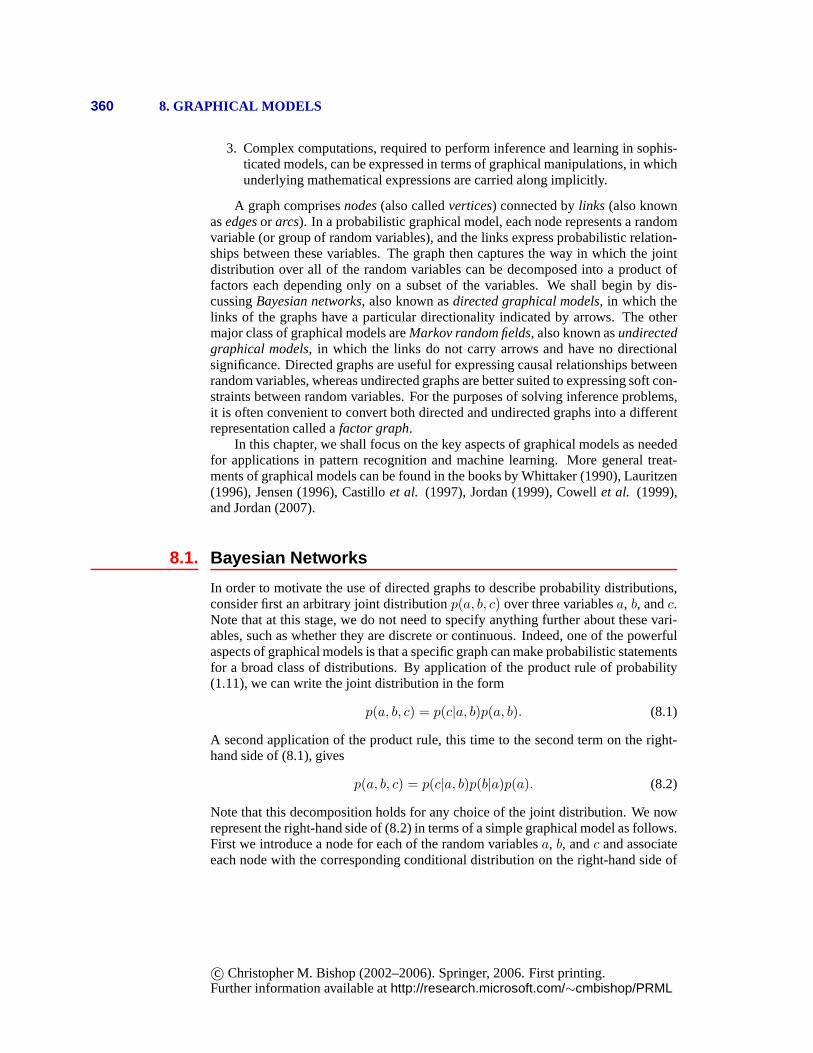
Figure 8.1 A directed graphical model representing the joint probabil-ity distribution over three variables a, b, and c, correspond-ing to the decomposition on the right-hand side of (8.2).
a
b
c
(8.2). Then, for each conditional distribution we add directed links (arrows) to thegraph from the nodes corresponding to the variables on whichthe distribution isconditioned. Thus for the factorp(c|a, b), there will be links from nodesa andb tonodec, whereas for the factorp(a) there will be no incoming links. The result isthe graph shown in Figure 8.1. If there is a link going from a nodea to a nodeb,then we say that nodea is theparentof nodeb, and we say that nodeb is thechildof nodea. Note that we shall not make any formal distinction between anode andthe variable to which it corresponds but will simply use the same symbol to refer toboth.
An interesting point to note about (8.2) is that the left-hand side is symmetricalwith respect to the three variablesa, b, andc, whereas the right-hand side is not.Indeed, in making the decomposition in (8.2), we have implicitly chosen a particularordering, namelya, b, c, and had we chosen a different ordering we would haveobtained a different decomposition and hence a different graphical representation.We shall return to this point later.
For the moment let us extend the example of Figure 8.1 by considering the jointdistribution overK variables given byp(x1, . . . , xK). By repeated application ofthe product rule of probability, this joint distribution can be written as a product ofconditional distributions, one for each of the variables
p(x1, . . . , xK) = p(xK |x1, . . . , xK−1) . . . p(x2|x1)p(x1). (8.3)
For a given choice ofK, we can again represent this as a directed graph havingKnodes, one for each conditional distribution on the right-hand side of (8.3), with eachnode having incoming links from all lower numbered nodes. Wesay that this graphis fully connectedbecause there is a link between every pair of nodes.
So far, we have worked with completely general joint distributions, so that thedecompositions, and their representations as fully connected graphs, will be applica-ble to any choice of distribution. As we shall see shortly, itis theabsenceof linksin the graph that conveys interesting information about theproperties of the class ofdistributions that the graph represents. Consider the graph shown in Figure 8.2.This is not a fully connected graph because, for instance, there is no link fromx1 tox2 or fromx3 to x7.
We shall now go from this graph to the corresponding representation of the jointprobability distribution written in terms of the product ofa set of conditional dis-tributions, one for each node in the graph. Each such conditional distribution willbe conditioned only on the parents of the corresponding nodein the graph. For in-stance,x5 will be conditioned onx1 andx3. The joint distribution of all7 variables
c© Christopher M. Bishop (2002–2006). Springer, 2006. First printing.Further information available athttp://research.microsoft.com/∼cmbishop/PRML
362 8. GRAPHICAL MODELS
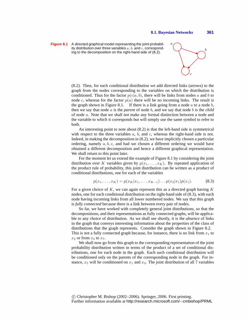
Figure 8.2 Example of a directed acyclic graph describing the jointdistribution over variables x1, . . . , x7. The correspondingdecomposition of the joint distribution is given by (8.4).
x1
x2 x3
x4 x5
x6 x7
is therefore given by
p(x1)p(x2)p(x3)p(x4|x1, x2, x3)p(x5|x1, x3)p(x6|x4)p(x7|x4, x5). (8.4)
The reader should take a moment to study carefully the correspondence between(8.4) and Figure 8.2.
We can now state in general terms the relationship between a given directedgraph and the corresponding distribution over the variables. The joint distributiondefined by a graph is given by the product, over all of the nodesof the graph, ofa conditional distribution for each node conditioned on thevariables correspondingto the parents of that node in the graph. Thus, for a graph withK nodes, the jointdistribution is given by
p(x) =
K∏
k=1
p(xk|pak) (8.5)
wherepak denotes the set of parents ofxk, andx = {x1, . . . , xK}. This keyequation expresses thefactorizationproperties of the joint distribution for a directedgraphical model. Although we have considered each node to correspond to a singlevariable, we can equally well associate sets of variables and vector-valued variableswith the nodes of a graph. It is easy to show that the representation on the right-hand side of (8.5) is always correctly normalized provided the individual conditionaldistributions are normalized.Exercise 8.1
The directed graphs that we are considering are subject to animportant restric-tion namely that there must be nodirected cycles, in other words there are no closedpaths within the graph such that we can move from node to node along links follow-ing the direction of the arrows and end up back at the startingnode. Such graphs arealso calleddirected acyclic graphs, or DAGs. This is equivalent to the statement thatExercise 8.2there exists an ordering of the nodes such that there are no links that go from anynode to any lower numbered node.
8.1.1 Example: Polynomial regressionAs an illustration of the use of directed graphs to describe probability distrib-
utions, we consider the Bayesian polynomial regression model introduced in Sec-
c© Christopher M. Bishop (2002–2006). Springer, 2006. First printing.Further information available athttp://research.microsoft.com/∼cmbishop/PRML
8.1. Bayesian Networks 363
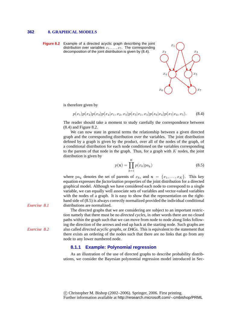
Figure 8.3 Directed graphical model representing the jointdistribution (8.6) corresponding to the Bayesianpolynomial regression model introduced in Sec-tion 1.2.6.
w
t1 tN
tion 1.2.6. The random variables in this model are the vectorof polynomial coeffi-cientsw and the observed datat = (t1, . . . , tN )T. In addition, this model containsthe input datax = (x1, . . . , xN )T, the noise varianceσ2, and the hyperparameterαrepresenting the precision of the Gaussian prior overw, all of which are parametersof the model rather than random variables. Focussing just onthe random variablesfor the moment, we see that the joint distribution is given bythe product of the priorp(w) andN conditional distributionsp(tn|w) for n = 1, . . . , N so that
p(t,w) = p(w)
N∏
n=1
p(tn|w). (8.6)
This joint distribution can be represented by a graphical model shown in Figure 8.3.
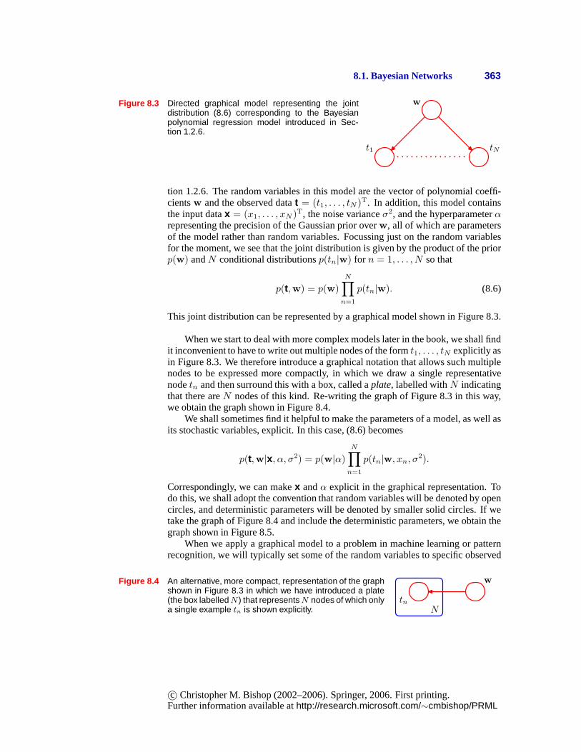
When we start to deal with more complex models later in the book, we shall findit inconvenient to have to write out multiple nodes of the form t1, . . . , tN explicitly asin Figure 8.3. We therefore introduce a graphical notation that allows such multiplenodes to be expressed more compactly, in which we draw a single representativenodetn and then surround this with a box, called aplate, labelled withN indicatingthat there areN nodes of this kind. Re-writing the graph of Figure 8.3 in thisway,we obtain the graph shown in Figure 8.4.
We shall sometimes find it helpful to make the parameters of a model, as well asits stochastic variables, explicit. In this case, (8.6) becomes
p(t,w|x, α, σ2) = p(w|α)
N∏
n=1
p(tn|w, xn, σ2).
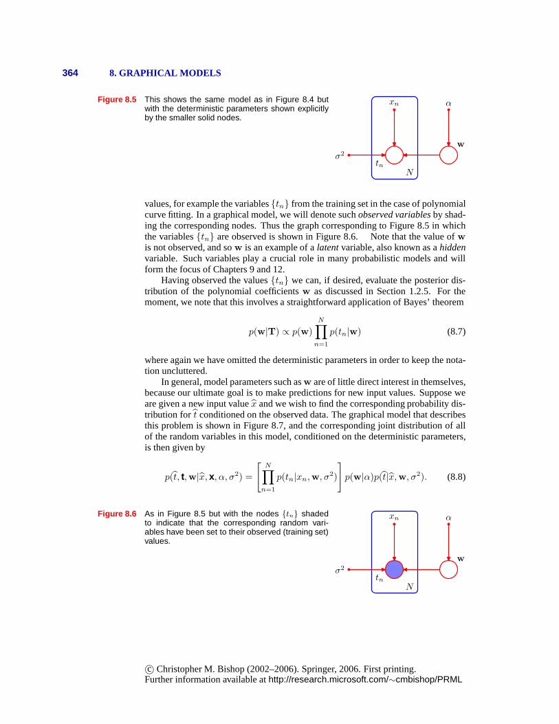
Correspondingly, we can makex andα explicit in the graphical representation. Todo this, we shall adopt the convention that random variableswill be denoted by opencircles, and deterministic parameters will be denoted by smaller solid circles. If wetake the graph of Figure 8.4 and include the deterministic parameters, we obtain thegraph shown in Figure 8.5.
When we apply a graphical model to a problem in machine learning or patternrecognition, we will typically set some of the random variables to specific observed
Figure 8.4 An alternative, more compact, representation of the graphshown in Figure 8.3 in which we have introduced a plate(the box labelledN ) that representsN nodes of which onlya single example tn is shown explicitly.
tnN
w
c© Christopher M. Bishop (2002–2006). Springer, 2006. First printing.Further information available athttp://research.microsoft.com/∼cmbishop/PRML
364 8. GRAPHICAL MODELS
Figure 8.5 This shows the same model as in Figure 8.4 butwith the deterministic parameters shown explicitlyby the smaller solid nodes.
tn
xn
N
w
α
σ2
values, for example the variables{tn} from the training set in the case of polynomialcurve fitting. In a graphical model, we will denote suchobserved variablesby shad-ing the corresponding nodes. Thus the graph corresponding to Figure 8.5 in whichthe variables{tn} are observed is shown in Figure 8.6. Note that the value ofw
is not observed, and sow is an example of alatentvariable, also known as ahiddenvariable. Such variables play a crucial role in many probabilistic models and willform the focus of Chapters 9 and 12.
Having observed the values{tn} we can, if desired, evaluate the posterior dis-tribution of the polynomial coefficientsw as discussed in Section 1.2.5. For themoment, we note that this involves a straightforward application of Bayes’ theorem
p(w|T) ∝ p(w)
N∏
n=1
p(tn|w) (8.7)
where again we have omitted the deterministic parameters inorder to keep the nota-tion uncluttered.
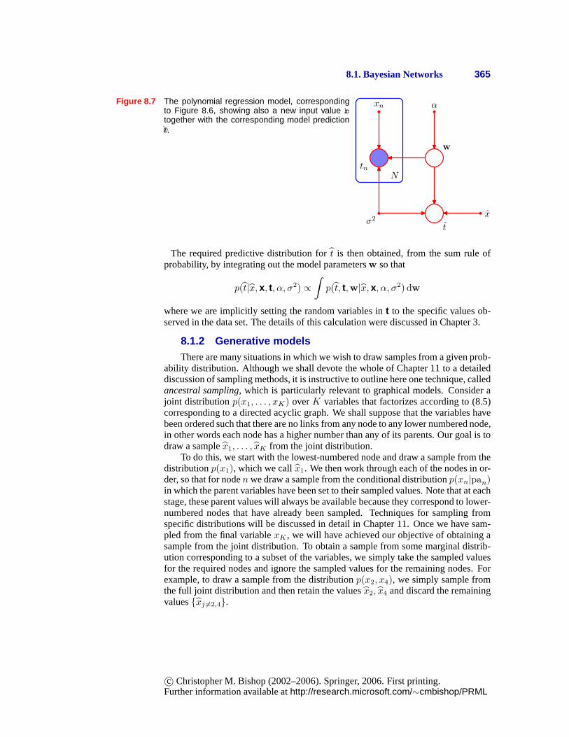
In general, model parameters such asw are of little direct interest in themselves,because our ultimate goal is to make predictions for new input values. Suppose weare given a new input valuex and we wish to find the corresponding probability dis-tribution for t conditioned on the observed data. The graphical model that describesthis problem is shown in Figure 8.7, and the corresponding joint distribution of allof the random variables in this model, conditioned on the deterministic parameters,is then given by
p(t, t,w|x, x, α, σ2) =
[N∏
n=1
p(tn|xn,w, σ2)
]p(w|α)p(t|x,w, σ2). (8.8)
Figure 8.6 As in Figure 8.5 but with the nodes {tn} shadedto indicate that the corresponding random vari-ables have been set to their observed (training set)values.
tn
xn
N
w
α
σ2
c© Christopher M. Bishop (2002–2006). Springer, 2006. First printing.Further information available athttp://research.microsoft.com/∼cmbishop/PRML
8.1. Bayesian Networks 365
Figure 8.7 The polynomial regression model, correspondingto Figure 8.6, showing also a new input value bxtogether with the corresponding model predictionbt.
tn
xn
N
w
α
tσ2
x
The required predictive distribution fort is then obtained, from the sum rule ofprobability, by integrating out the model parametersw so that
p(t|x, x, t, α, σ2) ∝∫p(t, t,w|x, x, α, σ2) dw
where we are implicitly setting the random variables int to the specific values ob-served in the data set. The details of this calculation were discussed in Chapter 3.
8.1.2 Generative modelsThere are many situations in which we wish to draw samples from a given prob-
ability distribution. Although we shall devote the whole ofChapter 11 to a detaileddiscussion of sampling methods, it is instructive to outline here one technique, calledancestral sampling, which is particularly relevant to graphical models. Consider ajoint distributionp(x1, . . . , xK) overK variables that factorizes according to (8.5)corresponding to a directed acyclic graph. We shall supposethat the variables havebeen ordered such that there are no links from any node to any lower numbered node,in other words each node has a higher number than any of its parents. Our goal is todraw a samplex1, . . . , xK from the joint distribution.
To do this, we start with the lowest-numbered node and draw a sample from thedistributionp(x1), which we callx1. We then work through each of the nodes in or-der, so that for nodenwe draw a sample from the conditional distributionp(xn|pan)in which the parent variables have been set to their sampled values. Note that at eachstage, these parent values will always be available becausethey correspond to lower-numbered nodes that have already been sampled. Techniques for sampling fromspecific distributions will be discussed in detail in Chapter 11. Once we have sam-pled from the final variablexK , we will have achieved our objective of obtaining asample from the joint distribution. To obtain a sample from some marginal distrib-ution corresponding to a subset of the variables, we simply take the sampled valuesfor the required nodes and ignore the sampled values for the remaining nodes. Forexample, to draw a sample from the distributionp(x2, x4), we simply sample fromthe full joint distribution and then retain the valuesx2, x4 and discard the remainingvalues{xj 6=2,4}.
c© Christopher M. Bishop (2002–2006). Springer, 2006. First printing.Further information available athttp://research.microsoft.com/∼cmbishop/PRML
366 8. GRAPHICAL MODELS
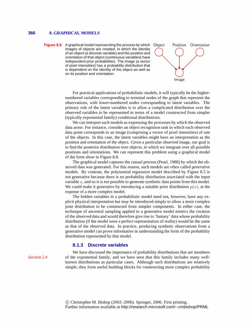
Figure 8.8 A graphical model representing the process by whichimages of objects are created, in which the identityof an object (a discrete variable) and the position andorientation of that object (continuous variables) haveindependent prior probabilities. The image (a vectorof pixel intensities) has a probability distribution thatis dependent on the identity of the object as well ason its position and orientation.
Image
Object OrientationPosition
For practical applications of probabilistic models, it will typically be the higher-numbered variables corresponding to terminal nodes of the graph that represent theobservations, with lower-numbered nodes corresponding tolatent variables. Theprimary role of the latent variables is to allow a complicated distribution over theobserved variables to be represented in terms of a model constructed from simpler(typically exponential family) conditional distributions.
We can interpret such models as expressing the processes by which the observeddata arose. For instance, consider an object recognition task in which each observeddata point corresponds to an image (comprising a vector of pixel intensities) of oneof the objects. In this case, the latent variables might havean interpretation as theposition and orientation of the object. Given a particular observed image, our goal isto find the posterior distribution over objects, in which we integrate over all possiblepositions and orientations. We can represent this problem using a graphical modelof the form show in Figure 8.8.
The graphical model captures thecausalprocess (Pearl, 1988) by which the ob-served data was generated. For this reason, such models are often calledgenerativemodels. By contrast, the polynomial regression model described by Figure 8.5 isnot generative because there is no probability distribution associated with the inputvariablex, and so it is not possible to generate synthetic data points from this model.We could make it generative by introducing a suitable prior distributionp(x), at theexpense of a more complex model.
The hidden variables in a probabilistic model need not, however, have any ex-plicit physical interpretation but may be introduced simply to allow a more complexjoint distribution to be constructed from simpler components. In either case, thetechnique of ancestral sampling applied to a generative model mimics the creationof the observed data and would therefore give rise to ‘fantasy’ data whose probabilitydistribution (if the model were a perfect representation ofreality) would be the sameas that of the observed data. In practice, producing synthetic observations from agenerative model can prove informative in understanding the form of the probabilitydistribution represented by that model.
8.1.3 Discrete variablesWe have discussed the importance of probability distributions that are members
of the exponential family, and we have seen that this family includes many well-Section 2.4known distributions as particular cases. Although such distributions are relativelysimple, they form useful building blocks for constructing more complex probability
c© Christopher M. Bishop (2002–2006). Springer, 2006. First printing.Further information available athttp://research.microsoft.com/∼cmbishop/PRML
8.1. Bayesian Networks 367
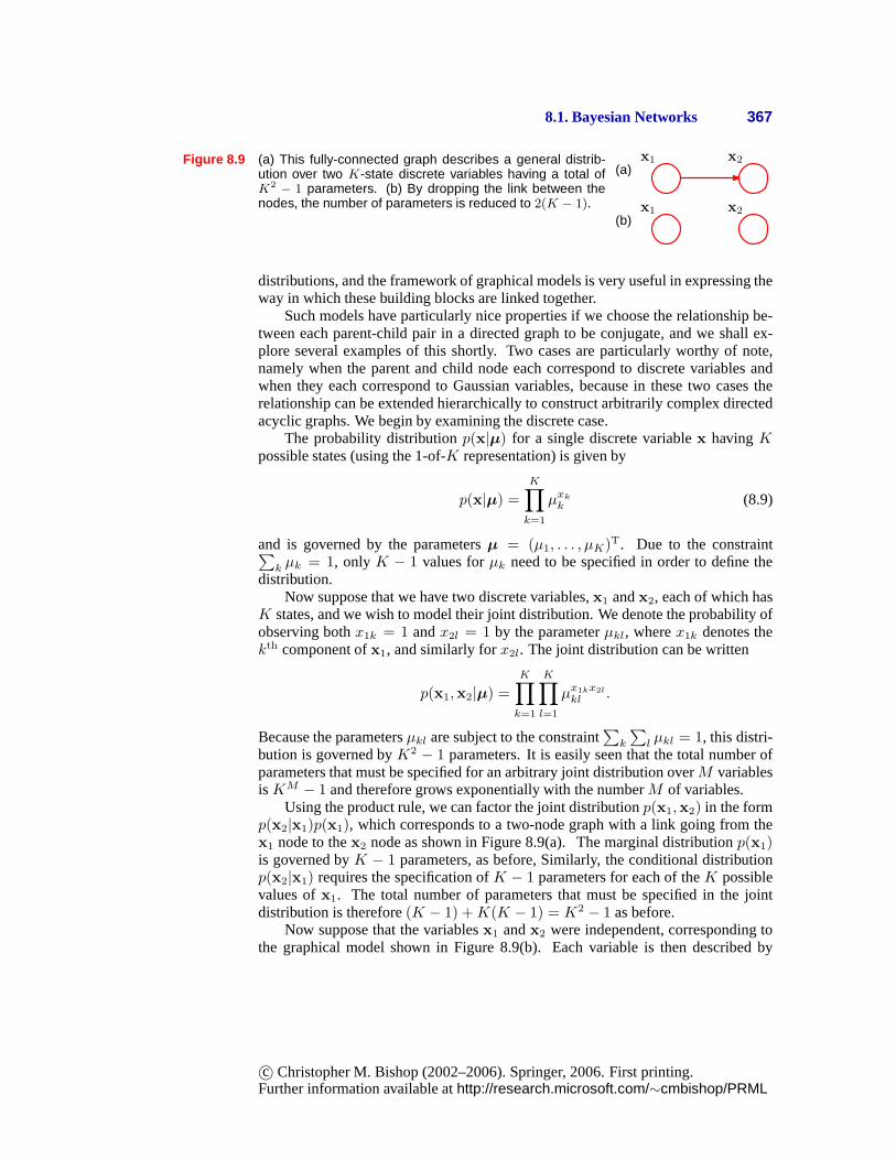
Figure 8.9 (a) This fully-connected graph describes a general distrib-ution over two K-state discrete variables having a total ofK2 − 1 parameters. (b) By dropping the link between thenodes, the number of parameters is reduced to 2(K − 1).
(a)x1 x2
(b)x1 x2
distributions, and the framework of graphical models is very useful in expressing theway in which these building blocks are linked together.
Such models have particularly nice properties if we choose the relationship be-tween each parent-child pair in a directed graph to be conjugate, and we shall ex-plore several examples of this shortly. Two cases are particularly worthy of note,namely when the parent and child node each correspond to discrete variables andwhen they each correspond to Gaussian variables, because inthese two cases therelationship can be extended hierarchically to construct arbitrarily complex directedacyclic graphs. We begin by examining the discrete case.
The probability distributionp(x|µ) for a single discrete variablex havingKpossible states (using the 1-of-K representation) is given by
p(x|µ) =
K∏
k=1
µxk
k (8.9)
and is governed by the parametersµ = (µ1, . . . , µK)T. Due to the constraint∑k µk = 1, onlyK − 1 values forµk need to be specified in order to define the
distribution.Now suppose that we have two discrete variables,x1 andx2, each of which has
K states, and we wish to model their joint distribution. We denote the probability ofobserving bothx1k = 1 andx2l = 1 by the parameterµkl, wherex1k denotes thekth component ofx1, and similarly forx2l. The joint distribution can be written
p(x1,x2|µ) =
K∏
k=1
K∏
l=1
µx1kx2l
kl .
Because the parametersµkl are subject to the constraint∑
k
∑l µkl = 1, this distri-
bution is governed byK2 − 1 parameters. It is easily seen that the total number ofparameters that must be specified for an arbitrary joint distribution overM variablesisKM − 1 and therefore grows exponentially with the numberM of variables.
Using the product rule, we can factor the joint distributionp(x1,x2) in the formp(x2|x1)p(x1), which corresponds to a two-node graph with a link going fromthex1 node to thex2 node as shown in Figure 8.9(a). The marginal distributionp(x1)is governed byK − 1 parameters, as before, Similarly, the conditional distributionp(x2|x1) requires the specification ofK − 1 parameters for each of theK possiblevalues ofx1. The total number of parameters that must be specified in the jointdistribution is therefore(K − 1) +K(K − 1) = K2 − 1 as before.
Now suppose that the variablesx1 andx2 were independent, corresponding tothe graphical model shown in Figure 8.9(b). Each variable isthen described by
c© Christopher M. Bishop (2002–2006). Springer, 2006. First printing.Further information available athttp://research.microsoft.com/∼cmbishop/PRML
368 8. GRAPHICAL MODELS
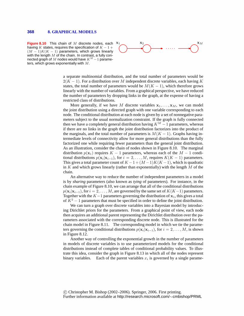
Figure 8.10 This chain of M discrete nodes, eachhaving K states, requires the specification of K − 1 +(M − 1)K(K − 1) parameters, which grows linearlywith the length M of the chain. In contrast, a fully con-nected graph of M nodes would haveKM −1 parame-ters, which grows exponentially with M .
x1 x2 xM
a separate multinomial distribution, and the total number of parameters would be2(K − 1). For a distribution overM independent discrete variables, each havingKstates, the total number of parameters would beM (K − 1), which therefore growslinearly with the number of variables. From a graphical perspective, we have reducedthe number of parameters by dropping links in the graph, at the expense of having arestricted class of distributions.
More generally, if we haveM discrete variablesx1, . . . ,xM , we can modelthe joint distribution using a directed graph with one variable corresponding to eachnode. The conditional distribution at each node is given by aset of nonnegative para-meters subject to the usual normalization constraint. If the graph is fully connectedthen we have a completely general distribution havingKM − 1 parameters, whereasif there are no links in the graph the joint distribution factorizes into the product ofthe marginals, and the total number of parameters isM (K − 1). Graphs having in-termediate levels of connectivity allow for more general distributions than the fullyfactorized one while requiring fewer parameters than the general joint distribution.As an illustration, consider the chain of nodes shown in Figure 8.10. The marginaldistributionp(x1) requiresK − 1 parameters, whereas each of theM − 1 condi-tional distributionsp(xi|xi−1), for i = 2, . . . ,M , requiresK(K − 1) parameters.This gives a total parameter count ofK−1+(M−1)K(K−1), which is quadraticin K and which grows linearly (rather than exponentially) with the lengthM of thechain.
An alternative way to reduce the number of independent parameters in a modelis by sharingparameters (also known astying of parameters). For instance, in thechain example of Figure 8.10, we can arrange that all of the conditional distributionsp(xi|xi−1), for i = 2, . . . ,M , are governed by the same set ofK(K−1) parameters.Together with theK−1 parameters governing the distribution ofx1, this gives a totalof K2 − 1 parameters that must be specified in order to define the joint distribution.
We can turn a graph over discrete variables into a Bayesian model by introduc-ing Dirichlet priors for the parameters. From a graphical point of view, each nodethen acquires an additional parent representing the Dirichlet distribution over the pa-rameters associated with the corresponding discrete node.This is illustrated for thechain model in Figure 8.11. The corresponding model in whichwe tie the parame-ters governing the conditional distributionsp(xi|xi−1), for i = 2, . . . ,M , is shownin Figure 8.12.
Another way of controlling the exponential growth in the number of parametersin models of discrete variables is to use parameterized models for the conditionaldistributions instead of complete tables of conditional probability values. To illus-trate this idea, consider the graph in Figure 8.13 in which all of the nodes representbinary variables. Each of the parent variablesxi is governed by a single parame-
c© Christopher M. Bishop (2002–2006). Springer, 2006. First printing.Further information available athttp://research.microsoft.com/∼cmbishop/PRML
8.1. Bayesian Networks 369
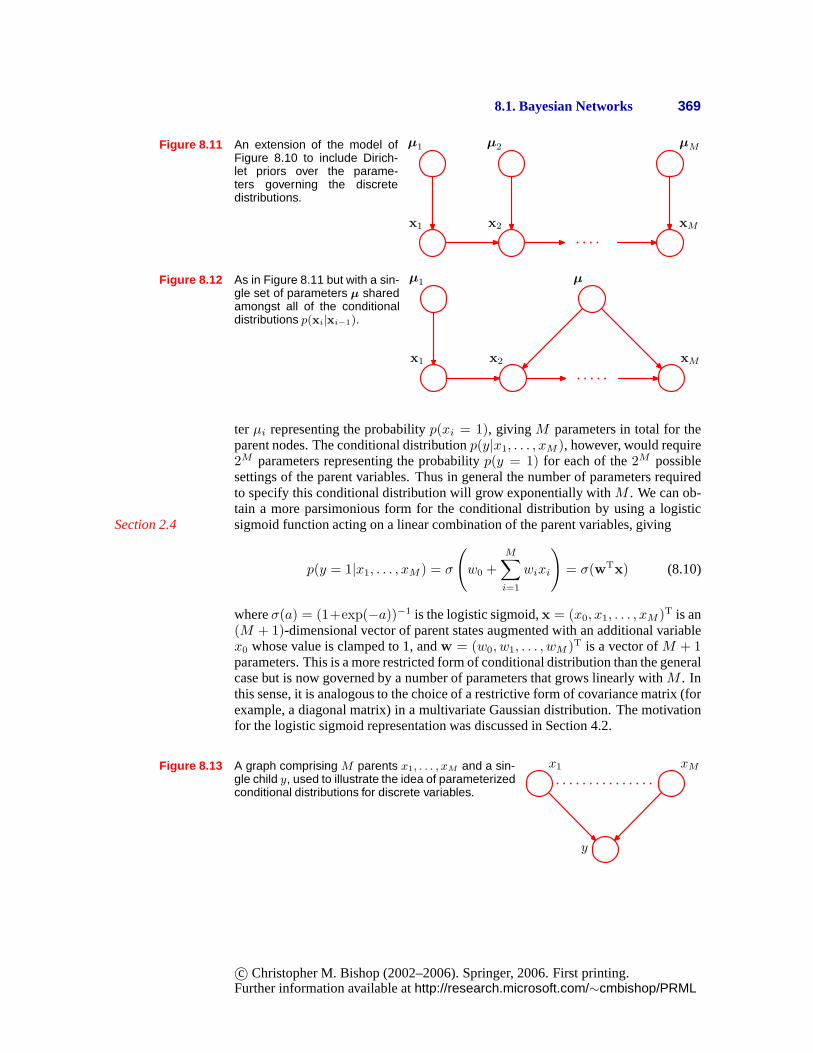
Figure 8.11 An extension of the model ofFigure 8.10 to include Dirich-let priors over the parame-ters governing the discretedistributions.
x1 x2 xM
µ1 µ2 µM
Figure 8.12 As in Figure 8.11 but with a sin-gle set of parameters µ sharedamongst all of the conditionaldistributions p(xi|xi−1).
x1 x2 xM
µ1 µ
ter µi representing the probabilityp(xi = 1), givingM parameters in total for theparent nodes. The conditional distributionp(y|x1, . . . , xM ), however, would require2M parameters representing the probabilityp(y = 1) for each of the2M possiblesettings of the parent variables. Thus in general the numberof parameters requiredto specify this conditional distribution will grow exponentially with M . We can ob-tain a more parsimonious form for the conditional distribution by using a logisticsigmoid function acting on a linear combination of the parent variables, givingSection 2.4
p(y = 1|x1, . . . , xM ) = σ
(w0 +
M∑
i=1
wixi
)= σ(wTx) (8.10)
whereσ(a) = (1+exp(−a))−1 is the logistic sigmoid,x = (x0, x1, . . . , xM )T is an(M + 1)-dimensional vector of parent states augmented with an additional variablex0 whose value is clamped to 1, andw = (w0, w1, . . . , wM )T is a vector ofM + 1parameters. This is a more restricted form of conditional distribution than the generalcase but is now governed by a number of parameters that grows linearly withM . Inthis sense, it is analogous to the choice of a restrictive form of covariance matrix (forexample, a diagonal matrix) in a multivariate Gaussian distribution. The motivationfor the logistic sigmoid representation was discussed in Section 4.2.
Figure 8.13 A graph comprising M parents x1, . . . , xM and a sin-gle child y, used to illustrate the idea of parameterizedconditional distributions for discrete variables.
y
x1 xM
c© Christopher M. Bishop (2002–2006). Springer, 2006. First printing.Further information available athttp://research.microsoft.com/∼cmbishop/PRML
370 8. GRAPHICAL MODELS
8.1.4 Linear-Gaussian modelsIn the previous section, we saw how to construct joint probability distributions
over a set of discrete variables by expressing the variablesas nodes in a directedacyclic graph. Here we show how a multivariate Gaussian can be expressed as adirected graph corresponding to a linear-Gaussian model over the component vari-ables. This allows us to impose interesting structure on thedistribution, with thegeneral Gaussian and the diagonal covariance Gaussian representing opposite ex-tremes. Several widely used techniques are examples of linear-Gaussian models,such as probabilistic principal component analysis, factor analysis, and linear dy-namical systems (Roweis and Ghahramani, 1999). We shall make extensive use ofthe results of this section in later chapters when we consider some of these techniquesin detail.
Consider an arbitrary directed acyclic graph overD variables in which nodeirepresents a single continuous random variablexi having a Gaussian distribution.The mean of this distribution is taken to be a linear combination of the states of itsparent nodespai of nodei
p(xi|pai) = N
xi
∣∣∣∣∣∣
∑
j∈pai
wijxj + bi, vi
(8.11)
wherewij andbi are parameters governing the mean, andvi is the variance of theconditional distribution forxi. The log of the joint distribution is then the log of theproduct of these conditionals over all nodes in the graph andhence takes the form
ln p(x) =
D∑
i=1
ln p(xi|pai) (8.12)
= −D∑
i=1
1
2vi
xi −
∑
j∈pai
wijxj − bi
2
+ const (8.13)
wherex = (x1, . . . , xD)T and ‘const’ denotes terms independent ofx. We see thatthis is a quadratic function of the components ofx, and hence the joint distributionp(x) is a multivariate Gaussian.
We can determine the mean and covariance of the joint distribution recursivelyas follows. Each variablexi has (conditional on the states of its parents) a Gaussiandistribution of the form (8.11) and so
xi =∑
j∈pai
wijxj + bi +√viεi (8.14)
whereεi is a zero mean, unit variance Gaussian random variable satisfying E[εi] = 0andE[εiεj ] = Iij, whereIij is thei, j element of the identity matrix. Taking theexpectation of (8.14), we have
E[xi] =∑
j∈pai
wijE[xj ] + bi. (8.15)
c© Christopher M. Bishop (2002–2006). Springer, 2006. First printing.Further information available athttp://research.microsoft.com/∼cmbishop/PRML
8.1. Bayesian Networks 371
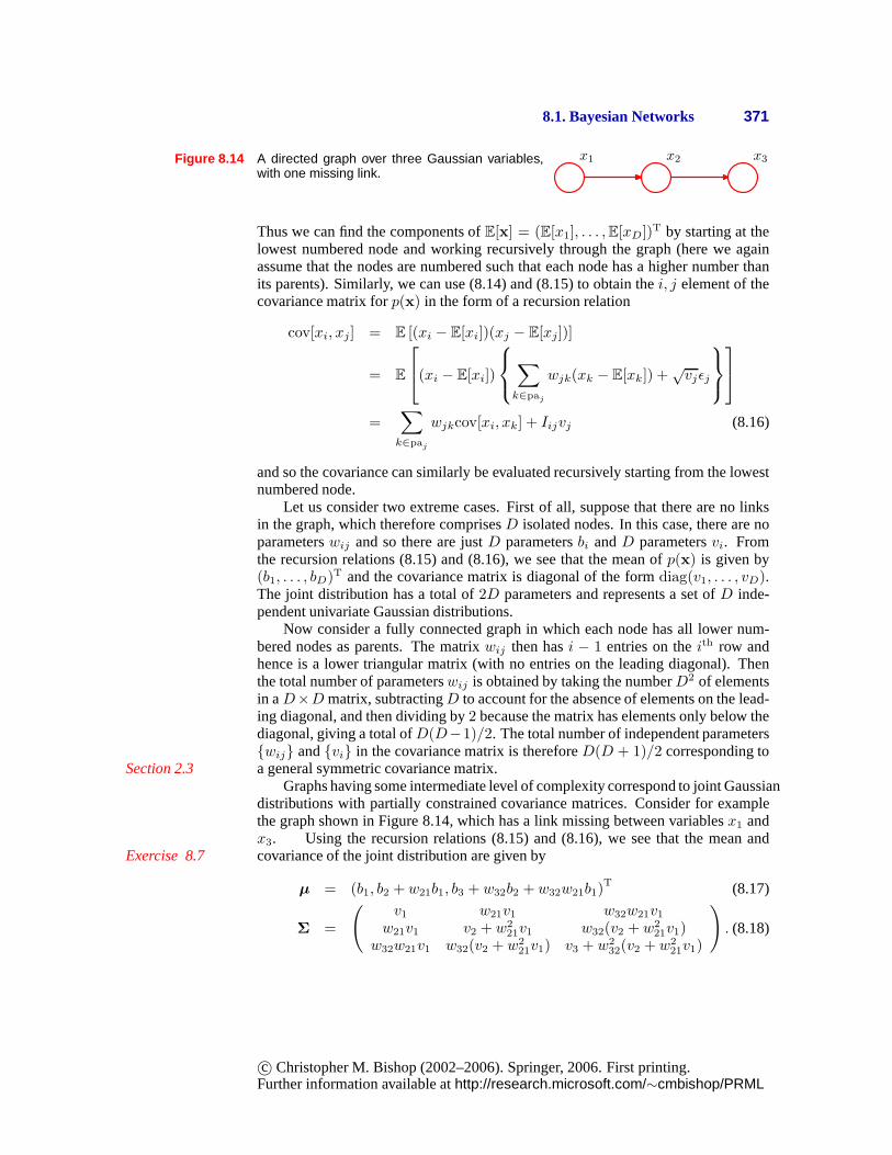
Figure 8.14 A directed graph over three Gaussian variables,with one missing link.
x1 x2 x3
Thus we can find the components ofE[x] = (E[x1], . . . ,E[xD])T by starting at thelowest numbered node and working recursively through the graph (here we againassume that the nodes are numbered such that each node has a higher number thanits parents). Similarly, we can use (8.14) and (8.15) to obtain thei, j element of thecovariance matrix forp(x) in the form of a recursion relation
cov[xi, xj] = E [(xi − E[xi])(xj − E[xj])]
= E
(xi − E[xi])
∑
k∈paj
wjk(xk − E[xk]) +√vjεj
=∑
k∈paj
wjkcov[xi, xk] + Iijvj (8.16)
and so the covariance can similarly be evaluated recursively starting from the lowestnumbered node.
Let us consider two extreme cases. First of all, suppose thatthere are no linksin the graph, which therefore comprisesD isolated nodes. In this case, there are noparameterswij and so there are justD parametersbi andD parametersvi. Fromthe recursion relations (8.15) and (8.16), we see that the mean ofp(x) is given by(b1, . . . , bD)T and the covariance matrix is diagonal of the formdiag(v1, . . . , vD).The joint distribution has a total of2D parameters and represents a set ofD inde-pendent univariate Gaussian distributions.
Now consider a fully connected graph in which each node has all lower num-bered nodes as parents. The matrixwij then hasi − 1 entries on theith row andhence is a lower triangular matrix (with no entries on the leading diagonal). Thenthe total number of parameterswij is obtained by taking the numberD2 of elementsin aD×D matrix, subtractingD to account for the absence of elements on the lead-ing diagonal, and then dividing by2 because the matrix has elements only below thediagonal, giving a total ofD(D−1)/2. The total number of independent parameters{wij} and{vi} in the covariance matrix is thereforeD(D + 1)/2 corresponding toa general symmetric covariance matrix.Section 2.3
Graphs having some intermediate level of complexity correspond to joint Gaussiandistributions with partially constrained covariance matrices. Consider for examplethe graph shown in Figure 8.14, which has a link missing between variablesx1 andx3. Using the recursion relations (8.15) and (8.16), we see that the mean andcovariance of the joint distribution are given byExercise 8.7
µ = (b1, b2 + w21b1, b3 + w32b2 + w32w21b1)T (8.17)
Σ =
(v1 w21v1 w32w21v1
w21v1 v2 + w221v1 w32(v2 + w2
21v1)w32w21v1 w32(v2 + w2
21v1) v3 + w232(v2 + w2
21v1)
). (8.18)
c© Christopher M. Bishop (2002–2006). Springer, 2006. First printing.Further information available athttp://research.microsoft.com/∼cmbishop/PRML
372 8. GRAPHICAL MODELS
We can readily extend the linear-Gaussian graphical model to the case in whichthe nodes of the graph represent multivariate Gaussian variables. In this case, we canwrite the conditional distribution for nodei in the form
p(xi|pai) = N
xi
∣∣∣∣∣∣
∑
j∈pai
Wijxj + bi,Σi
(8.19)
where nowWij is a matrix (which is nonsquare ifxi andxj have different dimen-sionalities). Again it is easy to verify that the joint distribution over all variables isGaussian.
Note that we have already encountered a specific example of the linear-Gaussianrelationship when we saw that the conjugate prior for the mean µ of a GaussianSection 2.3.6variablex is itself a Gaussian distribution overµ. The joint distribution overx andµ is therefore Gaussian. This corresponds to a simple two-node graph in whichthe node representingµ is the parent of the node representingx. The mean of thedistribution overµ is a parameter controlling a prior, and so it can be viewed as ahyperparameter. Because the value of this hyperparameter may itself be unknown,we can again treat it from a Bayesian perspective by introducing a prior over thehyperparameter, sometimes called ahyperprior, which is again given by a Gaussiandistribution. This type of construction can be extended in principle to any level and isan illustration of ahierarchical Bayesian model, of which we shall encounter furtherexamples in later chapters.
8.2. Conditional Independence
An important concept for probability distributions over multiple variables is that ofconditional independence(Dawid, 1980). Consider three variablesa, b, andc, andsuppose that the conditional distribution ofa, givenb andc, is such that it does notdepend on the value ofb, so that
p(a|b, c) = p(a|c). (8.20)
We say thata is conditionally independent ofb givenc. This can be expressed in aslightly different way if we consider the joint distribution of a andb conditioned onc, which we can write in the form
p(a, b|c) = p(a|b, c)p(b|c)= p(a|c)p(b|c). (8.21)
where we have used the product rule of probability together with (8.20). Thus wesee that, conditioned onc, the joint distribution ofa andb factorizes into the prod-uct of the marginal distribution ofa and the marginal distribution ofb (again bothconditioned onc). This says that the variablesa andb are statistically independent,givenc. Note that our definition of conditional independence will require that (8.20),
c© Christopher M. Bishop (2002–2006). Springer, 2006. First printing.Further information available athttp://research.microsoft.com/∼cmbishop/PRML
8.2. Conditional Independence 373
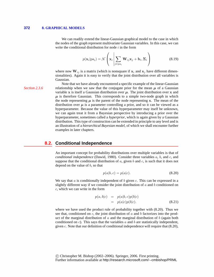
Figure 8.15 The first of three examples of graphs over three variablesa, b, and c used to discuss conditional independenceproperties of directed graphical models.
c
a b
or equivalently (8.21), must hold for every possible value of c, and not just for somevalues. We shall sometimes use a shorthand notation for conditional independence(Dawid, 1979) in which
a ⊥⊥ b | c (8.22)
denotes thata is conditionally independent ofb givenc and is equivalent to (8.20).Conditional independence properties play an important role in using probabilis-
tic models for pattern recognition by simplifying both the structure of a model andthe computations needed to perform inference and learning under that model. Weshall see examples of this shortly.
If we are given an expression for the joint distribution overa set of variables interms of a product of conditional distributions (i.e., the mathematical representationunderlying a directed graph), then we could in principle test whether any poten-tial conditional independence property holds by repeated application of the sum andproduct rules of probability. In practice, such an approachwould be very time con-suming. An important and elegant feature of graphical models is that conditionalindependence properties of the joint distribution can be read directly from the graphwithout having to perform any analytical manipulations. The general frameworkfor achieving this is calledd-separation, where the ‘d’ stands for ‘directed’ (Pearl,1988). Here we shall motivate the concept of d-separation and give a general state-ment of the d-separation criterion. A formal proof can be found in Lauritzen (1996).
8.2.1 Three example graphsWe begin our discussion of the conditional independence properties of directed
graphs by considering three simple examples each involvinggraphs having just threenodes. Together, these will motivate and illustrate the keyconcepts of d-separation.The first of the three examples is shown in Figure 8.15, and thejoint distributioncorresponding to this graph is easily written down using thegeneral result (8.5) togive
p(a, b, c) = p(a|c)p(b|c)p(c). (8.23)
If none of the variables are observed, then we can investigate whethera andb areindependent by marginalizing both sides of (8.23) with respect toc to give
p(a, b) =∑
c
p(a|c)p(b|c)p(c). (8.24)
In general, this does not factorize into the productp(a)p(b), and so
a 6⊥⊥ b | ∅ (8.25)
c© Christopher M. Bishop (2002–2006). Springer, 2006. First printing.Further information available athttp://research.microsoft.com/∼cmbishop/PRML
374 8. GRAPHICAL MODELS
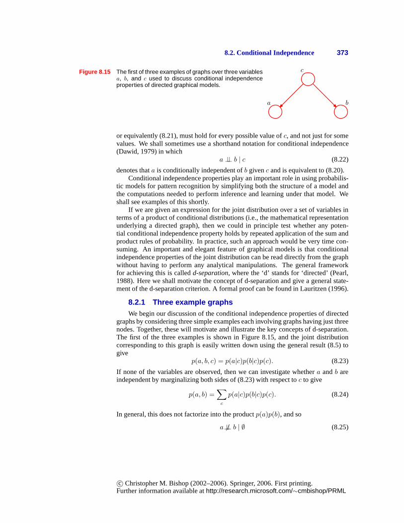
Figure 8.16 As in Figure 8.15 but where we have conditioned on thevalue of variable c.
c
a b
where∅ denotes the empty set, and the symbol6⊥⊥ means that the conditional inde-pendence property does not hold in general. Of course, it mayhold for a particulardistribution by virtue of the specific numerical values associated with the variousconditional probabilities, but it does not follow in general from the structure of thegraph.
Now suppose we condition on the variablec, as represented by the graph ofFigure 8.16. From (8.23), we can easily write down the conditional distribution ofa andb, givenc, in the form
p(a, b|c) =p(a, b, c)
p(c)
= p(a|c)p(b|c)
and so we obtain the conditional independence property
a ⊥⊥ b | c.
We can provide a simple graphical interpretation of this result by consideringthe path from nodea to nodeb via c. The nodec is said to betail-to-tail with re-spect to this path because the node is connected to the tails of the two arrows, andthe presence of such a path connecting nodesa andb causes these nodes to be de-pendent. However, when we condition on nodec, as in Figure 8.16, the conditionednode ‘blocks’ the path froma to b and causesa and b to become (conditionally)independent.
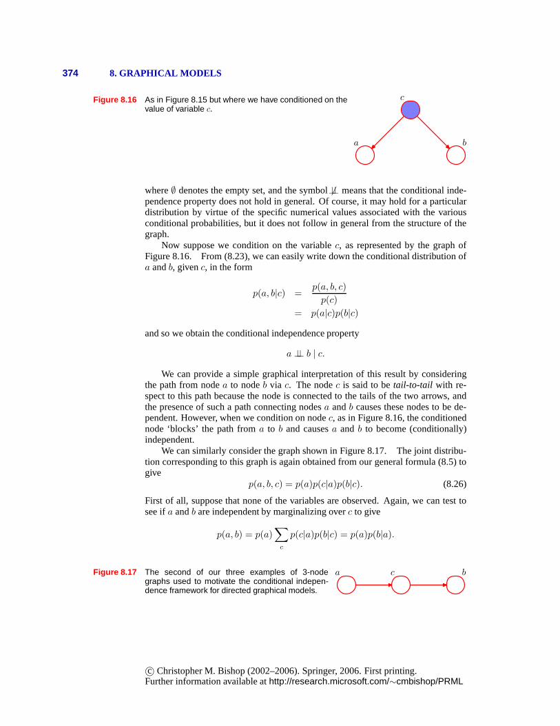
We can similarly consider the graph shown in Figure 8.17. Thejoint distribu-tion corresponding to this graph is again obtained from our general formula (8.5) togive
p(a, b, c) = p(a)p(c|a)p(b|c). (8.26)
First of all, suppose that none of the variables are observed. Again, we can test tosee ifa andb are independent by marginalizing overc to give
p(a, b) = p(a)∑
c
p(c|a)p(b|c) = p(a)p(b|a).
Figure 8.17 The second of our three examples of 3-nodegraphs used to motivate the conditional indepen-dence framework for directed graphical models.
a c b
c© Christopher M. Bishop (2002–2006). Springer, 2006. First printing.Further information available athttp://research.microsoft.com/∼cmbishop/PRML
8.2. Conditional Independence 375
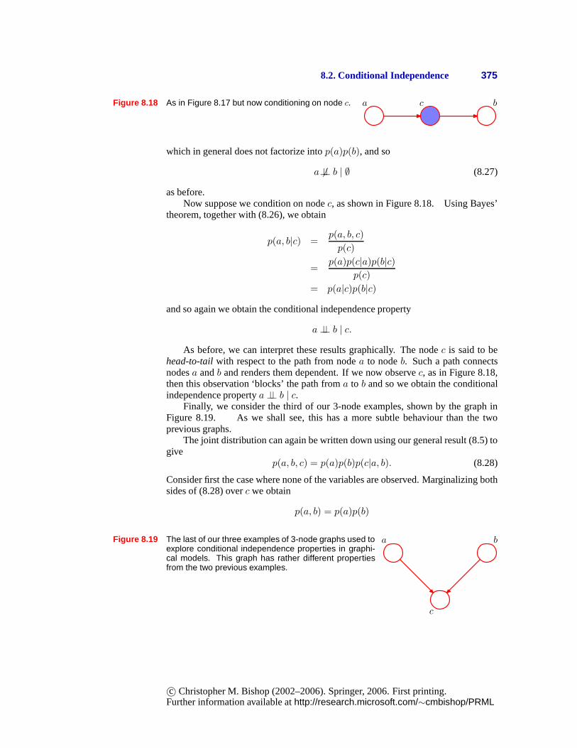
Figure 8.18 As in Figure 8.17 but now conditioning on node c. a c b
which in general does not factorize intop(a)p(b), and so
a 6⊥⊥ b | ∅ (8.27)
as before.Now suppose we condition on nodec, as shown in Figure 8.18. Using Bayes’
theorem, together with (8.26), we obtain
p(a, b|c) =p(a, b, c)
p(c)
=p(a)p(c|a)p(b|c)
p(c)
= p(a|c)p(b|c)
and so again we obtain the conditional independence property
a ⊥⊥ b | c.
As before, we can interpret these results graphically. The nodec is said to behead-to-tailwith respect to the path from nodea to nodeb. Such a path connectsnodesa andb and renders them dependent. If we now observec, as in Figure 8.18,then this observation ‘blocks’ the path froma to b and so we obtain the conditionalindependence propertya ⊥⊥ b | c.
Finally, we consider the third of our 3-node examples, shownby the graph inFigure 8.19. As we shall see, this has a more subtle behaviourthan the twoprevious graphs.
The joint distribution can again be written down using our general result (8.5) togive
p(a, b, c) = p(a)p(b)p(c|a, b). (8.28)
Consider first the case where none of the variables are observed. Marginalizing bothsides of (8.28) overc we obtain
p(a, b) = p(a)p(b)
Figure 8.19 The last of our three examples of 3-node graphs used toexplore conditional independence properties in graphi-cal models. This graph has rather different propertiesfrom the two previous examples.
c
a b
c© Christopher M. Bishop (2002–2006). Springer, 2006. First printing.Further information available athttp://research.microsoft.com/∼cmbishop/PRML
376 8. GRAPHICAL MODELS
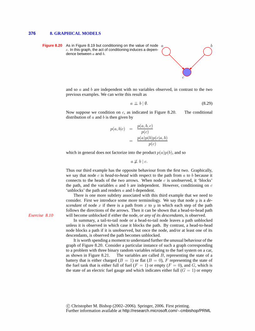
Figure 8.20 As in Figure 8.19 but conditioning on the value of nodec. In this graph, the act of conditioning induces a depen-dence between a and b.
c
a b
and soa andb are independent with no variables observed, in contrast to the twoprevious examples. We can write this result as
a ⊥⊥ b | ∅. (8.29)
Now suppose we condition onc, as indicated in Figure 8.20. The conditionaldistribution ofa andb is then given by
p(a, b|c) =p(a, b, c)
p(c)
=p(a)p(b)p(c|a, b)
p(c)
which in general does not factorize into the productp(a)p(b), and so
a 6⊥⊥ b | c.
Thus our third example has the opposite behaviour from the first two. Graphically,we say that nodec is head-to-headwith respect to the path froma to b because itconnects to the heads of the two arrows. When nodec is unobserved, it ‘blocks’the path, and the variablesa and b are independent. However, conditioning onc‘unblocks’ the path and rendersa andb dependent.
There is one more subtlety associated with this third example that we need toconsider. First we introduce some more terminology. We say that nodey is a de-scendantof nodex if there is a path fromx to y in which each step of the pathfollows the directions of the arrows. Then it can be shown that a head-to-head pathwill become unblocked if either the node,or any of its descendants, is observed.Exercise 8.10
In summary, a tail-to-tail node or a head-to-tail node leaves a path unblockedunless it is observed in which case it blocks the path. By contrast, a head-to-headnode blocks a path if it is unobserved, but once the node, and/or at least one of itsdescendants, is observed the path becomes unblocked.
It is worth spending a moment to understand further the unusual behaviour of thegraph of Figure 8.20. Consider a particular instance of sucha graph correspondingto a problem with three binary random variables relating to the fuel system on a car,as shown in Figure 8.21. The variables are calledB, representing the state of abattery that is either charged (B = 1) or flat (B = 0), F representing the state ofthe fuel tank that is either full of fuel (F = 1) or empty (F = 0), andG, which isthe state of an electric fuel gauge and which indicates either full (G = 1) or empty
c© Christopher M. Bishop (2002–2006). Springer, 2006. First printing.Further information available athttp://research.microsoft.com/∼cmbishop/PRML
8.2. Conditional Independence 377
G
B F
G
B F
G
B F
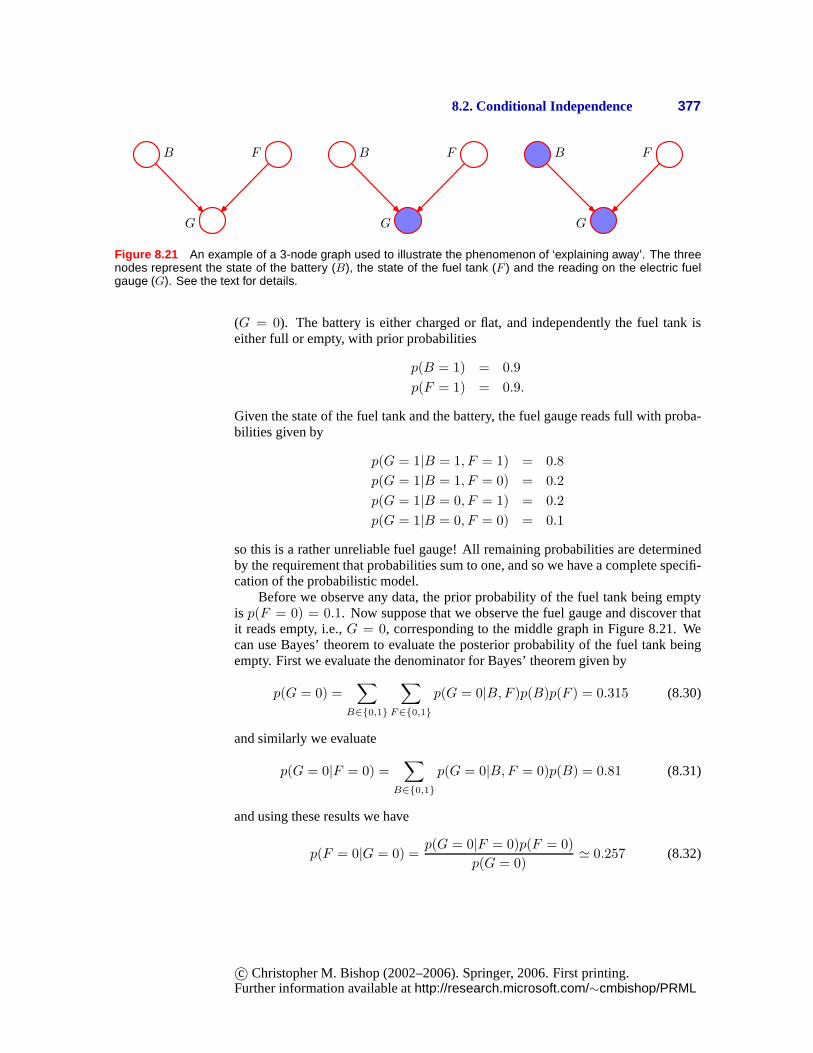
Figure 8.21 An example of a 3-node graph used to illustrate the phenomenon of ‘explaining away’. The threenodes represent the state of the battery (B), the state of the fuel tank (F ) and the reading on the electric fuelgauge (G). See the text for details.
(G = 0). The battery is either charged or flat, and independently the fuel tank iseither full or empty, with prior probabilities
p(B = 1) = 0.9
p(F = 1) = 0.9.
Given the state of the fuel tank and the battery, the fuel gauge reads full with proba-bilities given by
p(G = 1|B = 1, F = 1) = 0.8
p(G = 1|B = 1, F = 0) = 0.2
p(G = 1|B = 0, F = 1) = 0.2
p(G = 1|B = 0, F = 0) = 0.1
so this is a rather unreliable fuel gauge! All remaining probabilities are determinedby the requirement that probabilities sum to one, and so we have a complete specifi-cation of the probabilistic model.
Before we observe any data, the prior probability of the fueltank being emptyis p(F = 0) = 0.1. Now suppose that we observe the fuel gauge and discover thatit reads empty, i.e.,G = 0, corresponding to the middle graph in Figure 8.21. Wecan use Bayes’ theorem to evaluate the posterior probability of the fuel tank beingempty. First we evaluate the denominator for Bayes’ theoremgiven by
p(G = 0) =∑
B∈{0,1}
∑
F∈{0,1}
p(G = 0|B,F )p(B)p(F ) = 0.315 (8.30)
and similarly we evaluate
p(G = 0|F = 0) =∑
B∈{0,1}
p(G = 0|B,F = 0)p(B) = 0.81 (8.31)
and using these results we have
p(F = 0|G = 0) =p(G = 0|F = 0)p(F = 0)
p(G = 0)' 0.257 (8.32)
c© Christopher M. Bishop (2002–2006). Springer, 2006. First printing.Further information available athttp://research.microsoft.com/∼cmbishop/PRML
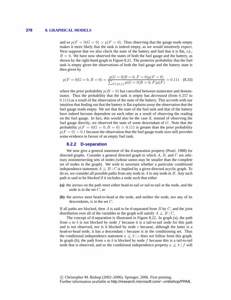
378 8. GRAPHICAL MODELS
and sop(F = 0|G = 0) > p(F = 0). Thus observing that the gauge reads emptymakes it more likely that the tank is indeed empty, as we wouldintuitively expect.Next suppose that we also check the state of the battery and find that it is flat, i.e.,B = 0. We have now observed the states of both the fuel gauge and thebattery, asshown by the right-hand graph in Figure 8.21. The posterior probability that the fueltank is empty given the observations of both the fuel gauge and the battery state isthen given by
p(F = 0|G = 0, B = 0) =p(G = 0|B = 0, F = 0)p(F = 0)∑
F∈{0,1} p(G = 0|B = 0, F )p(F )' 0.111 (8.33)
where the prior probabilityp(B = 0) has cancelled between numerator and denom-inator. Thus the probability that the tank is empty hasdecreased(from 0.257 to0.111) as a result of the observation of the state of the battery. This accords with ourintuition that finding out that the battery is flatexplains awaythe observation that thefuel gauge reads empty. We see that the state of the fuel tank and that of the batteryhave indeed become dependent on each other as a result of observing the readingon the fuel gauge. In fact, this would also be the case if, instead of observing thefuel gauge directly, we observed the state of some descendant of G. Note that theprobabilityp(F = 0|G = 0, B = 0) ' 0.111 is greater than the prior probabilityp(F = 0) = 0.1 because the observation that the fuel gauge reads zero stillprovidessome evidence in favour of an empty fuel tank.
8.2.2 D-separationWe now give a general statement of the d-separation property(Pearl, 1988) for
directed graphs. Consider a general directed graph in whichA, B, andC are arbi-trary nonintersecting sets of nodes (whose union may be smaller than the completeset of nodes in the graph). We wish to ascertain whether a particular conditionalindependence statementA ⊥⊥ B | C is implied by a given directed acyclic graph. Todo so, we consider all possible paths from any node inA to any node inB. Any suchpath is said to beblockedif it includes a node such that either
(a) the arrows on the path meet either head-to-tail or tail-to-tail at the node, and thenode is in the setC, or
(b) the arrows meet head-to-head at the node, and neither the node, nor any of itsdescendants, is in the setC.
If all paths are blocked, thenA is said to be d-separated fromB byC, and the jointdistribution over all of the variables in the graph will satisfyA ⊥⊥ B | C.
The concept of d-separation is illustrated in Figure 8.22. In graph (a), the pathfrom a to b is not blocked by nodef because it is a tail-to-tail node for this pathand is not observed, nor is it blocked by nodee because, although the latter is ahead-to-head node, it has a descendantc because is in the conditioning set. Thusthe conditional independence statementa ⊥⊥ b | c doesnot follow from this graph.In graph (b), the path froma to b is blocked by nodef because this is a tail-to-tailnode that is observed, and so the conditional independence propertya ⊥⊥ b | f will
c© Christopher M. Bishop (2002–2006). Springer, 2006. First printing.Further information available athttp://research.microsoft.com/∼cmbishop/PRML
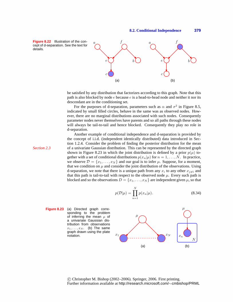
8.2. Conditional Independence 379
Figure 8.22 Illustration of the con-cept of d-separation. See the text fordetails.
f
e b
a
c
(a)
f
e b
a
c
(b)
be satisfied by any distribution that factorizes according to this graph. Note that thispath is also blocked by nodee becausee is a head-to-head node and neither it nor itsdescendant are in the conditioning set.
For the purposes of d-separation, parameters such asα andσ2 in Figure 8.5,indicated by small filled circles, behave in the same was as observed nodes. How-ever, there are no marginal distributions associated with such nodes. Consequentlyparameter nodes never themselves have parents and so all paths through these nodeswill always be tail-to-tail and hence blocked. Consequently they play no role ind-separation.
Another example of conditional independence and d-separation is provided bythe concept of i.i.d. (independent identically distributed) data introduced in Sec-tion 1.2.4. Consider the problem of finding the posterior distribution for the meanof a univariate Gaussian distribution. This can be represented by the directed graphSection 2.3shown in Figure 8.23 in which the joint distribution is defined by a priorp(µ) to-gether with a set of conditional distributionsp(xn|µ) for n = 1, . . . , N . In practice,we observeD = {x1, . . . , xN} and our goal is to inferµ. Suppose, for a moment,that we condition onµ and consider the joint distribution of the observations. Usingd-separation, we note that there is a unique path from anyxi to any otherxj 6=i andthat this path is tail-to-tail with respect to the observed nodeµ. Every such path isblocked and so the observationsD = {x1, . . . , xN} are independent givenµ, so that
p(D|µ) =
N∏
n=1
p(xn|µ). (8.34)
Figure 8.23 (a) Directed graph corre-sponding to the problemof inferring the mean µ ofa univariate Gaussian dis-tribution from observationsx1, . . . , xN . (b) The samegraph drawn using the platenotation.
µ
x1 xN
(a)
xn
N
N
µ
(b)
c© Christopher M. Bishop (2002–2006). Springer, 2006. First printing.Further information available athttp://research.microsoft.com/∼cmbishop/PRML
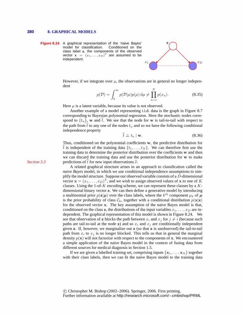
380 8. GRAPHICAL MODELS
Figure 8.24 A graphical representation of the ‘naive Bayes’model for classification. Conditioned on theclass label z, the components of the observedvector x = (x1, . . . , xD)T are assumed to beindependent.
z
x1 xD
However, if we integrate overµ, the observations are in general no longer indepen-dent
p(D) =
∫ ∞
0
p(D|µ)p(µ) dµ 6=N∏
n=1
p(xn). (8.35)
Hereµ is a latent variable, because its value is not observed.Another example of a model representing i.i.d. data is the graph in Figure 8.7
corresponding to Bayesian polynomial regression. Here thestochastic nodes corre-spond to{tn}, w and t. We see that the node forw is tail-to-tail with respect tothe path fromt to any one of the nodestn and so we have the following conditionalindependence property
t ⊥⊥ tn | w. (8.36)
Thus, conditioned on the polynomial coefficientsw, the predictive distribution fort is independent of the training data{t1, . . . , tN}. We can therefore first use thetraining data to determine the posterior distribution overthe coefficientsw and thenwe can discard the training data and use the posterior distribution for w to makepredictions oft for new input observationsx.Section 3.3
A related graphical structure arises in an approach to classification called thenaive Bayesmodel, in which we use conditional independence assumptions to sim-plify the model structure. Suppose our observed variable consists of aD-dimensionalvectorx = (x1, . . . , xD)T, and we wish to assign observed values ofx to one ofKclasses. Using the 1-of-K encoding scheme, we can represent these classes by aK-dimensional binary vectorz. We can then define a generative model by introducinga multinomial priorp(z|µ) over the class labels, where thekth componentµk of µ
is the prior probability of classCk, together with a conditional distributionp(x|z)for the observed vectorx. The key assumption of the naive Bayes model is that,conditioned on the classz, the distributions of the input variablesx1, . . . , xD are in-dependent. The graphical representation of this model is shown in Figure 8.24. Wesee that observation ofz blocks the path betweenxi andxj for j 6= i (because suchpaths are tail-to-tail at the nodez) and soxi andxj are conditionally independentgivenz. If, however, we marginalize outz (so thatz is unobserved) the tail-to-tailpath fromxi to xj is no longer blocked. This tells us that in general the marginaldensityp(x) will not factorize with respect to the components ofx. We encountereda simple application of the naive Bayes model in the context of fusing data fromdifferent sources for medical diagnosis in Section 1.5.
If we are given a labelled training set, comprising inputs{x1, . . . ,xN} togetherwith their class labels, then we can fit the naive Bayes model to the training data
c© Christopher M. Bishop (2002–2006). Springer, 2006. First printing.Further information available athttp://research.microsoft.com/∼cmbishop/PRML
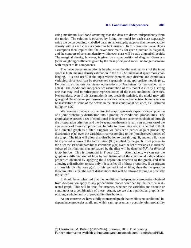
8.2. Conditional Independence 381
using maximum likelihood assuming that the data are drawn independently fromthe model. The solution is obtained by fitting the model for each class separatelyusing the correspondingly labelled data. As an example, suppose that the probabilitydensity within each class is chosen to be Gaussian. In this case, the naive Bayesassumption then implies that the covariance matrix for eachGaussian is diagonal,and the contours of constant density within each class will be axis-aligned ellipsoids.The marginal density, however, is given by a superposition of diagonal Gaussians(with weighting coefficients given by the class priors) and so will no longer factorizewith respect to its components.
The naive Bayes assumption is helpful when the dimensionality D of the inputspace is high, making density estimation in the fullD-dimensional space more chal-lenging. It is also useful if the input vector contains both discrete and continuousvariables, since each can be represented separately using appropriate models (e.g.,Bernoulli distributions for binary observations or Gaussians for real-valued vari-ables). The conditional independence assumption of this model is clearly a strongone that may lead to rather poor representations of the class-conditional densities.Nevertheless, even if this assumption is not precisely satisfied, the model may stillgive good classification performance in practice because the decision boundaries canbe insensitive to some of the details in the class-conditional densities, as illustratedin Figure 1.27.
We have seen that a particular directed graph represents a specific decompositionof a joint probability distribution into a product of conditional probabilities. Thegraph also expresses a set of conditional independence statements obtained throughthe d-separation criterion, and the d-separation theorem is really an expression of theequivalence of these two properties. In order to make this clear, it is helpful to thinkof a directed graph as a filter. Suppose we consider a particular joint probabilitydistributionp(x) over the variablesx corresponding to the (nonobserved) nodes ofthe graph. The filter will allow this distribution to pass through if, and only if, it canbe expressed in terms of the factorization (8.5) implied by the graph. If we present tothe filter the set of all possible distributionsp(x) over the set of variablesx, then thesubset of distributions that are passed by the filter will be denotedDF , for directedfactorization. This is illustrated in Figure 8.25. Alternatively, we can use thegraph as a different kind of filter by first listing all of the conditional independenceproperties obtained by applying the d-separation criterion to the graph, and thenallowing a distribution to pass only if it satisfies all of these properties. If we presentall possible distributionsp(x) to this second kind of filter, then the d-separationtheorem tells us that the set of distributions that will be allowed through is preciselythe setDF .
It should be emphasized that the conditional independence properties obtainedfrom d-separation apply to any probabilistic model described by that particular di-rected graph. This will be true, for instance, whether the variables are discrete orcontinuous or a combination of these. Again, we see that a particular graph is de-scribing a whole family of probability distributions.
At one extreme we have a fully connected graph that exhibits no conditional in-dependence properties at all, and which can represent any possible joint probability
c© Christopher M. Bishop (2002–2006). Springer, 2006. First printing.Further information available athttp://research.microsoft.com/∼cmbishop/PRML
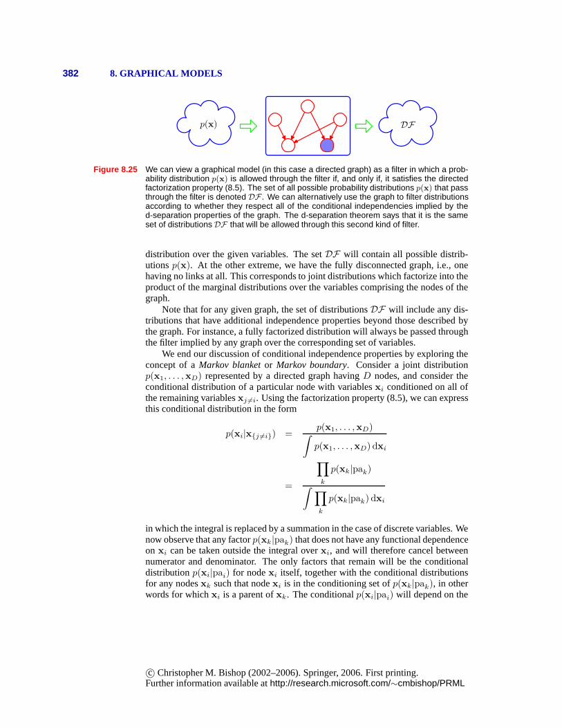
382 8. GRAPHICAL MODELS
p(x) DF
Figure 8.25 We can view a graphical model (in this case a directed graph) as a filter in which a prob-ability distribution p(x) is allowed through the filter if, and only if, it satisfies the directedfactorization property (8.5). The set of all possible probability distributions p(x) that passthrough the filter is denoted DF . We can alternatively use the graph to filter distributionsaccording to whether they respect all of the conditional independencies implied by thed-separation properties of the graph. The d-separation theorem says that it is the sameset of distributions DF that will be allowed through this second kind of filter.
distribution over the given variables. The setDF will contain all possible distrib-utionsp(x). At the other extreme, we have the fully disconnected graph,i.e., onehaving no links at all. This corresponds to joint distributions which factorize into theproduct of the marginal distributions over the variables comprising the nodes of thegraph.
Note that for any given graph, the set of distributionsDF will include any dis-tributions that have additional independence properties beyond those described bythe graph. For instance, a fully factorized distribution will always be passed throughthe filter implied by any graph over the corresponding set of variables.
We end our discussion of conditional independence properties by exploring theconcept of aMarkov blanketor Markov boundary. Consider a joint distributionp(x1, . . . ,xD) represented by a directed graph havingD nodes, and consider theconditional distribution of a particular node with variablesxi conditioned on all ofthe remaining variablesxj 6=i. Using the factorization property (8.5), we can expressthis conditional distribution in the form
p(xi|x{j 6=i}) =p(x1, . . . ,xD)∫p(x1, . . . ,xD) dxi
=
∏
k
p(xk|pak)
∫ ∏
k
p(xk|pak) dxi
in which the integral is replaced by a summation in the case ofdiscrete variables. Wenow observe that any factorp(xk|pak) that does not have any functional dependenceon xi can be taken outside the integral overxi, and will therefore cancel betweennumerator and denominator. The only factors that remain will be the conditionaldistributionp(xi|pai) for nodexi itself, together with the conditional distributionsfor any nodesxk such that nodexi is in the conditioning set ofp(xk|pak), in otherwords for whichxi is a parent ofxk. The conditionalp(xi|pai) will depend on the
c© Christopher M. Bishop (2002–2006). Springer, 2006. First printing.Further information available athttp://research.microsoft.com/∼cmbishop/PRML
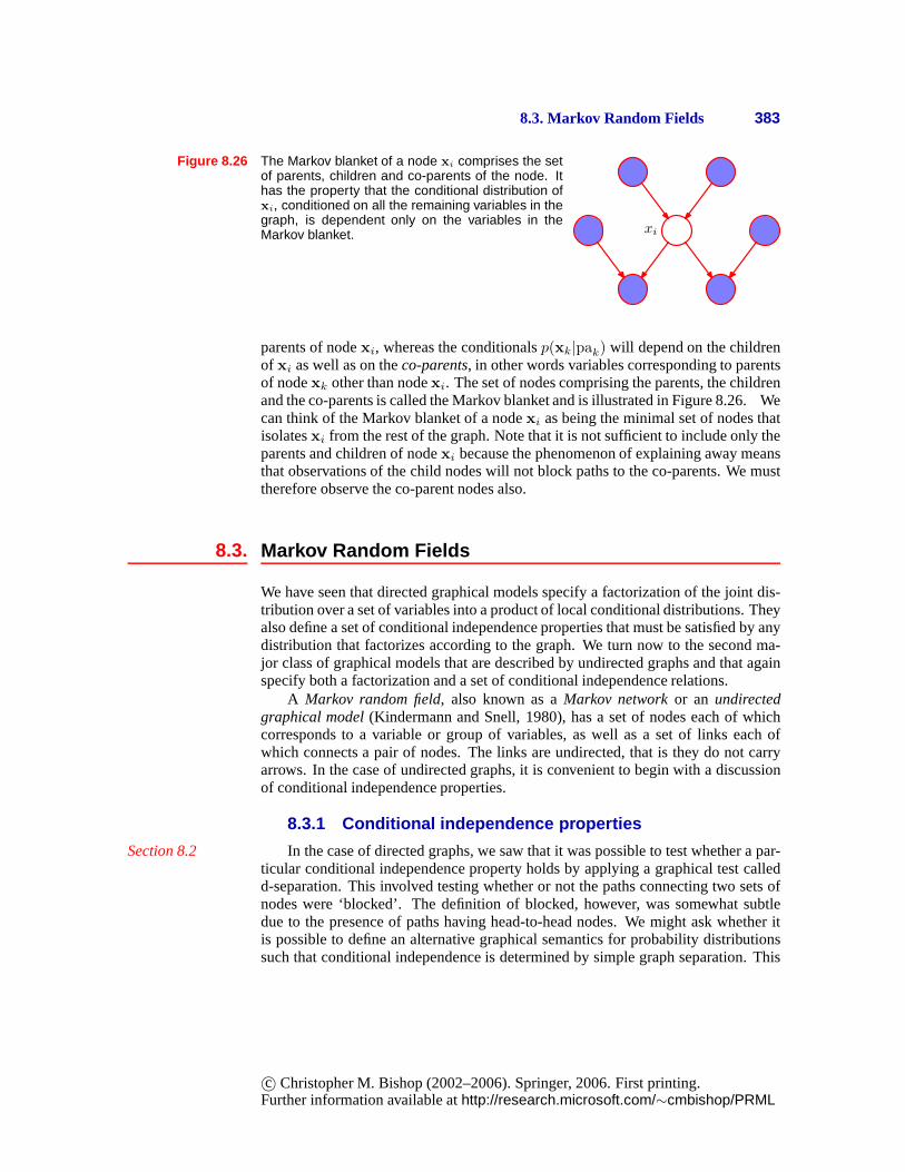
8.3. Markov Random Fields 383
Figure 8.26 The Markov blanket of a node xi comprises the setof parents, children and co-parents of the node. Ithas the property that the conditional distribution ofxi, conditioned on all the remaining variables in thegraph, is dependent only on the variables in theMarkov blanket. xi
parents of nodexi, whereas the conditionalsp(xk|pak) will depend on the childrenof xi as well as on theco-parents, in other words variables corresponding to parentsof nodexk other than nodexi. The set of nodes comprising the parents, the childrenand the co-parents is called the Markov blanket and is illustrated in Figure 8.26. Wecan think of the Markov blanket of a nodexi as being the minimal set of nodes thatisolatesxi from the rest of the graph. Note that it is not sufficient to include only theparents and children of nodexi because the phenomenon of explaining away meansthat observations of the child nodes will not block paths to the co-parents. We musttherefore observe the co-parent nodes also.
8.3. Markov Random Fields
We have seen that directed graphical models specify a factorization of the joint dis-tribution over a set of variables into a product of local conditional distributions. Theyalso define a set of conditional independence properties that must be satisfied by anydistribution that factorizes according to the graph. We turn now to the second ma-jor class of graphical models that are described by undirected graphs and that againspecify both a factorization and a set of conditional independence relations.
A Markov random field, also known as aMarkov networkor an undirectedgraphical model(Kindermann and Snell, 1980), has a set of nodes each of whichcorresponds to a variable or group of variables, as well as a set of links each ofwhich connects a pair of nodes. The links are undirected, that is they do not carryarrows. In the case of undirected graphs, it is convenient tobegin with a discussionof conditional independence properties.
8.3.1 Conditional independence properties
In the case of directed graphs, we saw that it was possible to test whether a par-Section 8.2ticular conditional independence property holds by applying a graphical test calledd-separation. This involved testing whether or not the paths connecting two sets ofnodes were ‘blocked’. The definition of blocked, however, was somewhat subtledue to the presence of paths having head-to-head nodes. We might ask whether itis possible to define an alternative graphical semantics forprobability distributionssuch that conditional independence is determined by simplegraph separation. This
c© Christopher M. Bishop (2002–2006). Springer, 2006. First printing.Further information available athttp://research.microsoft.com/∼cmbishop/PRML
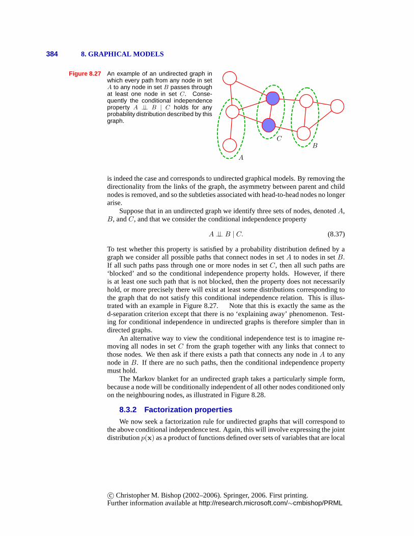
384 8. GRAPHICAL MODELS
Figure 8.27 An example of an undirected graph inwhich every path from any node in setA to any node in set B passes throughat least one node in set C. Conse-quently the conditional independenceproperty A ⊥⊥ B | C holds for anyprobability distribution described by thisgraph.
A
CB
is indeed the case and corresponds to undirected graphical models. By removing thedirectionality from the links of the graph, the asymmetry between parent and childnodes is removed, and so the subtleties associated with head-to-head nodes no longerarise.
Suppose that in an undirected graph we identify three sets ofnodes, denotedA,B, andC, and that we consider the conditional independence property
A ⊥⊥ B | C. (8.37)
To test whether this property is satisfied by a probability distribution defined by agraph we consider all possible paths that connect nodes in set A to nodes in setB.If all such paths pass through one or more nodes in setC, then all such paths are‘blocked’ and so the conditional independence property holds. However, if thereis at least one such path that is not blocked, then the property does not necessarilyhold, or more precisely there will exist at least some distributions corresponding tothe graph that do not satisfy this conditional independencerelation. This is illus-trated with an example in Figure 8.27. Note that this is exactly the same as thed-separation criterion except that there is no ‘explainingaway’ phenomenon. Test-ing for conditional independence in undirected graphs is therefore simpler than indirected graphs.
An alternative way to view the conditional independence test is to imagine re-moving all nodes in setC from the graph together with any links that connect tothose nodes. We then ask if there exists a path that connects any node inA to anynode inB. If there are no such paths, then the conditional independence propertymust hold.
The Markov blanket for an undirected graph takes a particularly simple form,because a node will be conditionally independent of all other nodes conditioned onlyon the neighbouring nodes, as illustrated in Figure 8.28.
8.3.2 Factorization propertiesWe now seek a factorization rule for undirected graphs that will correspond to
the above conditional independence test. Again, this will involve expressing the jointdistributionp(x) as a product of functions defined over sets of variables that are local
c© Christopher M. Bishop (2002–2006). Springer, 2006. First printing.Further information available athttp://research.microsoft.com/∼cmbishop/PRML
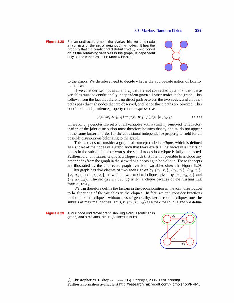
8.3. Markov Random Fields 385
Figure 8.28 For an undirected graph, the Markov blanket of a nodexi consists of the set of neighbouring nodes. It has theproperty that the conditional distribution of xi, conditionedon all the remaining variables in the graph, is dependentonly on the variables in the Markov blanket.
to the graph. We therefore need to decide what is the appropriate notion of localityin this case.
If we consider two nodesxi andxj that are not connected by a link, then thesevariables must be conditionally independent given all other nodes in the graph. Thisfollows from the fact that there is no direct path between thetwo nodes, and all otherpaths pass through nodes that are observed, and hence those paths are blocked. Thisconditional independence property can be expressed as
p(xi, xj|x\{i,j}) = p(xi|x\{i,j})p(xj|x\{i,j}) (8.38)
wherex\{i,j} denotes the setx of all variables withxi andxj removed. The factor-ization of the joint distribution must therefore be such that xi andxj do not appearin the same factor in order for the conditional independenceproperty to hold for allpossible distributions belonging to the graph.
This leads us to consider a graphical concept called aclique, which is definedas a subset of the nodes in a graph such that there exists a linkbetween all pairs ofnodes in the subset. In other words, the set of nodes in a clique is fully connected.Furthermore, amaximal cliqueis a clique such that it is not possible to include anyother nodes from the graph in the set without it ceasing to be aclique. These conceptsare illustrated by the undirected graph over four variablesshown in Figure 8.29.
This graph has five cliques of two nodes given by{x1, x2}, {x2, x3}, {x3, x4},{x4, x2}, and{x1, x3}, as well as two maximal cliques given by{x1, x2, x3} and{x2, x3, x4}. The set{x1, x2, x3, x4} is not a clique because of the missing linkfrom x1 to x4.
We can therefore define the factors in the decomposition of the joint distributionto be functions of the variables in the cliques. In fact, we can consider functionsof the maximal cliques, without loss of generality, becauseother cliques must besubsets of maximal cliques. Thus, if{x1, x2, x3} is a maximal clique and we define
Figure 8.29 A four-node undirected graph showing a clique (outlined ingreen) and a maximal clique (outlined in blue). x1
x2
x3
x4
c© Christopher M. Bishop (2002–2006). Springer, 2006. First printing.Further information available athttp://research.microsoft.com/∼cmbishop/PRML
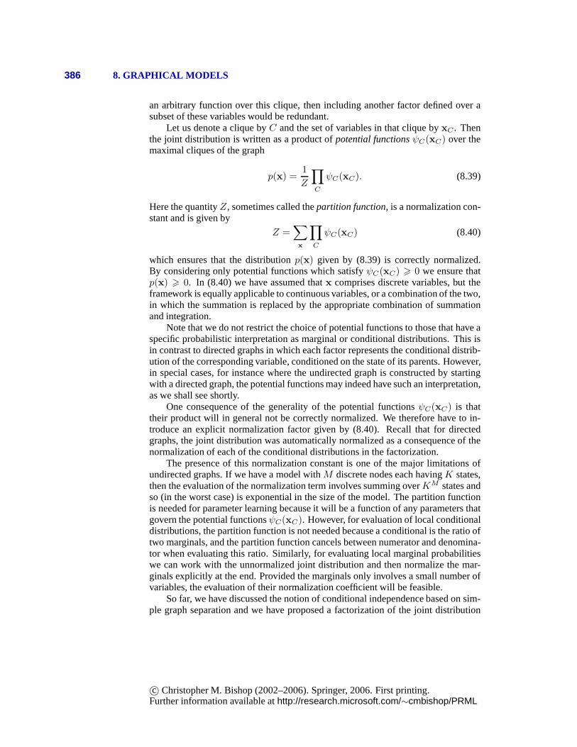
386 8. GRAPHICAL MODELS
an arbitrary function over this clique, then including another factor defined over asubset of these variables would be redundant.
Let us denote a clique byC and the set of variables in that clique byxC . Thenthe joint distribution is written as a product ofpotential functionsψC(xC) over themaximal cliques of the graph
p(x) =1
Z
∏
C
ψC(xC). (8.39)
Here the quantityZ, sometimes called thepartition function, is a normalization con-stant and is given by
Z =∑
x
∏
C
ψC(xC) (8.40)
which ensures that the distributionp(x) given by (8.39) is correctly normalized.By considering only potential functions which satisfyψC(xC) > 0 we ensure thatp(x) > 0. In (8.40) we have assumed thatx comprises discrete variables, but theframework is equally applicable to continuous variables, or a combination of the two,in which the summation is replaced by the appropriate combination of summationand integration.
Note that we do not restrict the choice of potential functions to those that have aspecific probabilistic interpretation as marginal or conditional distributions. This isin contrast to directed graphs in which each factor represents the conditional distrib-ution of the corresponding variable, conditioned on the state of its parents. However,in special cases, for instance where the undirected graph isconstructed by startingwith a directed graph, the potential functions may indeed have such an interpretation,as we shall see shortly.
One consequence of the generality of the potential functions ψC(xC) is thattheir product will in general not be correctly normalized. We therefore have to in-troduce an explicit normalization factor given by (8.40). Recall that for directedgraphs, the joint distribution was automatically normalized as a consequence of thenormalization of each of the conditional distributions in the factorization.
The presence of this normalization constant is one of the major limitations ofundirected graphs. If we have a model withM discrete nodes each havingK states,then the evaluation of the normalization term involves summing overKM states andso (in the worst case) is exponential in the size of the model.The partition functionis needed for parameter learning because it will be a function of any parameters thatgovern the potential functionsψC(xC). However, for evaluation of local conditionaldistributions, the partition function is not needed because a conditional is the ratio oftwo marginals, and the partition function cancels between numerator and denomina-tor when evaluating this ratio. Similarly, for evaluating local marginal probabilitieswe can work with the unnormalized joint distribution and then normalize the mar-ginals explicitly at the end. Provided the marginals only involves a small number ofvariables, the evaluation of their normalization coefficient will be feasible.
So far, we have discussed the notion of conditional independence based on sim-ple graph separation and we have proposed a factorization ofthe joint distribution
c© Christopher M. Bishop (2002–2006). Springer, 2006. First printing.Further information available athttp://research.microsoft.com/∼cmbishop/PRML
8.3. Markov Random Fields 387
that is intended to correspond to this conditional independence structure. However,we have not made any formal connection between conditional independence andfactorization for undirected graphs. To do so we need to restrict attention to poten-tial functionsψC(xC) that are strictly positive (i.e., never zero or negative foranychoice ofxC). Given this restriction, we can make a precise relationship betweenfactorization and conditional independence.
To do this we again return to the concept of a graphical model as a filter, corre-sponding to Figure 8.25. Consider the set of all possible distributions defined overa fixed set of variables corresponding to the nodes of a particular undirected graph.We can defineUI to be the set of such distributions that are consistent with the setof conditional independence statements that can be read from the graph using graphseparation. Similarly, we can defineUF to be the set of such distributions that canbe expressed as a factorization of the form (8.39) with respect to the maximal cliquesof the graph. TheHammersley-Cliffordtheorem (Clifford, 1990) states that the setsUI andUF are identical.
Because we are restricted to potential functions which are strictly positive it isconvenient to express them as exponentials, so that
ψC(xC) = exp {−E(xC)} (8.41)
whereE(xC) is called anenergy function, and the exponential representation iscalled theBoltzmann distribution. The joint distribution is defined as the product ofpotentials, and so the total energy is obtained by adding theenergies of each of themaximal cliques.
In contrast to the factors in the joint distribution for a directed graph, the po-tentials in an undirected graph do not have a specific probabilistic interpretation.Although this gives greater flexibility in choosing the potential functions, becausethere is no normalization constraint, it does raise the question of how to motivate achoice of potential function for a particular application.This can be done by view-ing the potential function as expressing which configurations of the local variablesare preferred to others. Global configurations that have a relatively high probabilityare those that find a good balance in satisfying the (possiblyconflicting) influencesof the clique potentials. We turn now to a specific example to illustrate the use ofundirected graphs.
8.3.3 Illustration: Image de-noising
We can illustrate the application of undirected graphs using an example of noiseremoval from a binary image (Besag, 1974; Geman and Geman, 1984; Besag, 1986).Although a very simple example, this is typical of more sophisticated applications.Let the observed noisy image be described by an array of binary pixel valuesyi ∈{−1,+1}, where the indexi = 1, . . . , D runs over all pixels. We shall supposethat the image is obtained by taking an unknown noise-free image, described bybinary pixel valuesxi ∈ {−1,+1} and randomly flipping the sign of pixels withsome small probability. An example binary image, together with a noise corruptedimage obtained by flipping the sign of the pixels with probability 10%, is shown in
c© Christopher M. Bishop (2002–2006). Springer, 2006. First printing.Further information available athttp://research.microsoft.com/∼cmbishop/PRML
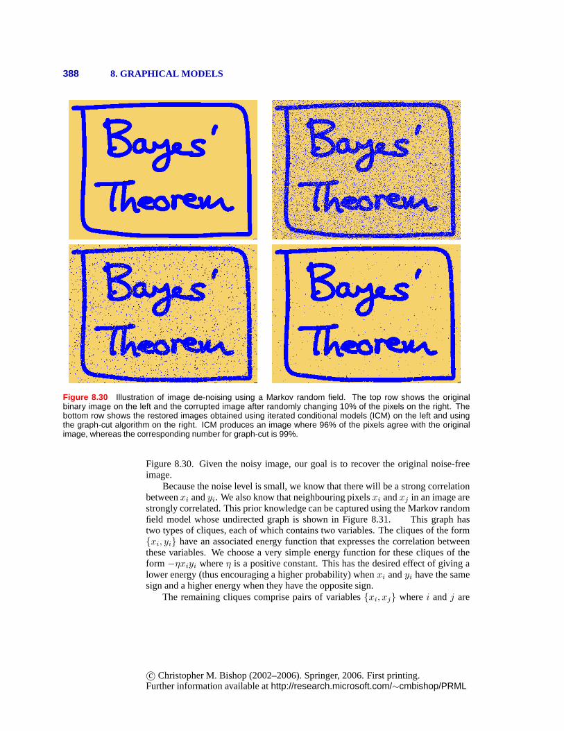
388 8. GRAPHICAL MODELS
Figure 8.30 Illustration of image de-noising using a Markov random field. The top row shows the originalbinary image on the left and the corrupted image after randomly changing 10% of the pixels on the right. Thebottom row shows the restored images obtained using iterated conditional models (ICM) on the left and usingthe graph-cut algorithm on the right. ICM produces an image where 96% of the pixels agree with the originalimage, whereas the corresponding number for graph-cut is 99%.
Figure 8.30. Given the noisy image, our goal is to recover theoriginal noise-freeimage.
Because the noise level is small, we know that there will be a strong correlationbetweenxi andyi. We also know that neighbouring pixelsxi andxj in an image arestrongly correlated. This prior knowledge can be captured using the Markov randomfield model whose undirected graph is shown in Figure 8.31. This graph hastwo types of cliques, each of which contains two variables. The cliques of the form{xi, yi} have an associated energy function that expresses the correlation betweenthese variables. We choose a very simple energy function forthese cliques of theform −ηxiyi whereη is a positive constant. This has the desired effect of givingalower energy (thus encouraging a higher probability) whenxi andyi have the samesign and a higher energy when they have the opposite sign.
The remaining cliques comprise pairs of variables{xi, xj} wherei andj are
c© Christopher M. Bishop (2002–2006). Springer, 2006. First printing.Further information available athttp://research.microsoft.com/∼cmbishop/PRML
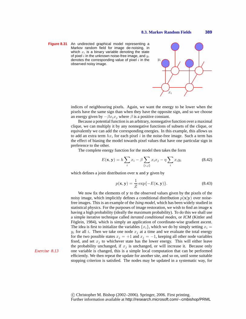
8.3. Markov Random Fields 389
Figure 8.31 An undirected graphical model representing aMarkov random field for image de-noising, inwhich xi is a binary variable denoting the stateof pixel i in the unknown noise-free image, and yi
denotes the corresponding value of pixel i in theobserved noisy image.
xi
yi
indices of neighbouring pixels. Again, we want the energy tobe lower when thepixels have the same sign than when they have the opposite sign, and so we choosean energy given by−βxixj whereβ is a positive constant.
Because a potential function is an arbitrary, nonnegative function over a maximalclique, we can multiply it by any nonnegative functions of subsets of the clique, orequivalently we can add the corresponding energies. In thisexample, this allows usto add an extra termhxi for each pixeli in the noise-free image. Such a term hasthe effect of biasing the model towards pixel values that have one particular sign inpreference to the other.
The complete energy function for the model then takes the form
E(x,y) = h∑
i
xi − β∑
{i,j}
xixj − η∑
i
xiyi (8.42)
which defines a joint distribution overx andy given by
p(x,y) =1
Zexp{−E(x,y)}. (8.43)
We now fix the elements ofy to the observed values given by the pixels of thenoisy image, which implicitly defines a conditional distribution p(x|y) over noise-free images. This is an example of theIsing model, which has been widely studied instatistical physics. For the purposes of image restoration, we wish to find an imagexhaving a high probability (ideally the maximum probability). To do this we shall usea simple iterative technique callediterated conditional modes, or ICM (Kittler andFoglein, 1984), which is simply an application of coordinate-wise gradient ascent.The idea is first to initialize the variables{xi}, which we do by simply settingxi =yi for all i. Then we take one nodexj at a time and we evaluate the total energyfor the two possible statesxj = +1 andxj = −1, keeping all other node variablesfixed, and setxj to whichever state has the lower energy. This will either leavethe probability unchanged, ifxj is unchanged, or will increase it. Because onlyone variable is changed, this is a simple local computation that can be performedExercise 8.13efficiently. We then repeat the update for another site, and so on, until some suitablestopping criterion is satisfied. The nodes may be updated in asystematic way, for
c© Christopher M. Bishop (2002–2006). Springer, 2006. First printing.Further information available athttp://research.microsoft.com/∼cmbishop/PRML
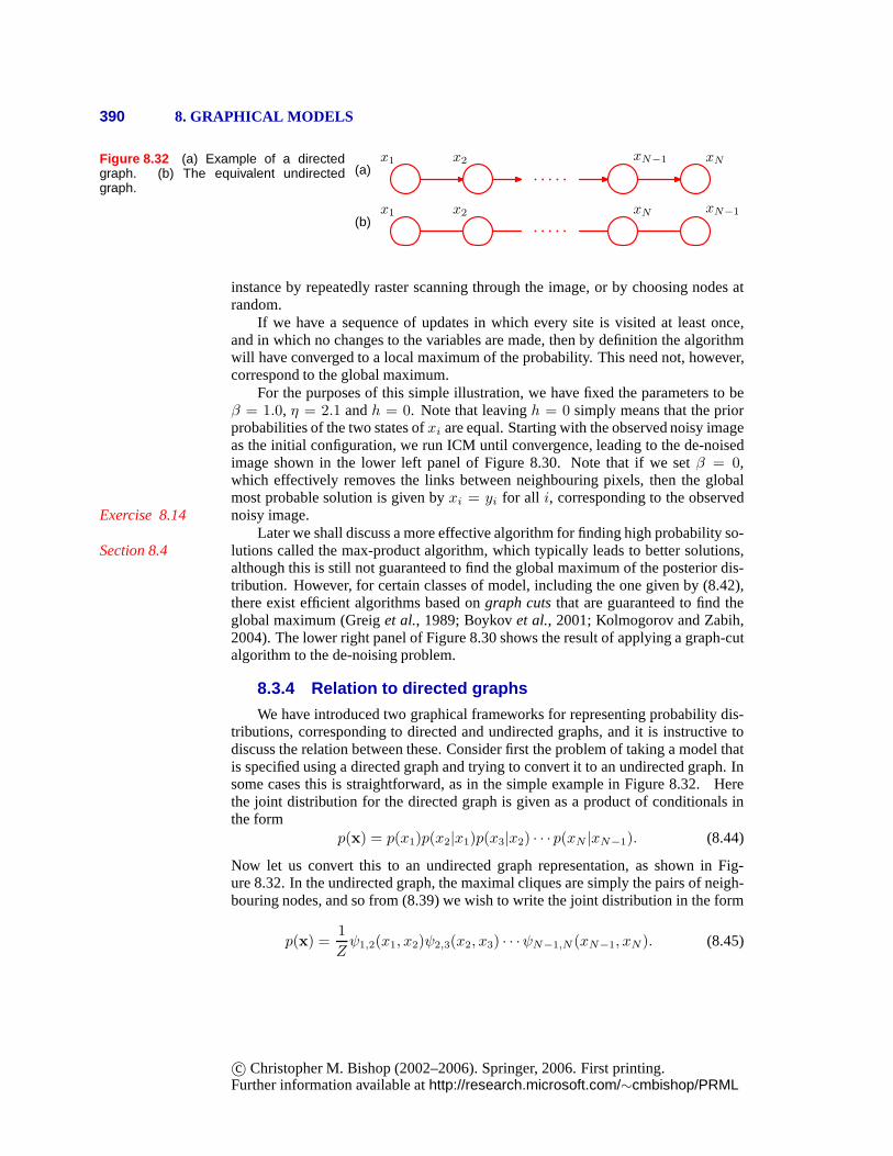
390 8. GRAPHICAL MODELS
Figure 8.32 (a) Example of a directedgraph. (b) The equivalent undirectedgraph.
(a)x1 x2 xN−1 xN
(b)x1 x2 xN−1xN
instance by repeatedly raster scanning through the image, or by choosing nodes atrandom.
If we have a sequence of updates in which every site is visitedat least once,and in which no changes to the variables are made, then by definition the algorithmwill have converged to a local maximum of the probability. This need not, however,correspond to the global maximum.
For the purposes of this simple illustration, we have fixed the parameters to beβ = 1.0, η = 2.1 andh = 0. Note that leavingh = 0 simply means that the priorprobabilities of the two states ofxi are equal. Starting with the observed noisy imageas the initial configuration, we run ICM until convergence, leading to the de-noisedimage shown in the lower left panel of Figure 8.30. Note that if we setβ = 0,which effectively removes the links between neighbouring pixels, then the globalmost probable solution is given byxi = yi for all i, corresponding to the observednoisy image.Exercise 8.14
Later we shall discuss a more effective algorithm for findinghigh probability so-lutions called the max-product algorithm, which typicallyleads to better solutions,Section 8.4although this is still not guaranteed to find the global maximum of the posterior dis-tribution. However, for certain classes of model, including the one given by (8.42),there exist efficient algorithms based ongraph cutsthat are guaranteed to find theglobal maximum (Greiget al., 1989; Boykovet al., 2001; Kolmogorov and Zabih,2004). The lower right panel of Figure 8.30 shows the result of applying a graph-cutalgorithm to the de-noising problem.
8.3.4 Relation to directed graphs
We have introduced two graphical frameworks for representing probability dis-tributions, corresponding to directed and undirected graphs, and it is instructive todiscuss the relation between these. Consider first the problem of taking a model thatis specified using a directed graph and trying to convert it toan undirected graph. Insome cases this is straightforward, as in the simple examplein Figure 8.32. Herethe joint distribution for the directed graph is given as a product of conditionals inthe form
p(x) = p(x1)p(x2|x1)p(x3|x2) · · · p(xN |xN−1). (8.44)
Now let us convert this to an undirected graph representation, as shown in Fig-ure 8.32. In the undirected graph, the maximal cliques are simply the pairs of neigh-bouring nodes, and so from (8.39) we wish to write the joint distribution in the form
p(x) =1
Zψ1,2(x1, x2)ψ2,3(x2, x3) · · ·ψN−1,N (xN−1, xN). (8.45)
c© Christopher M. Bishop (2002–2006). Springer, 2006. First printing.Further information available athttp://research.microsoft.com/∼cmbishop/PRML
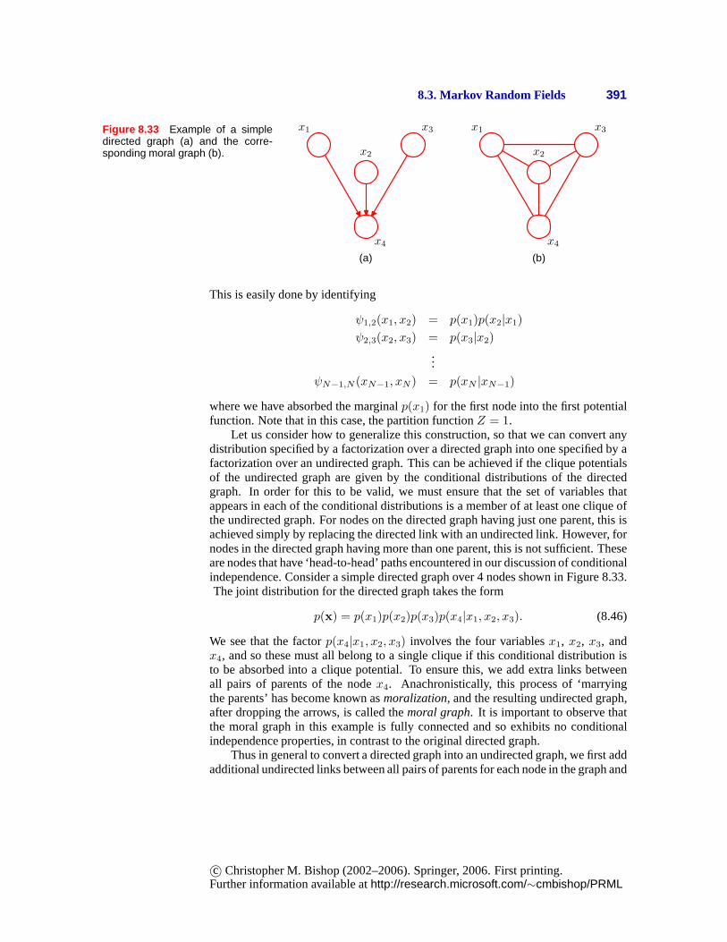
8.3. Markov Random Fields 391
Figure 8.33 Example of a simpledirected graph (a) and the corre-sponding moral graph (b).
x1 x3
x4
x2
(a)
x1 x3
x4
x2
(b)
This is easily done by identifying
ψ1,2(x1, x2) = p(x1)p(x2|x1)
ψ2,3(x2, x3) = p(x3|x2)
...
ψN−1,N (xN−1, xN) = p(xN |xN−1)
where we have absorbed the marginalp(x1) for the first node into the first potentialfunction. Note that in this case, the partition functionZ = 1.
Let us consider how to generalize this construction, so thatwe can convert anydistribution specified by a factorization over a directed graph into one specified by afactorization over an undirected graph. This can be achieved if the clique potentialsof the undirected graph are given by the conditional distributions of the directedgraph. In order for this to be valid, we must ensure that the set of variables thatappears in each of the conditional distributions is a memberof at least one clique ofthe undirected graph. For nodes on the directed graph havingjust one parent, this isachieved simply by replacing the directed link with an undirected link. However, fornodes in the directed graph having more than one parent, thisis not sufficient. Theseare nodes that have ‘head-to-head’ paths encountered in ourdiscussion of conditionalindependence. Consider a simple directed graph over 4 nodesshown in Figure 8.33.The joint distribution for the directed graph takes the form
p(x) = p(x1)p(x2)p(x3)p(x4|x1, x2, x3). (8.46)
We see that the factorp(x4|x1, x2, x3) involves the four variablesx1, x2, x3, andx4, and so these must all belong to a single clique if this conditional distribution isto be absorbed into a clique potential. To ensure this, we addextra links betweenall pairs of parents of the nodex4. Anachronistically, this process of ‘marryingthe parents’ has become known asmoralization, and the resulting undirected graph,after dropping the arrows, is called themoral graph. It is important to observe thatthe moral graph in this example is fully connected and so exhibits no conditionalindependence properties, in contrast to the original directed graph.
Thus in general to convert a directed graph into an undirected graph, we first addadditional undirected links between all pairs of parents for each node in the graph and
c© Christopher M. Bishop (2002–2006). Springer, 2006. First printing.Further information available athttp://research.microsoft.com/∼cmbishop/PRML
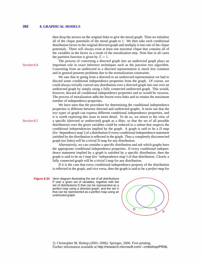
392 8. GRAPHICAL MODELS
then drop the arrows on the original links to give the moral graph. Then we initializeall of the clique potentials of the moral graph to 1. We then take each conditionaldistribution factor in the original directed graph and multiply it into one of the cliquepotentials. There will always exist at least one maximal clique that contains all ofthe variables in the factor as a result of the moralization step. Note that in all casesthe partition function is given byZ = 1.
The process of converting a directed graph into an undirected graph plays animportant role in exact inference techniques such as thejunction tree algorithm.Section 8.4Converting from an undirected to a directed representationis much less commonand in general presents problems due to the normalization constraints.
We saw that in going from a directed to an undirected representation we had todiscard some conditional independence properties from thegraph. Of course, wecould always trivially convert any distribution over a directed graph into one over anundirected graph by simply using a fully connected undirected graph. This would,however, discard all conditional independence propertiesand so would be vacuous.The process of moralization adds the fewest extra links and so retains the maximumnumber of independence properties.
We have seen that the procedure for determining the conditional independenceproperties is different between directed and undirected graphs. It turns out that thetwo types of graph can express different conditional independence properties, andit is worth exploring this issue in more detail. To do so, we return to the view ofa specific (directed or undirected) graph as a filter, so that the set of all possibleSection 8.2distributions over the given variables could be reduced to asubset that respects theconditional independencies implied by the graph. A graph issaid to be aD map(for ‘dependency map’) of a distribution if every conditional independence statementsatisfied by the distribution is reflected in the graph. Thus acompletely disconnectedgraph (no links) will be a trivial D map for any distribution.
Alternatively, we can consider a specific distribution and ask which graphs havethe appropriate conditional independence properties. If every conditional indepen-dence statement implied by a graph is satisfied by a specific distribution, then thegraph is said to be anI map(for ‘independence map’) of that distribution. Clearly afully connected graph will be a trivial I map for any distribution.
If it is the case that every conditional independence property of the distributionis reflected in the graph, and vice versa, then the graph is said to be aperfect mapfor
Figure 8.34 Venn diagram illustrating the set of all distributionsP over a given set of variables, together with theset of distributions D that can be represented as aperfect map using a directed graph, and the set Uthat can be represented as a perfect map using anundirected graph.
PUD
c© Christopher M. Bishop (2002–2006). Springer, 2006. First printing.Further information available athttp://research.microsoft.com/∼cmbishop/PRML
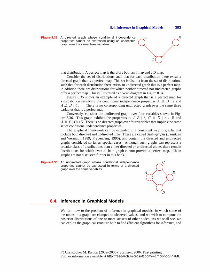
8.4. Inference in Graphical Models 393
Figure 8.35 A directed graph whose conditional independenceproperties cannot be expressed using an undirectedgraph over the same three variables.
C
A B
that distribution. A perfect map is therefore both an I map and a D map.Consider the set of distributions such that for each distribution there exists a
directed graph that is a perfect map. This set is distinct from the set of distributionssuch that for each distribution there exists an undirected graph that is a perfect map.In addition there are distributions for which neither directed nor undirected graphsoffer a perfect map. This is illustrated as a Venn diagram in Figure 8.34.
Figure 8.35 shows an example of a directed graph that is a perfect map fora distribution satisfying the conditional independence propertiesA ⊥⊥ B | ∅ andA 6⊥⊥ B | C. There is no corresponding undirected graph over the same threevariables that is a perfect map.
Conversely, consider the undirected graph over four variables shown in Fig-ure 8.36. This graph exhibits the propertiesA 6⊥⊥ B | ∅, C ⊥⊥ D | A ∪ B andA⊥⊥B | C∪D. There is no directed graph over four variables that impliesthe sameset of conditional independence properties.
The graphical framework can be extended in a consistent way to graphs thatinclude both directed and undirected links. These are called chain graphs(Lauritzenand Wermuth, 1989; Frydenberg, 1990), and contain the directed and undirectedgraphs considered so far as special cases. Although such graphs can represent abroader class of distributions than either directed or undirected alone, there remaindistributions for which even a chain graph cannot provide a perfect map. Chaingraphs are not discussed further in this book.
Figure 8.36 An undirected graph whose conditional independenceproperties cannot be expressed in terms of a directedgraph over the same variables.
A
C
B
D
8.4. Inference in Graphical Models
We turn now to the problem of inference in graphical models, in which some ofthe nodes in a graph are clamped to observed values, and we wish to compute theposterior distributions of one or more subsets of other nodes. As we shall see, wecan exploit the graphical structure both to find efficient algorithms for inference, and
c© Christopher M. Bishop (2002–2006). Springer, 2006. First printing.Further information available athttp://research.microsoft.com/∼cmbishop/PRML
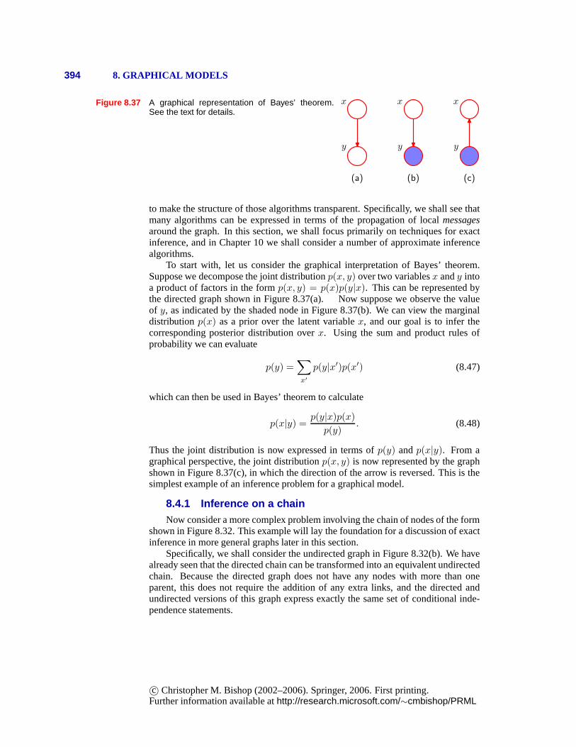
394 8. GRAPHICAL MODELS
Figure 8.37 A graphical representation of Bayes’ theorem.See the text for details.
x
y
x
y
x
y
(a) (b) (c)
to make the structure of those algorithms transparent. Specifically, we shall see thatmany algorithms can be expressed in terms of the propagationof local messagesaround the graph. In this section, we shall focus primarily on techniques for exactinference, and in Chapter 10 we shall consider a number of approximate inferencealgorithms.
To start with, let us consider the graphical interpretationof Bayes’ theorem.Suppose we decompose the joint distributionp(x, y) over two variablesx andy intoa product of factors in the formp(x, y) = p(x)p(y|x). This can be represented bythe directed graph shown in Figure 8.37(a). Now suppose we observe the valueof y, as indicated by the shaded node in Figure 8.37(b). We can view the marginaldistributionp(x) as a prior over the latent variablex, and our goal is to infer thecorresponding posterior distribution overx. Using the sum and product rules ofprobability we can evaluate
p(y) =∑
x′
p(y|x′)p(x′) (8.47)
which can then be used in Bayes’ theorem to calculate
p(x|y) =p(y|x)p(x)
p(y). (8.48)
Thus the joint distribution is now expressed in terms ofp(y) andp(x|y). From agraphical perspective, the joint distributionp(x, y) is now represented by the graphshown in Figure 8.37(c), in which the direction of the arrow is reversed. This is thesimplest example of an inference problem for a graphical model.
8.4.1 Inference on a chainNow consider a more complex problem involving the chain of nodes of the form
shown in Figure 8.32. This example will lay the foundation for a discussion of exactinference in more general graphs later in this section.
Specifically, we shall consider the undirected graph in Figure 8.32(b). We havealready seen that the directed chain can be transformed intoan equivalent undirectedchain. Because the directed graph does not have any nodes with more than oneparent, this does not require the addition of any extra links, and the directed andundirected versions of this graph express exactly the same set of conditional inde-pendence statements.
c© Christopher M. Bishop (2002–2006). Springer, 2006. First printing.Further information available athttp://research.microsoft.com/∼cmbishop/PRML
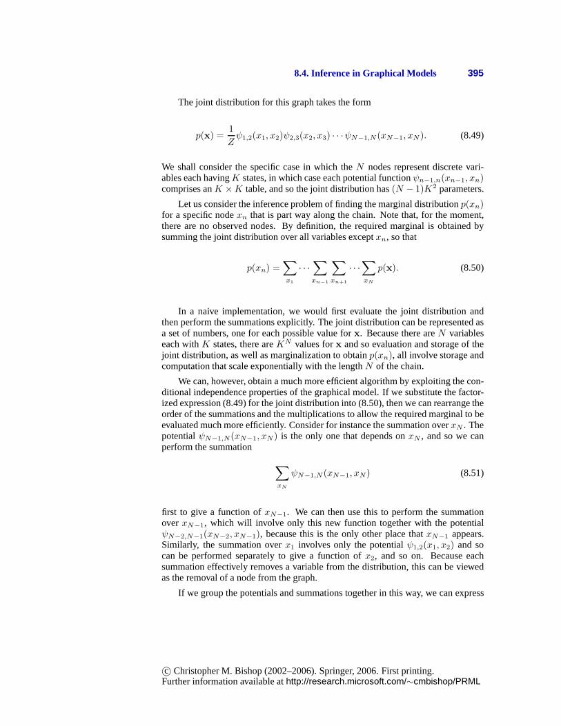
8.4. Inference in Graphical Models 395
The joint distribution for this graph takes the form
p(x) =1
Zψ1,2(x1, x2)ψ2,3(x2, x3) · · ·ψN−1,N (xN−1, xN). (8.49)
We shall consider the specific case in which theN nodes represent discrete vari-ables each havingK states, in which case each potential functionψn−1,n(xn−1, xn)comprises anK ×K table, and so the joint distribution has(N − 1)K2 parameters.
Let us consider the inference problem of finding the marginaldistributionp(xn)for a specific nodexn that is part way along the chain. Note that, for the moment,there are no observed nodes. By definition, the required marginal is obtained bysumming the joint distribution over all variables exceptxn, so that
p(xn) =∑
x1
· · ·∑
xn−1
∑
xn+1
· · ·∑
xN
p(x). (8.50)
In a naive implementation, we would first evaluate the joint distribution andthen perform the summations explicitly. The joint distribution can be represented asa set of numbers, one for each possible value forx. Because there areN variableseach withK states, there areKN values forx and so evaluation and storage of thejoint distribution, as well as marginalization to obtainp(xn), all involve storage andcomputation that scale exponentially with the lengthN of the chain.
We can, however, obtain a much more efficient algorithm by exploiting the con-ditional independence properties of the graphical model. If we substitute the factor-ized expression (8.49) for the joint distribution into (8.50), then we can rearrange theorder of the summations and the multiplications to allow therequired marginal to beevaluated much more efficiently. Consider for instance the summation overxN . ThepotentialψN−1,N(xN−1, xN) is the only one that depends onxN , and so we canperform the summation
∑
xN
ψN−1,N (xN−1, xN) (8.51)
first to give a function ofxN−1. We can then use this to perform the summationoverxN−1, which will involve only this new function together with thepotentialψN−2,N−1(xN−2, xN−1), because this is the only other place thatxN−1 appears.Similarly, the summation overx1 involves only the potentialψ1,2(x1, x2) and socan be performed separately to give a function ofx2, and so on. Because eachsummation effectively removes a variable from the distribution, this can be viewedas the removal of a node from the graph.
If we group the potentials and summations together in this way, we can express
c© Christopher M. Bishop (2002–2006). Springer, 2006. First printing.Further information available athttp://research.microsoft.com/∼cmbishop/PRML
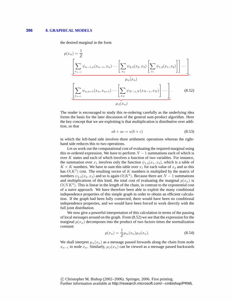
396 8. GRAPHICAL MODELS
the desired marginal in the form
p(xn) =1
Z∑
xn−1
ψn−1,n(xn−1, xn) · · ·[∑
x2
ψ2,3(x2, x3)
[∑
x1
ψ1,2(x1, x2)
]]· · ·
︸ ︷︷ ︸µα(xn)
∑
xn+1
ψn,n+1(xn, xn+1) · · ·[∑
xN
ψN−1,N(xN−1, xN )
]· · ·
︸ ︷︷ ︸µβ(xn)
. (8.52)
The reader is encouraged to study this re-ordering carefully as the underlying ideaforms the basis for the later discussion of the general sum-product algorithm. Herethe key concept that we are exploiting is that multiplication is distributive over addi-tion, so that
ab+ ac = a(b+ c) (8.53)
in which the left-hand side involves three arithmetic operations whereas the right-hand side reduces this to two operations.
Let us work out the computational cost of evaluating the required marginal usingthis re-ordered expression. We have to performN − 1 summations each of which isoverK states and each of which involves a function of two variables. For instance,the summation overx1 involves only the functionψ1,2(x1, x2), which is a table ofK ×K numbers. We have to sum this table overx1 for each value ofx2 and so thishasO(K2) cost. The resulting vector ofK numbers is multiplied by the matrix ofnumbersψ2,3(x2, x3) and so is againO(K2). Because there areN − 1 summationsand multiplications of this kind, the total cost of evaluating the marginalp(xn) isO(NK2). This is linear in the length of the chain, in contrast to the exponential costof a naive approach. We have therefore been able to exploit the many conditionalindependence properties of this simple graph in order to obtain an efficient calcula-tion. If the graph had been fully connected, there would havebeen no conditionalindependence properties, and we would have been forced to work directly with thefull joint distribution.
We now give a powerful interpretation of this calculation interms of the passingof localmessagesaround on the graph. From (8.52) we see that the expression for themarginalp(xn) decomposes into the product of two factors times the normalizationconstant
p(xn) =1
Zµα(xn)µβ(xn). (8.54)
We shall interpretµα(xn) as a message passed forwards along the chain from nodexn−1 to nodexn. Similarly,µβ(xn) can be viewed as a message passed backwards
c© Christopher M. Bishop (2002–2006). Springer, 2006. First printing.Further information available athttp://research.microsoft.com/∼cmbishop/PRML
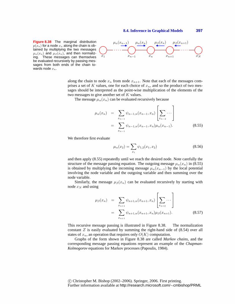
8.4. Inference in Graphical Models 397
Figure 8.38 The marginal distributionp(xn) for a node xn along the chain is ob-tained by multiplying the two messagesµα(xn) and µβ(xn), and then normaliz-ing. These messages can themselvesbe evaluated recursively by passing mes-sages from both ends of the chain to-wards node xn.
x1 xn−1 xn xn+1 xN
µα(xn−1) µα(xn) µβ(xn) µβ(xn+1)
along the chain to nodexn from nodexn+1. Note that each of the messages com-prises a set ofK values, one for each choice ofxn, and so the product of two mes-sages should be interpreted as the point-wise multiplication of the elements of thetwo messages to give another set ofK values.
The messageµα(xn) can be evaluated recursively because
µα(xn) =∑
xn−1
ψn−1,n(xn−1, xn)
∑
xn−2
· · ·
=∑
xn−1
ψn−1,n(xn−1, xn)µα(xn−1). (8.55)
We therefore first evaluate
µα(x2) =∑
x1
ψ1,2(x1, x2) (8.56)
and then apply (8.55) repeatedly until we reach the desired node. Note carefully thestructure of the message passing equation. The outgoing messageµα(xn) in (8.55)is obtained by multiplying the incoming messageµα(xn−1) by the local potentialinvolving the node variable and the outgoing variable and then summing over thenode variable.
Similarly, the messageµβ(xn) can be evaluated recursively by starting withnodexN and using
µβ(xn) =∑
xn+1
ψn+1,n(xn+1, xn)
∑
xn+2
· · ·
=∑
xn+1
ψn+1,n(xn+1, xn)µβ(xn+1). (8.57)
This recursive message passing is illustrated in Figure 8.38. The normalizationconstantZ is easily evaluated by summing the right-hand side of (8.54)over allstates ofxn, an operation that requires onlyO(K) computation.
Graphs of the form shown in Figure 8.38 are calledMarkov chains, and thecorresponding message passing equations represent an example of theChapman-Kolmogorovequations for Markov processes (Papoulis, 1984).
c© Christopher M. Bishop (2002–2006). Springer, 2006. First printing.Further information available athttp://research.microsoft.com/∼cmbishop/PRML
398 8. GRAPHICAL MODELS
Now suppose we wish to evaluate the marginalsp(xn) for every noden ∈{1, . . . , N} in the chain. Simply applying the above procedure separately for eachnode will have computational cost that isO(N 2M 2). However, such an approachwould be very wasteful of computation. For instance, to findp(x1) we need to prop-agate a messageµβ(·) from nodexN back to nodex2. Similarly, to evaluatep(x2)we need to propagate a messagesµβ(·) from nodexN back to nodex3. This willinvolve much duplicated computation because most of the messages will be identicalin the two cases.
Suppose instead we first launch a messageµβ(xN−1) starting from nodexN
and propagate corresponding messages all the way back to nodex1, and suppose wesimilarly launch a messageµα(x2) starting from nodex1 and propagate the corre-sponding messages all the way forward to nodexN . Provided we store all of theintermediate messages along the way, then any node can evaluate its marginal sim-ply by applying (8.54). The computational cost is only twicethat for finding themarginal of a single node, rather thanN times as much. Observe that a messagehas passed once in each direction across each link in the graph. Note also that thenormalization constantZ need be evaluated only once, using any convenient node.
If some of the nodes in the graph are observed, then the corresponding variablesare simply clamped to their observed values and there is no summation. To seethis, note that the effect of clamping a variablexn to an observed valuexn canbe expressed by multiplying the joint distribution by (one or more copies of) anadditional functionI(xn, xn), which takes the value1 whenxn = xn and the value0 otherwise. One such function can then be absorbed into each of the potentials thatcontainxn. Summations overxn then contain only one term in whichxn = xn.
Now suppose we wish to calculate the joint distributionp(xn−1, xn) for twoneighbouring nodes on the chain. This is similar to the evaluation of the marginalfor a single node, except that there are now two variables that are not summed out.A few moments thought will show that the required joint distribution can be writtenExercise 8.15in the form
p(xn−1, xn) =1
Zµα(xn−1)ψn−1,n(xn−1, xn)µβ(xn). (8.58)
Thus we can obtain the joint distributions over all of the sets of variables in eachof the potentials directly once we have completed the message passing required toobtain the marginals.
This is a useful result because in practice we may wish to use parametric formsfor the clique potentials, or equivalently for the conditional distributions if we startedfrom a directed graph. In order to learn the parameters of these potentials in situa-tions where not all of the variables are observed, we can employ theEM algorithm,Chapter 9and it turns out that the local joint distributions of the cliques, conditioned on anyobserved data, is precisely what is needed in the E step. We shall consider someexamples of this in detail in Chapter 13.
8.4.2 TreesWe have seen that exact inference on a graph comprising a chain of nodes can be
performed efficiently in time that is linear in the number of nodes, using an algorithm
c© Christopher M. Bishop (2002–2006). Springer, 2006. First printing.Further information available athttp://research.microsoft.com/∼cmbishop/PRML
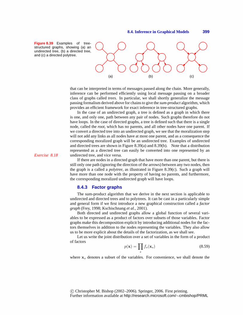
8.4. Inference in Graphical Models 399
Figure 8.39 Examples of tree-structured graphs, showing (a) anundirected tree, (b) a directed tree,and (c) a directed polytree.
(a) (b) (c)
that can be interpreted in terms of messages passed along thechain. More generally,inference can be performed efficiently using local message passing on a broaderclass of graphs calledtrees. In particular, we shall shortly generalize the messagepassing formalism derived above for chains to give thesum-productalgorithm, whichprovides an efficient framework for exact inference in tree-structured graphs.
In the case of an undirected graph, a tree is defined as a graph in which thereis one, and only one, path between any pair of nodes. Such graphs therefore do nothave loops. In the case of directed graphs, a tree is defined such that there is a singlenode, called theroot, which has no parents, and all other nodes have one parent. Ifwe convert a directed tree into an undirected graph, we see that the moralization stepwill not add any links as all nodes have at most one parent, andas a consequence thecorresponding moralized graph will be an undirected tree. Examples of undirectedand directed trees are shown in Figure 8.39(a) and 8.39(b). Note that a distributionrepresented as a directed tree can easily be converted into one represented by anundirected tree, and vice versa.Exercise 8.18
If there are nodes in a directed graph that have more than one parent, but there isstill only one path (ignoring the direction of the arrows) between any two nodes, thenthe graph is a called apolytree, as illustrated in Figure 8.39(c). Such a graph willhave more than one node with the property of having no parents, and furthermore,the corresponding moralized undirected graph will have loops.
8.4.3 Factor graphsThe sum-product algorithm that we derive in the next sectionis applicable to
undirected and directed trees and to polytrees. It can be cast in a particularly simpleand general form if we first introduce a new graphical construction called afactorgraph(Frey, 1998; Kschischnanget al., 2001).
Both directed and undirected graphs allow a global functionof several vari-ables to be expressed as a product of factors over subsets of those variables. Factorgraphs make this decomposition explicit by introducing additional nodes for the fac-tors themselves in addition to the nodes representing the variables. They also allowus to be more explicit about the details of the factorization, as we shall see.
Let us write the joint distribution over a set of variables inthe form of a productof factors
p(x) =∏
s
fs(xs) (8.59)
wherexs denotes a subset of the variables. For convenience, we shalldenote the
c© Christopher M. Bishop (2002–2006). Springer, 2006. First printing.Further information available athttp://research.microsoft.com/∼cmbishop/PRML
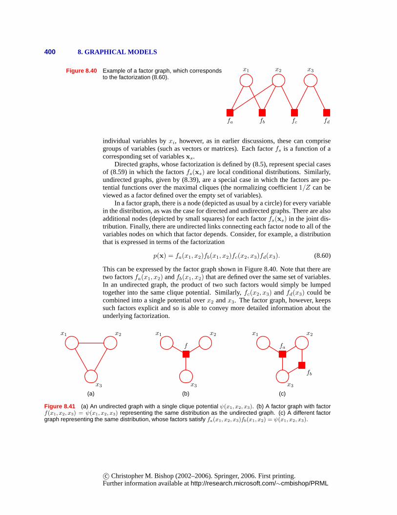
400 8. GRAPHICAL MODELS
Figure 8.40 Example of a factor graph, which correspondsto the factorization (8.60).
x1 x2 x3
fa fb fc fd
individual variables byxi, however, as in earlier discussions, these can comprisegroups of variables (such as vectors or matrices). Each factor fs is a function of acorresponding set of variablesxs.
Directed graphs, whose factorization is defined by (8.5), represent special casesof (8.59) in which the factorsfs(xs) are local conditional distributions. Similarly,undirected graphs, given by (8.39), are a special case in which the factors are po-tential functions over the maximal cliques (the normalizing coefficient1/Z can beviewed as a factor defined over the empty set of variables).
In a factor graph, there is a node (depicted as usual by a circle) for every variablein the distribution, as was the case for directed and undirected graphs. There are alsoadditional nodes (depicted by small squares) for each factor fs(xs) in the joint dis-tribution. Finally, there are undirected links connectingeach factor node to all of thevariables nodes on which that factor depends. Consider, forexample, a distributionthat is expressed in terms of the factorization
p(x) = fa(x1, x2)fb(x1, x2)fc(x2, x3)fd(x3). (8.60)
This can be expressed by the factor graph shown in Figure 8.40. Note that there aretwo factorsfa(x1, x2) andfb(x1, x2) that are defined over the same set of variables.In an undirected graph, the product of two such factors wouldsimply be lumpedtogether into the same clique potential. Similarly,fc(x2, x3) andfd(x3) could becombined into a single potential overx2 andx3. The factor graph, however, keepssuch factors explicit and so is able to convey more detailed information about theunderlying factorization.
x1 x2
x3
(a)
x1 x2
x3
f
(b)
x1 x2
x3
fa
fb
(c)
Figure 8.41 (a) An undirected graph with a single clique potential ψ(x1, x2, x3). (b) A factor graph with factorf(x1, x2, x3) = ψ(x1, x2, x3) representing the same distribution as the undirected graph. (c) A different factorgraph representing the same distribution, whose factors satisfy fa(x1, x2, x3)fb(x1, x2) = ψ(x1, x2, x3).
c© Christopher M. Bishop (2002–2006). Springer, 2006. First printing.Further information available athttp://research.microsoft.com/∼cmbishop/PRML
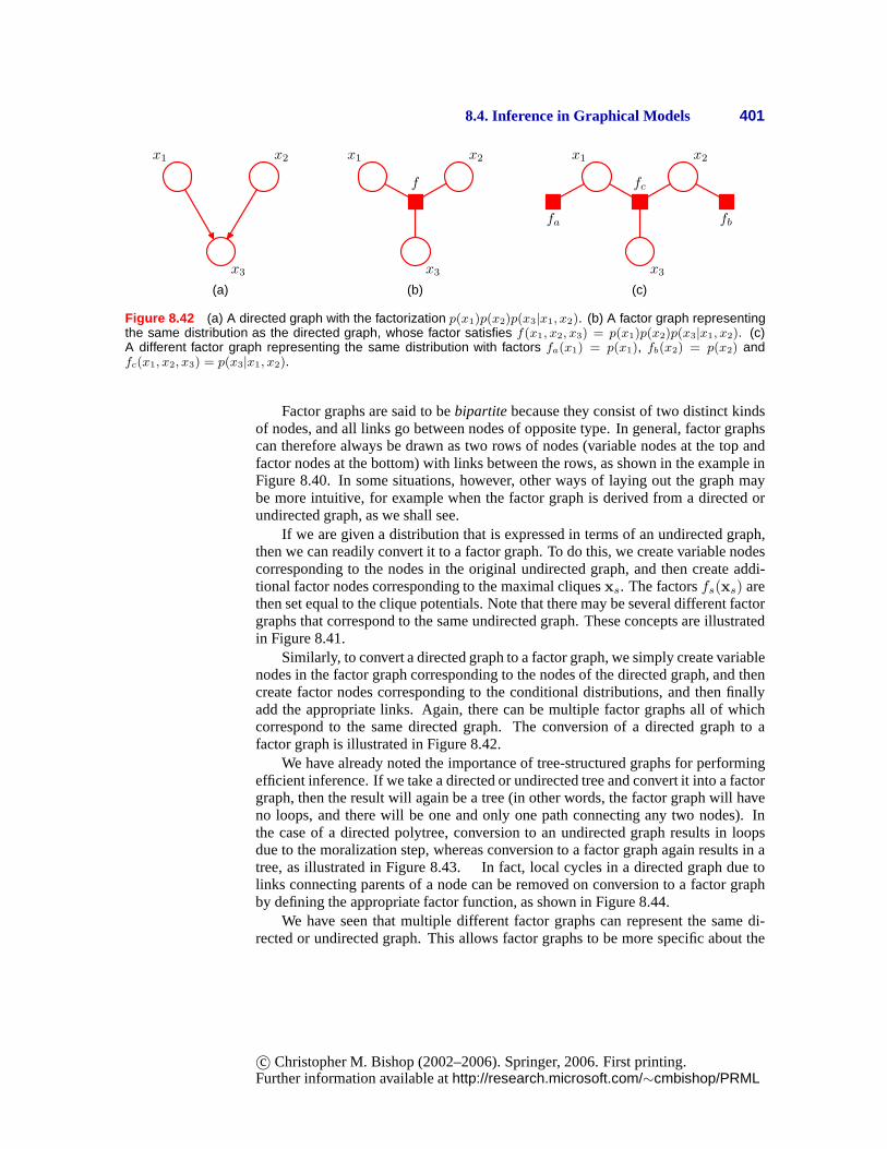
8.4. Inference in Graphical Models 401
x1 x2
x3
(a)
x1 x2
x3
f
(b)
x1 x2
x3
fc
fa fb
(c)
Figure 8.42 (a) A directed graph with the factorization p(x1)p(x2)p(x3|x1, x2). (b) A factor graph representingthe same distribution as the directed graph, whose factor satisfies f(x1, x2, x3) = p(x1)p(x2)p(x3|x1, x2). (c)A different factor graph representing the same distribution with factors fa(x1) = p(x1), fb(x2) = p(x2) andfc(x1, x2, x3) = p(x3|x1, x2).
Factor graphs are said to bebipartite because they consist of two distinct kindsof nodes, and all links go between nodes of opposite type. In general, factor graphscan therefore always be drawn as two rows of nodes (variable nodes at the top andfactor nodes at the bottom) with links between the rows, as shown in the example inFigure 8.40. In some situations, however, other ways of laying out the graph maybe more intuitive, for example when the factor graph is derived from a directed orundirected graph, as we shall see.
If we are given a distribution that is expressed in terms of anundirected graph,then we can readily convert it to a factor graph. To do this, wecreate variable nodescorresponding to the nodes in the original undirected graph, and then create addi-tional factor nodes corresponding to the maximal cliquesxs. The factorsfs(xs) arethen set equal to the clique potentials. Note that there may be several different factorgraphs that correspond to the same undirected graph. These concepts are illustratedin Figure 8.41.
Similarly, to convert a directed graph to a factor graph, we simply create variablenodes in the factor graph corresponding to the nodes of the directed graph, and thencreate factor nodes corresponding to the conditional distributions, and then finallyadd the appropriate links. Again, there can be multiple factor graphs all of whichcorrespond to the same directed graph. The conversion of a directed graph to afactor graph is illustrated in Figure 8.42.
We have already noted the importance of tree-structured graphs for performingefficient inference. If we take a directed or undirected treeand convert it into a factorgraph, then the result will again be a tree (in other words, the factor graph will haveno loops, and there will be one and only one path connecting any two nodes). Inthe case of a directed polytree, conversion to an undirectedgraph results in loopsdue to the moralization step, whereas conversion to a factorgraph again results in atree, as illustrated in Figure 8.43. In fact, local cycles ina directed graph due tolinks connecting parents of a node can be removed on conversion to a factor graphby defining the appropriate factor function, as shown in Figure 8.44.
We have seen that multiple different factor graphs can represent the same di-rected or undirected graph. This allows factor graphs to be more specific about the
c© Christopher M. Bishop (2002–2006). Springer, 2006. First printing.Further information available athttp://research.microsoft.com/∼cmbishop/PRML
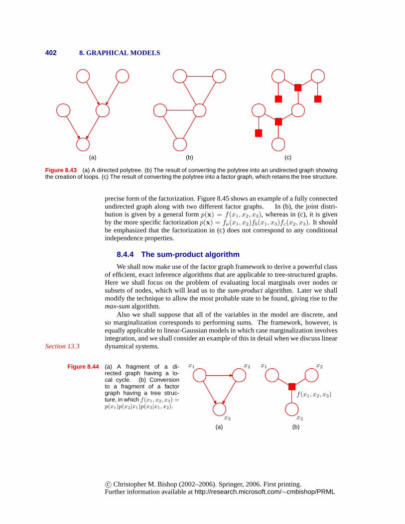
402 8. GRAPHICAL MODELS
(a) (b) (c)
Figure 8.43 (a) A directed polytree. (b) The result of converting the polytree into an undirected graph showingthe creation of loops. (c) The result of converting the polytree into a factor graph, which retains the tree structure.
precise form of the factorization. Figure 8.45 shows an example of a fully connectedundirected graph along with two different factor graphs. In(b), the joint distri-bution is given by a general formp(x) = f(x1, x2, x3), whereas in (c), it is givenby the more specific factorizationp(x) = fa(x1, x2)fb(x1, x3)fc(x2, x3). It shouldbe emphasized that the factorization in (c) does not correspond to any conditionalindependence properties.
8.4.4 The sum-product algorithm
We shall now make use of the factor graph framework to derive apowerful classof efficient, exact inference algorithms that are applicable to tree-structured graphs.Here we shall focus on the problem of evaluating local marginals over nodes orsubsets of nodes, which will lead us to thesum-productalgorithm. Later we shallmodify the technique to allow the most probable state to be found, giving rise to themax-sumalgorithm.
Also we shall suppose that all of the variables in the model are discrete, andso marginalization corresponds to performing sums. The framework, however, isequally applicable to linear-Gaussian models in which casemarginalization involvesintegration, and we shall consider an example of this in detail when we discuss lineardynamical systems.Section 13.3
Figure 8.44 (a) A fragment of a di-rected graph having a lo-cal cycle. (b) Conversionto a fragment of a factorgraph having a tree struc-ture, in which f(x1, x2, x3) =p(x1)p(x2|x1)p(x3|x1, x2).
x1 x2
x3
(a)
x1 x2
x3
f(x1, x2, x3)
(b)
c© Christopher M. Bishop (2002–2006). Springer, 2006. First printing.Further information available athttp://research.microsoft.com/∼cmbishop/PRML
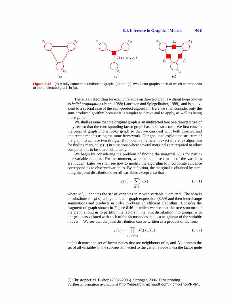
8.4. Inference in Graphical Models 403
x1 x2
x3
(a)
x1 x2
x3
f(x1, x2, x3)
(b)
x1 x2
x3
fa
fcfb
(c)
Figure 8.45 (a) A fully connected undirected graph. (b) and (c) Two factor graphs each of which correspondsto the undirected graph in (a).
There is an algorithm for exact inference on directed graphswithout loops knownasbelief propagation(Pearl, 1988; Lauritzen and Spiegelhalter, 1988), and is equiv-alent to a special case of the sum-product algorithm. Here weshall consider only thesum-product algorithm because it is simpler to derive and toapply, as well as beingmore general.
We shall assume that the original graph is an undirected treeor a directed tree orpolytree, so that the corresponding factor graph has a tree structure. We first convertthe original graph into a factor graph so that we can deal withboth directed andundirected models using the same framework. Our goal is to exploit the structure ofthe graph to achieve two things: (i) to obtain an efficient, exact inference algorithmfor finding marginals; (ii) in situations where several marginals are required to allowcomputations to be shared efficiently.
We begin by considering the problem of finding the marginalp(x) for partic-ular variable nodex. For the moment, we shall suppose that all of the variablesare hidden. Later we shall see how to modify the algorithm to incorporate evidencecorresponding to observed variables. By definition, the marginal is obtained by sum-ming the joint distribution over all variables exceptx so that
p(x) =∑
x\x
p(x) (8.61)
wherex \ x denotes the set of variables inx with variablex omitted. The idea isto substitute forp(x) using the factor graph expression (8.59) and then interchangesummations and products in order to obtain an efficient algorithm. Consider thefragment of graph shown in Figure 8.46 in which we see that thetree structure ofthe graph allows us to partition the factors in the joint distribution into groups, withone group associated with each of the factor nodes that is a neighbour of the variablenodex. We see that the joint distribution can be written as a product of the form
p(x) =∏
s∈ne(x)
Fs(x,Xs) (8.62)
ne(x) denotes the set of factor nodes that are neighbours ofx, andXs denotes theset of all variables in the subtree connected to the variablenodex via the factor node
c© Christopher M. Bishop (2002–2006). Springer, 2006. First printing.Further information available athttp://research.microsoft.com/∼cmbishop/PRML
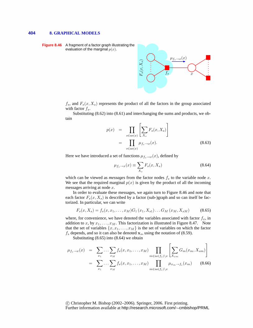
404 8. GRAPHICAL MODELS
Figure 8.46 A fragment of a factor graph illustrating theevaluation of the marginal p(x).
xfs
µfs→x(x)
Fs(x,X
s)
fs, andFs(x,Xs) represents the product of all the factors in the group associatedwith factorfs.
Substituting (8.62) into (8.61) and interchanging the sumsand products, we ob-tain
p(x) =∏
s∈ne(x)
[∑
Xs
Fs(x,Xs)
]
=∏
s∈ne(x)
µfs→x(x). (8.63)
Here we have introduced a set of functionsµfs→x(x), defined by
µfs→x(x) ≡∑
Xs
Fs(x,Xs) (8.64)
which can be viewed asmessagesfrom the factor nodesfs to the variable nodex.We see that the required marginalp(x) is given by the product of all the incomingmessages arriving at nodex.
In order to evaluate these messages, we again turn to Figure 8.46 and note thateach factorFs(x,Xs) is described by a factor (sub-)graph and so can itself be fac-torized. In particular, we can write
Fs(x,Xs) = fs(x, x1, . . . , xM )G1 (x1, Xs1) . . .GM (xM , XsM ) (8.65)
where, for convenience, we have denoted the variables associated with factorfx, inaddition tox, byx1, . . . , xM . This factorization is illustrated in Figure 8.47. Notethat the set of variables{x, x1, . . . , xM} is the set of variables on which the factorfs depends, and so it can also be denotedxs, using the notation of (8.59).
Substituting (8.65) into (8.64) we obtain
µfs→x(x) =∑
x1
. . .∑
xM
fs(x, x1, . . . , xM )∏
m∈ne(fs)\x
[∑
Xxm
Gm(xm, Xsm)
]
=∑
x1
. . .∑
xM
fs(x, x1, . . . , xM )∏
m∈ne(fs)\x
µxm→fs(xm) (8.66)
c© Christopher M. Bishop (2002–2006). Springer, 2006. First printing.Further information available athttp://research.microsoft.com/∼cmbishop/PRML
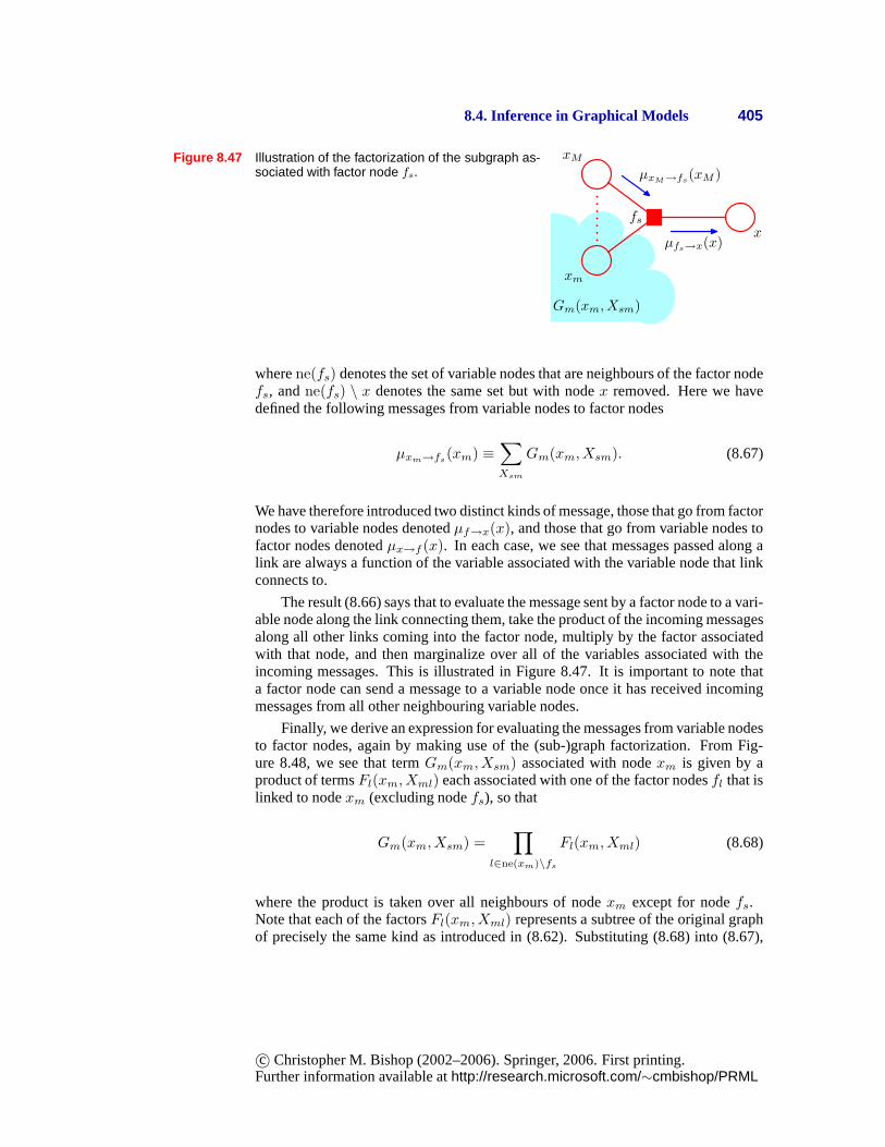
8.4. Inference in Graphical Models 405
Figure 8.47 Illustration of the factorization of the subgraph as-sociated with factor node fs.
xm
xM
xfs
µxM→fs(xM )
µfs→x(x)
Gm(xm, Xsm)
wherene(fs) denotes the set of variable nodes that are neighbours of the factor nodefs, andne(fs) \ x denotes the same set but with nodex removed. Here we havedefined the following messages from variable nodes to factornodes
µxm→fs(xm) ≡
∑
Xsm
Gm(xm, Xsm). (8.67)
We have therefore introduced two distinct kinds of message,those that go from factornodes to variable nodes denotedµf→x(x), and those that go from variable nodes tofactor nodes denotedµx→f (x). In each case, we see that messages passed along alink are always a function of the variable associated with the variable node that linkconnects to.
The result (8.66) says that to evaluate the message sent by a factor node to a vari-able node along the link connecting them, take the product ofthe incoming messagesalong all other links coming into the factor node, multiply by the factor associatedwith that node, and then marginalize over all of the variables associated with theincoming messages. This is illustrated in Figure 8.47. It isimportant to note thata factor node can send a message to a variable node once it has received incomingmessages from all other neighbouring variable nodes.
Finally, we derive an expression for evaluating the messages from variable nodesto factor nodes, again by making use of the (sub-)graph factorization. From Fig-ure 8.48, we see that termGm(xm, Xsm) associated with nodexm is given by aproduct of termsFl(xm, Xml) each associated with one of the factor nodesfl that islinked to nodexm (excluding nodefs), so that
Gm(xm, Xsm) =∏
l∈ne(xm)\fs
Fl(xm, Xml) (8.68)
where the product is taken over all neighbours of nodexm except for nodefs.Note that each of the factorsFl(xm, Xml) represents a subtree of the original graphof precisely the same kind as introduced in (8.62). Substituting (8.68) into (8.67),
c© Christopher M. Bishop (2002–2006). Springer, 2006. First printing.Further information available athttp://research.microsoft.com/∼cmbishop/PRML
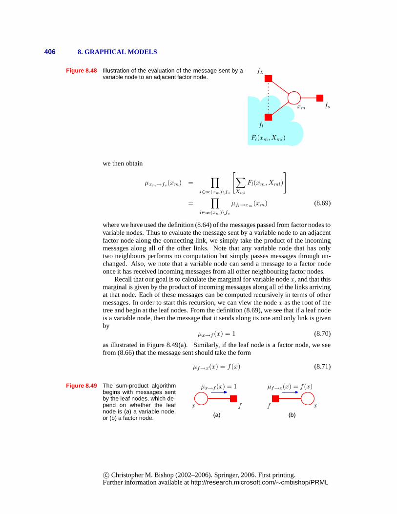
406 8. GRAPHICAL MODELS
Figure 8.48 Illustration of the evaluation of the message sent by avariable node to an adjacent factor node.
xm
fl
fL
fs
Fl(xm, Xml)
we then obtain
µxm→fs(xm) =
∏
l∈ne(xm)\fs
[∑
Xml
Fl(xm, Xml)
]
=∏
l∈ne(xm)\fs
µfl→xm(xm) (8.69)
where we have used the definition (8.64) of the messages passed from factor nodes tovariable nodes. Thus to evaluate the message sent by a variable node to an adjacentfactor node along the connecting link, we simply take the product of the incomingmessages along all of the other links. Note that any variablenode that has onlytwo neighbours performs no computation but simply passes messages through un-changed. Also, we note that a variable node can send a messageto a factor nodeonce it has received incoming messages from all other neighbouring factor nodes.
Recall that our goal is to calculate the marginal for variable nodex, and that thismarginal is given by the product of incoming messages along all of the links arrivingat that node. Each of these messages can be computed recursively in terms of othermessages. In order to start this recursion, we can view the nodex as the root of thetree and begin at the leaf nodes. From the definition (8.69), we see that if a leaf nodeis a variable node, then the message that it sends along its one and only link is givenby
µx→f (x) = 1 (8.70)
as illustrated in Figure 8.49(a). Similarly, if the leaf node is a factor node, we seefrom (8.66) that the message sent should take the form
µf→x(x) = f(x) (8.71)
Figure 8.49 The sum-product algorithmbegins with messages sentby the leaf nodes, which de-pend on whether the leafnode is (a) a variable node,or (b) a factor node.
x f
µx→f (x) = 1
(a)
xf
µf→x(x) = f(x)
(b)
c© Christopher M. Bishop (2002–2006). Springer, 2006. First printing.Further information available athttp://research.microsoft.com/∼cmbishop/PRML
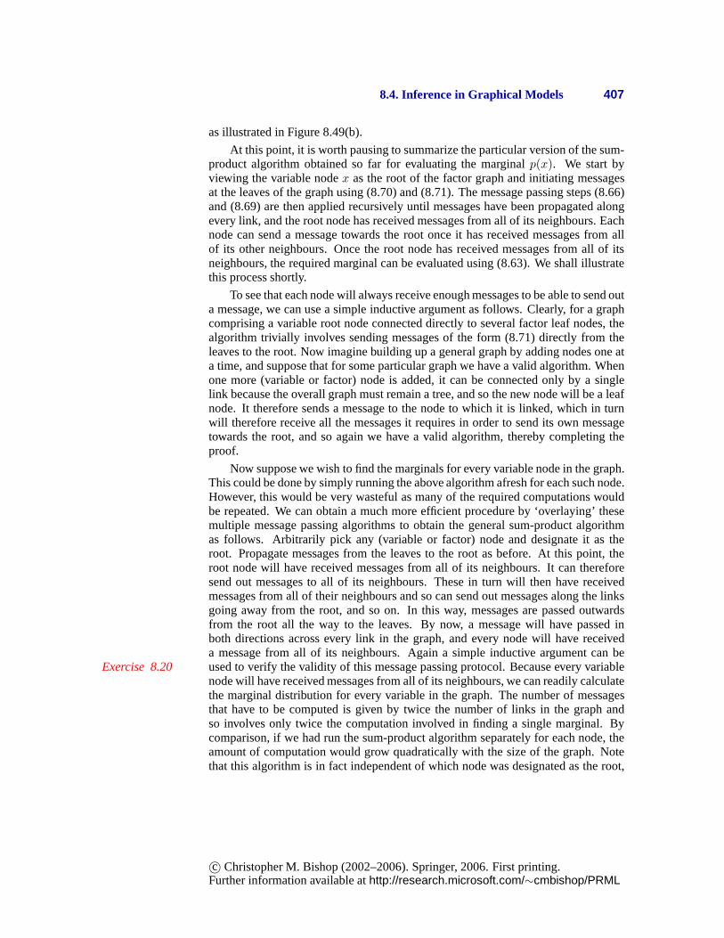
8.4. Inference in Graphical Models 407
as illustrated in Figure 8.49(b).
At this point, it is worth pausing to summarize the particular version of the sum-product algorithm obtained so far for evaluating the marginal p(x). We start byviewing the variable nodex as the root of the factor graph and initiating messagesat the leaves of the graph using (8.70) and (8.71). The message passing steps (8.66)and (8.69) are then applied recursively until messages havebeen propagated alongevery link, and the root node has received messages from all of its neighbours. Eachnode can send a message towards the root once it has received messages from allof its other neighbours. Once the root node has received messages from all of itsneighbours, the required marginal can be evaluated using (8.63). We shall illustratethis process shortly.
To see that each node will always receive enough messages to be able to send outa message, we can use a simple inductive argument as follows.Clearly, for a graphcomprising a variable root node connected directly to several factor leaf nodes, thealgorithm trivially involves sending messages of the form (8.71) directly from theleaves to the root. Now imagine building up a general graph byadding nodes one ata time, and suppose that for some particular graph we have a valid algorithm. Whenone more (variable or factor) node is added, it can be connected only by a singlelink because the overall graph must remain a tree, and so the new node will be a leafnode. It therefore sends a message to the node to which it is linked, which in turnwill therefore receive all the messages it requires in orderto send its own messagetowards the root, and so again we have a valid algorithm, thereby completing theproof.
Now suppose we wish to find the marginals for every variable node in the graph.This could be done by simply running the above algorithm afresh for each such node.However, this would be very wasteful as many of the required computations wouldbe repeated. We can obtain a much more efficient procedure by ‘overlaying’ thesemultiple message passing algorithms to obtain the general sum-product algorithmas follows. Arbitrarily pick any (variable or factor) node and designate it as theroot. Propagate messages from the leaves to the root as before. At this point, theroot node will have received messages from all of its neighbours. It can thereforesend out messages to all of its neighbours. These in turn willthen have receivedmessages from all of their neighbours and so can send out messages along the linksgoing away from the root, and so on. In this way, messages are passed outwardsfrom the root all the way to the leaves. By now, a message will have passed inboth directions across every link in the graph, and every node will have receiveda message from all of its neighbours. Again a simple inductive argument can beused to verify the validity of this message passing protocol. Because every variableExercise 8.20node will have received messages from all of its neighbours,we can readily calculatethe marginal distribution for every variable in the graph. The number of messagesthat have to be computed is given by twice the number of links in the graph andso involves only twice the computation involved in finding a single marginal. Bycomparison, if we had run the sum-product algorithm separately for each node, theamount of computation would grow quadratically with the size of the graph. Notethat this algorithm is in fact independent of which node was designated as the root,
c© Christopher M. Bishop (2002–2006). Springer, 2006. First printing.Further information available athttp://research.microsoft.com/∼cmbishop/PRML
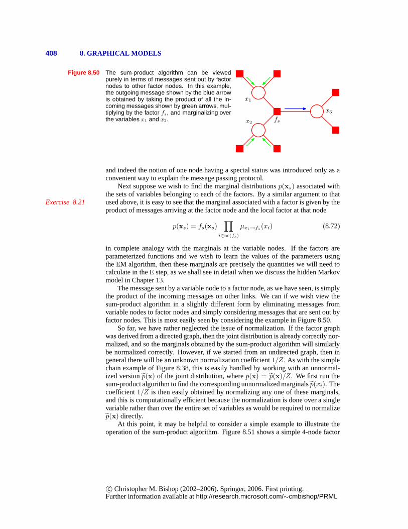
408 8. GRAPHICAL MODELS
Figure 8.50 The sum-product algorithm can be viewedpurely in terms of messages sent out by factornodes to other factor nodes. In this example,the outgoing message shown by the blue arrowis obtained by taking the product of all the in-coming messages shown by green arrows, mul-tiplying by the factor fs, and marginalizing overthe variables x1 and x2. fs
x1
x2
x3
and indeed the notion of one node having a special status was introduced only as aconvenient way to explain the message passing protocol.
Next suppose we wish to find the marginal distributionsp(xs) associated withthe sets of variables belonging to each of the factors. By a similar argument to thatused above, it is easy to see that the marginal associated with a factor is given by theExercise 8.21product of messages arriving at the factor node and the localfactor at that node
p(xs) = fs(xs)∏
i∈ne(fs)
µxi→fs(xi) (8.72)
in complete analogy with the marginals at the variable nodes. If the factors areparameterized functions and we wish to learn the values of the parameters usingthe EM algorithm, then these marginals are precisely the quantities we will need tocalculate in the E step, as we shall see in detail when we discuss the hidden Markovmodel in Chapter 13.
The message sent by a variable node to a factor node, as we haveseen, is simplythe product of the incoming messages on other links. We can ifwe wish view thesum-product algorithm in a slightly different form by eliminating messages fromvariable nodes to factor nodes and simply considering messages that are sent out byfactor nodes. This is most easily seen by considering the example in Figure 8.50.
So far, we have rather neglected the issue of normalization.If the factor graphwas derived from a directed graph, then the joint distribution is already correctly nor-malized, and so the marginals obtained by the sum-product algorithm will similarlybe normalized correctly. However, if we started from an undirected graph, then ingeneral there will be an unknown normalization coefficient1/Z. As with the simplechain example of Figure 8.38, this is easily handled by working with an unnormal-ized versionp(x) of the joint distribution, wherep(x) = p(x)/Z. We first run thesum-product algorithm to find the corresponding unnormalized marginalsp(xi). Thecoefficient1/Z is then easily obtained by normalizing any one of these marginals,and this is computationally efficient because the normalization is done over a singlevariable rather than over the entire set of variables as would be required to normalizep(x) directly.
At this point, it may be helpful to consider a simple example to illustrate theoperation of the sum-product algorithm. Figure 8.51 shows asimple 4-node factor
c© Christopher M. Bishop (2002–2006). Springer, 2006. First printing.Further information available athttp://research.microsoft.com/∼cmbishop/PRML
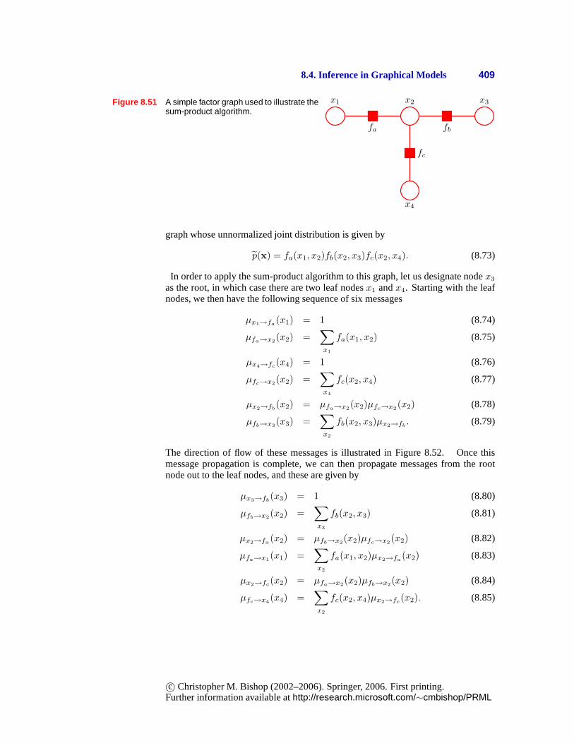
8.4. Inference in Graphical Models 409
Figure 8.51 A simple factor graph used to illustrate thesum-product algorithm.
x1 x2 x3
x4
fa fb
fc
graph whose unnormalized joint distribution is given by
p(x) = fa(x1, x2)fb(x2, x3)fc(x2, x4). (8.73)
In order to apply the sum-product algorithm to this graph, let us designate nodex3
as the root, in which case there are two leaf nodesx1 andx4. Starting with the leafnodes, we then have the following sequence of six messages
µx1→fa(x1) = 1 (8.74)
µfa→x2(x2) =
∑
x1
fa(x1, x2) (8.75)
µx4→fc(x4) = 1 (8.76)
µfc→x2(x2) =
∑
x4
fc(x2, x4) (8.77)
µx2→fb(x2) = µfa→x2
(x2)µfc→x2(x2) (8.78)
µfb→x3(x3) =
∑
x2
fb(x2, x3)µx2→fb. (8.79)
The direction of flow of these messages is illustrated in Figure 8.52. Once thismessage propagation is complete, we can then propagate messages from the rootnode out to the leaf nodes, and these are given by
µx3→fb(x3) = 1 (8.80)
µfb→x2(x2) =
∑
x3
fb(x2, x3) (8.81)
µx2→fa(x2) = µfb→x2
(x2)µfc→x2(x2) (8.82)
µfa→x1(x1) =
∑
x2
fa(x1, x2)µx2→fa(x2) (8.83)
µx2→fc(x2) = µfa→x2
(x2)µfb→x2(x2) (8.84)
µfc→x4(x4) =
∑
x2
fc(x2, x4)µx2→fc(x2). (8.85)
c© Christopher M. Bishop (2002–2006). Springer, 2006. First printing.Further information available athttp://research.microsoft.com/∼cmbishop/PRML
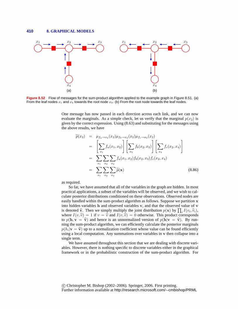
410 8. GRAPHICAL MODELS
x1 x2 x3
x4
(a)
x1 x2 x3
x4
(b)
Figure 8.52 Flow of messages for the sum-product algorithm applied to the example graph in Figure 8.51. (a)From the leaf nodes x1 and x4 towards the root node x3. (b) From the root node towards the leaf nodes.
One message has now passed in each direction across each link, and we can nowevaluate the marginals. As a simple check, let us verify thatthe marginalp(x2) isgiven by the correct expression. Using (8.63) and substituting for the messages usingthe above results, we have
p(x2) = µfa→x2(x2)µfb→x2
(x2)µfc→x2(x2)
=
[∑
x1
fa(x1, x2)
][∑
x3
fb(x2, x3)
][∑
x4
fc(x2, x4)
]
=∑
x1
∑
x2
∑
x4
fa(x1, x2)fb(x2, x3)fc(x2, x4)
=∑
x1
∑
x3
∑
x4
p(x) (8.86)
as required.So far, we have assumed that all of the variables in the graph are hidden. In most
practical applications, a subset of the variables will be observed, and we wish to cal-culate posterior distributions conditioned on these observations. Observed nodes areeasily handled within the sum-product algorithm as follows. Suppose we partitionxinto hidden variablesh and observed variablesv, and that the observed value ofv
is denotedv. Then we simply multiply the joint distributionp(x) by∏
i I(vi, vi),whereI(v, v) = 1 if v = v andI(v, v) = 0 otherwise. This product correspondsto p(h,v = v) and hence is an unnormalized version ofp(h|v = v). By run-ning the sum-product algorithm, we can efficiently calculate the posterior marginalsp(hi|v = v) up to a normalization coefficient whose value can be found efficientlyusing a local computation. Any summations over variables inv then collapse into asingle term.
We have assumed throughout this section that we are dealing with discrete vari-ables. However, there is nothing specific to discrete variables either in the graphicalframework or in the probabilistic construction of the sum-product algorithm. For
c© Christopher M. Bishop (2002–2006). Springer, 2006. First printing.Further information available athttp://research.microsoft.com/∼cmbishop/PRML
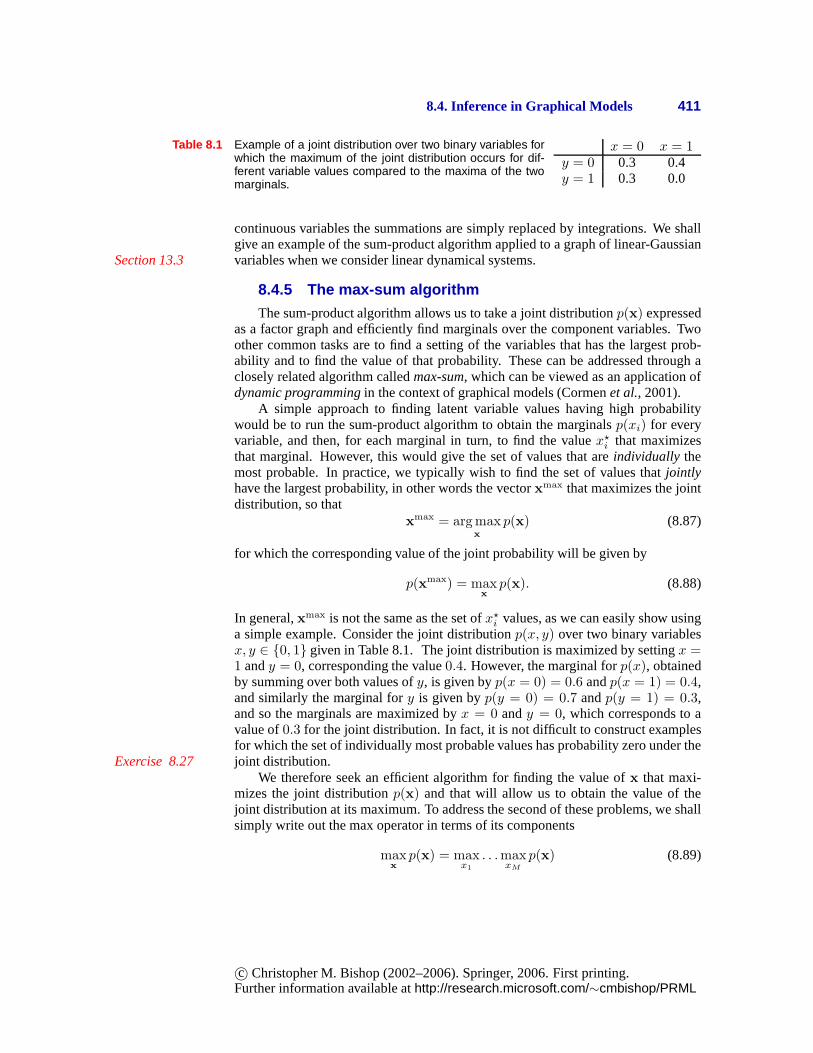
8.4. Inference in Graphical Models 411
Table 8.1 Example of a joint distribution over two binary variables forwhich the maximum of the joint distribution occurs for dif-ferent variable values compared to the maxima of the twomarginals.
x = 0 x = 1y = 0 0.3 0.4y = 1 0.3 0.0
continuous variables the summations are simply replaced byintegrations. We shallgive an example of the sum-product algorithm applied to a graph of linear-Gaussianvariables when we consider linear dynamical systems.Section 13.3
8.4.5 The max-sum algorithm
The sum-product algorithm allows us to take a joint distribution p(x) expressedas a factor graph and efficiently find marginals over the component variables. Twoother common tasks are to find a setting of the variables that has the largest prob-ability and to find the value of that probability. These can beaddressed through aclosely related algorithm calledmax-sum, which can be viewed as an application ofdynamic programmingin the context of graphical models (Cormenet al., 2001).
A simple approach to finding latent variable values having high probabilitywould be to run the sum-product algorithm to obtain the marginalsp(xi) for everyvariable, and then, for each marginal in turn, to find the value x?
i that maximizesthat marginal. However, this would give the set of values that are individually themost probable. In practice, we typically wish to find the set of values thatjointlyhave the largest probability, in other words the vectorxmax that maximizes the jointdistribution, so that
xmax = arg maxx
p(x) (8.87)
for which the corresponding value of the joint probability will be given by
p(xmax) = maxx
p(x). (8.88)
In general,xmax is not the same as the set ofx?i values, as we can easily show using
a simple example. Consider the joint distributionp(x, y) over two binary variablesx, y ∈ {0, 1} given in Table 8.1. The joint distribution is maximized by setting x =1 andy = 0, corresponding the value0.4. However, the marginal forp(x), obtainedby summing over both values ofy, is given byp(x = 0) = 0.6 andp(x = 1) = 0.4,and similarly the marginal fory is given byp(y = 0) = 0.7 andp(y = 1) = 0.3,and so the marginals are maximized byx = 0 andy = 0, which corresponds to avalue of0.3 for the joint distribution. In fact, it is not difficult to construct examplesfor which the set of individually most probable values has probability zero under thejoint distribution.Exercise 8.27
We therefore seek an efficient algorithm for finding the valueof x that maxi-mizes the joint distributionp(x) and that will allow us to obtain the value of thejoint distribution at its maximum. To address the second of these problems, we shallsimply write out the max operator in terms of its components
maxx
p(x) = maxx1
. . .maxxM
p(x) (8.89)
c© Christopher M. Bishop (2002–2006). Springer, 2006. First printing.Further information available athttp://research.microsoft.com/∼cmbishop/PRML
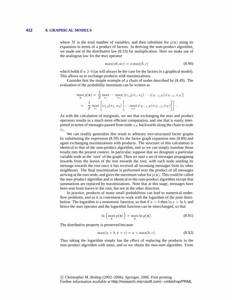
412 8. GRAPHICAL MODELS
whereM is the total number of variables, and then substitute forp(x) using itsexpansion in terms of a product of factors. In deriving the sum-product algorithm,we made use of the distributive law (8.53) for multiplication. Here we make use ofthe analogous law for the max operator
max(ab, ac) = amax(b, c) (8.90)
which holds ifa > 0 (as will always be the case for the factors in a graphical model).This allows us to exchange products with maximizations.
Consider first the simple example of a chain of nodes described by (8.49). Theevaluation of the probability maximum can be written as
maxx
p(x) =1
Zmax
x1
· · ·maxxN
[ψ1,2(x1, x2) · · ·ψN−1,N (xN−1, xN )]
=1
Zmax
x1
[ψ1,2(x1, x2)
[· · ·max
xN
ψN−1,N (xN−1, xN )
]].
As with the calculation of marginals, we see that exchangingthe max and productoperators results in a much more efficient computation, and one that is easily inter-preted in terms of messages passed from nodexN backwards along the chain to nodex1.
We can readily generalize this result to arbitrary tree-structured factor graphsby substituting the expression (8.59) for the factor graph expansion into (8.89) andagain exchanging maximizations with products. The structure of this calculation isidentical to that of the sum-product algorithm, and so we cansimply translate thoseresults into the present context. In particular, suppose that we designate a particularvariable node as the ‘root’ of the graph. Then we start a set ofmessages propagatinginwards from the leaves of the tree towards the root, with each node sending itsmessage towards the root once it has received all incoming messages from its otherneighbours. The final maximization is performed over the product of all messagesarriving at the root node, and gives the maximum value forp(x). This could be calledthemax-productalgorithm and is identical to the sum-product algorithm except thatsummations are replaced by maximizations. Note that at thisstage, messages havebeen sent from leaves to the root, but not in the other direction.
In practice, products of many small probabilities can lead to numerical under-flow problems, and so it is convenient to work with the logarithm of the joint distri-bution. The logarithm is a monotonic function, so that ifa > b thenln a > ln b, andhence the max operator and the logarithm function can be interchanged, so that
ln(max
x
p(x))
= maxx
ln p(x). (8.91)
The distributive property is preserved because
max(a+ b, a+ c) = a+ max(b, c). (8.92)
Thus taking the logarithm simply has the effect of replacingthe products in themax-product algorithm with sums, and so we obtain themax-sumalgorithm. From
c© Christopher M. Bishop (2002–2006). Springer, 2006. First printing.Further information available athttp://research.microsoft.com/∼cmbishop/PRML
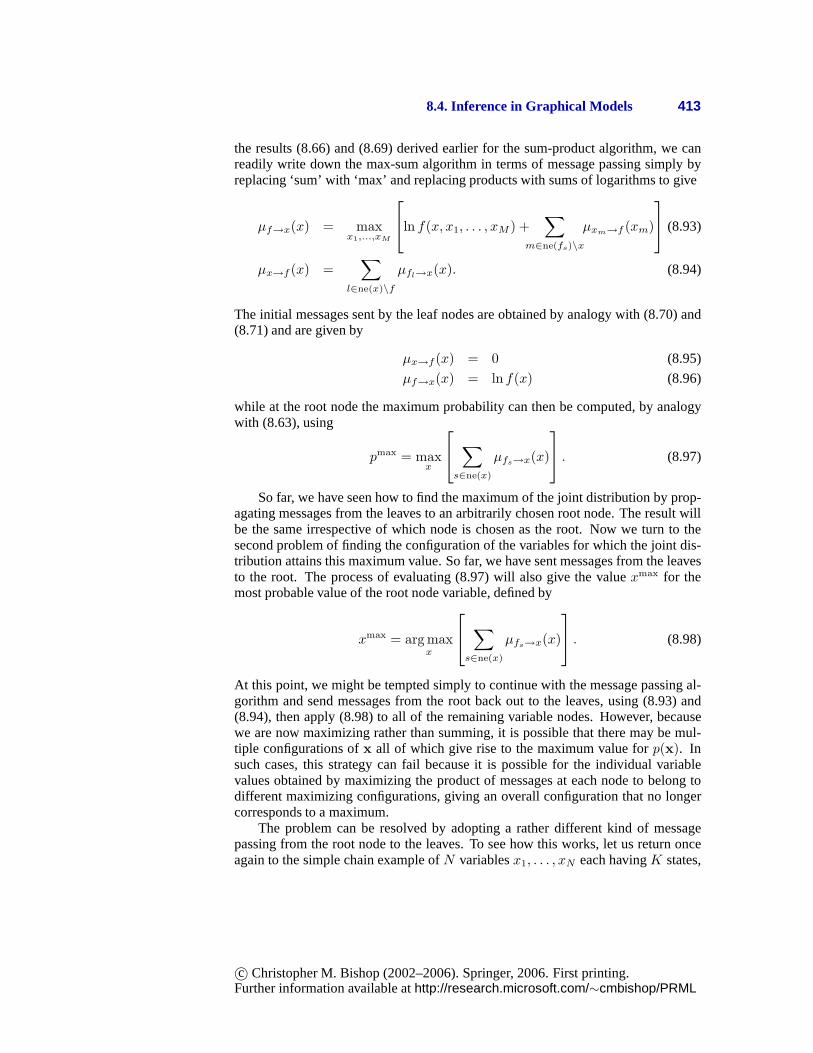
8.4. Inference in Graphical Models 413
the results (8.66) and (8.69) derived earlier for the sum-product algorithm, we canreadily write down the max-sum algorithm in terms of messagepassing simply byreplacing ‘sum’ with ‘max’ and replacing products with sumsof logarithms to give
µf→x(x) = maxx1,...,xM
ln f(x, x1, . . . , xM ) +
∑
m∈ne(fs)\x
µxm→f (xm)
(8.93)
µx→f (x) =∑
l∈ne(x)\f
µfl→x(x). (8.94)
The initial messages sent by the leaf nodes are obtained by analogy with (8.70) and(8.71) and are given by
µx→f(x) = 0 (8.95)
µf→x(x) = ln f(x) (8.96)
while at the root node the maximum probability can then be computed, by analogywith (8.63), using
pmax = maxx
∑
s∈ne(x)
µfs→x(x)
. (8.97)
So far, we have seen how to find the maximum of the joint distribution by prop-agating messages from the leaves to an arbitrarily chosen root node. The result willbe the same irrespective of which node is chosen as the root. Now we turn to thesecond problem of finding the configuration of the variables for which the joint dis-tribution attains this maximum value. So far, we have sent messages from the leavesto the root. The process of evaluating (8.97) will also give the valuexmax for themost probable value of the root node variable, defined by
xmax = arg maxx
∑
s∈ne(x)
µfs→x(x)
. (8.98)
At this point, we might be tempted simply to continue with themessage passing al-gorithm and send messages from the root back out to the leaves, using (8.93) and(8.94), then apply (8.98) to all of the remaining variable nodes. However, becausewe are now maximizing rather than summing, it is possible that there may be mul-tiple configurations ofx all of which give rise to the maximum value forp(x). Insuch cases, this strategy can fail because it is possible forthe individual variablevalues obtained by maximizing the product of messages at each node to belong todifferent maximizing configurations, giving an overall configuration that no longercorresponds to a maximum.
The problem can be resolved by adopting a rather different kind of messagepassing from the root node to the leaves. To see how this works, let us return onceagain to the simple chain example ofN variablesx1, . . . , xN each havingK states,
c© Christopher M. Bishop (2002–2006). Springer, 2006. First printing.Further information available athttp://research.microsoft.com/∼cmbishop/PRML
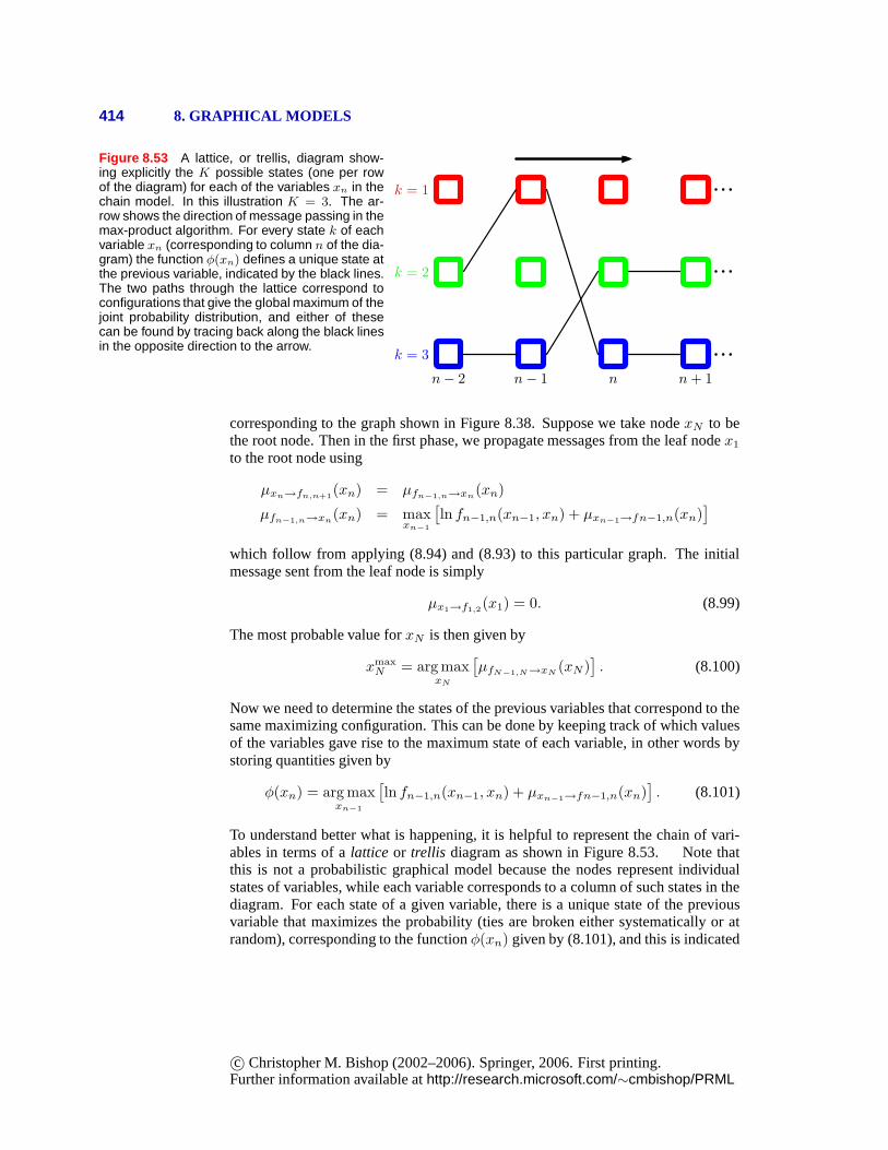
414 8. GRAPHICAL MODELS
Figure 8.53 A lattice, or trellis, diagram show-ing explicitly the K possible states (one per rowof the diagram) for each of the variables xn in thechain model. In this illustration K = 3. The ar-row shows the direction of message passing in themax-product algorithm. For every state k of eachvariable xn (corresponding to column n of the dia-gram) the function φ(xn) defines a unique state atthe previous variable, indicated by the black lines.The two paths through the lattice correspond toconfigurations that give the global maximum of thejoint probability distribution, and either of thesecan be found by tracing back along the black linesin the opposite direction to the arrow.
k = 1
k = 2
k = 3
n− 2 n− 1 n n+ 1
corresponding to the graph shown in Figure 8.38. Suppose we take nodexN to bethe root node. Then in the first phase, we propagate messages from the leaf nodex1
to the root node using
µxn→fn,n+1(xn) = µfn−1,n→xn
(xn)
µfn−1,n→xn(xn) = max
xn−1
[ln fn−1,n(xn−1, xn) + µxn−1→fn−1,n(xn)
]
which follow from applying (8.94) and (8.93) to this particular graph. The initialmessage sent from the leaf node is simply
µx1→f1,2(x1) = 0. (8.99)
The most probable value forxN is then given by
xmaxN = arg max
xN
[µfN−1,N→xN
(xN)]. (8.100)
Now we need to determine the states of the previous variablesthat correspond to thesame maximizing configuration. This can be done by keeping track of which valuesof the variables gave rise to the maximum state of each variable, in other words bystoring quantities given by
φ(xn) = arg maxxn−1
[ln fn−1,n(xn−1, xn) + µxn−1→fn−1,n(xn)
]. (8.101)
To understand better what is happening, it is helpful to represent the chain of vari-ables in terms of alattice or trellis diagram as shown in Figure 8.53. Note thatthis is not a probabilistic graphical model because the nodes represent individualstates of variables, while each variable corresponds to a column of such states in thediagram. For each state of a given variable, there is a uniquestate of the previousvariable that maximizes the probability (ties are broken either systematically or atrandom), corresponding to the functionφ(xn) given by (8.101), and this is indicated
c© Christopher M. Bishop (2002–2006). Springer, 2006. First printing.Further information available athttp://research.microsoft.com/∼cmbishop/PRML
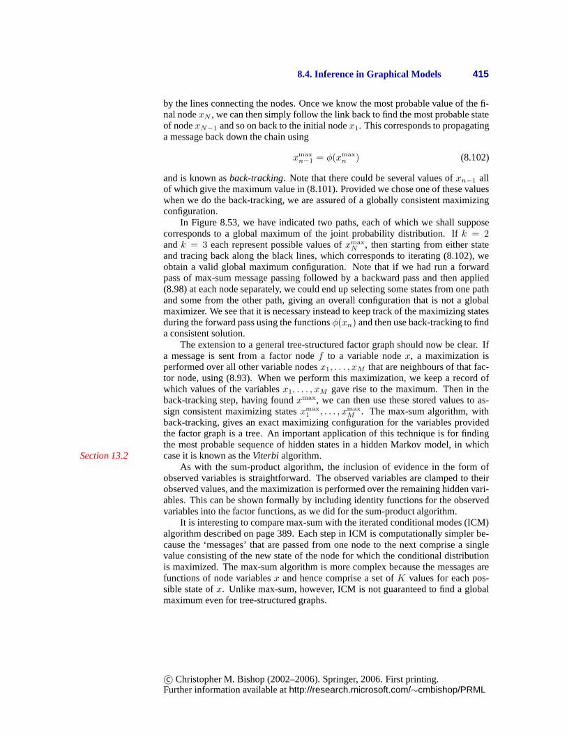
8.4. Inference in Graphical Models 415
by the lines connecting the nodes. Once we know the most probable value of the fi-nal nodexN , we can then simply follow the link back to find the most probable stateof nodexN−1 and so on back to the initial nodex1. This corresponds to propagatinga message back down the chain using
xmaxn−1 = φ(xmax
n ) (8.102)
and is known asback-tracking. Note that there could be several values ofxn−1 allof which give the maximum value in (8.101). Provided we choseone of these valueswhen we do the back-tracking, we are assured of a globally consistent maximizingconfiguration.
In Figure 8.53, we have indicated two paths, each of which we shall supposecorresponds to a global maximum of the joint probability distribution. If k = 2andk = 3 each represent possible values ofxmax
N , then starting from either stateand tracing back along the black lines, which corresponds toiterating (8.102), weobtain a valid global maximum configuration. Note that if we had run a forwardpass of max-sum message passing followed by a backward pass and then applied(8.98) at each node separately, we could end up selecting some states from one pathand some from the other path, giving an overall configurationthat is not a globalmaximizer. We see that it is necessary instead to keep track of the maximizing statesduring the forward pass using the functionsφ(xn) and then use back-tracking to finda consistent solution.
The extension to a general tree-structured factor graph should now be clear. Ifa message is sent from a factor nodef to a variable nodex, a maximization isperformed over all other variable nodesx1, . . . , xM that are neighbours of that fac-tor node, using (8.93). When we perform this maximization, we keep a record ofwhich values of the variablesx1, . . . , xM gave rise to the maximum. Then in theback-tracking step, having foundxmax, we can then use these stored values to as-sign consistent maximizing statesxmax
1 , . . . , xmaxM . The max-sum algorithm, with
back-tracking, gives an exact maximizing configuration forthe variables providedthe factor graph is a tree. An important application of this technique is for findingthe most probable sequence of hidden states in a hidden Markov model, in whichcase it is known as theViterbi algorithm.Section 13.2
As with the sum-product algorithm, the inclusion of evidence in the form ofobserved variables is straightforward. The observed variables are clamped to theirobserved values, and the maximization is performed over theremaining hidden vari-ables. This can be shown formally by including identity functions for the observedvariables into the factor functions, as we did for the sum-product algorithm.
It is interesting to compare max-sum with the iterated conditional modes (ICM)algorithm described on page 389. Each step in ICM is computationally simpler be-cause the ‘messages’ that are passed from one node to the nextcomprise a singlevalue consisting of the new state of the node for which the conditional distributionis maximized. The max-sum algorithm is more complex becausethe messages arefunctions of node variablesx and hence comprise a set ofK values for each pos-sible state ofx. Unlike max-sum, however, ICM is not guaranteed to find a globalmaximum even for tree-structured graphs.
c© Christopher M. Bishop (2002–2006). Springer, 2006. First printing.Further information available athttp://research.microsoft.com/∼cmbishop/PRML
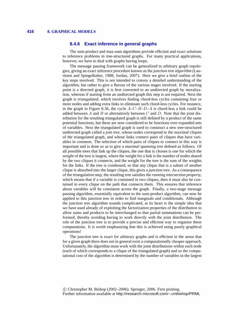
416 8. GRAPHICAL MODELS
8.4.6 Exact inference in general graphs
The sum-product and max-sum algorithms provide efficient and exact solutionsto inference problems in tree-structured graphs. For many practical applications,however, we have to deal with graphs having loops.
The message passing framework can be generalized to arbitrary graph topolo-gies, giving an exact inference procedure known as thejunction tree algorithm(Lau-ritzen and Spiegelhalter, 1988; Jordan, 2007). Here we givea brief outline of thekey steps involved. This is not intended to convey a detailedunderstanding of thealgorithm, but rather to give a flavour of the various stages involved. If the startingpoint is a directed graph, it is first converted to an undirected graph by moraliza-tion, whereas if starting from an undirected graph this stepis not required. Next thegraph istriangulated, which involves finding chord-less cycles containing four ormore nodes and adding extra links to eliminate such chord-less cycles. For instance,in the graph in Figure 8.36, the cycleA–C–B–D–A is chord-less a link could beadded betweenA andB or alternatively betweenC andD. Note that the joint dis-tribution for the resulting triangulated graph is still defined by a product of the samepotential functions, but these are now considered to be functions over expanded setsof variables. Next the triangulated graph is used to construct a new tree-structuredundirected graph called ajoin tree, whose nodes correspond to the maximal cliquesof the triangulated graph, and whose links connect pairs of cliques that have vari-ables in common. The selection of which pairs of cliques to connect in this way isimportant and is done so as to give amaximal spanning treedefined as follows. Ofall possible trees that link up the cliques, the one that is chosen is one for which theweightof the tree is largest, where the weight for a link is the number of nodes sharedby the two cliques it connects, and the weight for the tree is the sum of the weightsfor the links. If the tree is condensed, so that any clique that is a subset of anotherclique is absorbed into the larger clique, this gives ajunction tree. As a consequenceof the triangulation step, the resulting tree satisfies therunning intersection property,which means that if a variable is contained in two cliques, then it must also be con-tained in every clique on the path that connects them. This ensures that inferenceabout variables will be consistent across the graph. Finally, a two-stage messagepassing algorithm, essentially equivalent to the sum-product algorithm, can now beapplied to this junction tree in order to find marginals and conditionals. Althoughthe junction tree algorithm sounds complicated, at its heart is the simple idea thatwe have used already of exploiting the factorization properties of the distribution toallow sums and products to be interchanged so that partial summations can be per-formed, thereby avoiding having to work directly with the joint distribution. Therole of the junction tree is to provide a precise and efficientway to organize thesecomputations. It is worth emphasizing that this is achievedusing purely graphicaloperations!
The junction tree is exact for arbitrary graphs and is efficient in the sense thatfor a given graph there does not in general exist a computationally cheaper approach.Unfortunately, the algorithm must work with the joint distributions within each node(each of which corresponds to a clique of the triangulated graph) and so the compu-tational cost of the algorithm is determined by the number ofvariables in the largest
c© Christopher M. Bishop (2002–2006). Springer, 2006. First printing.Further information available athttp://research.microsoft.com/∼cmbishop/PRML
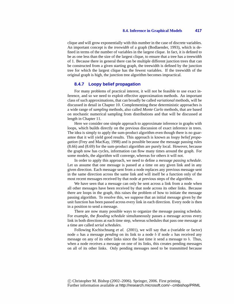
8.4. Inference in Graphical Models 417
clique and will grow exponentially with this number in the case of discrete variables.An important concept is thetreewidthof a graph (Bodlaender, 1993), which is de-fined in terms of the number of variables in the largest clique. In fact, it is defined tobe as one less than the size of the largest clique, to ensure that a tree has a treewidthof 1. Because there in general there can be multiple different junction trees that canbe constructed from a given starting graph, the treewidth isdefined by the junctiontree for which the largest clique has the fewest variables. If the treewidth of theoriginal graph is high, the junction tree algorithm becomesimpractical.
8.4.7 Loopy belief propagation
For many problems of practical interest, it will not be feasible to use exact in-ference, and so we need to exploit effective approximation methods. An importantclass of such approximations, that can broadly be calledvariationalmethods, will bediscussed in detail in Chapter 10. Complementing these deterministic approaches isa wide range ofsamplingmethods, also calledMonte Carlomethods, that are basedon stochastic numerical sampling from distributions and that will be discussed atlength in Chapter 11.
Here we consider one simple approach to approximate inference in graphs withloops, which builds directly on the previous discussion of exact inference in trees.The idea is simply to apply the sum-product algorithm even though there is no guar-antee that it will yield good results. This approach is knownasloopy belief propa-gation (Frey and MacKay, 1998) and is possible because the message passing rules(8.66) and (8.69) for the sum-product algorithm are purely local. However, becausethe graph now has cycles, information can flow many times around the graph. Forsome models, the algorithm will converge, whereas for others it will not.
In order to apply this approach, we need to define amessage passing schedule.Let us assume that one message is passed at a time on any given link and in anygiven direction. Each message sent from a node replaces any previous message sentin the same direction across the same link and will itself be afunction only of themost recent messages received by that node at previous stepsof the algorithm.
We have seen that a message can only be sent across a link from anode whenall other messages have been received by that node across itsother links. Becausethere are loops in the graph, this raises the problem of how toinitiate the messagepassing algorithm. To resolve this, we suppose that an initial message given by theunit function has been passed across every link in each direction. Every node is thenin a position to send a message.
There are now many possible ways to organize the message passing schedule.For example, theflooding schedulesimultaneously passes a message across everylink in both directions at each time step, whereas schedulesthat pass one message ata time are calledserial schedules.
Following Kschischnanget al. (2001), we will say that a (variable or factor)nodea has a messagependingon its link to a nodeb if node a has received anymessage on any of its other links since the last time it send a message tob. Thus,when a node receives a message on one of its links, this creates pending messageson all of its other links. Only pending messages need to be transmitted because
c© Christopher M. Bishop (2002–2006). Springer, 2006. First printing.Further information available athttp://research.microsoft.com/∼cmbishop/PRML
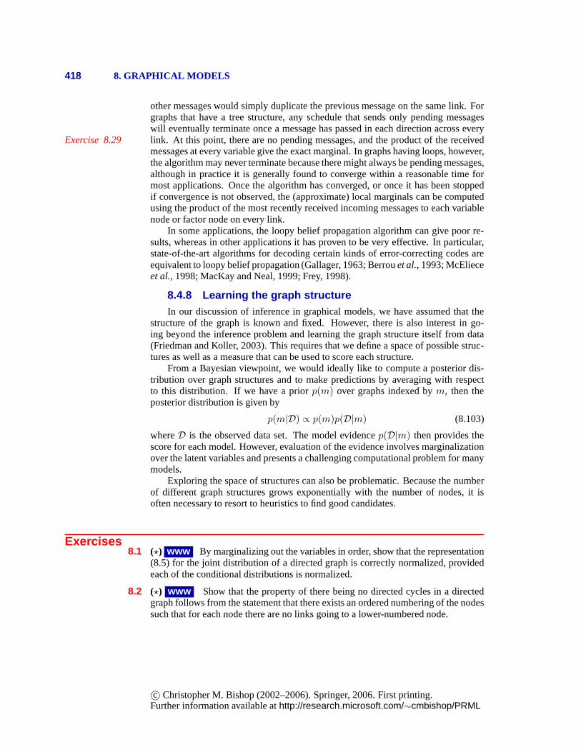
418 8. GRAPHICAL MODELS
other messages would simply duplicate the previous messageon the same link. Forgraphs that have a tree structure, any schedule that sends only pending messageswill eventually terminate once a message has passed in each direction across everylink. At this point, there are no pending messages, and the product of the receivedExercise 8.29messages at every variable give the exact marginal. In graphs having loops, however,the algorithm may never terminate because there might always be pending messages,although in practice it is generally found to converge within a reasonable time formost applications. Once the algorithm has converged, or once it has been stoppedif convergence is not observed, the (approximate) local marginals can be computedusing the product of the most recently received incoming messages to each variablenode or factor node on every link.
In some applications, the loopy belief propagation algorithm can give poor re-sults, whereas in other applications it has proven to be veryeffective. In particular,state-of-the-art algorithms for decoding certain kinds oferror-correcting codes areequivalent to loopy belief propagation (Gallager, 1963; Berrouet al., 1993; McElieceet al., 1998; MacKay and Neal, 1999; Frey, 1998).
8.4.8 Learning the graph structureIn our discussion of inference in graphical models, we have assumed that the
structure of the graph is known and fixed. However, there is also interest in go-ing beyond the inference problem and learning the graph structure itself from data(Friedman and Koller, 2003). This requires that we define a space of possible struc-tures as well as a measure that can be used to score each structure.
From a Bayesian viewpoint, we would ideally like to compute aposterior dis-tribution over graph structures and to make predictions by averaging with respectto this distribution. If we have a priorp(m) over graphs indexed bym, then theposterior distribution is given by
p(m|D) ∝ p(m)p(D|m) (8.103)
whereD is the observed data set. The model evidencep(D|m) then provides thescore for each model. However, evaluation of the evidence involves marginalizationover the latent variables and presents a challenging computational problem for manymodels.
Exploring the space of structures can also be problematic. Because the numberof different graph structures grows exponentially with thenumber of nodes, it isoften necessary to resort to heuristics to find good candidates.
Exercises8.1 (?) www By marginalizing out the variables in order, show that the representation
(8.5) for the joint distribution of a directed graph is correctly normalized, providedeach of the conditional distributions is normalized.
8.2 (?) www Show that the property of there being no directed cycles in a directedgraph follows from the statement that there exists an ordered numbering of the nodessuch that for each node there are no links going to a lower-numbered node.
c© Christopher M. Bishop (2002–2006). Springer, 2006. First printing.Further information available athttp://research.microsoft.com/∼cmbishop/PRML
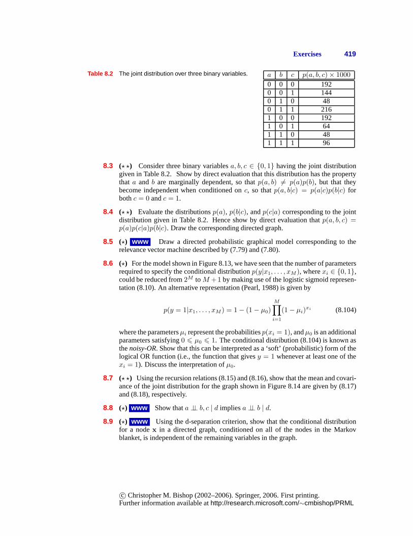
Exercises 419
Table 8.2 The joint distribution over three binary variables. a b c p(a, b, c) × 1000
0 0 0 1920 0 1 1440 1 0 480 1 1 2161 0 0 1921 0 1 641 1 0 481 1 1 96
8.3 (? ?) Consider three binary variablesa, b, c ∈ {0, 1} having the joint distributiongiven in Table 8.2. Show by direct evaluation that this distribution has the propertythat a and b are marginally dependent, so thatp(a, b) 6= p(a)p(b), but that theybecome independent when conditioned onc, so thatp(a, b|c) = p(a|c)p(b|c) forbothc = 0 andc = 1.
8.4 (? ?) Evaluate the distributionsp(a), p(b|c), andp(c|a) corresponding to the jointdistribution given in Table 8.2. Hence show by direct evaluation thatp(a, b, c) =p(a)p(c|a)p(b|c). Draw the corresponding directed graph.
8.5 (?) www Draw a directed probabilistic graphical model corresponding to therelevance vector machine described by (7.79) and (7.80).
8.6 (?) For the model shown in Figure 8.13, we have seen that the number of parametersrequired to specify the conditional distributionp(y|x1, . . . , xM ), wherexi ∈ {0, 1},could be reduced from2M toM +1 by making use of the logistic sigmoid represen-tation (8.10). An alternative representation (Pearl, 1988) is given by
p(y = 1|x1, . . . , xM ) = 1 − (1 − µ0)
M∏
i=1
(1 − µi)xi (8.104)
where the parametersµi represent the probabilitiesp(xi = 1), andµ0 is an additionalparameters satisfying0 6 µ0 6 1. The conditional distribution (8.104) is known asthenoisy-OR. Show that this can be interpreted as a ‘soft’ (probabilistic) form of thelogical OR function (i.e., the function that givesy = 1 whenever at least one of thexi = 1). Discuss the interpretation ofµ0.
8.7 (? ?) Using the recursion relations (8.15) and (8.16), show that the mean and covari-ance of the joint distribution for the graph shown in Figure 8.14 are given by (8.17)and (8.18), respectively.
8.8 (?) www Show thata ⊥⊥ b, c | d impliesa ⊥⊥ b | d.
8.9 (?) www Using the d-separation criterion, show that the conditional distributionfor a nodex in a directed graph, conditioned on all of the nodes in the Markovblanket, is independent of the remaining variables in the graph.
c© Christopher M. Bishop (2002–2006). Springer, 2006. First printing.Further information available athttp://research.microsoft.com/∼cmbishop/PRML
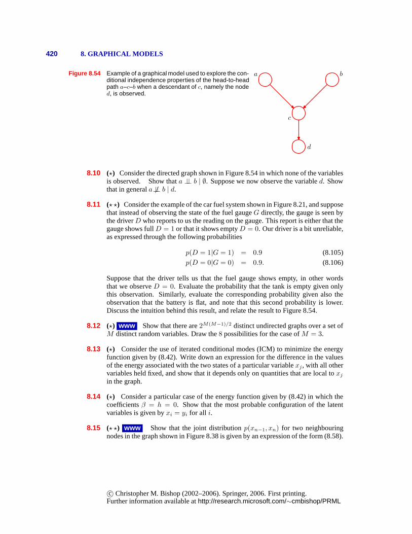
420 8. GRAPHICAL MODELS
Figure 8.54 Example of a graphical model used to explore the con-ditional independence properties of the head-to-headpath a–c–b when a descendant of c, namely the noded, is observed.
c
a b
d
8.10 (?) Consider the directed graph shown in Figure 8.54 in which none of the variablesis observed. Show thata ⊥⊥ b | ∅. Suppose we now observe the variabled. Showthat in generala 6⊥⊥ b | d.
8.11 (? ?) Consider the example of the car fuel system shown in Figure 8.21, and supposethat instead of observing the state of the fuel gaugeG directly, the gauge is seen bythe driverD who reports to us the reading on the gauge. This report is either that thegauge shows fullD = 1 or that it shows emptyD = 0. Our driver is a bit unreliable,as expressed through the following probabilities
p(D = 1|G = 1) = 0.9 (8.105)
p(D = 0|G = 0) = 0.9. (8.106)
Suppose that the driver tells us that the fuel gauge shows empty, in other wordsthat we observeD = 0. Evaluate the probability that the tank is empty given onlythis observation. Similarly, evaluate the corresponding probability given also theobservation that the battery is flat, and note that this second probability is lower.Discuss the intuition behind this result, and relate the result to Figure 8.54.
8.12 (?) www Show that there are2M(M−1)/2 distinct undirected graphs over a set ofM distinct random variables. Draw the8 possibilities for the case ofM = 3.
8.13 (?) Consider the use of iterated conditional modes (ICM) to minimize the energyfunction given by (8.42). Write down an expression for the difference in the valuesof the energy associated with the two states of a particular variablexj, with all othervariables held fixed, and show that it depends only on quantities that are local toxj
in the graph.
8.14 (?) Consider a particular case of the energy function given by (8.42) in which thecoefficientsβ = h = 0. Show that the most probable configuration of the latentvariables is given byxi = yi for all i.
8.15 (? ?) www Show that the joint distributionp(xn−1, xn) for two neighbouringnodes in the graph shown in Figure 8.38 is given by an expression of the form (8.58).
c© Christopher M. Bishop (2002–2006). Springer, 2006. First printing.Further information available athttp://research.microsoft.com/∼cmbishop/PRML
Exercises 421
8.16 (? ?) Consider the inference problem of evaluatingp(xn|xN ) for the graph shownin Figure 8.38, for all nodesn ∈ {1, . . . , N − 1}. Show that the message passingalgorithm discussed in Section 8.4.1 can be used to solve this efficiently, and discusswhich messages are modified and in what way.
8.17 (? ?) Consider a graph of the form shown in Figure 8.38 havingN = 5 nodes, inwhich nodesx3 andx5 are observed. Use d-separation to show thatx2 ⊥⊥ x5 | x3.Show that if the message passing algorithm of Section 8.4.1 is applied to the evalu-ation ofp(x2|x3, x5), the result will be independent of the value ofx5.
8.18 (? ?) www Show that a distribution represented by a directed tree can triviallybe written as an equivalent distribution over the corresponding undirected tree. Alsoshow that a distribution expressed as an undirected tree can, by suitable normaliza-tion of the clique potentials, be written as a directed tree.Calculate the number ofdistinct directed trees that can be constructed from a givenundirected tree.
8.19 (? ?) Apply the sum-product algorithm derived in Section 8.4.4 tothe chain-of-nodes model discussed in Section 8.4.1 and show that the results (8.54), (8.55), and(8.57) are recovered as a special case.
8.20 (?) www Consider the message passing protocol for the sum-product algorithm ona tree-structured factor graph in which messages are first propagated from the leavesto an arbitrarily chosen root node and then from the root nodeout to the leaves. Useproof by induction to show that the messages can be passed in such an order thatat every step, each node that must send a message has receivedall of the incomingmessages necessary to construct its outgoing messages.
8.21 (? ?) www Show that the marginal distributionsp(xs) over the sets of variablesxs associated with each of the factorsfx(xs) in a factor graph can be found by firstrunning the sum-product message passing algorithm and thenevaluating the requiredmarginals using (8.72).
8.22 (?) Consider a tree-structured factor graph, in which a given subset of the variablenodes form a connected subgraph (i.e., any variable node of the subset is connectedto at least one of the other variable nodes via a single factornode). Show how thesum-product algorithm can be used to compute the marginal distribution over thatsubset.
8.23 (? ?) www In Section 8.4.4, we showed that the marginal distributionp(xi) for avariable nodexi in a factor graph is given by the product of the messages arriving atthis node from neighbouring factor nodes in the form (8.63).Show that the marginalp(xi) can also be written as the product of the incoming message along any one ofthe links with the outgoing message along the same link.
8.24 (? ?) Show that the marginal distribution for the variablesxs in a factorfs(xs) ina tree-structured factor graph, after running the sum-product message passing algo-rithm, can be written as the product of the message arriving at the factor node alongall its links, times the local factorf(xs), in the form (8.72).
c© Christopher M. Bishop (2002–2006). Springer, 2006. First printing.Further information available athttp://research.microsoft.com/∼cmbishop/PRML
422 8. GRAPHICAL MODELS
8.25 (? ?) In (8.86), we verified that the sum-product algorithm run on the graph inFigure 8.51 with nodex3 designated as the root node gives the correct marginal forx2. Show that the correct marginals are obtained also forx1 andx3. Similarly, showthat the use of the result (8.72) after running the sum-product algorithm on this graphgives the correct joint distribution forx1, x2.
8.26 (?) Consider a tree-structured factor graph over discrete variables, and suppose wewish to evaluate the joint distributionp(xa, xb) associated with two variablesxa andxb that do not belong to a common factor. Define a procedure for using the sum-product algorithm to evaluate this joint distribution in which one of the variables issuccessively clamped to each of its allowed values.
8.27 (? ?) Consider two discrete variablesx andy each having three possible states, forexamplex, y ∈ {0, 1, 2}. Construct a joint distributionp(x, y) over these variableshaving the property that the valuex that maximizes the marginalp(x), along withthe valuey that maximizes the marginalp(y), together have probability zero underthe joint distribution, so thatp(x, y) = 0.
8.28 (? ?) www The concept of apendingmessage in the sum-product algorithm fora factor graph was defined in Section 8.4.7. Show that if the graph has one or morecycles, there will always be at least one pending message irrespective of how longthe algorithm runs.
8.29 (? ?) www Show that if the sum-product algorithm is run on a factor graph with atree structure (no loops), then after a finite number of messages have been sent, therewill be no pending messages.
c© Christopher M. Bishop (2002–2006). Springer, 2006. First printing.Further information available athttp://research.microsoft.com/∼cmbishop/PRML