Pattern Selection and the Direction of Stripes in Two ... · Here we assume that d is larger than 1, and hence diffusivity of v is larger than that of u. Now we consider the equilibrium

3

Review __________________________________________________________________ Forma, 18, 3–18, 2003

Pattern Selection and the Direction of Stripes in Two-DimensionalTuring Systems for Skin Pattern Formation of Fishes

Hiroto SHOJI* and Yoh IWASA

Department of Biology, Faculty of Sciences, Kyushu University, Fukuoka 812-8581, Japan*E-mail address: [email protected]

(Received November 29, 2002; Accepted December 25, 2002)

Keywords: Reaction-Diffusion System, Turing, Pattern Selection, Anistropic Diffusion,Directionality of Stripes

Abstract. Turing mechanism explains the pattern formation in a uniform field in whichtwo substances (e.g. activator and inhibitor) interact locally and diffuse randomly. Two-dimensional Turing models can generate stationary spatial patterns either with stripes orwith spots, and have been adopted to explain the skin pattern formation of animals. Wefirst discuss the effect of the choice of reaction terms on pattern selection, whether spotsor stripes are formed. It is shown that the relative distance of the equilibrium level ofactivator between the upper and lower limitations has a very strong effect on the patternselection. Secondly, we focus on the direction of the stripes generated by Turing modelwith anisotropic diffusion in order to explain the directionality of stripes on fish skin inclosely related species. Relative magnitude of anisotropy of the two substances is shownto determine whether stripes are vertical or horizontal.

1. Introduction

Some animals have striped pattern on their skin, exemplified by zebra or tiger’scoating. The developmental pattern formation of animal coating has been studiedmathematically by Turing system (MEINHARDT, 1982; MURRAY, 1989). It is a pair ofpartial differential equations, and represents the time development of reacting and diffusingchemicals, which can evolve spontaneously to spatially heterogeneous stationary patternfrom an initially uniform distribution (TURING, 1952). TURING (1952) specifically considereda system of two chemicals, an activator and an inhibitor, where the activator enhances itsown production rate and also promotes the production of the inhibitor whilst the inhibitorsuppresses both activator and inhibitor. The diffusion coefficient of the inhibitor is muchlarger than that of the activator. Without diffusion, the local reaction of the two substancesis stable and converges to the equilibrium. However, with diffusion, the uniform distributionsof both substances with concentrations at the equilibrium are unstable, and a spatiallyheterogeneous pattern emerges spontaneously, called Turing instability. This simplemechanism suggests that reaction of a small number of chemicals and their randomdiffusion can create stable non-uniform patterns in a perfectly homogeneous field.

4 H. SHOJI and Y. IWASA

MEINHARDT (1982) discussed many cases of pattern formation in development that arelikely to be explained by reaction-diffusion model, including regeneration and patternformation of hydras (MEINHARDT, 1982). MURRAY (1989) also explained various phenomenaof biological pattern formation including the patterns of animal coating. Although patternsof mammal coating are quite suggestive of the involvement of Turing mechanism, theirpattern is formed in early developmental stages, and the number of stripes does not changein their lifetime even if the body size grows considerably. In contrast, the stripe pattern onfish skin changes as the fish body size increases (KONDO and ASAI, 1995). The number ofstripes increases with the body size but the width of each stripe and their distance betweenstripes remain almost unchanged. KONDO and ASAI (1995) studied the skin patterns ofseveral species of tropical fishes, and showed that the change of their skin patterns can beexplained very accurately by a simple reaction-diffusion model of Turing type.

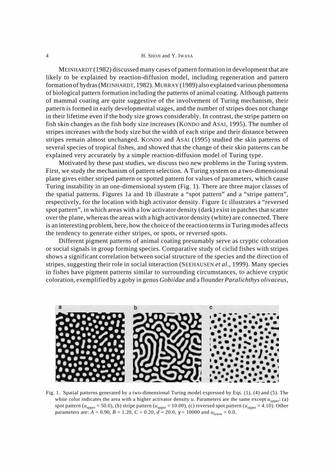
Motivated by these past studies, we discuss two new problems in the Turing system.First, we study the mechanism of pattern selection. A Turing system on a two-dimensionalplane gives either striped pattern or spotted pattern for values of parameters, which causeTuring instability in an one-dimensional system (Fig. 1). There are three major classes ofthe spatial patterns. Figures 1a and 1b illustrate a “spot pattern” and a “stripe pattern”,respectively, for the location with high activator density. Figure 1c illustrates a “reversedspot pattern”, in which areas with a low activator density (dark) exist in patches that scatterover the plane, whereas the areas with a high activator density (white) are connected. Thereis an interesting problem, here, how the choice of the reaction terms in Turing modes affectsthe tendency to generate either stripes, or spots, or reversed spots.

Different pigment patterns of animal coating presumably serve as cryptic colorationor social signals in group forming species. Comparative study of ciclid fishes with stripesshows a significant correlation between social structure of the species and the direction ofstripes, suggesting their role in social interaction (SEEHAUSEN et al., 1999). Many speciesin fishes have pigment patterns similar to surrounding circumstances, to achieve crypticcoloration, exemplified by a goby in genus Gobiidae and a flounder Paralichthys olivaceus,

Fig. 1. Spatial patterns generated by a two-dimensional Turing model expressed by Eqs. (1), (4) and (5). Thewhite color indicates the area with a higher activator density u. Parameters are the same except uupper: (a)spot pattern (uupper = 50.0), (b) stripe pattern (uupper = 10.00), (c) reversed spot pattern (uupper = 4.10). Otherparameters are: A = 0.90, B = 1.20, C = 0.20, d = 20.0, γ = 10000 and ulower = 0.0.

Pattern Selection and the Direction of Stripes in Two-Dimensional Turing Systems 5

suggesting that the pattern might serve as a means of predator avoidance (KUWAMURA andKARINO, 1999). Within the same species of fish Hypostomus plecostomus, some subspecieshas spot pattern and others has stripes (YAMAGUCHI, 2002).

Secondly, the directionality of stripes formed in Turing systems provides an interestingproblem. Since fish have scales, fish skin is morphologically different along the AP axisand along the dorso-ventral (DV) axis. Therefore it is plausible to assume that the diffusioncoefficient is different between directions. We study the reaction-diffusion model wherethe substances can diffuse faster in a certain specific direction than in a directionperpendicular to it. Hence the diffusion of the two substances can be anisotropic. Resultsof numerical analysis in this work explain many features of pattern formation shown byseveral species in genus Genicanthus.

We also develop a heuristic argument of the direction of stripes in more generalsituations in which the diffusive direction may differ between the two substances. As aresult we have derived a formula for the direction of stripes, based on the most unstablemode of deviation from the uniform steady state.

2. Turing System

TURING (1952) showed that two diffusive chemicals that react each other can generatespatially heterogeneous patterns spontaneously from a uniform initial distribution. Ingeneral, the model can be written as follows,

∂∂

= ∇ + ( ) ∂∂

= ∇ + ( ) ( )u

tu f u v

v

td v g u v2 2 1γ γ, , , ,and

where u and v are the concentrations of two substances which differ in diffusivity. Byrescaling the space variable, we made the diffusion coefficient of u equal to 1. On the otherhand, two reaction terms are multiplied by a common factor γ, and the diffusion coefficientfor v is replaced by the ratio of diffusion coefficient of the two substances, denoted by d.Here we assume that d is larger than 1, and hence diffusivity of v is larger than that of u.

Now we consider the equilibrium (u0, v0) of ordinary differential equationscorresponding to partial differential Eq. (1). It satisfies: f(u0, v0) = 0, and g(u0, v0) = 0. Thisis linearly stable in the ordinary differential equation:

∂∂

+ ∂∂

< ∂∂

∂∂

− ∂∂

∂∂

> ( )f

u

g

v

f

u

g

v

f

v

g

u0 0 2, ,and

where all the partial derivatives are evaluated at equilibrium (u0, v0). Second, we considerthe local stability of the uniform steady state u = u0 and v = v0. This steady state solutionis unstable in the partial differential equations given by Eq. (1). This leads to:

df

u

g

vd

f

u

g

vd

f

u

g

v

f

v

g

u

∂∂

+ ∂∂

> ∂∂

+ ∂∂

− ∂∂

∂∂

− ∂∂

∂∂

> ( )0 4 0 32

, .and


The model satisfying Eqs. (2) and (3) is called a Turing system, and the parameter regionfor a given model to be a Turing system is called Turing space (MURRAY, 1989).

SHOJI et al. (2003b) examined the dimensionless reaction diffusion system as Eq. (1)with the linear reaction terms (following KONDO and ASAI, 1995; ASAI et al., 1999):

f u v Au v C g u v Bu v, , , ,( ) = − + ( ) = − − ( )and 1 4

where A, B and C are constants.In the numerical calculation of Eqs. (1) and (4), the deviation of two variables from

the equilibrium increases with time and diverges to positive and negative infinity. For themodel to have a stable stationary distribution of finite magnitude, we need to add terms toconstrain the variables within a finite range.

3. Pattern Selection Problem—Spot, Stripe, or Reversed Spot

We studied how the choice of the reaction terms in Turing modes affects the tendencyto generate either stripes, or spots, or reversed spots. We focus on the role of non-linearityin reaction terms that constrain the variables within a fixed range.

3.1. Periodic pattern in one dimensionalBefore examining the pattern selection of two-dimensional models, we first consider

the condition in which stable periodic pattern can be formed in a one-dimensional Turingmodel with linear reaction terms and constraints. We can show that linear models cangenerate stable periodic patterns if both variables are constrained from above and frombelow (e.g. KONDO and ASAI, 1995). To be specific, we introduced the constraint of u, asfollows:

u u ulower upper≤ ≤ ( ), 5

where ulower and uupper are constants. We call these as lower and upper limitations,respectively. We may also introduce a similar constraint with respect to v. There are fourpossible ways of constraint: the upper limitation of u, the lower limitation of u; the lowerupper limitation of v; and the lower limitation of v. We studied all the possible combinationsof these four ways of introducing constraints. The result is very clear—the activator, butnot the inhibitor, must be constrained both from above and from below for the model togenerate a stable periodic pattern in one-dimensional model, given by Eqs. (1) and (4),provided that parameters are within the Turing space. See SHOJI et al. (2003b) for detail.

3.2. Stripe, spots and reversed spots generated by linear systemWe then discuss two-dimensional patterns generated by linear model given by Eqs. (1)

and (4) with constraint Eq. (5). We have done all the simulation in this chapter by the sameanalysis explained below. We chose parameter and parameter range of reaction term as: γ= 10000, d = 20.0, C = 0.20, 0.0 ≤ A ≤ 1.2 and 0.0 ≤ B ≤ 6.0. Most of these parameters arein the Turing Space (see Fig. 2). The simulations were performed with periodic boundary


condition in a square domain of size: 2.0 × 2.0 (grid: 200 × 200). A simple explicit schemeis adopted. To satisfy the stability condition for numerical analysis, mesh size was chosento be 1.0 × 10–6. The fixed parameter was γ = 10000. We tested three initial conditionswhere value of u and v are equilibrium values added by small random deviations. The timeat which we stopped calculation was sufficiently long, and we can safely regard that thepattern would no longer change from the one obtained in the end of simulation even if weincrease the calculation time further.

We examine the effect of the constraint in determining pattern selection in the two-dimensional model. First, we note that, because of linear kinetics adopted here, the propertyof the model should not be changed by rescaling variables and time or space parameters.Hence whether the model generates patterns with spots, stripes or reversed spots should beunchanged if |umax – ueq| and |ueq – umin| are multiplied by the same factor, and hence onlythe ratio of |umax – ueq| to |ueq – umin| affects the pattern selection. We here focus on thepatterns generated by each parameter of Eqs. (1) and (4) with constraint Eq. (5). Due to thelinear nature of the kinetics, shifting of variables also should not affect the patternselection, indicating that the results is independent of parameter C in Eq. (4).

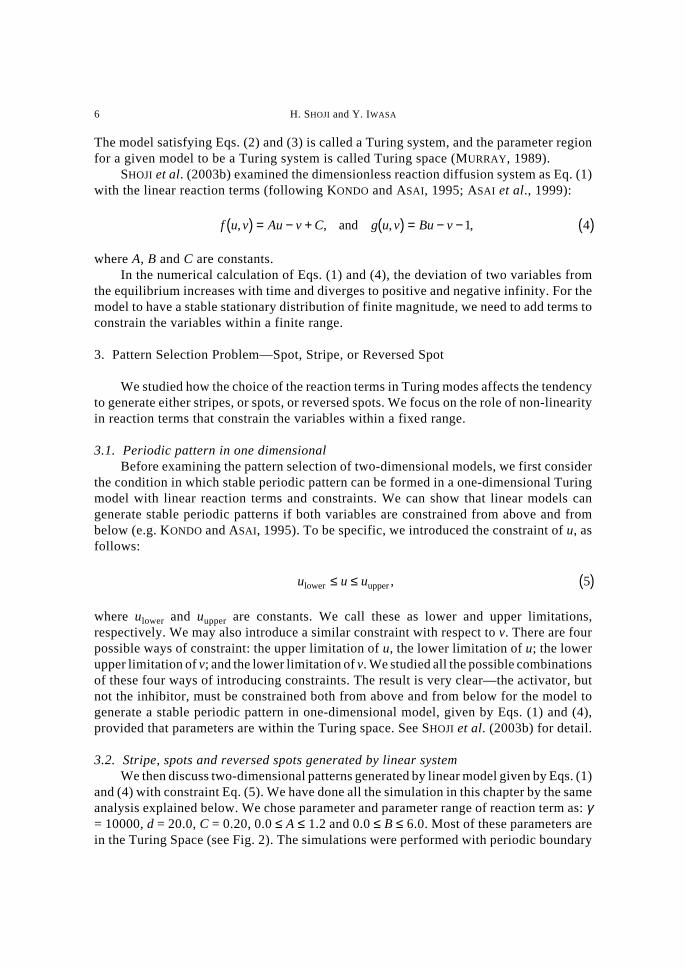
In Fig. 2, we have different cases of the ratio of |umax – ueq| and |ueq – umin|. Differentsymbols indicate the produced patterns. We judged each pattern to be one of the three byeye. Two axes are A and B. Figure 2a shows the results when the distance between theequilibrium value of u and upper limitation is five times as large as the distance betweenequilibrium u and lower limitation (|umax – ueq| = 5|ueq – umin|). For almost all parameters

Fig. 2. The parameter regions in which stripes, spots, and reversed spots were generated. Dynamics expressedby Eqs. (1) and (4) were adopted. The upper and lower limitations were realized by resetting the variableswhenever they go outside of the allowed interval. � with box: reversed spot, �: stripe pattern, �: spotpattern, ×: homogeneous pattern. The area surrounded by four broken lines is the Turing space derived fromEqs. (2) and (3). Other parameters are fixed as: C = 0.20, d = 20.0 and γ = 10000. (a) The distance from theequilibrium point to the upper limitation is 5.0 and one to lower limitation is 1.0. Spots pattern are producedin most of the Turing space. (b) The distance from the equilibrium point to upper limitation and the one tothe lower limitation are both 1.0. The stripe patterns were produced in most of the Turing space. (c) Thedistance from the equilibrium point to upper limitation is 1.0 and one to lower limitation is 5.0. The reversedspots pattern were produced in the large part of the Turing space.


in the Turing space (see Fig. 2), the model generated spot patterns in which white spots ofhigh u are evenly scattered and the black areas are connected with each other. Figure 2bshows the results when the distance between the equilibrium value of u and upper limitationis equal to the distance between the equilibrium and lower limitation (|umax – ueq| = |ueq –umin|). The stripe patterns appeared in almost all area of Turing space, in spite that stripedpatterns are considered rather difficult to generate by reaction diffusion models (MURRAY,1989). Figure 2c shows the results when the distance between equilibrium value of u andupper limitation is five times small as the distance between equilibrium point of u and lowerlimitation (5|umax – ueq| = |ueq – umin|). Figure 2c shows the distribution of the generatedpatterns at each parameter in Eqs. (1) and (4) with constraint Eq. (5). Now, the reversed spotpatterns, which are very hard to produce by many nonlinear models, appeared in almost allarea of Turing space.

Comparison of three cases in Fig. 2 suggests that the relative position of theequilibrium u between upper limitation and lower limitation plays a critical role indetermining the pattern to form. If the difference between equilibrium u to upper limitationand that between equilibrium and lower limitation are similar, the stripe patterns willemerge. If the difference between equilibrium u and upper limitation is larger than thedifference between the equilibrium and lower limitation, spot patterns will emerge. Incontrast, the difference between equilibrium u and lower limitation is larger than that toupper limitation, the reversed spot patterns will emerge. The result is independent of theabsolute size of the constrain interval, but only depends on the relative position of theequilibrium between upper and lower limitations. We also examined the effect of d, themagnitude of diffusion coefficient of inhibitor relative to that of the activator. The size ofthe Turing space changed with d, but the patterns generated by the model in the Turingspace was independent of d. See SHOJI et al. (2003b) for details.

3.3. Pattern selection of nonlinear reaction termsTo relate the conclusion of the constrained linear kinetics with the behavior of general

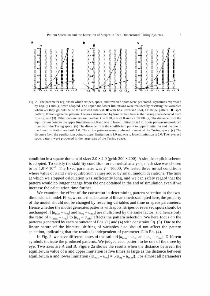
nonlinear models, we noted the shape of null-clines of the ordinary differential equations.Lower and upper limitations of activator level u to be Eq. (5) can be realized by anadditional term in the right hand side of Eq. (1) which are very small within the interval butbecomes very large near the points of limitation. For example a lower limitation “u ≥ umin”can be realized by a factor that is very small in magnitude for u > umin, but becomes apositive term with a very large magnitude near u ≈ umin. An upper limitation of u ≤ umax canbe realized by a term that is very small in magnitude for u < umax but becomes clearlynegative with a large magnitude near u ≈ umax. We can produce such a constraint byadditional terms, (umin/u)10 – (u/umax)10, in du/dt in Eq. (4). Figure 3 illustrates the null-clines of the linear reaction term (Fig. 3a), and linear terms with additional constrain termsas discussed above (Fig. 3b).

If we draw null-cline for u, f(u, v) = 0 for the model with additional terms for constraint,it has a sharp increase near the lower limitation (u ≈ umin) and a sharp decline near the upperlimitation (u ≈ umax). This is illustrated clearly by the contrast between Fig. 3b (withconstraint) and Fig. 3a (without constraint). Hence the constraint modifies the shape ofnull-cline f(u, v) = 0. Conversely, if a null-cline of a given non-linear model increasessharply at a low level or if the null-cline decreases sharply at a high level, we can guess that


the reaction terms in fact have a property working effectively as the lower and upperlimitations.

The nonlinear dynamics proposed previously for Turing mechanisms may have null-clines similar to the ones with linear dynamics with additional terms for constraint. We maydiscuss their similarity and difference by examining their null-clines: f(u, v) = 0 and g(u,v) = 0. Combining this with the result of linear kinetics with constraint—the relativelocation of equilibrium to the lower or to the upper limit of the model can make spot, stripeor reversed stripe. In SHOJI et al. (2003b), we examined the shape of null-clines of non-linear Turing models and discussed insights obtained on their behavior of pattern selectionfrom the result of linear kinetics and constraint.

3.4. Frequency distribution of activator levelThe effect of constraints to the spatial patterns generated by the model can be

understood more intuitively by examining the distribution of activator level.The distribution of sampled values of activator level u for a stripe pattern are of M-

shape with two peaks in the highest and the lowest value and with rather low level in theintermediate value. In contrast, the distribution of sampled u value for a spot pattern isshifted toward left and a tail toward right. In contrast, the distribution of u for a reversedspot pattern has a peak toward right. We generated the distribution of activator level u forspatial patterns generated by linear and nonlinear models with or without additionalconstraints, with many different parameter values. However we always have a clearcorrespondence of the spatial pattern (spot, stripe, or reversed stripe) and the shape ofdistributions (see SHOJI et al. (2003b) for detail).

Fig. 3. The null-clines. (a) Linear kinetics given by Eq. (4). (b) The null clines of a modified model with linearreaction terms of Eq. (4) with additional constraint terms, (umin/u)10 – (u/umax)10.


We can quantify the difference between these by a third moment of the distribution ofactivator level u. According to the simulations with different reaction terms and differentparameters, the average of u is almost always very close to the equilibrium value. When thedistribution are lean to leftward, the third moment is positive, and when the distribution arelean to rightward, it is negative. We can clearly classify the patterns by using the thirdmoment. When the third moment is clearly positive, the patterns are of spot patterns. Whenthe third moment are nearly equal 0, the patterns are stripe patterns. When the third momentare clearly negative, the patterns are reversed spot patterns. This result holds for differentchoice of reaction terms and parameters.

Based on this result, the effect of constraints from above or from below can beunderstood intuitively. A two-dimensional Turing pattern determines the relative positionof the equilibrium point between upper and lower limitations. If the limitation from belowis closer to the equilibrium than the limitation from the above, and if the mean is close tothe equilibrium value, this would produce a positive third moment of the distribution of u.Hence this explains why spot patterns are generated (white spots are scattered over blackregion). In contrast if the limitation from above is closer to the equilibrium than that fromthe below, a negative third moment of the distribution of u is created, resulting in reversedspot patterns (with black spots scattered over white regions). If the distance between thelimitation from above to the equilibrium and that between the limitation from below to theequilibrium is similar in magnitude, we have a distribution of activator level u with the thirdmoment close to zero, resulting in patterns with stripes.

DILLON et al. (1994) analyzed pattern formation of Turing system with severaldifferent boundary conditions (i.e. Neumann boundary condition, Dirichlet boundarycondition, and the boundary condition of the mixture of these two) for one-dimensionalmodel. MURRAY (1989) also studied the effect of boundary conditions mathematically fortwo-dimensional models.

4. Directionality of Stripes in the Fish Skin

In this section, we focus on the directionality of stripes. Most of the stripes observedon fish skins are either parallel or perpendicular to their anterior-posterior (AP) axis, andthe direction of the stripes is characteristic to each developmental stage and each species,although the pattern may change as the fish grows. For example, closely related pair ofspecies in this genus (Genicanthus melanosphilos and Genicanthus watanabei) showdifferent stripe patterns: G. melanosphilos has stripes perpendicular to AP axis and G.watanabei has stripes parallel to the anterior-posterior axis (see figure 1 of SHOJI et al.,2003a). The direction of stripes is considered of importance in the behavioral andecological viewpoints—in the case of African cichlid fishes, the vertical stripes tend to beassociated with living in rocky substrate or vegetation, whilst the horizontal stripes areassociated with schooling behavior (SEEHAUSEN et al., 1999). On the other hand, we do notknow the developmental mechanisms determining the directionality in fish skin.

4.1. Modeling of anisotropic diffusionIn two closely related species (Genicanthus melanospilos and G. watanabein), striped

pattern is absent in the female stage and stripes are formed when the fish change sex to male.


The directionarity of the stripes differ between them strikingly. In both species, carefulexamination of this process shows that the directionarity of the pattern start all over theskin, rather than started at a localized place and spread (see figure 1 of SHOJI et al., 2003a).First many black spots appear at random. Then they become elongated, and then fuse witheach other and final form the stripes (SHOJI et al., 2003a). This suggests that thedirectionarity of the pattern is created by the anisotropy of skin, rather than forced by theshape of boundary of the region. We conjecture that the scales are responsible for thedirectionarity. Most fish with directional stripes have body covered by the skin with scalesarranged orderly. On the other hand, the stripes of scale-less fish, e.g. popper fish, often donot have clearly directional skin patterns. Even in the fish with directional stripes, scale-less region of the skin has non-directional patterns, exemplified by Napoleon fish (seefigure 2a of SHOJI et al., 2003a).

If we see the cross-section of the fish skin along the AP axis, melanophores which arelocated beneath the skin epithelia where scales are present. Scales of Genicanthus aresymmetric along the dorsal-ventral (DV) axis, and the anterior region of the scales is buriedin the dermis of the fish skin (see figure 2c of SHOJI et al., 2003a). We believe that thisconformation might cause directionality in affecting local neighbors, which is expressedas the anisotropy of diffusion in the Turing model. Then the magnitude of the anisotropyis likely to be different between the two substances.

To introduce anisotropic diffusion into Turing system, we assumed that the diffusioncoefficient depends on the direction of flux of the substance:

∂∂

= ∇ ⋅ ( )∇( ) + ( ) ∂∂

= ∇ ⋅ ( )∇( ) + ( ) ( )u

tD u f u v

v

td D v g u vu u v vθ γ θ γ, , , .and 6

The diffusion coefficient of the two substances are

D Du u

u u u

v v

v v v

θδ θ ψ

θδ θ ψ

( ) =− −( )( )

( ) =− −( )( )

( )1

1 2

1

1 27

cos,

cos,and a

where θu and θv indicate the angle of the gradient vectors of u and v, respectively. Theseare written as:

θ θu vu

y

u

x

v

y

v

x= ∂

∂∂∂

= ∂∂

∂∂

( )arctan , arctan .and b7

The flux of each substance is proportional to the gradient vector, but the multiplicationcoefficient depends on the angle of the vector. Equation (7a) implies that the diffusivity ofu is the largest for θ = ψu and its opposite direction θ = ψv + π, and that it is the smallestfor directions perpendicular to these (θ = ψu + π/2 and θ = ψu + 3π/2). Similarly, ψv is thedirection of the highest diffusivity for v. In the following we call ψu and ψv as the “diffusivedirection” of u and v, respectively. δu and δv are the magnitude of anisotropy for u and v,


respectively. These satisfy 0 ≤ δu < 1 and 0 ≤ δv < 1. A case of δu = 0 and δv = 0 implies theisotropic diffusion. This form of anisotropic diffusion was adopted by KOBAYASHI (1993)in his study of dendritic crystal formation, but the functional forms of Du(θ) and Dv(θ)adopted by Kobayashi were different from ours.

4.2. Spatial patterns generatedWe calculated the model given by Eqs. (6) and (7) numerically. We studied the case

with reaction terms known as “activator-depleted substrated model” which was firstproposed by GIERER and MEINHARDT (1972) and analyzed in detail by SCHNACKENBERG

(1979). This model is more robust in forming striped spatial pattern than other choices ofreaction terms (ERMENTROUT, 1991; LYONS and HARRIOSON, 1992). The reaction termsare

f u v A u u v g u v B u v, , , ,( ) = − + ( ) = − ( )2 2 8and

where A and B are positive constants. We chose parameter value as: A = 0.025, B = 1.550,d = 20.0, γ = 10000, which make stripes patterns in Eqs. (1) and (8) (DUFIET andBOISSONADE, 1992). We also examined different parameter values and different reactionterms, but the result remained qualitatively the same as far as stripes formed in the finalpattern (SHOJI et al., 2002). The same simulation technique was used except for the timemesh. When both δu and δv are less than 0.4, time mesh size was 10–6. Otherwise the meshsize was 5 × 10–7. These were chosen to satisfy the stability condition for numericalanalysis. The results concerning the directionality of obtained stripe patterns were the samefor the three initial conditions. To obtain the final spatial distribution, we ran the model fora sufficiently long time. From a given spatial distribution of u, we calculated the directionof stripes using an algorithm explained in appendix A of SHOJI et al. (2002).

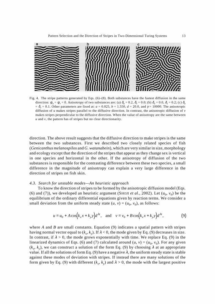
Figure 4 shows stripe patterns generated by Eqs. (6)–(8) when ψu = ψv = 0. Theanisotropic diffusion of u and isotropic diffusion of v produced stripes parallel to thecommon diffusive direction (Fig. 4a). In contrast, the anisotropic diffusion of v andisotropic diffusion of u make stripes perpendicular to the diffusive direction (Fig. 4b).

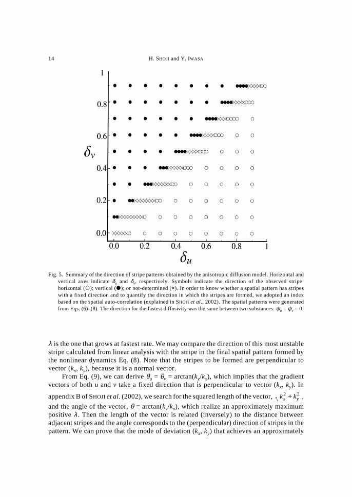
The direction of stripes to be formed depends critically on the relative magnitude ofanisotropy. When anisotropy of u is stronger than that of v (δu ≥ δv), stripes are formedparallel to the diffusive direction, whilst, if anisotropy of v is larger than that of u (δu < δv),the stripes are formed perpendicular to the diffusive direction. Figure 5 shows the summaryof the direction of stripe patterns obtained by the anisotropic diffusion model. Horizontaland vertical axes indicate δu and δv, respectively. Each point indicates the direction of theobserved stripe: horizontal (�); vertical (�); or not-determined (×). This phase plane isseparated into a domain in which stripes were parallel to the diffusive direction (horizontalstripes) and another domain in which stripes were perpendicular to the diffusive direction(vertical stripes). In between these two, there is a narrow band in which the direction ofstripes could not be determined by the algorithm (e.g. in Fig. 4c), indicated by the “×”marks in Fig. 5.

Most of fish species with stripe pattern on their skin have stripes either parallel orperpendicular to their anterior-posterior axis. Very few species has stripes of random


direction. The above result suggests that the diffusive direction to make stripes is the samebetween the two substances. First we described two closely related species of fish(Genicanthus melanospilos and G. watanabein), which are very similar in size, morphologyand ecology except that the direction of the stripes that appear as they change sex is verticalin one species and horizontal in the other. If the anisotropy of diffusion of the twosubstances is responsible for the contrasting difference between these two species, a smalldifference in the magnitude of anisotropy can explain a very large difference in thedirection of stripes on fish skin.

4.3. Search for unstable modes—An heuristic approachTo know the direction of stripes to be formed by the anisotropic diffusion model (Eqs.

(6) and (7)), we developed an heuristic argument (SHOJI et al., 2002). Let (u0, v0) be theequilibrium of the ordinary differential equations given by reaction terms. We consider asmall deviation from the uniform steady state (u, v) = (u0, v0), as follows:

u u A k x k y d v v B k x k y dx yt

x yt= + +( ) = + +( ) ( )0 0 9cos , cos ,λ λand

where A and B are small constants. Equation (9) indicates a spatial pattern with stripeshaving normal vector equal to (kx, ky). If λ < 0, the mode given by Eq. (9) decreases in size.In contrast, if λ > 0, the mode grows exponentially with time. We replace Eq. (9) in thelinearized dynamics of Eqs. (6) and (7) calculated around (u, v) = (u0, v0). For any given(kx, ky), we can construct a solution of the form Eq. (9) by choosing λ at an appropriatevalue. If all the solutions of form Eq. (9) have a negative λ , the uniform steady state is stableagainst these modes of deviation with stripes. If instead there are many solutions of theform given by Eq. (9) with different (kx, ky) and λ > 0, the mode with the largest positive

Fig. 4. The stripe patterns generated by Eqs. (6)–(8). Both substances have the fastest diffusion in the samedirection: ψu = ψv = 0. Anisotropy of two substances are: (a) δu = 0.2, δv = 0.0; (b) δu = 0.0, δv = 0.2; (c) δu

= δv = 0.1. Other parameters are fixed at: a = 0.025, b = 1.550, d = 20.0, and γ = 10000. The anisotropicdiffusion of u makes stripes parallel to the diffusive direction. In contrast, the anisotropic diffusion of vmakes stripes perpendicular to the diffusive direction. When the value of anisotropy are the same betweenu and v, the pattern has of stripes but no clear directionarity.


λ is the one that grows at fastest rate. We may compare the direction of this most unstablestripe calculated from linear analysis with the stripe in the final spatial pattern formed bythe nonlinear dynamics Eq. (8). Note that the stripes to be formed are perpendicular tovector (kx, ky), because it is a normal vector.

From Eq. (9), we can derive θu = θv = arctan(ky/kx), which implies that the gradientvectors of both u and v take a fixed direction that is perpendicular to vector (kx, ky). In

appendix B of SHOJI et al. (2002), we search for the squared length of the vector, k kx y2 2+ ,

and the angle of the vector, θ = arctan(ky/kx), which realize an approximately maximumpositive λ . Then the length of the vector is related (inversely) to the distance betweenadjacent stripes and the angle corresponds to the (perpendicular) direction of stripes in thepattern. We can prove that the mode of deviation (kx, ky) that achieves an approximately

Fig. 5. Summary of the direction of stripe patterns obtained by the anisotropic diffusion model. Horizontal andvertical axes indicate δu and δv, respectively. Symbols indicate the direction of the observed stripe:horizontal (�); vertical (�); or not-determined (×). In order to know whether a spatial pattern has stripeswith a fixed direction and to quantify the direction in which the stripes are formed, we adopted an indexbased on the spatial auto-correlation (explained in SHOJI et al., 2002). The spatial patterns were generatedfrom Eqs. (6)–(8). The direction for the fastest diffusivity was the same between two substances: ψu = ψv = 0.


maximum λ has angle θ = arctan(ky/kx) that maximizes the following quantity:

η θ θθ

δ θ ψ

δ θ ψ( ) = ( )

( )=

− −( )( )− −( )( ) ( )D

Dv

u

u u

v v

1 2

1 210

cos

cos.

See appendix B of SHOJI et al. (2002) for the argument leading to this result. In thefollowing we examine the angle that maximizes Eq. (10), denoted by θpredicted.

When we consider first the case in which the diffusive direction of two substances isthe same (i.e. ψu = ψv), we should examine the maximum of η2 = (1 – δuw)/(1 – δvw), when–1 ≤ w ≤ 1, by setting w = cos(2(θ – ψ)). By drawing the graph of this function, we canconclude as following:

If δu > δv, stripes are formed parallel to the diffusive direction.If δu < δv, stripes are formed perpendicular to the diffusive direction.If δu = δv, there is no specific direction for stripes.This is consistent with the simulation results (SHOJI et al., 2002).

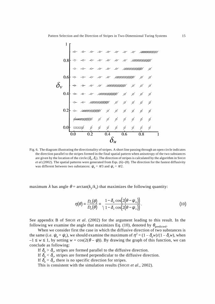
Fig. 6. The diagram illustrating the directionality of stripes. A short line passing through an open circle indicatesthe direction parallel to the stripes formed in the final spatial pattern when anisotropy of the two substancesare given by the location of the circle (δu, δv). The direction of stripes is calculated by the algorithm in SHOJI

et al.(2002). The spatial patterns were generated from Eqs. (6)–(8). The direction for the fastest diffusivitywas different between two substances: ψu = π/3 and ψv = π/2.


4.4. When the diffusive directions differ: ψu ≠ ψvIn the last section, both substances are assumed to have the highest diffusivity in the

same direction. We may also consider the general case in which the direction of maximumdiffusivity can be different between the two substances.

The same method predicts the direction of stripes to form. When anisotropy is smallfor both substances (δu << 1, and δv << 1), by expanding η(θ)2 with eliminating the higherorder terms, SHOJI et al. (2002) predict that the stripe patterns to be formed should have anormal vector with the angle given by

θ δ ψ δ ψδ ψ δ ψ

πpredicted = −

−

+ ( )1

2

2 2

2 2 211arctan

sin sin

cos cos.u u v v

u u v v

When the most diffusive direction is different (not parallel) between the two substances,the direction of stripes changes smoothly from the diffusive direction of u to the directionperpendicular to the diffusive direction of v as the anisotropy of u and v change smoothly.Figure 6 illustrates the direction of the stripes in the final spatial pattern when ψu = π/3 andψv = π/2. The predicted direction is very close to the direction of the stripes observed insimulation results (see figure 5 of SHOJI et al., 2002, in which we compared the predicteddirections with obtained one in case ψu = π/3 and ψv = π/6).

5. Discussion

In this paper, we have reviewed a series of papers on two-dimensional patternformation of Turing systems that are motivated by pattern formation of fish skin (SHOJI etal., 2002, 2003a, 2003b).

First, we discussed the effect of the choice of reaction terms on pattern selection. Weexamined the model with linear reaction terms and additional constraint terms whichconfine the variables within a finite range. We first show that in a one-dimensional model,a periodic stationary pattern can be formed only when activator level is contrained bothfrom below and from above. The constraint of inhibitor is irrelevant. In the two-dimensionalmodel, the relative distance of the equilibrium level of activator between the upper andlower limitations determines the pattern selection. Patterns with stripes are produced whenthe equilibrium is equally distant from the upper and the lower limitations, but patterns withspots are produced when the equilibrium is clearly closer to one than to the other of twolimitations. We then attempt to explain the pattern selection of nonlinear models based onthe result of linear models with constraints. The distribution of activator level is skewedpositively and negatively for spot patterns and reversed spot patterns, respectively. Incontrast, the skewness of the distribution of activator level was small for striped patterns.This gives an intuitive explanation of why the location of the equilibrium betweenconstraints. We then interpreted the pattern selection of nonlinear Turing model, based onthe insights obtained from the result of Turing model with linear reaction and constrants.

Second, we introduced anisotropic diffusion into diffusion term to explain the skinpattern of two closely related species of fish (Genicanthus melanospilos and G. watanabein),which are very similar in size, morphology and ecology except that the direction of the


stripes that appear as they change sex is vertical in one species and horizontal in the other.If the anisotropy of diffusion of the two substances is responsible for the contrastingdifference between these two species, a small difference in the magnitude of anisotropy canexplain a very large difference in the direction of stripes on fish skin. According to thediscussion in this review, such a discontinuous change in the direction of stripes can beobserved only when the direction of anisotropy of the two substances coincides. If thediffusive directions of the two substances are different, we should observe a continuouschange in the directionality of stripes caused by smooth change in parameters. Consideringthe strong similarity of the two species in genus Genicanthus, the theoretical study suggeststhat anisotropy of the two substances expressed in reaction-diffusion model is responsiblefor determining the direction of stripes and that the diffusive direction of the twosubstances must be the same.

Turing models give the basic logic in biological pattern formation. They have beenstudied mathematically over half a century since the seminal paper was proposed (TURING,1952). However in most of these studies, the model stays phenomenological because of ourlack of knowledge on the underlying processes of morphogenesis. However the situationis going to change very soon. Thanks to quick development of molecular biology in the laterhalf of the last century, we are going to get detailed molecular basic of pattern formationand development of organisms. This will give us a great opportunity to develop mathematicaland computational models that consider those newly available information and that arefully based on the knowledge of mechanistic basis. We predict that Turing models wouldstill give the basis of the biological pattern formation, and the importance of the Turing ideawill becomes even more clearer as the result of the progress of mathematical study ofbiological pattern formation.

This work was supported in part by a Grant-in-Aid from the Japan Society for the Promotionof Science to Y.I. We are grateful for Professor Shigeru Kondo, Center for Developmental Biology,RIKEN Kobe and Dr. Atsushi Mochizuki, National Institute for Basic Biology, for their help. Wealso thank the following people for their helpful comments: R. Kobayashi, M. Mimura, T. Ohta, A.Sasaki, and S. Tohya.

REFERENCES

ASAI, R., TAGUCHI, R., KUME, Y., SAITO, M. and KONDO, S. (1999) Zebrafish Leopard gene as a component ofputative reaction-diffusion system, Mech. Dev., 89, 87–92.

DILLON, R., MAINI, P. K. and OTHMER, H. G. (1994) Pattern formation in generalized Turing systems I. Steady-state patterns in systems with mixed boundary conditions, J. Math. Biol., 32, 345–393.

DUFIET, V. and BOISSONADE, J. (1992) Conventional and unconventional Turing pattern, J. Chem Phys., 96,664–673.

ERMENTROUT, B. (1991) Stripes or spots? Nonlinear effects in bifurcation of reaction-diffusion equations on thesquare, Proc. R. Soc. Lond., A434, 413–417.

GIERER, A. and MEINHARDT, H. (1972) A theory of biological pattern formation, Kybernetik, 12, 30–39.KOBAYASHI, R. (1993) Modelling and numerical simulations of dendritic crystal growth, PhysicaD, 63, 410–

423.KONDO, S. and ASAI, R. (1995) A reaction-diffusion wave on the marine angelfish Pomacanthus, Nature, 376,

765–768.KUWAMURA, T. and KARINO, K. (1999) Mimicry of fishes, in Mimicry (ed. K. Ueda), pp. 1–15, Tsukiji shokan,

Tokyo (in Japanese).


LYONS, M. J. and HARRIOSON, L. G. (1992) Stripe selection: An Intrinsic property of some Pattern-Formingmodels with nonlinear dynamics, Devel. Dyn., 195, 201–215.

MEINHARDT, H. (1982) Models of Biological Pattern Formation, Academic Press, London.MURRAY, J. D. (1989) Mathematical Biology, 2nd ed., Springer, New York.SCHNACKENBERG, J. (1979) Simple chemical reaction systems with limit cycle behavior, J. Theor. Biol., 81,

389–400.SEEHAUSEN, O., MAYHEW, P. J. and VAN ALPHEN, J. J. M. (1999) Evolution of color patterns in East African

ciclid fish, J. Evol. Biol., 12, 514–534.SHOJI, H., IWASA, Y., MOCHIZUKI, A. and KONDO, S. (2002) The directionality of stripes formed by anisotropic

reaction-diffusion model, J. Theor. Biol., 214, 549–561.SHOJI, H., MOCHIZUKI, A., IWASA, Y., HIRATA, M., WATANABE, T., HIOKI, S. and KONDO, S. (2003a) Origin

of directionality in fish stripe pattern, Devel. Dyn., 226, 627–633.SHOJI, H., IWASA, Y. and KONDO, S. (2003b) Stripes, spots, or reversed spots in two-dimensional Turing system,

J. Theor. Biol. (in press).TURING, A. M. (1952) The chemical basis of morphogenesis, Phil. Trans. R. Soc. Lond., B237, 37–72.YAMAGUCHI, M. (2002) Aqua Life, Marine Planning International, Tokyo (in Japanese).

Documents

Pattern Selection and the Direction of Stripes in Two ... · Here we assume that d is larger than 1, and hence diffusivity of v is larger than that of u. Now we consider the equilibrium