Patterns of Change and Relationships

UNIT OVERVIEW

GOALS AND STANDARDS

MATHEMATICS BACKGROUND

UNIT INTRODUCTION

Mathematics BackgroundPatterns of Change and Relationships

The introduction to this Unit points out to students that throughout their study of Connected Mathematics they have been asked to look for important relationships between variables, to model those relationships with algebraic expressions, equations, and graphs, and to use those representations to solve problems. In every Unit, real-world contexts have been used to motivate and make sense of new knowledge. This Unit, too, begins with real-world situations, in which students decide which quantities to investigate. They use contextual cues, such as measurement units, to make sense of new ideas, such as domain and range and inverse functions.

Working on the Investigations and Problems of this final CMP Unit will extend students understanding of functions and their representations to include new forms of mathematical notation, new families of functions, and new techniques for transforming expressions to equivalent forms and solving equations. It will also present an extension of the real-number system to the complex numbers.

The Unit objectives address a large range of topics to assure that all first-year algebra topics are covered by the CMP eighth-grade Units. These topics extend and complement coverage in the following Units:

• Thinking With Mathematical Models

• Growing, Growing, Growing

• Frogs, Fleas, and Painted Cubes

• It’s In the System

• Say It With Symbols

Students also make productive connections with these geometry Units:

• Looking for Pythagoras and

• Butterflies, Pinwheels, and Wallpaper

The Unit objectives for Function Junction aim for development of student understanding and skill in work with the following mathematical ideas:

• The domain and range of functions and the f (x) notation for expressing functions

• Numeric and graphic properties of step and piecewise-defined functions

• Properties and uses of inverse functions

• Properties and applications of arithmetic and geometric sequences

• Relationships between functions with graphs connected by transformations such as translations and dilations

continued on next page

13Mathematics Background

CMP14_TG08_U8_UP.indd 13 10/01/14 2:46 PM

Look for these icons that point to enhanced content in Teacher Place

• Expression of quadratic functions in equivalent vertex form and use of that new form to solve equations and sketch graphs

• A formula for solving any quadratic equation

• Meaning of and operations on complex numbers

• Use of polynomial expressions and functions to model and answer questions about complicated data patterns and graphs

Function, Domain, and Range

In the algebra strand of the CMP curriculum, students have studied functions often, beginning with the Variables and Patterns Unit of Grade 6, the Moving Straight Ahead Unit of Grade 7, and the various algebraic Units of Grade 8. Those Units have emphasized the concepts of independent and dependent variables and the use of equations such as y = 3x + 7 and the graphs of (x, y) value pairs to represent functions.

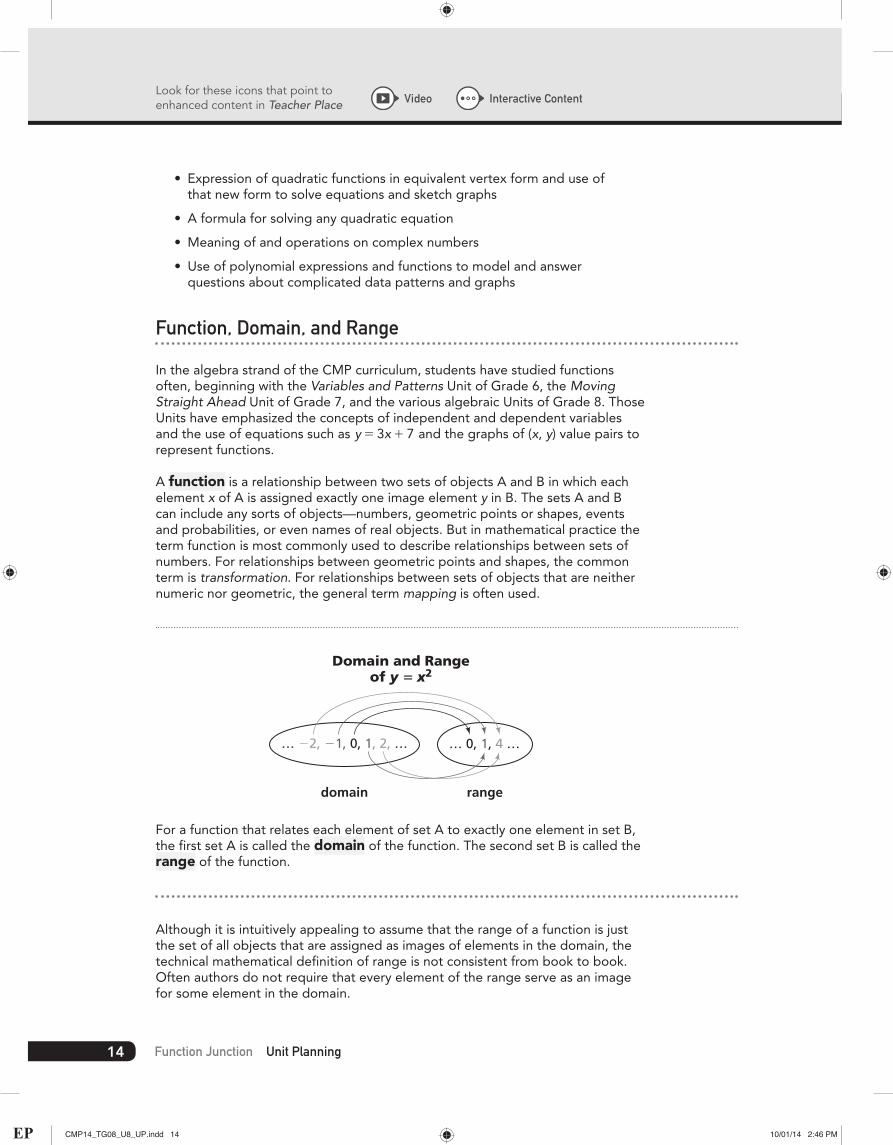
A function is a relationship between two sets of objects A and B in which each element x of A is assigned exactly one image element y in B. The sets A and B can include any sorts of objects—numbers, geometric points or shapes, events and probabilities, or even names of real objects. But in mathematical practice the term function is most commonly used to describe relationships between sets of numbers. For relationships between geometric points and shapes, the common term is transformation. For relationships between sets of objects that are neither numeric nor geometric, the general term mapping is often used.

Domain and Rangeof y = x2

domain range

… −2, −1, 0, 1, 2, … … 0, 1, 4 …

For a function that relates each element of set A to exactly one element in set B, the first set A is called the domain of the function. The second set B is called the range of the function.

Although it is intuitively appealing to assume that the range of a function is just the set of all objects that are assigned as images of elements in the domain, the technical mathematical definition of range is not consistent from book to book. Often authors do not require that every element of the range serve as an image for some element in the domain.

Function Junction Unit Planning14

Interactive ContentVideo

CMP14_TG08_U8_UP.indd 14 10/01/14 2:46 PM

UNIT OVERVIEW

GOALS AND STANDARDS


UNIT INTRODUCTION

On the other hand, some authors call the second set the co-domain of the function and refer to the range as exactly the set of images for elements in the domain— a set that is included in but is sometimes smaller than the co-domain.

For example, the function y = x2 that connects each real number with its square has as its natural domain the set of real numbers. The range or co-domain could also be the set of all real numbers or the set of nonnegative real numbers or a variety of other sets of real numbers (as long as the nonnegative numbers are included). This will be puzzling to many students. Authors who prefer the more inclusive definition of range (making it identical to co-domain) then define another term, image, to indicate the set of all objects that actually serve as images of elements in the domain.

To avoid all of this confusion, CMP uses the more restrictive definition of range as exactly the set of images for domain elements, and nothing extra. If you prefer the other course, you might justify a more inclusive meaning of the term range with this metaphor: If you shoot arrows at a target, every arrow may hit the target, but not all points on the target are hit by arrows!

f (x) Notation

As illustrated in the examples y = 3x + 7 and g(x) = x2 below, it is common to express the rules for function assignments as algebraic equations relating the two variables involved. However, it is also common mathematical practice to use what is known as function notation to record and apply those rules. A statement in the form f (x) = 3x + 7 asserts that for each value of a variable x the associated value of a variable y can be calculated by substituting the value of x in the function rule.

Function Notation

f(x) = 3x + 7

f(5) = 3 ∙ 5 + 7 = 15 + 7 = 22

g(x) = x2

g(5) = 25g(–5) = 25

Meaning

For any valueof x, the functionf(x) gives a singlevalue of y.

For an x-valueof 5, the functionf(x) gives a y-value of 22.

For an x-valueof 5 or –5, g(x)gives a valueof 25.



CMP14_TG08_U8_UP.indd 15 10/01/14 2:46 PM


There may be confusion about the interpretation of the function notation f (x) as “f times x,” since students have been using parentheses as an algebraic representation of multiplication. In the probability Unit What Do You Expect, students use parentheses to indicate probability of an invent occurring. For example, P(getting a head), or P(H), means the probability of getting a head on a toss of a coin. The parentheses do not indicate multiplication. Usually the context will make clear when function notation is intended and when algebraic multiplication is intended.

It should not be surprising if you find many students asking, “Why do we have to use this new notation?” When they are asked a set of questions involving function notation, you may find them replacing each occurrence of f (x) with the single letter y. The clearest early advantage of the new notation is that f (5) or g(-5) is convenient shorthand for the longer sentence “Find the value of y when x = 5,” or “Find the value of y when x = -5.”

Students will encounter some other convenient uses of function notation in Investigation 2 when they are asked to analyze sequences and express relationships between successive terms with equations relating f (n) and f (n + 1). Again, these notations are more succinct expressions of statements about relationships between terms of a sequence. (The subscript notation yn and yn+1 is also commonly used to relate successive terms, as shown in the Example.)

Example

Function Notation Subscript Notation

f(n)f(n + 1)f(n + 2)

ynyn+1yn+2

Similarly, function notation proves convenient in Investigation 3 when questions are asked about horizontal translation and stretching of function graphs. Such questions can be expressed as f (x { k) = ■ and g(kx) = ■.

Function notation is also the standard for expressing ideas in calculus.

Step and Piecewise-Defined Functions

Almost all of the functions that CMP students have encountered in prior algebra Units can be expressed with relatively simple algebraic expressions and smooth continuous graphs. (These are graphs with no sharp corners, which can be traced without lifting one’s pencil from the paper, as in the figure on next page.)



CMP14_TG08_U8_UP.indd 16 10/01/14 2:46 PM

UNIT OVERVIEW

GOALS AND STANDARDS


UNIT INTRODUCTION

Height

Time

There are a number of practical and theoretical situations in which a function of interest has a graph that is neither smooth nor continuous. In fact, many of the situations modeled with functions that have smooth linear or quadratic graphs actually involved changes of variables that occur in jumps. Other functions can be represented not only with familiar algebraic rules, but also with different rules on different parts of their domains, as in the figure below. Problems 1.3 and 1.4 introduce examples of such step and piecewise-defined functions.

Height

Time

Step FunctionsSuppose that the domain of a function f (x) is an interval on the number line that has been partitioned into disjoint subintervals, and that on each subinterval the function takes on a different constant value. Then f (x) is called a step function.

The name step function comes from the fact that graphs of such functions look somewhat like staircases. It is not important that students learn a technical definition of step functions, only that they become aware that some useful functions behave quite differently than the basic families that have been the focus of attention in prior algebra Units. The graph below shows the standard rounding function.

O

y

x

�2 �1 1 2

�2

�1

1

2



CMP14_TG08_U8_UP.indd 17 23/01/14 5:39 PM


The graph above shows values of the function that matches each real number between - 3 and 3 with its nearest integer. How does the function behave at the discontinuity points - 2.5, - 1.5, - 0.5, 0.5, 1.5, and 2.5? The standard rounding rule rounds up. This behavior at the ends of the steps is commonly indicated by drawing an open dot at the right end of each graph segment and a solid dot at the left end of each graph segment.

This convention is similar to that for indicating segments on a number line corresponding to inequalities. The graph below shows the inequality 3 … x 6 5. It has a closed dot at x = 3 and an open dot at x = 5.

0 1 2 3 4 5 6−1

3 ≤ x < 5

In other step function examples, the behavior at discontinuity points might be different. But the technique of indicating what happens at those discontinuity points is the same—solid dots for actual function values and open dots for points not on the graph of the actual function.

Piecewise-Defined FunctionsIn some situations for which algebraic function models would be useful, the behavior of the related variables is such that different rules relate the variables on different parts of the domain.

Suppose a car drives at a speed of 30 miles per hour for five minutes and then at a higher speed of 60 miles per hour for ten minutes more. The graph showing distance as a function of time will have two straight pieces with different slopes—0.5 mile per minute for the first segment and 1.0 mile per minute for the second segment. While a very accurate model would have to account for some period of acceleration from 30 to 60 mph, a line with pieces of different slope would be a reasonably accurate model. The graph below represents distance as a function of time.

50

Time (minutes)

5

0

10

15

Dis

tan

ce (

mile

s)

10

d(t) = t – 2.5

d(t) = 0.5t

15

Speed is 1.0 mile per minute.

Speed is0.5 mileper minute.



CMP14_TG08_U8_UP.indd 18 23/01/14 5:39 PM

UNIT OVERVIEW

GOALS AND STANDARDS


UNIT INTRODUCTION

Because the function has different rules on different parts of its domain, it is said to be a piecewise-defined function, or simply a piecewise function. Once again, it is not critical that students learn a technical definition of such functions, only that they realize such relationships can indeed satisfy the definition of a function and that they can be quite useful models for problem situations.

Inverse Functions

Consider the two linear functions f (x) = 3x + 7 and g(x) = x - 73 and their effects on

some sample pairs of values:

f (0) = 3(0) + 7 and g(7) = 7 - 73

f (0) = 7 and g(7) = 0

f (1) = 10 and g(10) = 1

f (4.5) = 20.5 and g(20.5) = 4.5

f ( - 6) = - 11 and g( - 11) = - 6

In general, if f (a) = b, then g(b) = a.

Because of the special relationship between the two functions, g is called the inverse function of f.

DefinitionIn general, if f is a function with domain A and range B, g is a function with domain B and range A, and g(f (x)) = x for all x in A, then g is the inverse of f.

The function g reverses the assignments of f, and this operation can be very useful in answering questions about the original function. For example, suppose that a school fundraising project sells spirit week T-shirts for +10 apiece. The function f (x) = 10x gives income from the sale of x shirts. The inverse function g(x) = x

10 tells the number of shirts sold if the income is +x.

Terms and NotationThe fundraiser income example illustrates the rationale for using the term inverse to describe the relationship between the two functions. It connects with students’ earlier experience in describing multiplication and division as inverse operations. (Addition and subtraction are also inverses.)

It is quite possible that students will confuse an inverse functions with inverse variation functions (which have rules in the form f (x) = k

x. Make sure that they recognize that the -1 in the inverse function f -1(x) is not an exponent. In other words, it is in general not true that f -1(x) = 1

f (x). You and your students will have to train yourselves to remember that meaning depends on context.



CMP14_TG08_U8_UP.indd 19 10/01/14 2:46 PM


Clarifying NotationOne final issue in notation for inverse functions has to do with letter names of variables. In the T-shirt example described above, it would be natural to use the variables I and n to indicate income and number of sales. It is helpful to use I as the name of the income function as well, so I(n) = 10n. What does one write for the inverse function? The domain of I is the set of whole numbers of T-shirts and the range is the set of multiples of +10. The inverse function I -1 does not operate on the variable n, so I-1(n) does not make sense.

There are at least two ways to avoid this notational confusion. One is to avoid function notation and simply write the relationships between variables in equation form (below left). Another is to use generic function notation and connect to the variables (below right)

Without FunctionNotation

With GenericFunction Notation

I = 10nn = I

10

I = f(x) = 10xn = f –1(x) = x

10

In the second approach, the letter x is simply being used to show how one uses values of the input variable of the function to calculate outputs, not to indicate any particular variable. So the x in f (x) = 10x is referring to a different variable than the x in f -1(x) = x

10.

Restricted Domain and RangeEvery linear function has domain and range that are all real numbers, and every nonconstant linear function has an inverse with the same domain and range. However, finding inverses for many nonlinear functions introduces complications that require care in defining domains and ranges.

For example, the basic quadratic function q(x) = x2 is has all real numbers as its domain. The function, however, takes on only nonnegative real-number values as its range. Furthermore, if one is told that q(x) = 9, the value of x could be either 3 or -3. The inverse relation q-1(x) is not well defined, as shown below.

O 1 2 3 4

−2

−1

1

2y

x



CMP14_TG08_U8_UP.indd 20 10/01/14 2:46 PM

UNIT OVERVIEW

GOALS AND STANDARDS


UNIT INTRODUCTION

If one restricts the domain of q(x) = x2 to the nonnegative real numbers, then q-1(x) = 2x is unambiguous and the inverse function is well defined.

Domain restrictions are needed to assure well-defined inverses for some other familiar functions.

ExampleThe function v(x) = ƒx ƒ , below, has as its natural domain all real numbers, but an inverse can only be well defined if the domain is restricted to either the nonnegative or the nonpositive numbers.

O–1–2 21

1

2

v(x)

x

Finding Rules for Inverse FunctionsAs a practical matter, in finding inverse function rules, the equation format for function representation is generally most helpful. For example, if y = 3x + 7, then finding the inverse means finding a way to calculate x when given y. Solving

the given equation for x in terms of y yields x = y - 73 . So if y = 3x + 7, then

f -1(x) = x - 73 . Once again, the generic use of the letter x to indicate the

input variable for any function might be puzzling to students who have grown accustomed to thinking about variables as numbers with context.

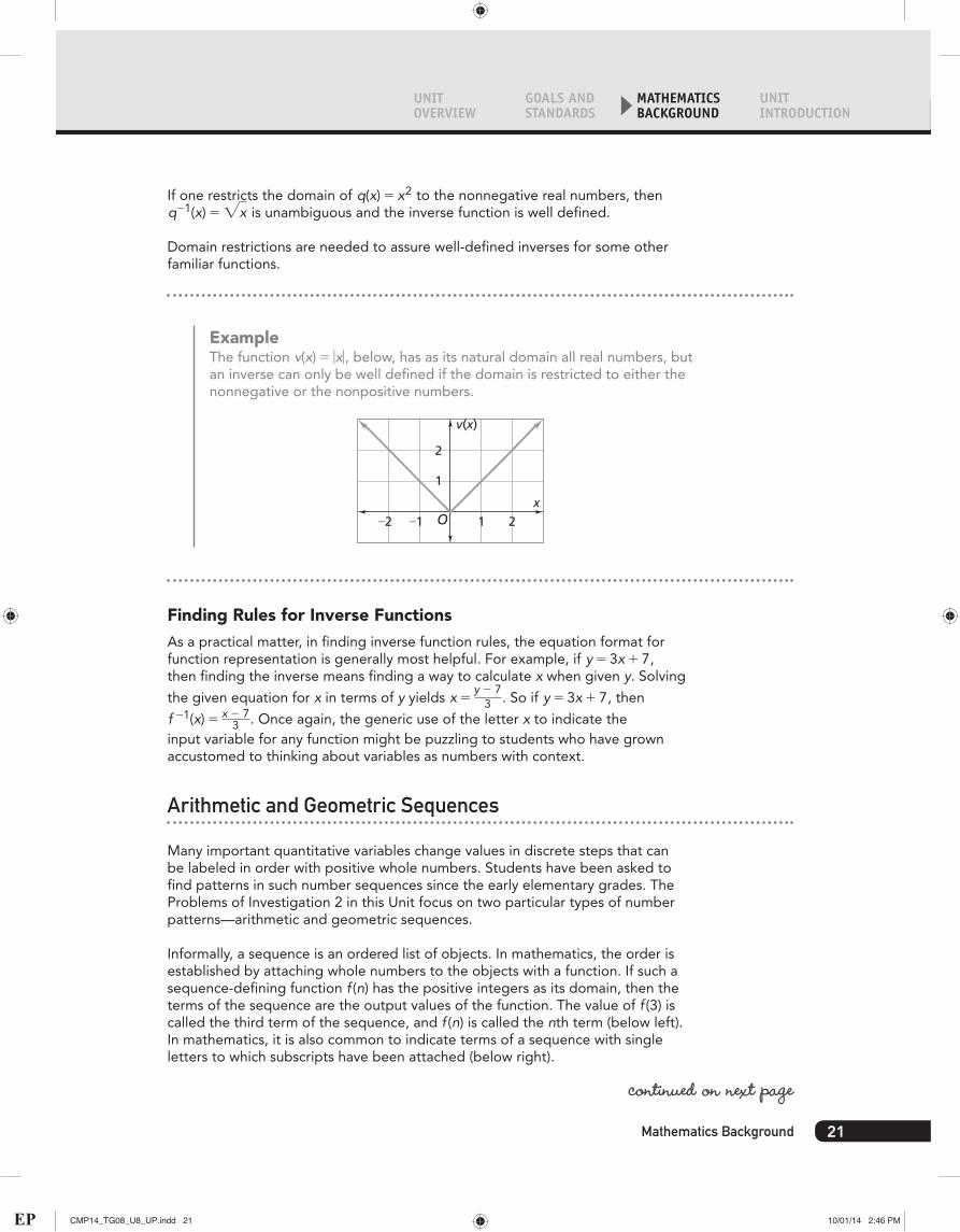
Arithmetic and Geometric Sequences

Many important quantitative variables change values in discrete steps that can be labeled in order with positive whole numbers. Students have been asked to find patterns in such number sequences since the early elementary grades. The Problems of Investigation 2 in this Unit focus on two particular types of number patterns—arithmetic and geometric sequences.

Informally, a sequence is an ordered list of objects. In mathematics, the order is established by attaching whole numbers to the objects with a function. If such a sequence-defining function f (n) has the positive integers as its domain, then the terms of the sequence are the output values of the function. The value of f (3) is called the third term of the sequence, and f (n) is called the nth term (below left). In mathematics, it is also common to indicate terms of a sequence with single letters to which subscripts have been attached (below right).



CMP14_TG08_U8_UP.indd 21 10/01/14 2:46 PM


Function Notation Subscript Notation

f(1), f(2), f(3),… f(n) y1, y2, y3,… y(n)

Third term

nth term

In much of mathematics, the word sequence means a list with an infinite number of terms. A list with a finite number of terms is generally called a finite sequence. However, there is no reason here to make this distinction with students. You may use the term sequence to mean either an “infinite” or a “finite” list, for which the term finite sequence can be used for emphasis in cases in which the list is obviously intended to be finite.

An arithmetic sequence is a sequence of numbers with the property that the difference between successive terms is constant. This relation can be written as f (n + 1) - f(n) = k for all n and some constant number k (below left).

A geometric sequence is a sequence of numbers with the property that the ratio of successive terms is constant or that g(n + 1) , g(n) = k for all n and some constant number k (below right). Students will probably quickly notice the patterns in examples of the two types of sequences. These rules, which define each term of a sequence as a function of the previous term, are called recursive rules.

Arithmetic Sequence Geometric Sequence

f(n + 1) = f(n) + k g(n + 1) = g(n) ∙ k

The number pattern that begins 0, 10, 20, 30, 40, 50, . . . has a fourth term f (4) = 30, and this list appears to be the start of an arithmetic sequence with constant difference 10 between successive terms. In elementary mathematics courses, the expected answer is that the sequence will continue as 60, 70, 80, and so on. However, students might see different continuation patterns depending on prior experience. In fact, if one thinks of the pattern as yard markers on a football field, the next terms would be 40, 30, 20, 10, and 0.

For any arithmetic sequence, there is a closed-form rule for finding the value of the nth term (below left). For any geometric sequence, there is a closed-form rule for finding the nth term (below right).

Closed-Form Rule forArithmetic Sequence

Closed-Form Rule forGeometric Sequence

f(n) = f(1) + (n – 1)b f(n) = f(1)bn–1



CMP14_TG08_U8_UP.indd 22 10/01/14 2:46 PM

UNIT OVERVIEW

GOALS AND STANDARDS


UNIT INTRODUCTION

These two sequence formulas are, of course, special cases of linear and exponential functions, with the domain restricted to positive whole numbers.

In many applications of arithmetic or geometric sequences, it is natural to be interested not only in the individual terms, but in the sums of terms. For any sequence with terms a(1), a(2), a(3), . . . there is a related sequence of partial sums S1, S2, S3, . . . The terms in that associated sequence are defined as follows:

S1 = a(1)

S2 = a(1) + a(2)

S3 = a(1) + a(2) + a(3)

and so on.

We address the concept of arithmetic and geometric series only in Extension Exercises 29 and 30 of Investigation 2. Not surprisingly, there are formulas for calculating the terms of both kinds of sequences.

FormulasFor an arithmetic sequence with terms a(1), a(2), a(3), . . . the nth term of the related sequence of partial sums is as below.

Sn = n2 [2a(1) + (n - 1)d] = n(a(1) + a(n)

2 )The sum of the first n terms of any geometric sequence with first term a(1) and common ratio r relating successive terms is given by the formula Sn = a(1)(1 - r n

1 - r ) . The derivation of these formulas is an appropriate topic for an advanced algebra course.

Transforming Graphs, Expressions, and Functions

The overarching goal of Problems in Investigation 3 of this Unit is to show how many families of functions can be derived from and related to a small number of simple examples.

ExampleIn nearly every branch of mathematics there are some basic elements from which the richness of other examples can be derived. The whole numbers can be generated from 1 by successive addition of 1 or from the prime numbers by multiplication. All convex polygons can be partitioned into triangles. Probabilities of compound events can be calculated by arithmetic operations on simple events in a sample space.



CMP14_TG08_U8_UP.indd 23 10/01/14 2:46 PM


The graph and expression of any linear function represent the effects of transforming y = x. The graph and expression of any quadratic function represent the effects of transforming y = x2, and so on.

With an eye on future developments, the examples in Investigation 3 emphasize transformative effects on quadratic functions and their graphs. These ideas were explored in Butterflies, Pinwheels, and Wallpaper, Moving Straight Ahead, and Stretching and Shrinking. But the principles involved are quite general, as is shown below. Visit Teacher Place at mathdashboard.com/cmp3 to see the image gallery.

If the graph of a function g(x) can be obtained from that of a function f(x) by a verticaltranslation with the rule (x, y) (x, y + k), then the rules for the two functions are relatedby the equation g(x) = f(x) + k.

In this example, the graph of g(x)can be obtained from that of f(x) bytranslating the graph of f(x) down 5units. So, f(x) = x2, k = –5, andg(x) = x2 + (–5), or g(x) = x2 – 5.

O

y

O–4 –2

4

2

–4

–2

2 4

xf(x) = x2

g(x) = x2 – 5

1. Vertical Translation: g(x) = f(x) + k

O

y

O–4 –2

4

2

–4

–2

2 4

x

f(x) = x2

g(x) = – 2x2

If the graph of a function g(x) can be obtained from that of a function f(x) by a vertical stretchor shrink with the rule (x, y) (x, ky), then the rules for the two functions are related by theequation g(x) = kf(x). In the case that k is negative, the transformation also involves reflectionacross the x-axis, but the relationship of function expressions is the same.

In this example, the graph of g(x) can beobtained from that of f(x) by verticallystretching the graph of f(x) by a factorof –2. So, f(x) = x2, k = –2, and g(x) = –2x2.

Note: If �k� > 1, multiplying the y-value of each point by k causes the points on the transformedgraph to be farther from the x-axis than those on the original graph are. This results in a graphthat is stretched vertically. Students may struggle to see this as a stretch because the resultinggraph appears narrower than the original.Conversely, if �k� < 1, the points on the transformed graph are closer to the x-axis than those onthe original graph, resulting in a vertical shrink.

2. Vertical Stretch or Shrink: g(x) = kf(x)



CMP14_TG08_U8_UP.indd 24 10/01/14 2:46 PM

UNIT OVERVIEW

GOALS AND STANDARDS


UNIT INTRODUCTION

If the graph of a function g(x) can be obtained from that of a function f(x) by a horizontaltranslation with the rule (x, y) (x + k, y), then the rules for the two functions are relatedby the equation g(x) = f(x – k).

In this example, the graph of g(x)can be obtained from that of f(x) bytranslating the graph of f(x) 3 unitsto the right. So, f(x) = x2, k = 3, andg(x) = (x – 3)2.

O

y

O–4 –2

4

2

–4

–2

2 4

x

f(x) = x2

g(x) = (x – 3)2

3. Horizontal Translation: g(x) = f(x – k)

If the graph of a function g(x) can be obtained from that of a function f(x) by a horizontal stretchor shrink with the rule (x, y) (kx, y), then the rules for the two functions are related by the

equation g(x) = f . In the case that k is negative, the transformation also involves reflection

across the y-axis, but the relationship of function expressions is the same.

In this example, the graph of g(x) can beobtained from that of f(x) by horizontallyshrinking the graph of f(x) by a factor of

–2. So, f(x) = x2, k = –2, and g(x) = .

The original parabola has y-axis symmetry,so its location is the same before andafter the reflection across the y-axis.

Note: If �k� > 1, the points on the transformed graph are farther to the left or right of the axis ofsymmetry than those on the original graph are. This results in a graph that is stretched horizontally.Conversely, If �k� < 1, the graph shrinks horizontally.

xk( )

x–2( )

2

O

y

O–4–6 –2

4

2

–4

–2

2 4 6

xf(x) = x2

6

g(x) = x–2( )

2

4. Horizontal Stretch or Shrink: g(x) = f xk( )



CMP14_TG08_U8_UP.indd 25 10/01/14 2:46 PM


The graph of g(x) can be obtained from the graph of f(x) = x2 through a horizontal translation, avertical stretch and reflection over the x-axis, and a vertical translation.

In this example, the graph of g(x) can beobtained from that of f(x) by translatingthe graph of f(x) 3 units to the left,vertically stretching it by a factor of –2,and then translating it up 1 unit. So, theequation of the resulting graph isg(x) = –2(x + 3)2 + 1.

O

y

O–4–6 –2

4

2

–4

–2

2 4 6

x

f(x) = x2

g(x) = –2(x + 3)2 + 1

6

5. Combination

When writing the equation for a transformed graph, students need to consider the order in whichthe transformations take place. The order of the transformations can affect the resulting graph.

In this example, vertically stretching thegraph of f(x) by a factor of 4, thentranslating it 3 units to the right, andthen translating it 1 unit down results inthe graph of g(x).

However, translating the graph of f(x)3 units to the right, then translating it1 unit down, and then verticallystretching it by a factor of 4 results in thegraph of h(x).

Note: In Function Junction, when writing an equation for a transformed graph, students shouldfirst address any stretching or shrinking and then consider translations.

O

y

O–4–6 –2

4

2

–4

–2

2 4 6

x

f(x) g(x)

h(x)

6

6. Common Student Errors

In the case of the basic linear and quadratic functions y = x and y = x2, the effects of horizontal stretching and shrinking transformations of graphs and expressions can be accomplished as well with vertical stretching and shrinking transformations.

ExampleWhen the graph of f (x) = x2 is stretched horizontally by a factor of 2, the new graph has rule g(x) = (x

2) = 0.25x2. The same result could be obtained with a vertical shrink by a factor of 0.25. When the graph of h(x) = x is shrunk horizontally by a factor of 0.5, the new graph has rule j(x) = ( x

0.5) = 2x. The same result could be obtained with a vertical stretch by a factor of 2.

For these reasons, and because the most powerful use of horizontal stretching or shrinking of graphs and expressions occurs in dealing with changes of period for trigonometric functions, we have addressed the horizontal stretch or shrink case only in Extension exercises of this Unit.



CMP14_TG08_U8_UP.indd 26 10/01/14 2:46 PM

UNIT OVERVIEW

GOALS AND STANDARDS


UNIT INTRODUCTION

Vertex Form of Quadratics

So far in their study of quadratic expressions and functions, students have learned how both standard trinomial forms (for example, x2 + 5x + 6) and factored forms (for example, (x + 2)(x + 3)) reveal important information about the related functions and their graphs. The equation x2 + 5x + 6 and its graph are shown below.

Standard Form and Graphof Quadratic Function

0

1

−1−2−3−4−5 0

2

3

4

5

y = x2 + 5x + 6

y-intercept

x-intercepts

constantterm = 6

leadingcoefficient = 1

linearcoefficient = 5

The leading coefficient in the standard trinomial form determines whether the graph will have a maximum or minimum point. (A positive leading coefficient indicates a minimum, and a negative leading coefficient indicates a maximum.) The coordinates of the y-intercept will be determined by the constant term ((0,6) in the example above). In factored form, the linear factors can be used to quickly find the x-intercepts of the graph or zeros of the function (x = -2 and x = -3 in the example above).

By focusing attention on how transformations of the basic quadratic y = x2 lead to transformed graphs, the first three Problems of Investigation 3 give clues to the form and location of the graph for quadratic functions expressed in what is called vertex form: y = a(x - h)2 + k



CMP14_TG08_U8_UP.indd 27 10/01/14 2:46 PM


Completing the Square and the Quadratic Formula

While the vertex form of a quadratic expression is very useful, once obtained, it is not a trivial task to take any standard trinomial form and transform it to equivalent vertex form. The process is called completing the square, because the tricky part is generating the (x - h)2 perfect square term.

When you try to express a quadratic trinomial in equivalent form as a product of linear factors, there are several possible outcomes. In some cases the result is two different factors, as in this case.

x2 + 6x + 5 = (x + 5)(x + 1)

In a very few instances, the result will be two identical linear factors, as here.

x2 + 6x + 9 = (x + 3)(x + 3)

= (x + 3)2



CMP14_TG08_U8_UP.indd 28 23/01/14 3:26 PM

UNIT OVERVIEW

GOALS AND STANDARDS


UNIT INTRODUCTION

The video below gives a geometrical interpretation of a perfect square trinomial. Visit Teacher Place at mathdashboard.com/cmp3 to see the complete video.

In most instances, however, it is not possible to write a quadratic expression as the product of two identical linear factors. Visit Teacher Place at mathdashboard.com/cmp3 to see the complete video.



CMP14_TG08_U8_UP.indd 29 10/01/14 2:46 PM


For the cases that lead to two different linear factors, it is still possible to write the given quadratic in equivalent vertex form and reap the benefits of that expressive form. The result is the Quadratic Formula, which gives a solution to any quadratic equation.

x = -b2a { 2b2 - 4ac

2a

In this formula, a is the coefficient of the x2 term, b is the coefficient of the x term, and c is the constant term.

Deriving this equation involves some maneuvering that is far from obvious, as is shown below.

Add the term to both

sides of the equation and

rewrite it in equivalent form

to get a common denominator.

( )2b

2a

Taking the square root gives

two values of x + , one

positive and one negative.

Subtracting from both sides

of the equation leaves x by itself.

1. ax2 + bx + c = 0

Combining terms gives the usual

form of the quadratic formula.

8. x = –b ±√ b2 – 4ac

2a

Solving a quadratic equation takes more steps when the leading

coefficient is not 1. By completing the square, it is possible to find a

general formula for solving any quadratic equation of the form

ax2 + bx + c = 0.

ba2. x2 + x + = 0c

a Divide by a.

( )2b

a3. x2 + x + –b2a + = 0 c

a( )2b

2a ( )2

–b2a ( )

2b2aAdd ,

which is zero.

( )2b

a4. x2 + x + = –b2a

4ac4a2

b2

4a2

( )2

5. =x + –b2a

4ac4a2

b2

4a2 The left side is now

a perfect square.

b2a

6. = ±x + –b2a

4ac4a2

b2

4a2√

b2a7. ±x = – –b

2a4ac4a2

b2

4a2√



CMP14_TG08_U8_UP.indd 30 10/01/14 2:46 PM

UNIT OVERVIEW

GOALS AND STANDARDS


UNIT INTRODUCTION

Thus, to solve any quadratic equation, students need only substitute values from the given quadratic trinomial into the formula. They need to keep in mind that a is the coefficient of the x2 term, b is the coefficient of the x term, and c is the constant term.

Complex Numbers

As the Student Edition says, the quadratic formula gives an algorithm for solving any quadratic equation in the form ax2 + bx + c. However, when you use the formula to solve even fairly simple equations such as x2 + 4x + 5, you get some very strange results. According to the quadratic formula, the solutions to that equation should be these two:

x = -2 + 1-42 x = -2 - 1-4

2

The formula says that to find the solutions for x2 + 4x + 5 we must somehow calculate the square root of a negative number!

The graph of f (x) = x2 + 4x + 5 shows the problem from another view. The parabola does not cross the x-axis, so it seems to have no solutions.

0−1−2−3−4 0

2

1

3

4

f(x) = x2 + 4x + 5

This equation has nox-intercepts, so ithas no real solutions.

The kind of seemingly impossible calculation required to solve x2 + 4x + 5 puzzled mathematicians until they decided that what was needed was an extension of the number system. The process began with defining a solution to the very simple equation x2 + 1 = 0. If x2 + 1 = 0, then x2 = -1. So x = { 1-1.

If even that simple quadratic equation is to have a solution, we need a new number whose square is equal to -1. Because all previous mathematics had suggested the impossibility of such a number, the new number was given the label i and called imaginary. The numbers i, 3i, and -8i are imaginary numbers.

If the number system is to be extended to include a number i with the property that i = -1, then some other numbers must be added as well, numbers such as 3i, 5 + 3i, (3i)2, 2(i + 3i), - i, and many others. They are the complex numbers.



CMP14_TG08_U8_UP.indd 31 10/01/14 2:46 PM


In developing operations on complex numbers mathematicians made some assumptions about how the new numbers ought to behave. For example, assuming that the commutative, associative, and distributive properties carry over, one can reason as follows:

Addition

(a + bi ) + (c + di ) = (a + c) + (b + d )i

Multiplication

(a + bi )(c + di ) = (a + bi )c + (a + bi )(di ) Distributive Property

(a + bi )(c + di ) = (ac + bci) + (adi - bd) Distributive Property

(a + bi )(c + di ) = (ac - bd) + (bc + ad)i Simplify.

The results show algorithms for addition (and subtraction) and multiplication of any two complex numbers. They also indicate why any complex number can be expressed in this basic form.

(real number) + (real number)i

• The real numbers are embedded in the complex number system as numbers in the form a + bi.

• Each complex number a + bi is defined by an ordered pair of real numbers a and b, so it is possible to represent any complex number as a point on a two-dimensional coordinate grid.

• The operations of addition (and subtraction) and multiplication (and division) have geometric interpretations. Addition and subtraction can be conceived as translations, with the second number telling how to slide from the first number. The figure below illustrates adding (4 + 2i) and (-1 + 4i ).

x

y

6

4

2

00 2 4

4 + 2i

3 + 6i = (4 + 2i) + (–1 + 4i)

6

• The geometric interpretation of complex multiplication involves angles and distances from the origin in a way that is beyond the scope of this introduction.



CMP14_TG08_U8_UP.indd 32 10/01/14 2:46 PM

UNIT OVERVIEW

GOALS AND STANDARDS


UNIT INTRODUCTION

Polynomial Expressions and Functions

Linear and quadratic functions, equations, and graphs are very familiar mathematical tools. But there are many problems when those friendly functions are not good models for patterns in data and graphs. For example, no linear, quadratic, exponential, or inverse variation function has a graph like this:

O

y

x

�4 �2 2 4

�20

�10

10

20

localminimum

localmaximum

Functions with more “hills and valleys” than the parabolic graphs of quadratics have terms involving x3, x4, and higher powers. For example, the function with graph shown above is f (x) = x3 + x2 - 6x + 2.

This function is in the class of functions called polynomials. Any algebraic expression in the form anxn + an-1xn-1 + c + a1x + a0, where n is a whole number and the coefficients, an, an-1, and so on, are numbers, is called a polynomial.

Cubic Polynomial (n = 3)

a3 = 1 a1 = –6

a2 = 1 a0 = 2

f(x) = x3 + x2 – 6x + 2

A polynomial function is one with a rule given by a polynomial expression.



CMP14_TG08_U8_UP.indd 33 23/01/14 3:28 PM


One of the most important characteristics of any polynomial expression is its degree. The degree of a polynomial is the greatest exponent of the variable with a nonzero coefficient. Certain polynomials of low degree have special names. For example, a quadratic polynomial has degree 2, a cubic polynomial degree 3, and a quartic polynomial degree 4.

Knowing the degree of a polynomial helps in predicting the shape of its graph and solutions of related equations. But for polynomials of degree greater than 2, the variety of possible graphs and solutions of equations is substantial.

• A polynomial function of degree 3 can have 0 or 2 maximum or minimum points (hills or valleys on its graph) and it can have 1, 2, or 3 zeros (x‑intercepts on its graph), as shown below.

O−4 −2 2 4

−4

−2

2

4

y

x

minimum

x-intercepts

maximum

f(x) = – x3 – x2 + 2x

• A polynomial function of degree 4 can have 1 or 3 maximum and minimum points (hills or valleys on its graph) and it can have 0, 1, 2, 3, or 4 zeros (x‑intercepts on its graph on its graph), as shown below.

O

y

x�4 �2 2 4

�24

�36

�48

�12

12

24

36

48Anita

x-intercepts

maxima or minima

f(x) = x4 – x3 – 13x2 – x + 12

Polynomials of higher degree have comparably more variety in their graphs.



CMP14_TG08_U8_UP.indd 34 23/01/14 5:39 PM

UNIT OVERVIEW

GOALS AND STANDARDS


UNIT INTRODUCTION

Operations With Polynomials

Algorithms for operations with polynomials are structurally almost identical to those foroperations with numbers expressed in decimal form.

Algebra

(3x3 + x2 + 5x + 4) +

(2x3 + 7x2 + 3x + 5)

3x3 + 2x3 + x2 + 7x2 +

5x + 3x + 4 + 5

(3x3 + x2 + 5x + 4) +

(2x3 + 7x2 + 3x + 5)

(3 + 2)x3 + (1 + 7)x2 +

(5 + 3)x + (4 + 5)

5x3 + 8x2 + 8x + 9

Addition

Write each number inexpanded form.

Use the commutative andassociative propertiesto rearrange terms.

Use the Distributive Property.

Simplify.

Convert back to standard form.

Arithmetic

(3 × 103) + (1 × 102) + (5 × 101) + 4 +

(2 × 103) + (7 × 102) + (3 × 101) + 5

(3 × 103) + (2 × 103) + (1 × 102) +

(7 × 102) + (5 × 101) + (3 × 101) + 4 + 5

3,154 + 2,735

(3 + 2) × 103 + (1 + 7) × 102 +

(5 + 3) × 101 + (4 + 5)

5 × 103 + 8 × 102 + 8 × 101 + 9

5,889

Subtraction follows a parallel algorithm.

If anything, addition and subtraction of polynomials is simpler than the comparable operations

with numbers. There is no need to worry about algebraic regrouping, similar to what is required

in numerical calculations such as 753 + 354 or 753 – 354.

Arithmetic Algebra

3,154 – 2,735(3x3 + x2 + 5x + 4) –

(2x3 + 7x2 + 3x + 5)

Subtraction

[(3 × 103) + (1 × 102) + (5 × 101) + 4] –

[(2 × 103) + (7 × 102) + (3 × 101) + 5]

(3x3 + x2 + 5x + 4) –

(2x3 + 7x2 + 3x + 5)

Write each number inexpanded form.

(3 × 103) – (2 × 103) + (1 × 102) –

(7 × 102) +(5 × 101) – (3 × 101) + 4 – 5

3x3 – 2x3 + x2 – 7x2 +

5x – 3x + 4 – 5

Use properties of operationsto rearrange terms.

(3 – 2) × 103 + (1 – 7) × 102 +

(5 – 3) × 101 + (4 – 5)

(3 – 2)x3 + (1 – 7)x2 +

(5 – 3)x + (4 – 5)

Use the Distributive Propertyto group like terms.

1 × 103 – 6 × 102 + 2 × 101 – 1 x3 – 6x2 + 2x – 1Simplify.

419Convert back to standard

form.



CMP14_TG08_U8_UP.indd 35 10/01/14 2:46 PM


The required algorithm for multiplication of polynomials is also parallel to standard proceduresfor multiplying numbers expressed in decimal numeration.

Arithmetic Algebra

(324)(21) (3x2 + 2x + 4)(2x +1)

6(103) + 8(102) + 4

6,804

(3(102) + 2(101) + 4)(2(101) + 1)

(3(102) + 2(101) + 4) • 2(101) +

(3(102) + 2(101) + 4) • 1

(3x2 + 2x + 4)2x +

(3x2 + 2x + 4)1

3(102)2(101) + 2(101)2(101) +

4 • 2(101) + 3(102) + 2(101) + 4

3x2 • 2x + 2x • 2x + 4 • 2x +

3x2 • 1 + 2x • 1 + 4 • 1

6(103) + 4(102) + 8(101) + 3(102)

+ 2(101) + 46x3 + 4x2 + 8x + 3x2 + 2x + 4

6x3 + 7x2 + 10x + 46(103) + 7(102) + 10(101) + 4

Regroup 7(102) and10(101) as 8(102).

Multiplication

Convert back tostandard form.

Write each numberin expanded form.

Use the DistributiveProperty.

Multiply the firstfactor by each termof the second factor.

Simply usingexponent rules.

Combine like terms.

Division of polynomials is also parallel to division of numbers expressed in decimal numeration. It is typically part of second-year algebra, so it is not included here.



CMP14_TG08_U8_UP.indd 36 10/01/14 2:46 PM

Documents

Patterns of Change and Relationships