Embed Size (px)
Citation preview

Patterns of Crime and Universities: A Spatial Analysis of
Burglary, Robbery and Motor Vehicle Theft Patterns
Surrounding Universities in Ottawa
by
Elise LaRue B.A., Simon Fraser University, 2005
Thesis Submitted in Partial Fulfillment of the Requirements for the Degree of
Master of Arts
in the School of Criminology
Faculty of Arts and Social Sciences
© Elise LaRue 2013
SIMON FRASER UNIVERSITY
Spring 2013
All rights reserved. However, in accordance with the Copyright Act of Canada, this work may be reproduced, without authorization, under the conditions for “Fair Dealing.” Therefore, limited reproduction of this work for the purposes of private
study, research, criticism, review and news reporting is likely to be in accordance with the law, particularly if cited appropriately.

ii
Approval
Name: Elise LaRue
Degree: Master of Arts (Criminology)
Title of Thesis: Patterns of crime and universities: A spatial analysis of burglary, robbery, and motor vehicle theft patterns surrounding universities in Ottawa
Examining Committee:
Chair: William Glackman, Ph.D. Associate Professor and Graduate Program Director
Martin A. Andresen, Ph.D. Senior Supervisor Associate Professor
J. Bryan Kinney, Ph.D. Supervisor Associate Professor
Nahanni R. Pollard, Ph.D. External Examiner Faculty and Program Coordinator Department of Criminology Douglas College
Date Defended: April 12, 2013 _________________________________ ____

iii
Partial Copyright Licence

iv
Abstract
This thesis explores the spatial distribution of crime in Ottawa, Canada in 2006.
Crime pattern theory provides the theoretical framework for examining the relationship
between the rates of burglary, robbery, and motor vehicle theft and the two universities,
University of Ottawa and Carleton University. This thesis uses ArcView 3.3 software to
geocode and spatially join the crime and census data, and uses GeoDa 0.9.5-i software
to conduct a spatial regression procedure that accounts for spatial autocorrelation
between the crime rates and socio-demographic characteristics at the dissemination
area level. This thesis finds support for crime pattern theory and the geometric theory of
crime, as universities are the strongest predictors of the rates of burglary and motor
vehicle theft. This thesis also finds some support for both social disorganization theory
and routine activity theory as a number of the expected relationships between the socio-
demographic and socio-economic variables and crime are observed.
Keywords: Ottawa; university; crime pattern theory; geometric theory of crime; spatial
regression; spatial autocorrelation

v
Dedication
I dedicate this thesis to my husband Daryl, who has patiently waited for me to
finish my degree for almost as long as I have known him.
Thank you for making me dinners while I worked and for giving up our weekends
and evenings together. Most of all, thank you for supporting me and believing in me
even though many times I wanted to give up.
I love you and I am looking forward to moving on to the next part of our lives
together.

vi
Acknowledgements
I want to thank my senior supervisor Martin Andresen, from whom I have learnt
so much and am very grateful. Thank you for helping me find a topic and data for my
thesis and teaching me how to do spatial analysis. I appreciate you being available to
answer all of my questions, even on weekends.
Thank you to my supervisor Bryan Kinney, who inspired me to study
environmental criminology ever since the first course I took in my undergraduate degree.
Thank you for all of your guidance and support along the way.
Thank you to my external examiner Nahanni Pollard. Your insight and
suggestions were very helpful, and it was a pleasure having you on my committee.
Thank you to Pat and Paul Brantingham, whose theories provided the theoretical
framework for my thesis. You are the reason I chose to attend Simon Fraser University
for graduate school. It was a pleasure to learn from and work with both of you and a
valuable experience.
I want to thank my friends from my graduate class, Lauren, Lorinda, and
Adrienne. I am lucky to have made such good friends who encouraged me throughout
my degree.
Finally, I want to thank my parents, Bob and Janet, and my husband Daryl for
their support over the years that enabled me to complete my thesis.

vii
Table of Contents
Approval .......................................................................................................................... ii Partial Copyright Licence ............................................................................................... iii Abstract .......................................................................................................................... iv Dedication ....................................................................................................................... v Acknowledgements ........................................................................................................ vi Table of Contents .......................................................................................................... vii List of Tables .................................................................................................................. ix List of Figures.................................................................................................................. x
1. Introduction ........................................................................................................... 1
2. Theoretical Framework ......................................................................................... 4 2.1. The Development of Environmental Criminology and the Spatial Analysis of
Crime ...................................................................................................................... 4 2.1.1 The Early Theories ...................................................................................... 4 2.1.2 Social Disorganization Theory ..................................................................... 6 2.1.3 Routine Activity Theory ................................................................................ 9 2.1.4 Geometric Theory of Crime ........................................................................ 11 2.1.5 Crime Pattern Theory ................................................................................ 15 2.1.6 GIS and Crime Mapping ............................................................................ 19
3. Literature Review ................................................................................................ 21 3.1. The City of Ottawa ................................................................................................ 21 3.2. Universities and Crime .......................................................................................... 26
4. Methodology ........................................................................................................ 34 4.1. Research Questions and Hypotheses ................................................................... 34 4.2. Data ...................................................................................................................... 35
4.2.1 Unit of Analysis .......................................................................................... 35 4.2.2 Independent Variables: Universities ........................................................... 41 4.2.3 Independent Variables: Socio-Demographic and Socio-Economic
Variables ................................................................................................... 42 4.2.4 Dependent Variables: Burglary, Robbery, and Motor Vehicle Theft ........... 55 4.2.5 Spatial Joining of the Variables .................................................................. 68 4.2.6 Calculating Crime Rates ............................................................................ 69
4.3. Data Analysis ........................................................................................................ 71 4.3.1 Testing for Spatial Autocorrelation ............................................................. 76 4.3.2 Spatial Regression .................................................................................... 80 4.3.3 Crime Maps ............................................................................................... 81
viii
5. Results ................................................................................................................. 82 5.1. Descriptive Statistics ............................................................................................. 82 5.2. Bivariate Correlations ............................................................................................ 83 5.3. Spatial Autocorrelation and Regression ................................................................ 85
5.3.1 OLS Regression of Full Models ................................................................. 85 5.3.2 Spatial Error Regression of Full Models ..................................................... 88 5.3.3 Spatial Error Regression of Final Reduced Models .................................... 91 5.3.4 Crime Maps ............................................................................................... 94
6. Discussion ........................................................................................................... 98 6.1. Findings ................................................................................................................ 98 6.2. Limitations ........................................................................................................... 104 6.3. Implications ......................................................................................................... 109 6.4. Conclusion .......................................................................................................... 111
Reference List ........................................................................................................... 113

ix
List of Tables
Table 1. Research questions ...................................................................................... 34
Table 2. Hypotheses ................................................................................................... 35
Table 3. Comparison between estimated values and the actual values of the census data for dissemination area containing Carleton University ............... 55
Table 4. Ottawa Police Service weekly crime report data ............................................ 63
Table 5. Geocoded dependent variables..................................................................... 67
Table 6. Descriptive statistics for dependent variables at the dissemination area level .............................................................................................................. 82
Table 7. Descriptive statistics for independent variables at the dissemination area level ...................................................................................................... 83
Table 8. Correlations for independent variables .......................................................... 85
Table 9. OLS Spatial regression results (OLS classic full models without spatial error) ............................................................................................................. 86
Table 10. Spatial regression results (full models controlling for spatial error) ................ 89
Table 11. Spatial regression results (final models controlling for spatial error) .............. 91
x
List of Figures
Figure 1. Brantingham’s diagram of nodes, paths, activity space, and awareness space ............................................................................................................ 14
Figure 2. Map of downtown Ottawa and the universities .............................................. 22
Figure 3. Map of dissemination areas in Ottawa included in the analysis ..................... 54
Figure 4. Residual plots for OLS spatial regression (full models) ................................. 87
Figure 5. Residual plots for spatial regression (full models controlling for spatial error) ............................................................................................................. 90
Figure 6. Residual plots for spatial regression (final models controlling for spatial error) ............................................................................................................. 93
Figure 7. Ottawa burglary rate per 1,000 population by dissemination area (2006) ........................................................................................................... 94
Figure 8. Ottawa robbery rate per 1,000 population by dissemination area (2006) ....... 95
Figure 9. Ottawa motor vehicle theft rate per 1,000 population by dissemination area (2006) ................................................................................................... 96
Figure 10. Ottawa all crimes rate per 1,000 population by dissemination area (2006) ........................................................................................................... 97

1
1. Introduction
“Crimes do not occur randomly or uniformly in time or space or society”
(Brantingham & Brantingham, 2008, 79). Research has shown there are geographical
differences in the patterning of crime locations and these patterns vary by the type of
crime (Bottoms, 2007, 537). The spatial analysis of crime uses spatial data to explore
theories of crime and explain these spatial patterns (Brantingham & Brantingham, 1984,
211). “Understanding crime requires concepts and models that can be used to account
for the patterned non-uniformity and non-randomness that characterises real criminal
events” (Brantingham & Brantingham, 2008, 79).
This thesis is an examination of the spatial patterns of crime in the city of Ottawa,
Ontario in relation to Ottawa’s two universities, the University of Ottawa and Carleton
University. Crime pattern theory, incorporating aspects of social disorganization theory,
routine activity theory and geometric theory of crime, is the theoretical framework for
developing a model to account for the affects of socio-demographic and socio-economic
characteristics and the presence of the two universities on the patterning of three types
of crime, burglary, robbery, and motor vehicle theft. Social disorganization theory
focuses on the social and economic conditions as the basis of crime in an area (Anselin,
Griffiths & Tita, 2008, 98; Shaw & McKay, 1942). Routine activity theory focuses on the
occurrence of crime as an outcome of a motivated offender, a suitable target and the
absence of a capable guardian coming together in time and space (Cohen & Felson,
1979). The geometric theory of crime examines the how crimes are distributed in urban
space by understanding the physical environment and human behaviour using concepts
of nodes, paths and edges (Brantingham & Brantingham, 1981, 48; Andresen & Kinney,
2012, 153). Crime pattern theory incorporates the spatial aspects of social
disorganization theory, routine activity theory and geometric theory of crime, and
integrates them into empirical analyses of crime (Andresen, 2006b, 490).
Crime pattern theory combines concepts from these theories and focuses on the
surrounding environment, including the environmental backcloth, crime generators and
crime attractor activities, as mechanisms that bring the motivated offenders and suitable

2
targets come together in time and space (Anselin, Griffiths & Tita, 2008, 98;
Brantingham & Brantingham, 1993b). Criminal activity is a product of the routine
activities of potential offenders and victims as they move through their awareness
spaces between work, school, home, and leisure activities. Certain places can become
high crime locations when the physical and social characteristics of the area increase
the intersection of potential victims and offenders at these locations. Crime generators
and attractors, such as institutions and facilities, bring more people to certain areas
creating opportunities for crime (McCord et al., 2007, 299). The environmental
backcloth, including the socio-demographic and socio-economic make-up of the area,
interacts with a person’s activity space, creating variations in the risk of crime (McCord
et al., 2007, 298). Crime pattern theory is used to examine the influence of activity
nodes, in particular the two universities, on the patterns of crime and the possibility of
the universities acting as crime generators or attractors in the City of Ottawa.
This thesis will attempt to answer four research questions. First, are there
observable spatial patterns for burglary, robbery and motor vehicle theft in Ottawa?
Second, if there are spatial relationships for burglary, robbery, and motor vehicle theft,
are there differences in the relationships between crime types? Third, if there are spatial
relationships for burglary, robbery and motor vehicle theft, are these relationships related
to the socio-demographic and socio-economic characteristics of the area? Finally, if
there are spatial relationships for burglary, robbery and motor vehicle theft, are these
relationships related to the universities?
These research questions are examined using models for the rates of burglary,
robbery, motor vehicle theft and all crimes, containing the socio-demographic variables
and the variables indicating the presence of Carleton University and the University of
Ottawa. ArcView 3.3 is used to geocode the address level crime data and join the crime
data with the census data at the dissemination area level. Spatial autocorrelation and
spatial regression analysis is conducted using GeoDa 0.9.5-i. The purpose of this thesis
is to examine influence of universities as crime generators on the spatial patterns of
crime. This thesis hopes to add to the knowledge on this topic area by examining crime
in relation to universities in the City of Ottawa, Ontario.
Universities can be the location of a variety of types of crime. The parking lots at
universities provide a large number of potential targets for motor vehicle theft. University
sporting events can attract large crowds and encourage drinking and rivalry that can

3
lead to assaults. Student drinking and partying is an issue for many campuses and can
result in noise disturbances, vandalism, and violence. University facilities and
dormitories are also the target of theft and burglary, especially the theft of laptops and
other electronic equipment. Finally, sexual assaults and robberies can occur on
campuses and dormitories at night.
The relationship between universities and crime became the focus of
criminological research in the 1990s, when the Unites States Congress approved the
Student Right-to Know and Campus Security Act. This Act required colleges and
universities to publish statistics for on campus crimes and to make their crime prevention
and security policies and procedures available to the public (Fisher, Sloan, Cullen, & Lu,
1998, 672). In 1997, the Accuracy in Campus Crime Reporting Act revised the security-
reporting requirement to achieve timely and accurate disclosure of campus crime
statistics and security provisions (Fisher et al., 1998, 672). These legislative changes
created an opportunity for academics to use this data to study the trends in crimes on
campuses in the United States (Sloan, 1994; Bromley, 1995; Volkwein, Szelest, &
Lizotte, 1995; Fisher et al., 1998; Henson & Stone, 1999). There were studies
examining the factors influencing crime on campuses prior to these studies (Molumby,
1976; McPheters, 1978; Fox & Hellman, 1985) but this readily available data, combined
with reports of violent incidents on campus, renewed interest in this topic area. In recent
years, there have been fewer studies examining the relationship between crime and
universities, and in particular, a lack of Canadian studies on this topic.
This thesis begins with a discussion of the environmental criminology theories
that lead to development of the theoretical framework, crime pattern theory that
incorporates aspects of social disorganization theory, routine activity theory and
geometric theory of crime. A description of the physical and social characteristics of the
City of Ottawa provides context to the geographic features that can influence crime
patterns. The relevant literature on the topic of university crime patterns is discussed.
The data and methods used to conduct the analysis in this thesis are identified and
evaluated. The results of the analysis are presented. Finally, this thesis ends with an
examination of the implications and limitations of the findings.

4
2. Theoretical Framework
2.1. The Development of Environmental Criminology and the Spatial Analysis of Crime
2.1.1 The Early Theories
Environmental criminology is a group of theories, influenced by sociology,
psychology, geography, political science, and economics, that examine criminal events,
places, and the immediate circumstances in which they occur (Wortley & Mazerolle,
2008, 1-3). Environmental criminology examines spatial crime patterns in terms of
environmental influences and the geographical distribution of offences (Wortley &
Mazerolle, 2008, 1; Bottoms & Wiles, 2002, 620). Environmental criminology is based
on the following premises, that: the immediate physical and social environment
influences criminal behaviour; the distribution of crime in time and space is non-random
and criminal behaviour is dependent upon situational factors; and understanding the role
of the environment in the patterning of crime is useful in the prevention of crime (Wortley
& Mazerolle, 2008, 2). The findings can be used help police and city planning officials
deploy resources and implement crime prevention strategies (Wortley & Mazerolle,
2008, 1).
The spatial analysis of crime dates back to the 19th Century. A. M. Guerry in
1833 and Adolphe Quetelet in 1842 were among the first to analyze and cartographically
map the occurrence of crime. They examined the effects of demographics, seasons,
climate, population, and poverty on the geographical distribution of crime in France and
found consistent regional differences (Einstadter & Henry, 2006, 128; Herbert, 1982, 31).
They found spatial distributions of crime across the country, with high crime rates in
some areas and low crime rates in others, differences in violent and property crime
rates, and stability of crime rates over time (Paulsen & Robinson, 2004, 55). In England
in the mid-19th Century, other researchers such as Joseph Fletcher, John Glyde and R.
W. Rawson examined crime rates and population statistics. Rawson, for example, in
1839 examined the relationship between census demographics and crime and found
that crowded urban populations were associated with crime (Decker, Shichor, & O’Brien,

5
1982, 14). In 1856, Glyde found crime rates varied with population density (Einstadter &
Henry, 2006, 128). In 1848, Fletcher found crime occurred in areas containing criminal
populations (Einstadter & Henry, 2006, 128).
At the turn of the 20th Century in Chicago, there was extensive foreign
immigration, high rates of juvenile delinquency, and other social problems. The
breakdown of standards, values and alienation resulted in high levels of mobility of
residents, high population turnover, culture conflict, and social instability (Paulsen &
Robinson, 2004, 54). Sociologists questioned how some neighbourhoods remained high
crime areas despite the turnover of populations, and if there was something criminogenic
within the environment that caused crime (Einstadter & Henry, 2006, 130). In the 1920s
and 1930s, researchers in Chicago focused on ecological conditions and intra-city crime
patterns from a sociological perspective. In 1921 Robert E. Park formed, what was later
described, as the human ecological theory in which the city was seen as a living
organism (Park & Burgess, 1969, 24; Paulsen & Robinson, 2004, 57). Human ecology
was the study of the spatial and temporal relationships between human beings and their
environment (Brantingham & Brantingham, 1984, 305; Decker et al., 1982, 13).
Communities had functionally specialized areas within the industrial economy, they
worked together for common goals and competed for scarce resources (Park & Burgess,
1969, 519-521). The patterning of communities was determined by competition;
changes were due to the invasion of new groups into the area, and social succession
(Park & Burgess, 1969, 544).
In 1925, Earnest W. Burgess used human ecology to develop his concentric
circles theory that divided Chicago into five zones that he hypothesized could be applied
to most other cities. The inner most centre was the non-residential central business
district where the city’s major commercial activity occurred (Brantingham & Brantingham,
1984, 247). The next circle was the zone in transition where there was a mix of
industrial factories and poorer residences (Bottoms, 2007, 531). The zone of working
class homes, the residential zone, and the commuter zone were the next three
residential circles with increasing affluence and social status as you moved out of the
city (Bottoms, 2007, 531). New immigrants would move into the zone in transition as it
contained the cheapest housing, and as they became established and earned money,
they would move outwards (Bottoms, 2007, 531). This process continued with every
new immigrant population. Therefore, the zone in transition had a high residential
6
mobility rate and a heterogeneous population (Bottoms, 2007, 531). Crime was most
likely to occur in zone in transition and decrease with distance from the city centre
(Paulsen & Robinson, 2004, 58; Bottoms & Wiles, 2002, 622). Unfortunately, the
concentric circles model does not fit all cities perfectly.
2.1.2 Social Disorganization Theory
From the 1920s to 1960s, Clifford Shaw and Henry McKay used Park and
Burgess’ theories to examine patterns of juvenile delinquency within cities. They found
that juvenile delinquency rates conformed to regular spatial patterns that decreased with
distance from the city centre (Bottoms, 2007, 531). These patterns were stable over
time, even as the racial composition of the city centre changed over decades (Bottoms,
2007, 531). Transitional areas characterised by economic deprivation and physical
deterioration had population and cultural instability (Bottoms & Wiles, 2002, 622). They
hypothesized that juvenile delinquency resulted from detachment from conventional
groups; weak bonds to society and low social control caused delinquency and crime
(Paulsen & Robinson, 2004, 59). These findings lead to social disorganization theory.
Social disorganization theory is a meso theory as it examines the social
dimension and distribution of crime across neighbourhoods (Wortley & Mazerolle, 2008,
4). Social disorganization theory examines how spatial distributions in poverty,
unemployment, ethic heterogeneity, residential stability, and informal social control can
determine a neighbourhood’s level social organization (Martin, 2002, 132-133). Social
disorganization is caused by a decrease in the influence of existing social rules and
behaviours upon individual members of the group and results in competition, distrust and
a community’s inability to regulate itself with its own values (Shaw & McKay, 1998, 63-
66). Social capital, social cohesion, and collective efficacy are indicators of informal
social control within a neighbourhood. Social capital is community organization and
civic participation in maintaining order in the community (Martin, 2002, 133-134).
Collective efficacy is a mutual trust among neighbours and willingness to intervene to
maintain order (Martin, 2002, 133). Social organization in a neighbourhood decreases
as the original population retreats and the neighbourhood is in transition (Paulsen &
Robinson, 2004, 54). Residents no longer identify with and care for their neighbourhood
(Paulsen & Robinson, 2004, 54). Social disorganization occurs when there are conflicts

7
in values and norms, cultural change, and weakening in primary relationships (Paulsen
& Robinson, 2004, 59).
Social disorganization affects crime rates by decreasing informal social control
networks between neighbours and increasing antisocial behaviour; there is a decrease
in interaction between neighbours and decrease in the ability to maintain effective social
controls (Paulsen & Robinson, 2004, 54). Neighbourhoods, with rapidly changing
compositions, are more likely to experience delinquency and crime than other
neighbourhoods with slower changing compositions (Einstadter & Henry, 2006, 136).
Shaw and McKay (1942) found that physical, economic, and social factors influenced
crime rates (Shaw & McKay, 1998, 63). City centres were characterised by economic
deprivation, cultural heterogeneity, residential instability, and physical deterioration
(Bottoms, 2007, 531). Residential communities characterised by higher socio-economic
status had conventional norms and lower rates of delinquency, whereas urban
communities characterised by lower socio-economic status and larger immigrant and
migrant populations, had greater disparity in values and higher delinquency rates (Shaw
& McKay, 1998, 64-66). Areas with high rates of juvenile delinquency had high industry
and commerce, high levels of foreign-born families, low economic status, and high
welfare levels (Shaw & McKay 1998, 66). Characteristics of communities with social
disorganization include urbanization, mixed land uses, high population density,
residential mobility, high immigrant populations, racial or ethnic heterogeneity, low socio-
economic status, and single parent and female-headed households (Paulsen &
Robinson, 2004, 59).
Some disadvantages of social disorganization theory are that it may only be
relevant to the inner-city environment and urban areas (Paulsen & Robinson, 2004, 72).
It does not explain individual behaviour but variations in crime rates (Paulsen &
Robinson, 2004, 72). Shaw and McKay relied on social, cultural and economic factors to
interpret delinquency, borrowing from the social ecology and concentric circles model;
however, they did not provide evidence of ecological adaptation to different areas
(Herbert, 1982, 36). Another important problem with this theory is it lacks direct
measures for the concepts of social disorganization, social capital, social cohesion, and
collective efficacy, as these concepts are difficult to operationalize (Paulsen & Robinson,
2004, 73). Studies often use socio-economic status, poverty, ethnicity, family and
8
residential stability as indicators of social disorganization (Ceccato & Oberwittler, 2008,
186).
The social ecology approach has been criticised for its reliance on official
definitions and measures of crime and the use of official crime statistics (Einstadter &
Henry, 2006, 130). The use of official crime statistics may reflect policing patterns rather
than actual crime patterns (Einstadter & Henry, 2006, 146). There is an ecological
fallacy of using aggregate level data to draw conclusions for individuals (Einstadter &
Henry, 2006, 145). Finally, social ecology places too much emphasis on simple
demographic, social, and economic indicators which themselves may have complex
relationships to the underlying causes of crime (Einstadter & Henry, 2006, 145).
Social disorganization theory provides the framework for relating most of the
socio-demographic and socio-economic independent variables to crime. Social
disorganization theory hypothesized that low socio-economic status, racial and ethnic
heterogeneity, residential mobility and family disruption, leads to community social
disorganization and increases in crime (Sampson & Groves, 1989, 774). The socio-
demographic and socio-economic characteristics of a population can influence the crime
rate (Andresen, 2006b, 489). As the underlying socio-demographic structure of a
neighbourhood or city changes, the population at risk also changes and influences the
amount of crime in an area (Bruce, Hick, & Cooper, 2004, 263).
Social and economic disadvantage is strongly related to crime, especially
assault, robbery, and homicide (Kitchen, 2006, 8). Studies have found relationships
between crime and low socio-economic status, minority population, proportion of young
males, crowded housing, and proximity to offender residence (Harries, 1980, 90). The
risk of personal victimization is highest in urban areas characterised by single
populations living in low income households, whereas the risk of property victimization is
highest for higher income households (Kitchen, 2006, 8). Ethnic heterogeneity, recent
immigration, unemployment, single parent families, population change and rental
housing are known to have a positive relationship to crime, while education, income and
average value of dwelling are known to have a negative relationship with crime
(Andresen, 2006c, 260; Andresen, 2011a, 397).
Drawing from social disorganization theory, that analyzes groups of people in a
fixed objective space, environmental criminology moves to the analysis of subjective
space (Brantingham & Brantingham, 1984, 332). Subjective space takes into

9
consideration the space as perceived by an individual; spatial behaviour and movement
patterns are complex and depend on underlying spatial mobility knowledge, experience
and biases (Brantingham & Brantingham, 1984, 332). Behaviour is influenced by the
environment; physical, social, psychological, legal and cultural settings all influence
behaviour (Brantingham & Brantingham, 1984, 335-336). This move towards subjective
space leads to the development of routine activity theory and crime pattern theory.
2.1.3 Routine Activity Theory
Cohen and Felson (1979) developed routine activity theory to explain the
increase in property crime that occurred alongside the economic prosperity after the
Second World War. Their work titled “Social change and crime rate trends: A routines
activity approach” described how the dispersion of activities away from the home and
family caused an increase in opportunities for crime (Cohen & Felson, 1979, 588). After
World War II, there was a shift in women working outside of the home and families
travelling out of town, leaving houses and their goods unguarded (Cohen & Felson,
1979, 593). There was also an increase in the production and consumption of valuable
and portable goods that made attractive targets for potential criminals (Cohen & Felson,
1979, 594). In addition, businesses increased the value of their merchandise and, thus,
the money involved in transactions, while the percentage of the population employed as
sales clerks decreased, increasing the risk of victimization (Cohen & Felson, 1979, 599).
Routine activity theory states that in order for a crime to occur, there need to be
an interaction in time and space between a motivated offender, a suitable target and the
absence of a capable guardian (Cohen & Felson, 1979, 589). Routine activity theory is
both a micro and macro approach to explaining crime. The micro perspective examines
the convergence between offenders, targets, and guardians in time and space (Felson,
2008, 70). The macro perspective examines the characteristics of the larger society and
social structure which make the convergence of these three elements possible (Felson,
2008, 70). Trends in the social structure can influence crime rates without changing the
motivation of criminals to commit crimes, by facilitating or impeding the convergence
between motivated offenders, suitable targets and capable guardians in time and space
(Felson & Cohen, 1980, 389).
A motivated offender is someone who has sufficient motivation to act on a
criminal opportunity during the course of their routine activities (Brantingham &

10
Brantingham, 1993a, 261). The suitability or attractiveness of a target (a person or
object) depends on the target’s characteristics and its surroundings such as its value,
visibility, accessibility, and lifestyle (Brantingham & Brantingham, 1993a, 263). A
capable guardian is someone or something that protects a target, such as a place
manager, security guard, or security system, or a handler that supervises potential
offenders, like a parent or employer (Paulsen & Robinson, 2004, 102). A capable
guardian can also be someone going about their daily routines such as a bystander or
neighbour who may deter a crime by their presence (Paulsen & Robinson, 2004, 102).
Routine activities such as work, school and leisure, bring people together at certain
times and places; including motivated offenders, suitable targets and capable guardians
(Cohen & Felson, 1979, 593).
Routine activity theory and social disorganization theory are complementary
because they both propose that place is important in human behaviour and examine the
location of crime (Andresen, 2006c, 259). They also overlap on the concept of social
control and the assumption of criminal motivations (Rice & Smith, 2002, 307). Social
control according to routine activity theory is guardianship; whereas social control
according to social disorganization theory is the larger neighbourhood and community
(Rice & Smith, 2002, 307). Both social disorganization theory and routine activity theory
assume motivation. However, social disorganization theory assumes motivation is a
product of the neighbourhood characteristics (poverty, ethnic heterogeneity, population
mobility) and lack of community controls, while routine activity theory assumes all
offenders are motivated (Rice & Smith, 2002, 308). Routine activity theory assumes that
activities and risky lifestyles are equally associated with victims and offenders (Daday,
Broidy, Crandall, & Sklar, 2005, 218). When these two theories are integrated, social
disorganization theory can be used to examine the characteristics of the environment
that motivate offenders while routine activity theory can be used to examine the
characteristics of the environment bring motivated offenders and suitable targets
together in time and space. There is overlap in the variables representing these two
theories such as income, family structure, and value of dwellings; though some with
conflicting expectations (Andresen, 2006c, 261). According to Andresen, “the integration
of these two spatial theories of crime adds to the literature in isolating the independent
effects of variables on crime rates to identify which theory each variable is best
associated with” (Andresen, 2006c, 261). Studies have shown that variables
11
representing both social disorganization theory and routine activity theory are good
predictors of crime (Andresen, 2006b, 259; Smith, Frazee & Davidson, 2000, 511).
Routine activity theory also provides the framework for some of the independent
variables. “Crime rates are effected not only by the absolute size of the supply of
offenders, targets, or guardianship, but also by the factors affecting the frequency of
their convergence in space and time” (Sherman, Gartin, & Buerger, 1989, 30-31).
Places have routine activities influenced by the physical and social environments and
the organization of behaviour of these places (Sherman et al., 1989, 31). The social and
physical characteristics of a place, such as the density of the population, socio-
demographic characteristics of people in the area, can affect the convergence of
motivated offenders, suitable targets, and absence of capable guardians (Sherman et
al., 1989, 31).
Differences in the age and marital status of populations influence the routine
activities of the residents (Andresen, 2006c, 260). The number of young, single people
in an area is positively associated with the time spent in activities away from home and
an increase crime. Higher levels of young males and unemployment in an area can
increase the number of potential offenders in an area, also increasing crime (Andresen,
2006c, 260). Increases in population size or density, income values and dwelling values
can increase the availability and suitability of targets, resulting in an increase crime
(Andresen, 2006c, 260). Finally, population size and family structure can affect the
guardianship in an area (Andresen, 2006c, 260). An increase in the population size can
increase the level of guardianship in an area and decrease crime, while an increase in
single parent households can decrease guardianship in an area and increase crime.
2.1.4 Geometric Theory of Crime
Patricia and Paul Brantingham’s (1981) geometric theory of crime combines
geography and criminology. It uses model building and quantitative methods of analysis
to examine the importance of the environment and place and the geographic distribution
of crime (Herbert, 1989, 1-3; Herbert, 1982, 25). The geometric theory of crime looks at
where crime occurs based on geographic distribution of activity patterns and
opportunities for crime (Andresen, 2010, 18). The geometric theory of crime
demonstrates that criminal activity is a product of the routine activities of potential
offenders and victims and that these routine activities have a geometric component

12
(Andresen, 2010, 26). Crime occurs at a specific site and in a specific situation; an
offender is influenced by both the site, time and the situation (Brantingham &
Brantingham, 1993a, 6). The geometric theory of crime uses concepts of nodes, paths,
and edges to demonstrate that the majority of crime occurs within the offender’s
awareness and activity space (Frank, Andresen, & Felson, 2012, 181; Andresen, 2010,
9; Andresen & Kinney, 2012, 17). It examines how people move about on through their
awareness and activity space in their daily lives on paths between work, school, home,
shopping and entertainment (McCord, Ratcliffe, Garcia, & Taylor, 2007, 298). The
spatial patterning of crime depends on the spatial distribution of potential offenders and
targets and their awareness spaces (Brantingham & Brantingham, 1981, 48).
Crime tends to concentrate along paths to major nodes, neighbourhood edges,
and near crime attractors and generators (Brantingham & Brantingham, 2008, 79).
Nodes are the places people travel to and from, such as home, work, and school
(Brantingham & Brantingham, 1993a, 16; Paulsen & Robinson, 2004, 108). Paths are
the areas of travel between these nodes, such as streets, highways, and sidewalks
(Brantingham & Brantingham, 1993a, 17; Paulsen & Robinson, 2004, 108-109). The
pathways between high activity nodes can also be high crime areas, with crimes
clustering near main roads with lots of traffic or major public transit stops (Brantingham &
Brantingham, 1993a, 17; Kitchen, 2006, 39). Edges are the boundaries of areas where
people engage in activities, such as the boundaries of neighbourhoods and cities
(Brantingham & Brantingham, 1993a, 17-18; Paulsen & Robinson, 2004, 109). Edges,
characterised by as physical barriers (parks, roads, land use zoning, rivers) or territorial
limits, tend to have high crime rates (Brantingham & Brantingham, 1993a, 18). Edges
create areas where strangers are more easily accepted or go unnoticed and contain
mixed land uses and physical features that create opportunities for crime (Brantingham
& Brantingham, 1993a, 18). Neighbourhood boundaries can influence a person’s activity
space and awareness space by restricting movement due to physical and social
boundaries (McCord et al., 2007, 299). Offenders search for criminal opportunities and
targets around each of the nodes (home, work, school, shopping, entertainment) and
along the paths between these nodes and usually do not travel far beyond these areas
(Paulsen & Robinson, 2004, 110). Paths and edges provide escape routes for criminals
(Loukaitou-Sideris, 1999, 8).

13
Activity space is also formed from routine activities and consists of the usual
paths to and from home and the locations that the individual frequents for school, work,
and entertainment (Brantingham & Brantingham, 1984, 349; Brantingham &
Brantingham, 1981, 36-37). People can have different activity patterns on workdays and
weekends (Brantingham & Brantingham, 2008, 84). Awareness space consists of the
areas and locations where a person habitually travels and is limited to the individual’s
knowledge of the areas close to or adjacent to their well travelled paths (Brantingham &
Brantingham, 1984, 352). Opportunity space is the area where potential targets overlap
with the awareness and activity space of potential criminals (Brantingham &
Brantingham, 1984, 361-362). The crime occurrence space is where a motivated
offender encounters a potential target, which is deemed attractive to the offender
(Brantingham & Brantingham, 1984, 363). Crime is likely to occur where the offender’s
activity space and the victim’s activity space intersect (Brantingham & Brantingham,
2008, 86).
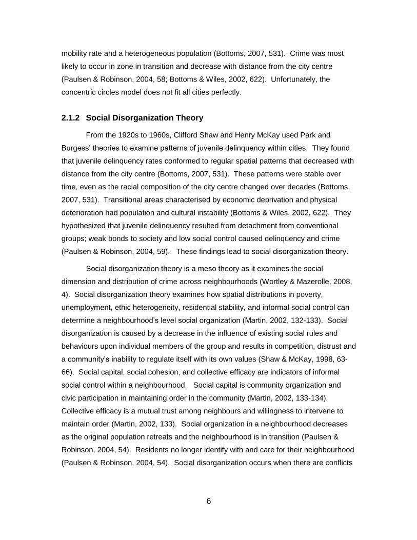
Figure 1 below depicts the awareness space consisting of the individual’s paths
and nodes (Brantingham & Brantingham, 1981, 37; Bottoms & Wiles, 2002, 639). This
diagram shows the areas immediately surrounding an offender’s nodes, where targets
are present, is where crime opportunities present themselves and crime is likely to occur
(Brantingham & Brantingham, 1993a, 10; Brantingham & Brantingham ,1984, 353). This
includes areas where a person travels and a person’s knowledge of the surrounding
areas close to those areas (Brantingham & Brantingham, 1984, 352). Potential victims
and offenders have similar activity patterns within the same environment; therefore, they
share activity nodes and pathways (Andresen, 2010, 20). According to Brantingham and
Brantingham, the convergence of an offender’s and victim’s activity and awareness
spaces leads to the occurrence of crime (as cited in Frank et al., 2012, 181).

14
Figure 1. Brantingham’s diagram of nodes, paths, activity space, and awareness space
People are familiar with some areas of the city more than others; these areas
tend to be places near our homes, where we work, go to school or go for shopping and
entertainment and the roads between them (Bottoms & Wiles, 2002, 638). Other areas
we are not familiar and tend not to frequent (Bottoms & Wiles, 2002, 638). As offenders
establishes daily patterns of behaviour and activity spaces, they become more familiar
with certain areas and develop awareness spaces from which they are more likely to
come across opportunities for crime and select targets (Brantingham & Brantingham,
1993a, 10). Most offenders will commit crimes in areas they are familiar. As discussed
above, the activity space consists of the nodes and paths that we frequent and our
activity space is the familiar area surrounding theses nodes and paths.
Different neighbourhoods have different populations with different socio-
demographic and socio-economic characteristics (Andresen, 2006b, 491). These
different characteristics within a neighbourhood, along with the presence of activity
nodes, influence the routine activities of the population within the area (Andresen,
2006b, 491). They also influence the number of motivated offenders, availability of
suitable targets and the presence of capable guardians in the area (Andresen, 2006b,
491). For example, the population size and the number of dwellings in a neighbourhood
can influence the number of potential targets, while the average value of dwellings and

15
average family income can influence the suitability of those targets (Andresen, 2006b,
491; Andresen, 2006c, 261). The percentage of young males in the population can
influence the number of potential offenders in a neighbourhood, while the unemployment
rate can influence the motivation of potential offenders (Andresen, 2006b, 491). Finally,
composition of households in a neighbourhood, including single marital status, lone
parents and female-headed households, can influence the presence of capable
guardians.
2.1.5 Crime Pattern Theory
In the 1990s, Patricia and Paul Brantingham (1993) used concepts from routine
activity theory, rational choice theory, the geometric theory of crime, along with
opportunity theory, and lifestyle exposure theory, to create crime pattern theory. Routine
activity theory examines variations in the social environment that lead to crime
(Andresen, 2010, 27). Rational choice theory examines the cognitive environment that
influences the decision to commit crime (Andresen, 2010, 27). The geometric theory of
crime examines the built environments influence on crime (Andresen, 2010, 27). Crime
pattern theory is a meta-theory that uses the common concepts from these
environmental criminology theories and the concepts of crime templates and
environmental cues to understand how criminals select targets within their routine
activities and within the legal, psychological, social and physical environment (Andresen,
2010, 26-27). It examines the influence of the physical and social environment on the
distribution of crime events over time and space and the way targets come to the
attention of offenders (Eck & Weisburd, 1995, 6). Crime pattern theory focuses on the
non-uniformity and non-randomness of the criminal event (Wortley & Mazerolle, 2008,
12). Crime occurs at predictable locations where criminal opportunity and an offender’s
awareness space coincides (Wortley & Mazerolle, 2008, 12).
According to Brantingham and Brantingham, crime is an event in which a
motivated offender decides to commit a crime and locates a potential target within their
awareness space (Brantingham & Brantingham, 1993b, 261). “Each element in the
criminal event has a trajectory shaped by past experience and future intention, by the
routine activites and rhythms of life, and by the constraints of the environment”
(Brantingham & Brantingham, 2008, 78). As individuals move through their daily
activities, they make decisions that become routine and create a template that guides

16
their behaviour (Brantingham & Brantingham, 2008, 80). As potential offenders move
about between nodes such as home, work, leisure, school, and shopping they take
paths that become routine; these spatial and temporal movement patterns constrain their
activity and create an awareness space in which the offender is familiar and becomes
aware of suitable targets (Brantingham & Brantingham, 2008, 83-85). Opportunities for
crime are developed by the routine activities of daily life; crime will occur where the
potential target and offender’s activity spaces or pathways overlap (Brantingham &
Brantingham, 2008, 87).
There are seven propositions in crime pattern theory. First, some individuals are
motivated to commit specific offences, and this motivation varies by person
(Brantingham & Brantingham, 1978, 107). Second, the commission of an offence is the
result of a multi-staged decision process in which an offender locates a target within the
environment in time and space (Brantingham & Brantingham, 1978, 107). Third, the
environment emits cues about the spatial, cultural, legal and psychological
characteristics of an area (Brantingham & Brantingham, 1978, 107). Fourth, motivated
offenders use these environmental cues to identify targets (Brantingham & Brantingham,
1978, 107). Fifth, motivated offenders learn which cues are associated with good
targets by experience, developing crime templates and search patterns (Brantingham &
Brantingham, 1978, 108). Sixth, once a template is established it becomes fixed and
self-reinforcing, influencing future behaviour (Brantingham & Brantingham, 1978, 108).
Finally, there can be many potential crime templates but these are limited (Brantingham
& Brantingham, 1978, 108).
Criminal events begin with a rational decision process in which an offender is in a
state of readiness to commit a crime and has motivation and knowledge to carry out the
crime (Brantingham & Brantingham, 1993b, 261). People make decisions as they move
through activities and as these activities are repeated, they develop templates
(Brantingham & Brantingham, 2008, 80). These templates can be adapted to overcome
factors and modified for the situation (Brantingham & Brantingham, 2008, 83). Potential
offenders make rational choices of whether or not to commit crimes (Andresen, 2010,
27). The number and sequence of decisions made by the offender varies by the type of
crime (Brantingham & Brantingham, 1993b, 262). The level of readiness depends on
the individual, the situation, the environment and the availability of opportunities and
varies over time (Brantingham & Brantingham, 1993b, 262). The suitability of a target is

17
a function of the characteristics of the target and its surroundings (Paulsen & Robinson,
2004, 108). Offenders determine whether a potential target or crime site is suitable in a
decision process based on factors such as the characteristics of the target, the
characteristics of the offender, the characteristics of the crime site, the characteristics of
the immediate situation, and the characteristics of the backcloth (Brantingham &
Brantingham, 1993b, 263-264).
The environmental backcloth consists of the elements surrounding an individual
that influence their behaviour through their reaction to cues emitted from their
surroundings (Brantingham & Brantingham, 1993b, 264). The environmental backcloth
is formed from routine activities and creates a template from which an offender can
identify good and bad opportunities for crime (Brantingham & Brantingham, 1993b, 268).
Backcloths are non-static and have many dimensions including social, cultural,
economic, legal, structural, spatial, temporal and physical dimensions, which are
constantly changing (Brantingham & Brantingham, 1993b, 265). Elements of a
backcloth include the street network, land use, socio-economic status of residents,
transit system, and type of housing of an area (Brantingham & Brantingham, 2008, 87).
Crime has a strong correlation with the physical features of the environment, such as the
type and location of buildings, street parks, automobiles, and highways (Harries, 1980,
93). Different elements of the backcloth may trigger crime for different people
(Brantingham & Brantingham, 1993b, 281).
The characteristics of a place influence the likelihood of crime occurring.
Facilities provide reasons for people to go to different places within the city to carry out
their lifestyles and can be the point of where victims and offenders meet in the absence
of handlers and guardians (Roncek & Maier, 1991, 727). Facilities such as schools,
taverns, convenience stores, apartment buildings and public housing, all influence the
amount of crime in the immediate environment through the dispersion of targets, their
attraction to potential offenders and the amount of control place managers and
guardians have over the site (Eck & Weisburd, 1995, 8-9). Some geographic areas
have more crime than others as crimes tend to cluster or re-occur at certain locations
due to the social structure of places (Eck & Weisburd, 1995, 12). Site features, such as
surveillance, territoriality, guardianship, place management, target hardening and
decreasing target attractiveness decrease the amount of crime in one place by making it
harder and less inviting for criminals to commit crimes (Eck & Weisburd, 1995, 13-16).

18
Crime generators are places with a high flow of people (both potential offenders
and targets) through and to nodal activity area for reasons unrelated to crime, such as
shopping or entertainment districts or sporting events; providing a time and place for
crime opportunities (Brantingham & Brantingham, 2008, 89). Crime generators are
places that attract large numbers of offenders and victims due to the nature of activity
that can lead to a larger number of criminal incidents because of the volume of people in
the area (Lersch, 2007, 205-206). Crime generating areas have particular times and
places that provide enough people and targets in a setting conducive to particular types
of crime (Brantingham & Brantigham, 2008, 89). Local and outside offenders do not
come to these areas with the intent to commit crime, however, motivated offenders may
end up committing crime at these areas as the opportunity presents itself (Brantingham
& Brantigham, 2008, 89).
As these areas well known to motivated offenders as areas that create criminal
opportunity for particular types of crime, they become crime attractors (Brantingham &
Brantigham, 2008, 89). Crime attractors are areas that are known to provide many
criminal opportunities and draw motivated offenders to the location to locate targets and
commit crime, such as bar districts, and major transit exchanges (Brantingham &
Brantingham, 2008, 89; Lersch, 2007, 204). Crime attractors can also include illegal
businesses for gambling, fencing, prostitution, and drug dealing (Bernasco & Block,
2011, 35). Crime attractors and generators can become hot spots as they bring together
potential victims and offenders (Brantingham & Brantingham, 2008, 89). Brantingham
and Brantingham note that most crimes are committed by young people, therefore,
identifying attractors and nodes popular with young people helps to identify where
crimes occur (Brantingham & Brantingham, 1993a, 17).
Hot spots are predicted by taking into consideration the convergence elements of
the crime event discussed by crime pattern theory (Brantingham & Brantigham, 2008,
90). The residential and activity locations of potential offender populations, the spatial
and temporal distribution of potential crime targets and capable guardians, the activity
structures of the city including activity nodes and land uses, the transportation networks
and flow of people throughout the city, and the underlying social and physical
environment all influence the occurrence of crime and hot spots in a city (Brantingham &
Brantingham, 2008, 90). The clustering of crime in a city is shaped by the people who
live within the city and how they move about the city and spend their time (Brantingham

19
& Brantingham, 2008, 91). The overlap of activity nodes of potential offenders and
targets can create crime generators and crime attractors which can be identified as hot
spots (Brantingham & Brantingham, 2008, 91).
Hot spots are areas associated with a high risk of victimization and
proportionately greater number of criminal incidents than other areas (Anselin, Griffiths &
Tita, 2008, 99). They are a concentration or cluster of crimes in space (Lersch, 2007,
203). Studies have found that a small number of specific locations within a city generate
the majority of reported crime (Bottoms & Wiles, 2002, 628). “Most police calls for
service come from especially dangerous locations, or hot spots”; the worst 10% of
places account for 30% of all calls for service (Spelman, 1995, 115; 142). Hot spots are
smaller than neighbourhoods and are comprised of blocks or street segments that
experience high levels of crime (Anselin, Griffiths & Tita, 2008, 99).
Some hot spots are not high crime areas all the time; they may vary by time
(Lersch, 2007, 204). For example, shopping malls are only open certain hours of the
day, universities have classes a certain times during the day and sporting events on the
weekends, entertainment districts are mainly visited on weekend and evenings and
central business districts are busiest on week days (Lersch, 2007, 251). The space-time
path is a person’s movement through time and space as they travel through their daily
activities (Lersch, 2007, 251). There are time constraints that limit people’s movements
and opportunities to travel to events and participate in activities (Lersch, 2007, 251).
Temporal analysis of crime patterns by seasons, months, day of the week, weekday
versus weekends and time of day are useful to identify natural fluctuations in crime
levels (Getis et al., 2000, 10).
By mapping the home and activity locations of offender, targets and guardians in
time and space, the residential and activity structures of the city, land uses, and the
structure of transportation networks we can predict the areas where crime is most likely
to occur (Brantingham & Brantigham, 2008, 90). Crime mapping is useful in illustrating
the concepts of crime pattern theory; nodes, paths, edges, and activity spaces can be
mapped to demonstrate site selection (Paulsen & Robinson, 2004, 111).
2.1.6 GIS and Crime Mapping
In the 1990s, geographic information systems (GIS) mapping technology
furthered the modelling of spatial and temporal distributions in crimes and the

20
identification of hot spots (Wortley & Mazerolle, 2008, 12). GIS uses computers to
displays maps of crime locations, along with environmental features and area
boundaries, and shows the spatial relationships associated with crime data (Canter,
1998, 160). Crime mapping provides “a better understanding of the environmental
factors that influence criminal behaviour” (Canter, 1998, 174).
GIS displays and analyzes the location of crime and other dimensions of the
criminal event, such as offenders, targets and the environmental backcloth (Canter,
1998, 161). GIS quickly maps large amounts of data into crime locations and displays
the intensity of crime in an area over time and space in relation to attributes associated
with the crime and geography (Canter, 1998, 164-165). GIS delineates the boundaries
of neighbourhoods into geographical units to help understand the crime differences
between, within, and across neighbourhoods (Wilson, 2009, 1). Datasets can be
geocoded to show the effects of population groups on offence rates (Bottoms & Wiles,
2002, 624). Street networks, land uses, locations of schools, other geographical
features and census information are to test hypotheses about the relationship between
crime and physical and land use features (Canter, 1998, 168; Dunn, 1980a, 5).
From the development of GIS has emerged geographic profiling and intelligence
led policing. Geographic profiling uses the principles of environmental criminology to
map crime data and predict where a criminal is most likely to live. Crime patterns and
trends help police understand criminal behaviour and target resources more effectively.
GIS can be used to predict police response times, crime displacement, and demand for
police services (Canter, 1998, 171). GIS is also used to create policy and develop crime
prevention initiatives.

21
3. Literature Review
3.1. The City of Ottawa
The environmental characteristics of the City of Ottawa are important to the
spatial analysis of crime patterns, as certain the features of the environment can
influence behaviour and in turn increase the likelihood of crime. The physical features of
a city can include the location of central business districts, industrial and residential land
uses, street networks, and rivers. The social features of a city can include socio-
demographic and socio-economic characteristics of the residents. These features
become a part of the environmental backcloth and can influence people’s behaviours
including their awareness spaces and travel patterns and the concentration of people
throughout a city.
The City of Ottawa is located in southeastern Ontario, on the border between the
provinces of Ontario and Quebec, on the Ottawa River. Across the river from Ottawa is
the city of Gatineau, Quebec. Ottawa is located 352 km east of Toronto and 192 km
west of Montreal (Ottawa Tourism, 2010, 10). Ottawa has the Rideau Canal, a national
historic site and landmark, located in the downtown area. Ottawa is the fourth most
populated city in Canada, with a population of 812,130 (Community Foundation of
Ottawa, 2007, 4). The median age of the population in 2006 was 38.4 years. The
majority of Ottawa’s workforce is in the service sector (88%), and the government is the
largest employer (Community Foundation of Ottawa, 2007, 4-5). The majority of people
in Ottawa drive cars for transportation (58%); only 13% of the population takes public
transportation (Community Foundation of Ottawa, 2007, 22). Ottawa has rural villages,
farms, and hamlets surrounding the city centre and suburbs. The outlying population
has been growing faster than the city as people move away from the city core
(Community Foundation of Ottawa, 2007, 5).
Ottawa’s parliament buildings are located on Wellington Street in the downtown
area (Ottawa Tourism, 2010, 28). The Governor General’s Rideau Hall is located at 1
Sussex Drive, also in downtown Ottawa (Ottawa Tourism, 2010, 28). Ottawa’s central
business district is located in the downtown core near the river. Ottawa has several

22
entertainment areas, most of which are located in or near the downtown core. Ottawa’s
Chinatown, a multicultural village with Asian dining, shopping, and entertainment, is also
located downtown (Ottawa Tourism, 2010, 51). Downtown Rideau, Ottawa’s city centre
with shopping, restaurants, theatres, and cultural activities, is located downtown east of
the Rideau Canal (Ottawa Tourism, 2010, 51). Preston Street, or “Little Italy”, offers
restaurants and specialty stores and Sparks Street, Canada’s first pedestrian mall and
commercial area, are also located in downtown Ottawa (Ottawa Tourism, 2010, 51).
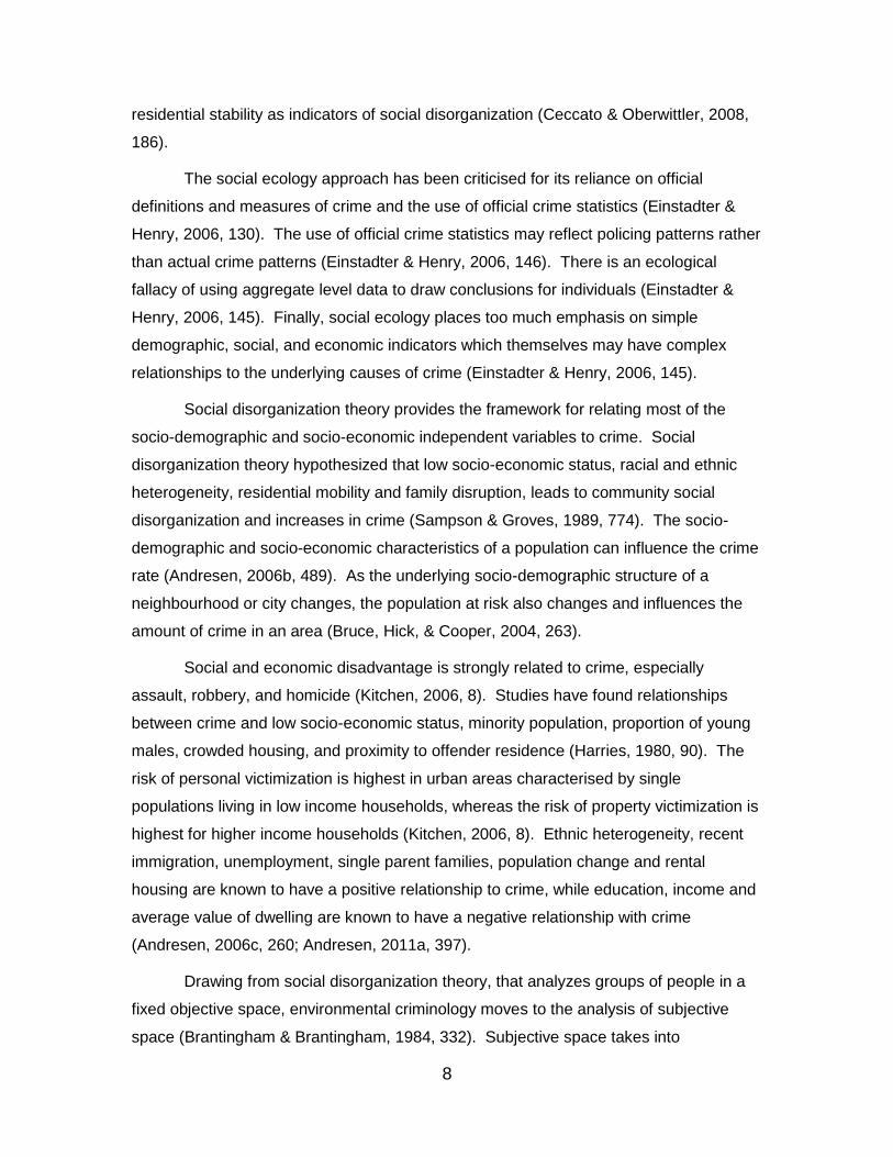
Figure 2 below shows the downtown area of Ottawa in relation to the two universities.
Figure 2. Map of downtown Ottawa and the universities
Ottawa has two major universities, the University of Ottawa and Carleton
University. The University of Ottawa is located in downtown Ottawa at 550 Cumberland
Street, between Laurier and Mann Avenue and between King Edward Ave and Nicholas
Street, near the Rideau Canal. The University of Ottawa is also located near the By
Ward Market, Parliament Hill and the downtown centre areas of the city. The University
of Ottawa was established in 1848 and is the largest bilingual university in North
America (University of Ottawa, 2011). Maclean’s magazine classifies the University of

23
Ottawa as a medical/doctoral university (Dwyer, 2006). The University of Ottawa has a
population of approximately 40,000 students, teaching and support staff, with residences
that can hold approximately 2,800 students (University of Ottawa, 2011). The University
of Ottawa has off-campus facilities located throughout Ottawa, including the Alta Vista
campus located in the Riverview neighbourhood of Ottawa on Smyth Road and the
Centre for Executive Leadership at the World Exchange Plaza located in downtown
Ottawa on O’Connor Street.
Carleton University is located just south of downtown Ottawa at 1125 Colonel
ByDrive, between Dow Lake, the Rideau River, and Bronson Drive. In addition to the
lake, river and canal, three parks, Brewer Park, Vincent Massey Park, and Fletcher
Wildlife Garden surround the campus. Carleton University was established in 1942
(Carleton University, 2011). Maclean’s magazine classifies Carleton University as a
comprehensive university (Dwyer, 2006). Carleton University has a population of
approximately 25,000 students, teaching and support staff with residences that can hold
approximately 2,800 students (Carleton University, 2011). The buildings at Carleton
University are connected via an underground tunnel system so students do not need to
walk outside to move around campus.
In 2006, Ottawa had a median income of $80,300, more than the provincial
median income of $64,500 and national income of $60,600 (Community Foundation of
Ottawa, 2007, 4) Ottawa’s median income has increased by 17% since 2000
(Community Foundation of Ottawa, 2007, 4). Nineteen percent of Ottawa’s families lived
below the poverty line, less than both the Ontario and Canada overall (Community
Foundation of Ottawa, 2007, 7). Ottawa’s unemployment rate in 2006 was 5.1%, well
below the national and provincial levels (Community Foundation of Ottawa, 2007, 20).
Ottawa’s wealthiest neighbourhood is Rockcliffe Park that had an average income of
$225,035 in 2000; this was six times the average income of Vanier, Ottawa’s poorest
neighbourhood at $36, 312 (Community Foundation of Ottawa, 2007, 7). The average
house price in 2006 was $257,418, a 3.7% increase from 2005 (Community Foundation
of Ottawa, 2007, 15).
There is a growing gap between the rich and poor in Ottawa, that is increasing
Ottawa’s homeless population (Janhevich, Johnson, Vezina, & Fraser, 2008, 37). In
2006, 23,160 social housing units were available but 10,055 households were still on the
waiting list (Community Foundation of Ottawa, 2007, 15). The number of people

24
accessing emergency shelters increased by 2% from 2005 (Community Foundation of
Ottawa, 2007, 15). There is also a growing crack cocaine problem in Ottawa’s city
centre (Janhevich et al., 2008, 37). Since 1982, Ottawa has implemented various crime
prevention strategies and attempted to build relationships between the police and other
community agencies (Janhevich et al., 2008, 38).
Ottawa has one of the lowest crime rates in Canada and the crime rate has
remained stable since 1999, with a slight decrease in 2002 (Kitchen, 2006, 13-15). In
2006, Ottawa census metropolitan area (CMA) had an overall crime rate of 5,775 per
100,000 population, a violent crime rate of 580 per 100,000 population, and a property
crime rate of 3,075 per 100,000 population (Community Foundation of Ottawa, 2007, 8).
This overall crime rate in Ottawa CMA decreased from 6,326 offences per 100,000
population in 2003 (Andresen & Linning, 2012, 276). Property crime and violent crime in
Ottawa decreased by 34% and 22% respectively from 2000 to 2006, although the
perception of crime increased (Community Foundation of Ottawa, 2007, 8). According to
Statistics Canada, Ottawa CMA had a robbery rate of 92 offences per 100,000, a
burglary rate of 550 offences per 100,000, and a motor vehicle theft rate of 327 offences
per 100,000 in 2006 (Silver, 2007, 13).
In comparison, Canada’s crime rate has decreased since the1990s with a slight
increase in 2003 (Bunge, Johnson, & Balde, 2005, 8). Canada had an overall crime rate
of 7,500 per 100,000 in 2006, a violent crime rate of 951 per 100,000 and a property
crime rate of 3,587 per 100,000 (Statistics Canada, 2008, 80). Ottawa CMA's overall
crime rate in 2006 was slightly greater than that of Toronto CMA (5,020 offences per
100,000 population), slightly lower than that of Montreal CMA (6,912 offences per
100,000 population), and nearly half the overall crime rate of Vancouver CMA (10,609
offences per 100,000 population) (Andresen & Linning, 2012, 276).
A study conducted by Kitchen (2006) of the Department of Justice Canada,
examined crime in relation to demographics and social status in Ottawa. This study
examined 2001 crime data from the Ottawa Police Service and socio-economic
indicators from the 2001 Census data aggregated at the dissemination area (Kitchen,
2006, 22). The study used six groups of offences (rate per 1,000 population) as the
dependent variables: total offences, violent offences, major property offences, minor
property offences, drug offences and disturbances/other offences (Kitchen, 2006, 22).
Twenty six socio-economic variables were used as the independent variables including:

25
unemployment, labour force participation, low income, low education, recent immigrants,
visible minorities, lone parent families, marriage status, residents who had moved in past
year, owned or rented dwellings, age of housing, type of housing and household density
(Kitchen, 2006, 23). The study hypothesized that there was a positive relationship
between crime and disadvantaged communities in Ottawa (Kitchen, 2006, 7).
Kitchen used principal components analysis to examine the relationship between
the types of crime and the socio-economic variables, as well as standard and step-wise
multiple regression models to identify the significant predictors of crime and the strength
of the relationship (Kitchen, 2006, 33-34). The study also used ArcGIS and choropleth
maps to analyze the spatial relationship of crime in Ottawa (Kitchen, 2006, 34). Overall,
the study found a weak association between crime and the socio-economic variables in
Ottawa and there were no clear predictors of crime at the dissemination area level
(Kitchen, 2006, 37). No more than 11% of the variance was explained for any of the
crime types by the socio-economic variables (Kitchen, 2006, 38). However, the study
did find higher crime rates in areas characterised by residential mobility and people living
in low income households (Kitchen, 2006, 38).
High crime areas in Ottawa were concentrated in the central core and suburbs,
while fewer crimes were in the outer, rural areas of the city (Kitchen, 2006, 39). The
highest crime levels were found in the downtown central business district and Market
area, as well as the east-central Vanier, Overbrook, and Ottawa North-East areas and
several communities west of downtown in Carlington (Kitchen, 2006, 39). These areas
had mostly minor property crimes such as theft under $5000 and theft from vehicles
(Kitchen, 2006, 39). The Market area had higher than average violent crime, especially
for theft and assault (Kitchen, 2006, 39). There were also corridors of crime found along
major the transportation routes: Highway 417, Highway 17, and Highway 16 (Kitchen,
2006, 39). Hot spots of crime and disadvantage were found in Ottawa’s central core,
especially in the inner city neighbourhoods of Dalhousie, Centre Town, Sandy Hill, and
Lower Town (Kitchen, 2006, 41). Larger clusters of crime and disadvantage were found
in the east-central areas of Vanier, Overbrook, and Ottawa-North East, as well as the
suburban communities of Riverview, Alta-Vista, Hunt Club, Pinecrest- Queensway, and
Nepean North (Kitchen, 2006, 41). The author also aggregated the data to the
neighbourhood level of analysis and found that the strength of the statistical relationship
increased for several indicators (Kitchen, 2006, 85).

26
Kitchen (2006) found some support for social disorganization theory as there
were hot spots of violent crime with significantly larger proportions of recent immigrants,
visible minorities and residents living in apartment buildings (Kitchen, 2006, 43).
However, 60% of the high crime areas in Ottawa were not socially disadvantaged
(Kitchen, 2006, 43). These areas had suitable targets in commercial, institutional, and
recreational areas where shopping centres, offices, transit stations, warehouses and
recreation centres were located (Kitchen, 2006, 43). Unguarded homes in suburban
communities made suitable targets for theft and the high concentration of bars and
restaurants in the Market area had high levels of violent crime (Kitchen, 2006, 43).
These findings supported for routine activity theory.
3.2. Universities and Crime
Certain places, locations, and areas have a disproportionately high risk for
certain types of crime (Block & Block, 1995, 147). Some places have characteristics that
generate or attract certain types of crime (Block & Block, 1995, 147). “The aggregate
distribution of crime seems to be substantially related to the socio-economic and socio-
demographic mosaic of cities as well as the location of major population attractors”
(Brantingham & Brantingham, 1993a, 5). Nodes vary in risk of crime according to the
characteristics of the surrounding environmental and situational factors (Block & Block,
2000, 137). Some major population attractors can include entertainment and central
business districts, shopping centres, and even university campuses.
The crime pattern theory, including geometric theory of crime, provides the
framework for relating the independent variables, the two universities, to crime. As
discussed previously, these theories examine the convergence of a motivated offender,
a suitable target and lack of a capable guardian in time and space. It is within the
routine activities of travelling from work, home, school, and entertainment that these
elements meet and the opportunity for a criminal event presents itself. The nodes, paths
and edges within a person’s activity space influence their travel patterns and awareness
space. Potential offenders use environmental cues from within their awareness space to
identify suitable targets and make decisions to commit crime. If an area has suitable
targets and a lack of capable guardians it can become a crime generator for offenders.
As offenders frequent the area and successfully commit crimes, they develop crime
templates for committing future offences, and the area can become a crime attractor.

27
Universities are activity nodes where students, staff and other members of the
public come together in the course of their routine activities. Universities bring a large
number of people to the campus for school or work during the day. Universities may
also bringing young people to the campus for entertainment such as sporting events,
drinking and partying in the evening. Most campuses have residences where students
live, many away from home for the first time. These factors all bring large numbers of
people together including potential offenders, targets and lack of guardians together,
creating potential crime opportunities. Universities can provide suitable targets in the
absence of capable guardians. Universities have a concentration students living alone
or visiting the campus who own laptops and other goods that are attractive to burglars
and robbers. Universities also have large parking lots for students and staff to park their
vehicles while they attend class that provide opportunities for motor vehicle theft. As
people travel to the university and become familiar with the area, the university becomes
a part of their awareness space. As many people frequent campuses daily, universities
make up a part of many people’s awareness spaces. Universities have environmental
characteristics favourable to crime that influence a potential offender’s decision to
commit crime, including the presence of large numbers of young people on campus,
large transportation centres, and mixed commercial and residential land use. These
characteristics of universities can provide opportunities for crime on campus and result
in universities becoming crime generators and even crime attractors.
A number of studies have examined the factors influencing crime on university
campuses. Some studies have found that campuses have lower crime rates than the
general population (Henson & Stone, 1999, 302; Volkwein et al., 1995, 657). University
crime is associated with the percentage of students living in dormitories, the
unemployment rate, and the security expenditures of the school (McPheters, 1978, 49).
McPheters (1978) found a positive relationship between security expenditures and crime
that is contrary to routine activity theory’s premise of guardianship. However, this finding
may due to the detecting and reporting rates of crime rather than security activity
(McPheters, 1978, 50). The positive relationship between dormitory population and
crime may be due to the larger number of potential targets at a residential campus in
comparison to a commuter campus (McPheters, 1978, 50). Studies of crime at campus
residences have found that 70% of the crimes occurred between midnight and 7:00am
(Molumby, 1976, 250). Larger residence buildings, residences located along major
routes, and residences with poor visibility and surveillance have a disproportionate

28
amount of crime (Molumby, 1976, 256-257). The positive relationship between the
unemployment rate off-campus and the crime rate on campus might be attributable to
the motivated offenders travelling to campuses in search of potential targets (McPheters,
1978, 50). Malczewski and Poetz (2005) found hot spots of burglary in the areas
adjacent to the University of Western Ontario; these areas were characterised by large
proportions of rental accommodations and young transient populations, as is the case
for most university students (Malczewski & Poetz, 2005, 518).
Brower and Carroll (2007) examined the patterns of alcohol related crime at the
University of Wisconsin and student and non-student neighbourhoods in Madison,
Wisconsin. They used ArcView 3.3 to map 12,772 calls for service, including liquor law
violations, assaults, vandalism, and noise complaints in 2003, and the proximity of
student and non-student neighbourhoods to high-density bar areas (Browser & Carroll,
2007, 268). The student address data was obtained from the University of Wisconsin’s
office of the registrar for the spring 2003 semester, including undergraduate, graduate
and part-time students in order to determine high-density student neighbourhoods
(Browser & Carroll, 2007, 268). The authors focused on the downtown area of the city
near the university as this area included the majority of the student residences and high-
density bar areas (Browser & Carroll, 2007, 269).
The authors found that crimes were not distributed evenly throughout the city or
throughout the day (Browser & Carroll, 2007, 269). Noise complaints increased steadily
from 6:00pm until the peak at 11:00pm, while assaults increased from 11:00pm until the
peak at 2:00am when the bars closed (Browser & Carroll, 2007, 269-271). Noise
complaints were highest in the areas bordering between student and long-term resident
neighbourhoods around 10:00pm when long-term residents would be going to sleep
(Browser & Carroll, 2007, 271). Noise complaints increased again from 2:00am to
3:00am in the high-density bar areas where other crimes, such as assaults were
occurring when the bars closed (Browser & Carroll, 2007, 271). Vandalism followed
different patterns than the other types of crimes; vandalism peaked from 8:00am to
10:00am and again at 3:00pm in the high-density student neighbourhoods (Browser &
Carroll, 2007, 271). This study showed that university high-density student
neighbourhoods are related to some crime problems due to student drinking (Browser &
Carroll, 2007, 273).

29
Volkwein, Szelest and Lizotte (1995) examined the relationship between campus
crime and campus and student characteristics at 416 American post-secondary
institutions. The authors used structural/functional perspectives from organizational
literature as their theoretical framework to examine the influence of campus’
organizational goals, size, wealth, complexity, technology, and environment on the
behaviour and values of students (Volkwein et al., 1995, 648-649). They also used
routine activity theory to examine the convergence of likely offenders, suitable targets,
and absence of capable guardians in time and space within the campus community
(Volkwein et al., 1995, 649). The authors hypothesized that campuses were more likely
to attract crime than to generate crime, as offenders were more likely to live off campus
than on campus (Volkwein et al., 1995, 661). The authors used crime data from the FBI
Uniform Crime Report (UCR) from 1974 to 1991 to examine the change in crime trends
at campuses over time (Volkwein et al., 1995, 651). They also used crime data from the
1990 FBI UCR database, the Consortium for Higher Education Campus Crime Research
datasets, and information on campus and student characteristics from the Integrated
Post-secondary Education Database System and the College Board Survey (Volkwein et
al., 1995, 651).
The longitudinal analysis of crime data which compared national to campus crime
rates from 1974 to 1992 showed that campuses are over ten times safer than the nation
in general (Volkwein et al., 1995, 657). While violent crime was increasing in the nation
in general, it was decreasing on campuses (Volkwein et al., 1995, 657). Property crime
on campus followed similar patterns to the nation in general until 1985 when property
crime began to decrease on campuses and increase in the nation in general (Volkwein
et al., 1995, 657). The authors found significant differences in crime trends by campus
type with the lowest violent and property crimes found at two-year institutions, which
were mostly non-residential (Volkwein et al., 1995, 659). The highest rates of property
crime were found at medical schools and health science institutions with affluent
personnel, expensive equipment, inner city clientele and a small student body (Volkwein
et al., 1995, 659). Crime rates on campuses were six to ten times safer from violent
crime when compared to crime rates in the communities in which they were located
(Volkwein et al., 1995, 660). Assaults were found to the most frequent type of violent
crime and larceny was the most frequent type of property crime both on and off campus
(Volkwein et al., 1995, 660). Burglary and motor vehicle theft rates were found to be
very low at all types of institutions (Volkwein et al., 1995, 660).

30
The multiple hierarchical regression showed the student characterstics, including
selectivity, diversity, and transfers, explained the greatest amount of the variance for
violent crime (Volkwein et al., 1995, 661). Campus organizational characteristics,
including wealth, size, cost, and complexity, explained the greatest amount of the
variance for property crime (Volkwein et al., 1995, 661). Community characteristics,
including crime rates, population and poverty, by themselves, did not explain significant
amounts of the variance in any of the three crime types (Volkwein et al., 1995, 661). All
23 of the independent variables explained 79% of the variance in property crime and
less than one third of the variance in violent crime (Volkwein et al., 1995, 661). A
stepwise regression using violent crime as the dependent variable showed that
campuses with the highest rates of violent crime had higher than average percentages
of African American students and higher than average resources for student revenues
and library holdings (Volkwein et al., 1995, 661-662). The stepwise regression for
property crime showed several campus organizational characteristics (especially student
revenue, room and board, library holdings, and campus police per capita) and a few
student characteristics were associated with campus property crime (Volkwein et al.,
1995, 662). Public colleges and universities had more property crimes than private
institutions when controlling for all other variables (Volkwein et al., 1995, 662).
Bromley (1995) examined the influence of security features and demographic
and campus characteristics on crime in college and university campuses (Bromley,
1995, 14). The author examined campus crime data from the International Association
of Campus Law Enforcement Administration for 265 American colleges and universities
(Bromley, 1995, 15). The author also used data on campus security, campus and
demographic characteristics from the 1992 Barrons Profile of American Colleges
(Bromley, 1995, 15). Demographic variables included student population, number of
male students and number of female students, undergraduate student age, number of
non-white students, number of students living in dorms, number of buildings on campus,
number of campus acres, and number of index crimes (Bromley, 1995, 15). Campus
characteristics variables included small, urban, rural, or suburban town, whether or not
there was a large coliseum or football stadium on campus, and level of security
(Bromley, 1995, 15).
The author examined the correlations between the independent variables and
overall number of campus crimes and found that several variables were significantly

31
related to crime including student population, number of male and female students,
number of non-white students, number of students living in dormitories, and number of
buildings on campus (Bromley, 1995, 15). The author conducted a series of one-way
analyses of variance (ANOVA) tests to determine if the independent variables were
associated with the number of crimes on campus (Bromley, 1995, 15). There were
significant differences found for the type of institution, the presence of a stadium, and the
level of security (Bromley, 1995, 15). Forward stepwise regression results showed that
number of dormitory students was the strongest predictor of campus crime accounting
for 66% of the variance, followed by number of acres that explained an additional 4% of
the variance (Bromley, 1995, 15). Overall, it was found that large student populations
and the number of dormitory students were associated with campus crime as these
campuses had a larger number of potential targets (Bromley, 1995, 16). Number of
acres and number of buildings were also associated with campus crime (Bromley, 1995,
16). In agreement with other studies, the author also found that a greater level of
security was associated with crime (Bromley, 1995, 16). This may be due to campuses
increasing security programs in response to crime problems (Bromley, 1995, 16).
Fox and Hellman (1985) examined the effect of various characteristics of
campuses, such as location, campus size and scholastic quality, on the amount of crime
in 22 American colleges and universities to determine if campuses are relatively safer
than the surrounding cities (Fox & Hellman, 1985, 429-430). Universities have a
relatively homogeneous population based on characteristics such as age, education,
and residential mobility (Fox & Hellman, 1985, 429). University campuses can attract or
repel criminal activity from the surrounding community (Fox & Hellman, 1985, 430). The
authors reviewed the crime rates for 176 campuses in comparison to the city or towns in
which they were located as a ratio of campus to city (Fox & Hellman, 1985, 431). They
found higher ratios of campus to city crime rates in rural communities and lower campus
to city crime rate ratios in urban areas (Fox & Hellman, 1985, 431). The authors also
found that location of a campus (urban, rural, and suburban) had no association with the
campus crime rate, therefore campus overall crime rates was not affected by the
environment of the city in which they are located (Fox & Hellman, 1985, 433-434).
The authors examined characteristics of campuses including police and security
measures, finances, student and building density, accessibility and visibility, community
and cohesiveness, scholastics, student body demographics, and location characteristics

32
(Fox & Hellman, 1985, 435-436). The authors conducted principal components analysis
with the campus crime rates (Fox & Hellman, 1985, 440). They found that campus
location including the distance from city centre, unemployment rate, and population of
city had no effect on campus crime rates (Fox & Hellman, 1985, 440). The authors did
find however, that higher police enforcement was associated with higher crime rates,
and scholastic quality and campus size had a strong positive effect on campus crime
rates (Fox & Hellman, 1985, 439-441).
Sloan (1994) extended studies conducted by McPheters and Fox and Hellman to
examine factors influencing crime at 481 American college and university campuses by
(Sloan, 1994, 54). Sloan used secondary data on offences know to campus police or
security for American campuses between 1989 and 1990 (Sloan, 1994, 52-53). The
crimes included total offence, theft and burglary offences, violent offences, vandalism
offences, and assaults (Sloan, 1994, 53). The author also examined crime prevention
measures used at the campuses and campus characteristics such as number of full-time
faculty, number of students and faculty members per acre, a ratio of students to faculty,
and the number of fraternities and sororities located on campus (Sloan, 1994, 53).
There were 195,000 offences reported on the campuses from 1989 to 1990;
most of these offences were burglary or theft offences (64%) and only 6% were violent
offences (Sloan, 1994, 54). Vandalism accounted for 19% of offences and drinking and
drug related offences accounted for 11% of offences on campus (Sloan, 1994, 54). The
author used principal components factor analysis to identify seven discrete factors
associated with crime on campuses (Sloan, 1994, 56). The factors included size,
academics, students, crowding, safety, minorities, and setting (Sloan, 1994, 56).
Multiple regression was then used with these factors (Sloan, 1994, 56). Three factors
were found to be significantly related the rate of theft and burglary; academics and size
were positively related while students were negatively related to theft and burglary
(Sloan, 1994, 56). Three factors were significantly related to violent crime; setting and
minorities were positively related and academics was negatively related to violent crime
(Sloan, 1994, 56-57). Four factors were significantly related to drinking and drug
offences: setting, minorities, crowding, and size were all negatively related to drinking
and drug offences (Sloan, 1994, 57). Four factors were also significantly related to
vandalism: minorities and size were negatively related, and academics and students
were positively related to vandalism (Sloan, 1994, 57). Finally, four factors were

33
significantly related to total campus crime: crowding and safety were negatively related
and size and setting were positively related to total crime (Sloan, 1994, 57).
Fisher, Sloan, Cullen, and Lu (1998) examined patterns of student victimization
using routine activity theory. They used a victimization survey of 3,472 randomly
selected students from 12 institutions during the 1993 to 1994 academic year (Fisher et
al., 1998, 683). This victimization data provided information on self-reported incidents of
violence, theft, burglary, vandalism, and harassment, including the location and time of
the incident (Fisher, et al., 1998, 684). Survey data of campus officials also provided
information on security and crime prevention efforts on campus (Fisher et al., 1998,
685). The independent variables, proximity to crime, exposure to crime, target
attractiveness and guardianship, were obtained from information in the survey
responses (Fisher et al., 1998, 686). Socio-demographic data on the sex, age, race,
and marital status were also included from the surveys (Fisher et al., 1998, 687). The
authors used multilevel logit models for the analysis (Fisher et al., 1998, 690).
The authors found that overall, 37% of students had experienced at least one
type of victimization in the academic year (Fisher et al., 1998, 690). One-fourth of
respondents were victimized on campus, while one-fifth had been victimized off campus
(Fisher et al., 1998, 690). Among violent crimes, assaults were the most common type
of victimization (Fisher et al., 1998, 690). Among property crimes, theft was the most
common type of victimization (Fisher et al., 1998, 690). Motor vehicle theft was rare but
theft from vehicles was more common (Fisher et al., 1998, 690). Students were more
than twice as likely experience theft on campus than off-campus (Fisher et al., 1998,
691). Students who reported partying on campus, drinking alcohol and taking drugs
were had an increased risk of violence (Fisher et al., 1998, 691). Males and students
between the ages of 17 to 20 years had an increased risk of theft (Fisher et al., 1998,
696). Students who spent more money on non-essential items experienced more theft,
while being a member of a sorority or fraternity decreased the risk of theft (Fisher et al.,
1998, 696). These findings supported routine activity theory’s premises of target
attractiveness and guardianship.

34
4. Methodology
This study is exploratory as it uses an inductive approach and allows the
statistical procedures to examine the correlations between the variables and generate
findings based on the resulting relationships (Meyers, Gamst, & Guarino, 2006, 539). It
examines spatial crime patterns in Ottawa using crime pattern theory that incorporates
aspects of social disorganization theory, routine activity theory and geometric theory of
crime, as the theoretical framework. This study uses ArcView 3.3 software to geocode,
calculate, and join the independent and dependent variables. It also uses GeoDa 0.9.5-i
spatial statistical analysis software to conduct tests for spatial autocorrelation and to
examine spatial error regression models. The goal of this analysis is to determine if
crime in Ottawa is associated with the two universities.
4.1. Research Questions and Hypotheses
This thesis has four research questions.
Table 1. Research questions
Q1. Are there observable spatial patterns for burglary, robbery and motor vehicle theft in Ottawa?
Q2. If there are spatial patterns for burglary, robbery, and motor vehicle theft, are these patterns different between crime types?
Q3. If there are spatial patterns for burglary, robbery and motor vehicle theft, are these patterns related to the socio-demographic and socio-economic characteristics of the area?
Q4. If there are spatial patterns for burglary, robbery and motor vehicle theft, are these patterns related to the universities?
These research questions provide four related hypotheses to be tested in this thesis.

35
Table 2. Hypotheses
H1. There are observable spatial patterns for burglary, robbery and motor vehicle theft in Ottawa.
H2. There are differences between the spatial relationships for burglary, robbery and motor vehicle theft.
H3. There are spatial relationships for burglary, robbery and motor vehicle theft and those relationships are related to the socio-demographic and socio-economic characteristics of the area.
H4. The spatial relationships for burglary, robbery and motor vehicle theft are related to the universities.
4.2. Data
This study uses crime data obtained from the Ottawa Police Service. There are
four dependent variables calculated from the Ottawa Police Service weekly activity
reports for 2006: burglary, robbery, motor vehicle theft, and all crimes. There are two
independent variables of specific interest here: the University of Ottawa, and Carleton
University. This study also uses 2006 census data collected by Statistics Canada at the
dissemination area level of analysis. There are eleven socio-demographic and socio-
economic independent variables calculated from the census data: population, young
males, never married, lone parents, visible minorities, education, unemployment,
average income, average value of dwelling, renter occupied dwellings, and residential
mobility.
4.2.1 Unit of Analysis
Criminal events take place at crime places. Crime places are discrete locations
within neighbourhoods (Andresen & Malleson, 2011, 76). A crime place can be a street
corner, address, block face, building, or street segment (Eck & Weisburd, 1995, 1).
Crime pattern theory examines the importance of place and draws distinctions between
a place and the larger geographical area surrounding it (Eck & Weisburd, 1995, 3). The
geometric theory of crime examines activity nodes of potential victims and offenders and
the paths they travel between these nodes. This requires examining the activity nodes
themselves and the places within and surrounding the nodes (Andresen & Malleson,
2011, 75). When conducting micro level analysis of crime around nodes like work,
home, school, and entertainment facilities it is important to use address level data
(Joelson & Fishbine, 1980, 256).
According to the Brantingham and Brantingham (1984), the statistical relationship
depends on the relative size and shape of the area units used in the analysis; therefore,

36
care must be taken in analyzing irregularly sized units such as provinces, cities, and
census tract areas (Brantingham & Brantingham, 1984, 225). The Brantingham,
Dyreson, and Brantingham (1976) use the concept of the cone of resolution to discuss
levels of aggregation and data analysis. The largest aggregation level is the national
level, followed by the province level, city level, census tract level and lastly the city block
level (Brantingham, Dyreson & Brantingham, 1976, 264). At the national level, regional
crime differences between provinces can be examined (Brantingham, Dyreson &
Brantingham, 1976, 265). At the province level, a single state or province can be
examined for urban and rural crime patterns (Brantingham, Dyreson & Brantingham,
1976, 268). At the city level, land use and traffic patterns can be examined
(Brantingham, Dyreson & Brantingham, 1976, 268). The census tract level allows
analysis of neighbourhood physical and institutional patterns to be examined
(Brantingham, Dyreson & Brantingham, 1976, 268-271). Finally, the city block level
allows researchers to identify specific problem areas as the target for police operations
and crime reduction strategies (Brantingham, Dyreson & Brantingham, 1976, 272). The
unit of analysis will vary by the study and the nature of the crime problem being studied
(Weisburd, Bruinsma, & Bernasco, 2009, 22).
This study uses address level crime data. Micro level analysis using address
level data identifies specific hot spots within neighbourhoods (Ackerman & Murray, 2004,
425). However, this study also uses census data at the dissemination area level. In
order to join and examine the crime data with the control variables, the crime data are
aggregated to the dissemination area to match the census data. The process used to
join the two data tables using ArcView 3.3 is discussed later in this thesis. As described
above, the census tract level allows analysis of neighbourhood patterns and the city
block level allows analysis of specific problem areas (Brantingham, Dyreson &
Brantingham, 1976, 268-271). As the dissemination area falls between these two levels
of analysis, crime analysis at the dissemination area level identifies problem
neighbourhoods within a city (Ackerman & Murray, 2004, 425).
“A dissemination area is a small, relatively stable geographic unit composed of
one or more adjacent dissemination blocks” (Statistics Canada, 2007, 15). A
dissemination area is the smallest standard geographic area for which census data are
disseminated (Statistics Canada, 2007, 15). Dissemination areas are uniform in size
and have a population of 400 to 700 people. However, dissemination areas with lower

37
population counts (including zero population) and higher population counts can result in
order to respect the boundaries of census subdivisions and census tracts (Statistics
Canada, 2009b). Dissemination areas follow roads and other features such as railways,
water features, power transmission lines, where these features form part of the
boundaries of census subdivisions or census tracts (Statistics Canada, 2009b). As
people tend to follow physical and natural boundaries such roads, railways, and
waterways in their movements, this is one of the benefits of using dissemination area
level data. Another benefit is the small unit of analysis for micro level theories.
When address level data are aggregated to any geographic area, such as a
dissemination area, the address level data are summarized and information about the
individual addresses is lost (Joelson & Fishbine, 1980, 255). There are some limitations
to aggregating the address level data to the dissemination area level. Aggregating data
limits the questions that can be examined due to the ecological fallacy (Brantingham,
Dyreson & Brantingham, 1976, 264). The ecological fallacy is the inappropriate
inference from one spatial unit of analysis to reach conclusions about another level of
spatial unit; this can lead to meaningless conclusions (Brantingham & Brantingham,
1984, 228). For example, crime data at the census tract level cannot be used to infer
information on an individual offender’s commission of crime (Brantingham &
Brantingham, 1984, 228).
Macro level analysis usually focuses on the development of offenders or
differences in crime patterns between countries and cities (Eck & Weisburd, 1995, 1;
Brantingham & Brantingham, 1981, 21). Meso level analysis examine examines crime
patterns within cities, at the intra-city level, and examines differences between areas of a
city as crime is not uniformly distributed across the city (Brantingham & Brantingham,
1984, 245; Brantingham & Brantingham, 1984, 332; Brantingham & Brantingham, 1981,
21). Micro level analysis examines crimes at specific locations such as buildings
(Brantingham & Brantingham, 1981, 21).
Social disorganization theory examines communities or neighbourhoods that are
hard to operationalize (Weisburd et al., 2009, 21). Studies examining social
disorganization theory tend to use administrative boundaries such as census tracts to
examine these neighbourhoods. This practice represents a form of ecological fallacy
because this assumes the entire neighbourhood is socially homogenous even though
there may be significant variation within neighbourhoods and only a few problem areas

38
(Andresen & Malleson, 2011, 76). Smaller units of analysis are better to avoid the
ecological fallacy in measuring crime with socio-demographic and socio-economic
variables as smaller units of analysis have less averaging of the data (Andresen, 2006b,
492; Andresen, 2006c, 262). Routine activity theory examines the convergence of a
motivated offender, a suitable target and a lack of capable guardian in time and space;
this requires the examination of a discrete place such as an address or intersection
(Andresen & Malleson, 2011, 75). It examines the distribution of crimes in relation to the
distribution of targets, offenders and their routine activities (Brantingham & Brantingham,
1981, 21). Geometric theory of crime expands on this to include concepts such as
nodes, paths, edges.
Brantingham and Brantingham (1975) discussed level of analysis for studying
crime events. The aggregation of data to the census tract level used in most ecological
studies is too large to examine the socio-spatial structure, land uses and criminal events
of a city (Brantingham & Brantingham, 1975, 274). The authors joined relatively
homogeneous city blocks to create neighbourhood units and suggested focusing on
transitional zones between neighbourhoods (Brantingham & Brantingham, 1975, 274).
They compared blocks on the borders between neighbourhoods to blocks on the interior
of neighbourhoods and found that border blocks had higher mean rates of burglary than
interior blocks (Brantingham & Brantingham, 1975, 278). This finding demonstrates that
significant within unit variation is possible when crime patterns are examined at the lower
level of analysis. Bernasco and Block (2011) used census blocks as the unit of analysis
to examine crime generators and crime attractors. When using a small unit of analysis it
is important to consider the potential influence of the surrounding environment and
nearby units of analysis (Bernasco & Block, 2011, 36-37). The proximity of a crime
generator or attractor may increase the amount of crime in an area located on a path to
or from the attractor or generator (Bernasco & Block, 2011, 36-37).
The Brantingham, Brantingham, Vajihollahi, and Wuschke (2009) used crime
pattern theory to examine burglaries over a four-year period in relation to activity nodes,
major travel arteries, and edges (Brantingham, Brantingham, Vajihollahi, and Wuschke,
2009, 88). They used burglary data at the address level and census data at the
dissemination area level (Brantingham, Brantingham, Vajihollahi, and Wuschke, 2009,
92). They examined crime in dissemination areas for clustering in areas along major
arteries, near shopping areas, and their border/edge areas (Brantingham, Brantingham,

39
Vajihollahi, & Wuschke, 2009, 98). The authors found that using the dissemination area
unit of analysis had strong differences for burglaries in the homogenous interiors and
their edges and borders (Brantingham, Brantingham, Vajihollahi, & Wuschke, 2009,
101). Crime patterns that concentrate on major artery roads, activity nodes, and along
edges of neighbourhoods would be obscured or missed if the crime data was
aggregated to the larger dissemination area (Brantingham, Brantingham, Vajihollahi, &
Wuschke, 2009, 87). Therefore, the individual address level data was better but could
be aggregated to street blocks and neighbourhood and larger units when the theory
called for it (Brantingham, Brantingham, Vajihollahi, & Wuschke, 2009, 101-102).
Kitchen (2006) used the dissemination area as the level of analysis for his study of crime
in Ottawa and then aggregated the data to the neighbourhood level for further analysis.
The author found that a change in the geographic unit of analysis to the neighbourhood
level increased the statistical strength of the relationship between the socio-demographic
indicators and crime in Ottawa and had an impact on the results (Kitchen, 2006, 85).
The modifiable areal unit problem is a potential source of error that can affect
outcomes of the analysis of aggregated spatial data. This refers to the numerous ways
a person can aggregate point data and problems of scale and aggregation (Weisburd et
al., 2009, 5). Studying crime at the wrong unit of analysis can also lead to misleading
interpretation of results (Weisburd et al., 2009, 19). A study that examines crime at the
census tract level may find that crime is stable over time; however, this might miss the
variability observed at the street segment level due to averaging the crime over the
larger area (Weisburd et al., 2009, 20). In addition, a census tract area may appear to
be crime prone, when only certain street segments are causing the crime problem and
others have low levels of crime (Weisburd et al., 2009, 20). The reverse can also be
true and a study that focuses on street segments and finds that a small number of street
segments are responsible for a large proportion of crime, may miss that these street
segments are all in the same census tract area of the city (Weisburd et al., 2009, 20).
Andresen and Malleson (2011) discussed the use of neighbourhood level
(census tracts and dissemination areas) versus street segment (hundred blocks)
analysis and the importance of using smaller units as the level of analysis. The authors’
study of crime patterns in Vancouver, BC used calls for service data from the Vancouver
Police Department for the years 1991, 1996, and 2001 that coinciding with the Statistics
Canada census years (Andresen & Malleson, 2011, 61). They used a spatial point

40
pattern test to examine the spatial distribution of crime at the three levels of analysis
(Andresen & Malleson, 2011, 63-64). The authors found that crimes patterns were more
stable over time at the smaller levels of analysis (Andresen & Malleson, 2011, 68). The
authors also found that general crime patterns were somewhat similar at all spatial
levels; however, the finer scales showed significant variation within the larger units
(Andresen & Malleson, 2011, 72). A small number of problem street segments were
driving the results at the dissemination area and census tract levels (Andresen &
Malleson, 2011, 72). There was significant spatial heterogeneity within larger spatial
units such that street segments made better units of analysis (Andresen & Malleson,
2011, 58). These findings provided evidence of the ecological fallacy influencing
findings when data were aggregated to the dissemination area and census tract levels
(Andresen & Malleson, 2011, 72).
Andresen and Linning (2012) used a spatial point pattern test to examine the
appropriateness of aggregating crime types in two Canadian cities: Vancouver and
Ottawa. For the Ottawa portion of the study, the authors used publicly available crime
data from the Ottawa Police Service website, the same data used in this thesis
(Andresen & Linning, 2012, 276). The address level crime data were geocoded to the
street network and then aggregated to the dissemination area and census tract levels of
analysis using spatial joining (Andresen & Linning, 2012, 277). From the spatial patterns
in both Vancouver and Ottawa, the authors found that a small percentage of street
segments accounted for 50% of the crime, especially in Ottawa where less than two
percent of all street segments accounted for 50 percent of crimes (Andresen & Linning,
2012, 278). Further, more than 90 percent of street segments in Ottawa were free from
the reported crime types (Andresen & Linning, 2012, 278). Of the street segments with
crime, there were concentrations of crime or hot spots within hot spots (Andresen &
Linning, 2012, 278). Therefore, the authors found that crime in Ottawa was spatially
concentrated on certain street segments (Andresen & Linning, 2012, 279). When the
crime data were aggregated to higher units of analysis, entire areas appeared to have
crime problems, rather than certain street segments (Andresen & LInning, 2012, 279).
The authors also found that for the census tract level of analysis in Ottawa, none
of the crime types was close to the threshold value to indicate similarity (Andresen &
Linning, 2012, 278). Ottawa’s dissemination area level of analysis was better, with many
of the comparisons approaching the threshold value and certain types of robbery

41
achieving the threshold value (Andresen & Linning, 2012, 278). Finally, they found the
street segment results were different from the census tract and dissemination area level
results, with all comparisons above the threshold value (Andresen & Linning, 2012, 278-
279). Overall, the results indicated that aggregation to the census tract and
dissemination area level was only justifiable for robbery crime types in Ottawa (Andresen
& Linning, 2012, 279).
The ideal unit of analysis for studying criminal events at a specific location and
time would be at the address level or the most detailed level possible (Brantingham,
Brantingham, Vajihollahi, & Wuschke, 2009, 90). However, there are cases where the
crime data are dependent on the unit of analysis available for socio-demographic and
socio-economic data and the crime data will need to be aggregated to the same level
(Weisburd et al., 2009, 21). In other cases there may not be enough data at the lower
level of analysis to draw inferences from the data and suggesting that the data may need
to be aggregated (Weisburd et al., 2009, 21). Studies should begin by collecting data at
the smallest level of analysis and then data can aggregated upward to fit the theory or
limitations of the data when necessary (Weisburd et al., 2009, 21; Brantingham,
Brantingham, Vajihollahi, & Wuschke, 2009, 90). Unfortunately, the unit of analysis
available in official crime data limits most studies (Weisburd et al., 2009, 19).
4.2.2 Independent Variables: Universities
Two of the independent variables in this study are the University of Ottawa and
Carleton University. These dichotomous variables are measured using a process called
spatial containment. Spatial containment indicates the presence of a node within a
dissemination area (Murray, McGuffog, Western, & Mullins, 2001, 314-316). Other
studies have used spatial containment methods. Roncek (2000) and Roncek and
Lobosco (1983) used spatial containment to calculate proximity to schools. This
dichotomous variable indicated residential blocks with a school as zero and blocks
immediately adjacent to a school as one (Roncek, 2000, 157; Roncek & Lobosco, 1983,
601). Bernasco and Block (2011) also used spatial containment to indicate the presence
of crime attractors by coding dichotomous variables for the presence of each type of
retail businesses in each census block (Bernasco & Block, 2011, 38). An alternative to
this method is to calculate proximity to nodes by the measuring the minimum distances
from a crime location to a node in GIS (Murray et al., 2001, 314). When the crime data

42
are aggregated to the dissemination area, the centre point of the dissemination area
would be used to measure the proximity to the nodes (Murray et al., 2001, 314).
However, spatial containment was chosen for this study.
Spatial containment is calculated by assigning a value of one to indicate the
presence of a university and a value of zero to indicate no university present for each
dissemination area. Maps of the university campuses obtained from both university
websites provide the location of the campuses within the city. Dissemination area maps
obtained from Statistics Canada provide the street network of the city in relation to the
dissemination areas. A comparison between these two maps locates the universities
within the dissemination areas. For each dissemination area in the dataset, the
presence of a university is assigned a value of one. If any portion of the dissemination
area falls within the university boundaries, it is considered to have a university present.
All other dissemination areas that do not have a university present are given a value of
zero. This process is conducted for each university, creating two dichotomous variables.
For the University of Ottawa, the university is present in five dissemination areas. The
analysis only uses the main campus of the University of Ottawa. For Carleton
University, the university is present in only one dissemination area.
4.2.3 Independent Variables: Socio-Demographic and Socio-Economic Variables
Census data provide the following socio-demographic and socio-economic
independent variables for this study. The Canadian census collects statistical
information on the demographics of a population every five years. The aim of a census
is to include every household in an area. The census is the main source of population
and socio-demographic data available in a standardized format for small areas and
provides nationally comparable data (Statistics Canada, 2012). This study uses census
data for 2006 obtained from Statistics Canada.
There are some limitations to using census data. Errors in coverage can occur
when a person or group is not counted or is counted twice; such as when a person does
not have a permanent address or are deliberately trying to avoid identification such as
illegal immigrants (Frankfort-Nachmias & Nachmias, 2000, 282-283). Errors in content
can occur whenever information is incorrectly reported or tabulated, such as people

43
deliberately giving inaccurate responses to questions measuring social status (Frankfort-
Nachmias & Nachmias, 2000, 282-283).
Roncek (2000) described four limitations to using census data. First, the data
are collected only every five or ten years so its usefulness declines over time (Roncek,
2000, 154-155). Fortunately, for this study the census year coincides with the year the
weekly activity reports were collected. Second, the information is only available for
aggregated units of analysis due to privacy concerns (Roncek, 2000, 154-155). The
smallest unit of analysis for census data is the dissemination area and census
information may not be available for dissemination areas with a population of less than
250. Third, the smaller the unit of aggregation the greater the likelihood of having non-
residential areas such as parks and commercial and industrial areas where there is no
resident population (Roncek, 2000, 154-155). This study uses dissemination areas that
are the smallest unit of analysis available for census data. There may be dissemination
areas with no residential population resulting in a lack of census information available for
those areas. Either those dissemination areas would need to be removed from the
analysis or the census data would need to be estimated by taking the average of the
surrounding areas. Finally, census areas do not always respect the city’s physical
geography (Roncek, 2000, 154-155). Physical boundaries such as lakes, railway lines,
rivers, and mountains can limit people’s movement throughout a city and it is possible
that these physical boundaries will intersect census units. However, dissemination
areas tend to follow these boundaries. Despite these limitations, census data are
considered a reliable source of statistical information and is widely used for research
purposes.
The census data from Statistics Canada came in excel format by dissemination
area. There are 1,272 dissemination areas in the census data for 2006 and over 70
socio-demographic and socio-economic variables. The census data provide counts per
dissemination area. In order to facilitate comparisons between dissemination areas,
these counts are turned into rates, percentages or averages. This study uses eleven
census variables as independent variables for the analysis: population, young males,
lone parents, never married, visible minorities, education, unemployment, income,
average value of dwelling, renter occupied dwellings, and residential mobility. These
commonly used control variables are frequently found to be associated with crime
patterns. These variables provide the characteristics of the population within a

44
dissemination area. They may also have potential correlations with university crime
patterns. In particular, young, single, educated, low income, renters might be more likely
to live in areas nearby universities.
Population is the number of people living in an area. Population density is the
number of people per square kilometre (Statistics Canada, 2007, 17). Population and
population density are often positively associated with higher crime levels (Decker et al.,
1982, 48). However, some studies have found residential population to have an inverse
relationship with crime (Harries, 1976, 383). According to social disorganization theory,
an increase in population or population density increases anonymity and impeded social
control, resulting in an increase in crime. Alternatively, routine activity theory predicts
that areas with higher populations and population density have greater levels of
surveillance and guardianship, which would decrease crime (Warner & Pierce, 1993,
500). The influence of population density tends to diminish when controlling for socio-
economic variables such as income, education, and ethnicity (Harries, 1980, 82).
There are a number of ways to measure population. Many studies use the total
residential population of an area, including total population of a block, census unit, or city
(Harries, 1976, 372; Roncek, 1981, 80; Lockwood, 2007, 198-200; Ceccato, Haining, &
Signoretta., 2002, 37; Smith et al., 2000, 499). Many other studies use population
density, including the population per square mile and the population per acre (Harries,
1976, 372; Roncek, 1981, 80; Cahill & Mulligan, 2003, 593; Andresen, 2011a, 397; Rice
& Smith, 2002, 312-318). Some studies use both total population of an area and the
population density (Roncek & Lobosco, 1983, 601). Finally, other studies have used
both residential population and ambient population as measures of the population
(Andresen, 2011b, 195; Andresen, 2006c, 262). The unit of analysis in this study is the
dissemination area, in which the population of most dissemination areas varies from 400
to 700 people. The square kilometre of each dissemination area was not included in the
census data. Therefore, the residential population or number of people living in
dissemination area was used as the measure of population.
According to the age-crime curve, the risk of victimization and potential for
offending varies by age. It tends to begin in the teenage years, peaks in adolescence,
and starts to decrease as adults mature (Bruce et al., 2004, 263). Therefore, the age
distribution of a population can have an effect on the crime rate (Bruce et al., 2004, 263).
The prime offending age is between 15 to 29 years (Andresen, 2006b, 491). Offenders

45
who commit personal crimes tend to peak later and decline more slowly with age than
offenders who commit property crimes (Hirschi & Gottfredson, 1983, 557). Most
offenders are young males from socially disadvantaged communities and their victims
tend to have similar characteristics (Kitchen, 2006, 8). Many studies show that young
men, between the ages of 19 to 24 years, are responsible for committing the greatest
number of crimes. They are also the group most likely to be victims of crime. Statistics
Canada states, “persons aged 15 to 24 in Canada have higher rates of offending and
victimization than other age groups” (Wallace, 2004, 3). In 2003, young people, ages 15
to 24 years, represented 14% of the population, but accounted for 45% of those accused
of property crimes and 32% of those accused of violent crimes (Wallace, 2004, 3).
According to routine activity theory, young men tend to spend more time away from the
home for work, school, entertainment, and leisure activities than other groups. This
makes them more vulnerable to victimization and provides more opportunities to commit
crime. Sampson (1986) found that age was one of the most powerful predictors of
victimization (Sampson, 1986, 10).
There are a variety of measures used to represent young age groups. Sampson
(1986) measured age as the percentage of the population in the following age groups:
12 to 17 years, 18 to 20 years, and 21 or older (Sampson, 1986, 13). Volkwein et al.
(1995) also used the age groups 18 to 20 years and 21 to 24 years to represent the
proportion of young people in the population (Volkwein et al., 1995, 654). Cohen and
Cantor (1980) used the age group 16 to 29 years to represent young people (Cohen &
Cantor, 1980, 146). Statistics Canada examined the relationship between age structure
and crime using the percentage of the population 15 to 24 years and 25 to 34 years of
age (Bunge et al., 2005, 47). Finally, some studies used both the percentage of
population under 18 or 21 years and the percentage of population over 60 or 65 years to
represent younger and the older populations at risk (Martin, 2002, 134; Roncek &
Lobosco, 1983, 601; Ceccato & Oberwittler, 2008, 194).
There are also a variety of measures used to represent young males in the
population. Many studies have measured young males by the percentage of males 18
to 24 years of age in the population (Roncek, 1981, 81; Roncek & Lobosco, 1983, 601;
Ceccato & Oberwittler, 2008, 194). Andresen (2011a) used the percentage of males 15
to 24 years of age to represent the presence of potential offenders (Andresen, 2011a,
397). The percentage of males, ages 15 to 29 years, in the population is the measure of
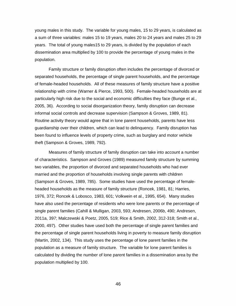
46
young males in this study. The variable for young males, 15 to 29 years, is calculated as
a sum of three variables: males 15 to 19 years, males 20 to 24 years and males 25 to 29
years. The total of young males15 to 29 years, is divided by the population of each
dissemination area multiplied by 100 to provide the percentage of young males in the
population.
Family structure or family disruption often includes the percentage of divorced or
separated households, the percentage of single parent households, and the percentage
of female-headed households. All of these measures of family structure have a positive
relationship with crime (Warner & Pierce, 1993, 500). Female-headed households are at
particularly high risk due to the social and economic difficulties they face (Bunge et al.,
2005, 36). According to social disorganization theory, family disruption can decrease
informal social controls and decrease supervision (Sampson & Groves, 1989, 81).
Routine activity theory would agree that in lone parent households, parents have less
guardianship over their children, which can lead to delinquency. Family disruption has
been found to influence levels of property crime, such as burglary and motor vehicle
theft (Sampson & Groves, 1989, 792).
Measures of family structure of family disruption can take into account a number
of characteristics. Sampson and Groves (1989) measured family structure by summing
two variables, the proportion of divorced and separated households who had ever
married and the proportion of households involving single parents with children
(Sampson & Groves, 1989, 785). Some studies have used the percentage of female-
headed households as the measure of family structure (Roncek, 1981, 81; Harries,
1976, 372; Roncek & Lobosco, 1983, 601; Volkwein et al., 1995, 654). Many studies
have also used the percentage of residents who were lone parents or the percentage of
single parent families (Cahill & Mulligan, 2003, 593; Andresen, 2006b, 490; Andresen,
2011a, 397; Malczewski & Poetz, 2005, 519; Rice & Smith, 2002, 312-318; Smith et al.,
2000, 497). Other studies have used both the percentage of single parent families and
the percentage of single parent households living in poverty to measure family disruption
(Martin, 2002, 134). This study uses the percentage of lone parent families in the
population as a measure of family structure. The variable for lone parent families is
calculated by dividing the number of lone parent families in a dissemination area by the
population multiplied by 100.

47
Single people who have never been married tend to have less responsibilities or
ties to family. According to routine activity theory, they are more likely to participate in
entertainment activities outside of the home and go out in the evening. Therefore, single
people are at greater risk of victimization by strangers as they tend to spend less time at
home and more time in public. People who live alone are at greater risk of personal
robbery as they tend to spend less time at home with family and more time
unaccompanied in locations where crimes may occur (Cohen & Cantor, 1980, 147).
Households consisting of more than one person have greater levels of guardianship than
households with only one person (Cohen & Cantor, 1980, 147). Single people who have
never been married are also more likely to move about and travel as they do not have as
many permanent commitments as a married person such as owning a home, providing
financially for a family, or taking care of others.
Some studies used the percentage of residents that were never married or the
percentage of single person households as a measure of family disruption along with
percentage of single parents (Cahill & Mulligan, 2003, 593; Roncek & Lobosco, 1983,
601). Other studies have used the percentage of the population that was divorced or
separated (Stretesky, Schuck, Hogan, 2004, 827). Cohen and Cantor (1980) used the
number of people living alone to represent single person households (Cohen & Cantor,
1980, 147). Kennedy and Forde (1990) used the number of married and unmarried
people in the population (Kennedy & Forde, 1990, 140). This study uses the percentage
of never legally married people in the population as a measure of marital status. The
percentage of never married in the population is calculated by dividing the number of
single or never legally married people in a dissemination area by the population
multiplied by 100.
Racial heterogeneity is the presence of different racial groups among the
population (Warner & Pierce, 1993, 501). According to social disorganization theory,
racial heterogeneity decreases the cultural transmission of values and decreases social
cohesion. It segments a community, inhibits a neighbourhood’s ability to achieve
consensus, increases mistrust, and impedes communication and interactions (Sampson
& Groves, 1989, 781). Areas high in racial heterogeneity tend to have higher crime rates
(Cahill & Mulligan, 2003, 607). Racial heterogeneity has a greater effect in poorer areas
and areas with lower socio-economic status (Warner & Pierce, 1993, 499). Some
studies have found a positive relationship between racial heterogeneity and burglary but
48
not assault and robbery (Warner and Pierce, 1993, 504). Other studies have found
racial heterogeneity has an effect on both theft and violent crime (Sampson, 1986, 14).
According to Andresen (2006), most American studies measure racial
heterogeneity by the percentage of African American and Hispanic residents in the
population (Andresen, 2006b, 490; Harries, 1976, 372; Roncek, 1981, 80). Many of
these studies only used the percentage of African Americans in the population as a
measure of race (Sampson, 1986, 9; Lockwood, 2007, 198; Martin, 2002, 134; Rice &
Smith, 2002, 312-318; Smith et al., 2000, 499). Due to varied ethnic make-up of
Canada’s population, however, it is more appropriate to use other measures (Andresen,
2006b, 490). Some studies create indices of the relative size and number of different
racial groups in the population (Sampson & Groves, 1989, 784; Cahill & Mulligan, 2003,
593). Other studies use measures of ethnic heterogeneity such as the number of
inhabitants born abroad (Ceccato, Haining, & Signoretta, 2002, 37). The recent
immigrant population has also been used as a measure of ethnic heterogeneity
(Andresen, 2006b, 490; Andresen, 2006c, 259; Andresen, 2011a, 396). Finally, some
studies have used the percentage of visible minorities in the population to measure
racial heterogeneity (Malczewski & Poetz, 2005, 519). This study uses the percentage
of visible minorities in the population as a measure of racial heterogeneity. The
percentage of visible minorities in the population is calculated by dividing the number of
visible minorities in each dissemination area by the population multiplied by 100.
According to social disorganization theory, low socio-economic status is
associated with crime. Low socio-economic status impedes participation in formal and
voluntary organizations, which can decrease formal and informal control and community
supervision of local youth (Sampson & Groves, 1989, 780). Low socio-economic status
can also be a motivation for committing crimes. Socio-economic status can include
measures of income, unemployment, poverty and education. These variables are often
found to be correlated with crime. Studies have found that low socio-economic status
measured by high poverty and low education was a strong indicator of crime (Cahill &
Mulligan, 2003, 607). Alternatively, some studies have found that socio-economic status
had insignificant effects on the rates of theft or personal violence (Sampson, 1986, 12;
Sampson & Groves, 1989, 789). A routine activity theory approach might suggest that
higher socio-economic status and income could increase a person’s ability to purchase
goods and increase the values of targets in an area, thus increasing crime.

49
Socio-economic status and income are measured in a variety of ways. Some
studies have created an index of social disadvantage from a number of variables
including the percentage of residents below poverty level, the percentage of female-
headed households with children, the percentage of unemployed population, and the
percentage of households receiving public assistance (Lockwood, 2007, 198; Stretesky
et al., 2004, 827). Many studies have used the percentage of residents living below the
poverty level as a measure of poverty (Harries, 1976, 372; Cahill & Mulligan, 2003, 593;
Rice & Smith, 2002, 312-318; Sampson, 1986, 8). The number of households with
dependents on social benefits, receiving welfare, or public assistance are also measures
of poverty (Ceccato, Haining, & Signoretta, 2002, 37; Ceccato & Oberwittler, 2008, 194).
Finally, other studies measure high socio-economic status. Sampson and Groves
(1989) used a scale summing the percentage of college-educated population,
percentage of population in professional and managerial positions, and percentage of
population with high incomes (Sampson & Groves, 1989, 784).
Many studies have used the average household income as a measure of socio-
economic status (Malczewski & Poetz, 2005, 519; Harries, 1976, 372; Cahill & Mulligan,
2003, 593; Rice & Smith, 2002, 312-318; Andresen, 2006b, 490; Andresen, 2006c, 260;
Andresen, 2011a, 387; Kennedy & Forde, 1990, 141). Andresen (2006b, 2006c and
2011a) used the standard deviation of average income in addition to average income
(Andresen, 2006b, 490; Andresen, 2006c, 260; Andresen, 2011a, 387). The average
income of the population 15 years or older, not average family income, is the measure
income in this study. For income, the average income of each dissemination area is
already contained in the census data and does not need to be calculated.
Unemployment is also a measure of socio-economic status. Employment is
related to how much income a person can make if they work (Andresen, 2006c, 274).
According to routine activity theory, unemployment has a positive relationship to crime.
Employment takes up a large portion of a person’s time, increasing time spent under
supervision and limiting exposure to potential offenders. Therefore, there is less idle
time to run into potential opportunities for crime (Andresen, 2006c, 274; Bunge et al.,
2005, 20). Employment also provides income for purchasing goods, which can increase
value of targets. Social disorganization theory also assumes a positive relationship
between unemployment and crime. According to social disorganization theory,
employment also provides informal control and increases a person’s ability to integrate

50
successfully into society (Bunge et al., 2005, 20). Youth build positive relationships by
entering the workforce and employment provides them with positive avenues for
achieving status; unemployment can lead to youth exploring other delinquent avenues to
acquiring status (Bunge et al., 2005, 20). Many studies have found a positive
relationship between unemployment and crime (Andresen, 2006c, 269; Andresen,
2006b, 49; Cohen & Cantor, 1980, 153; Kennedy & Forde, 1990, 145-146).
Many studies use the unemployment rate as a measure of socio-economic status
(Andresen, 2006b, 490; Andresen, 2006c, 259; Andresen, 2011a, 396; Malczewski &
Poetz, 2005, 519; Fox & Hellman, 1985, 435-436). Most studies have used the number
of unemployed residents in an area or the percent of residents who were unemployed
(Ceccato, Haining, & Signoretta, 2002, 37; Kennedy & Forde, 1990, 141). Harries
(1976) measured unemployment as the percentage of civilian labour force 16 years and
over who were unemployed (Harries, 1976, 372). This study measures unemployment
by the percentage of unemployed people in the population. Unemployment is calculated
by dividing the number of unemployed people in each dissemination area by the
population multiplied by 100.
Education can be another measure of socio-economic status as it also relates to
a person’s ability to earn income. Educational attainment has a positive effect on crime
as it acts as a protective factor against delinquent behaviour (Bunge et al., 2005, 35).
Low educational attainment is associated with increased risk of crime and delinquency
(Bunge et al., 2005, 35). According to social disorganization theory, areas
characterised by higher education levels will have less crime, as education provides
informal control, attachment to conventional groups and promotes social cohesion.
There are a number of potential measures used to represent education level.
Harries (1976) for example, measured education by the median school years completed
by people 25 years or older (Harries, 1976, 372). Other studies have used the
percentage of residents who were college graduates as a measure of education (Cahill
& Mulligan, 2003, 593; Andresen, 2006b, 490). Other studies have used the percentage
of population with a university degree or or post-secondary education as a measure of
education (Andresen, 2006c, 260; Andresen 2011a, 396-397). Malczewski and Poetz
(2005) used the percent of population over fifteen years with less than a grade nine
education to measure a lack of education (Malczewski & Poetz, 2005, 519). The
percentage of people in the population with a certificate, diploma, or degree as the

51
highest level of education is the measure education in this study. Education is
calculated by dividing number of people with a certificate, diploma, or degree in each
dissemination area by the population multiplied by 100.
The value of dwellings is a common variable used in the analysis of crime
patterns as it represents the level of neighbour affluence. According to routine activity
theory, an increase in average value of dwellings in an area increases the suitability of
targets in the area. Average dwelling value also represents the housing structure of a
neighbourhood. In disagreement with routine activity theory, social disorganization
theory states that areas with higher housing values have more social cohesion and thus
lower crime rates.
Most studies used the median or average value of a dwelling as the measure of
housing value (Cahill & Mulligan, 2003, 593; Rice & Smith, 2002, 312-318; Smith et al.,
2000, 499). Harries (1976) used the median value of owner occupied single-family
housing units as a measure of value of dwellings (Harries, 1976, 372). This study uses
the average value of a dwelling as a measure of neighbourhood affluence. This does
not need to be calculated as the average value of dwelling in each dissemination area is
already contained in the census data.
According to social disorganization theory, household structure can affect crime
rates. The age, type, and density of dwellings, as well as the percentage of renter
occupied versus owner occupied dwellings can be used as measures of housing
structure. Sampson (1986) found that measures of neighbourhood structural density
have strong positive relationships with theft. Neighbourhood instability, including renter
occupied dwellings and residential mobility, strongly influence crime rates by decreasing
social cohesion and social control. Renter occupied dwellings represents a transient
population that can lead to social instability in a neighbourhood. Therefore, a positive
relationship is expected between renter occupied dwellings and crime.
Many studies have used the percentage of rental housing units in an area to
measure housing structure (Cahill & Mulligan, 2003, 593; Andresen, 2006b, 490;
Andresen, 2006c, 260; Andresen, 2011a, 396; Malczewski & Poetz, 2005, 519). Other
studies have used the percentage owner occupied housing (Martin, 2002, 134; Smith et
al., 2000, 499). Some studies have used both the percentage of renter occupied
housing and owner occupied housing (Lockwood, 2007, 198). This study uses the
percentage of renter occupied dwellings of all occupied dwellings in each dissemination

52
area. This is calculated by dividing the number of renter occupied dwellings in each
dissemination area by the number of occupied dwellings multiplied by 100.
Residential mobility is the amount of residents who move and have not lived in
the same house over a certain period. According to social disorganization theory,
residential mobility reflects instability within a neighbourhood and influences crime.
Residential mobility acts as a barrier to forming social ties (Sampson & Groves, 1989,
780). Neighbourhoods with high residential mobility have increased anonymity among
neighbours, weakened primary relationships and decreased informal social control
(Warner & Pierce, 1993, 502). High levels of residential stability are strong predictors of
crime (Cahill & Mulligan, 2003, 607).
There are different ways to measure residential mobility. Ceccato, Haining and
Signoretta (2002) used the number of inhabitants who move into and out of geographical
area as a measure of residential mobility (Ceccato, Haining & Signoretta 2002, 37).
Andresen (2011a) used the percentage of residents who had moved into the census
boundary unit within the past year as a measure of residential mobility (Andresen,
2011a, 396). Other studies used the percentage of movers within the last five years
(Malczewski & Poetz, 2005, 519). Some studies have used the percentage of residents
who had lived in the same house for five or more years to measure a lack of residential
mobility (Harries, 1976, 372; Martin, 2002, 134). Sampson and Groves (1989)
measured a lack of residential mobility by the percentage of residents brought up within
a 15-minute walk from the area in which they currently reside (Sampson & Groves,
1989, 784). Cahill and Mulligan (2003) used the percentage of residents who had lived
in their house since 1970 or for the past 20 years (Cahill & Mulligan, 2003, 593). The
percentage of people in a dissemination area who had moved within the past five years
is the measure residential mobility in this study. This is calculated by dividing the
number of people who had moved within the past five years in each dissemination area
by the population multiplied by 100.
Some of the census variables in the dataset are estimates based on a sample of
20% by Statistics Canada. These variables were the number of occupied dwellings and
the number of renter occupied dwellings, mobility within five years, education, visible
minority, and average income. Some census questions are asked of all Canadians,
while other cultural and economic questions are asked of only a sample of one in five
Canadians. These questions are then weighted to produce estimates for the population

53
(Statistics Canada, 2009a). The weighted results may differ somewhat from the values
found in the actual population due to sampling error (Statistics Canada, 2009a). This
error tends to average out when aggregated to a larger area such as a city, but at the
smaller dissemination area these errors may be more significant (Statistics Canada,
2009a). Also, all counts in census tabulations are subject to random rounding to a base
of five for confidentiality reasons (Statistics Canada, 2013). In this study, the sampling
error due to the 20% sample and random rounding are issues. One dissemination area
has 100.5% visible minorities (210 visible minorities divided by 209 population) and one
dissemination area has 103% renter occupied dwellings (160 renter occupied
dwellings/155 occupied dwellings). This is a limitation of the data and may affect the
results of the study.
There are nine dissemination areas where no population data was available.
This may be due to no people living in those areas, such as provincial and national park
or industrial areas. These dissemination areas, accounting for less than 1% of the
sample, are removed from the analysis. Figure 3 shows the location of the
dissemination areas removed from the analysis due to having zero population. The
dissemination areas shown in yellow are included in the analysis while the dissemination
areas shown in white are the ones removed from the analysis. These removed areas
are not clustered in one location and do not contain a university.

54
Figure 3. Map of dissemination areas in Ottawa included in the analysis
Seven dissemination areas contain population data but are missing other census
variables. This is due to the small population size of these dissemination areas. For
reasons of confidentiality, there must be a minimum population of 250 residents in a
census unit to have socio-demographic and socio-economic variables released
(Andresen, 2006b, 492). This should not bias the results, as it is only a small
percentage (less than 1%) of the sample. Unfortunately, one of these dissemination
areas with incomplete census data is the dissemination area that contains Carleton
University. The census variables for this dissemination area need to be estimated to
correct for this problem. This is done by taking an average of the values from the
surrounding dissemination areas. There were 17 dissemination areas surrounding and
touching the border of the dissemination area that contains Carleton University. The
average values of the 17 surrounding dissemination areas are calculated for each of the
eleven independent variables. There is census data for certain variables in this
dissemination area: population, young males and never married. The estimated average
values for these variables are compared to the actual census values to provide an
indication of the validity to the approximation. The estimated and actual values for this
dissemination area are very similar. Table 3 shows the comparison between the
estimated values and the actual values of the census data for the dissemination area

55
containing Carleton University. This estimation procedure for this dissemination area
represents a successful approximation of the actual values for the missing census
variables.
Table 3. Comparison between estimated values and the actual values of the census data for dissemination area containing Carleton University
Actual Census Value Estimated Census Value % Difference
Population 704 723.82 2.82%
Young males 12.07 11.66 -3.40%
Never married 34.80 36.92 6.09%
4.2.4 Dependent Variables: Burglary, Robbery, and Motor Vehicle Theft
This study uses publicly available weekly activity reports for 2006 from the
Ottawa Police Service’s website (http://www.ottawapolice.ca) as a source of crime data.
These activity reports are weekly listings criminal activity reported to or identified by the
police and contain information on the date, time, district, block face address, and type of
offence. As with other police reported measures of crime, such as Uniform Crime
Reporting (UCR), the use of weekly activity reports have some disadvantages. These
police reported measures of crime represent the number of crimes that have come to the
attention of the police and may reflect biases in official reactions to crime (Warner &
Pierce, 1993, 494). High levels of crime in an area may actually represent higher levels
of policing rather than higher levels of occurrence (Warner & Pierce, 1993, 494). Police
may be more likely discover a crime, attend a call, or make an arrest in areas where
there are known crime problems (Warner & Pierce, 1993, 494). Police discretion of can
lead to non-reporting of crimes and underrepresentation in official crime statistics
(Herbert, 1982, 4). Proactive policing of crimes such as prostitution, drug possession,
pornography, drinking and driving, may reflect policing patterns and priorities more than
actual crime occurrence (Bottoms & Wiles, 2002, 625).
Other possible sources of police reported crime data are calls for police service
and victimization data. These sources are not affected by police decision making;
however, they do rely on the public’s willingness to reporting of crime and recollection of
events. Calls for service are requests for police service made by the public to a police
department, either directly to the department or indirectly through an emergency
dispatch service (Andresen, 2006b, 492). Calls for service data records police activity,

56
like the weekly activity reports; however, these include all the calls received by the police
department regardless of whether police respond to the call or not. Calls for service,
however, do not measure actual occurrence of crime, as the police have not
substantiated the calls (Andresen, 2006b, 492). Calls for service data can over-
represent some crimes, such as noise complaints, if more than one person reports the
crime to police (Browser & Carroll, 2007, 272). They can also under-represented other
crimes, such as assaults, if police are present in the downtown bar area and detected
crimes themselves without receiving calls for service (Browser & Carroll, 2007, 272).
Official crime measures require that the public report crimes to the police. It is
understood that a large portion of crimes occur but go unreported to the police. This is
known as the ‘dark figure of crime’. This can be due to the victim feeling ashamed or
threatened, feeling the crime was not important enough to report to the police, not
wanting to have involvement with the police, or the crime going unnoticed (Herbert,
1982, 4; Brantingham & Brantingham, 1984, 49). Some types of offences are less likely
to be reported to the police, such as domestic violence, drug crimes, and white-collar
crimes; while other crimes such as motor vehicle theft, arson and murder have higher
reporting rates (Herbert, 1982, 5; Bruce et al., 2004, 200). Under reporting of crime
varies by socio-demographic groups, context of the crime, and environmental settings
(Nelson et al., 2001, 252). Police reported crime rates might reflect changes in the
occurrence of crime or simply changes in the public’s reporting of crime (Brantingham &
Brantingham, 1984, 50).
Victimization surveys use uniform definitions of crime across jurisdictions
providing comparable data (Cohen & Land, 1984, 501). They are a more accurate
measure of the actual amount of crime in an area as they identify crimes not reported to
police, including minor crimes not considered serious to report (Cohen & Land, 1984,
501). Victimization surveys have higher offence rates than police reported data (Cohen
& Land, 1984, 501). Victimization surveys also have their limitations. They only capture
information from residents of an area, and not visitors, commuters, or homeless people
who may have been the victim of crime (Cohen & Land, 1984, 501). They also rely on
the respondents’ memory and ability to recall the incident and the respondent’s
willingness to discuss the offence such as a rape or assault (Cohen & Land, 1984, 501).
In addition, victimization studies require a large sample size in order to be spatially
representative of small areas within a city (Brantingham & Brantingham, 1981, 23).

57
Cohen and Land (1984) conducted a study comparing police reported Uniform
Crime Reports data to National Crime Surveys on victimization (Cohen & Land, 1984,
500). The authors examined police data and victimization data in 26 American cities for
six types of crime: rape, aggravated assault, robbery, burglary, theft, and motor vehicle
theft (Cohen & Land, 1984, 508). All the cities chosen were large central cities (Cohen &
Land, 1984, 511). They also included census data on socio-demographic characteristics
of the population such as city size, density, mobility, racial and ethnic heterogeneity,
poverty, unemployment, age, household size, divorced population, and size of police
force (Cohen & Land, 1984, 508-510). The authors used ordinary least squares
regression for each of the crime types with the socio-demographic variables (Cohen &
Land, 1984, 514). The authors found that the socio-demographic variables had a
differential impact on the rates of reporting crime to police versus reporting crimes in
victimization surveys (Cohen & Land, 1984, 521). When the authors controlled for the
socio-demographic variables they found a much closer correspondence of police and
victimization rates for four of the six crime types, motor vehicle theft, robbery, burglary,
and rape, but not aggravated assault and theft (Cohen & Land, 1984, 520). This finding
suggests that the police reported data for motor vehicle theft, robbery and burglary
would be an acceptable measure of crime.
Another study by Booth, Johnson and Choldin (1977) examined the effect of
eight socio-demographic factors on the incidence of crime data collected through
victimization surveys and police reported official crime data (Booth, Johnson, & Choldin,
1977, 187). The authors examined the two types of crime data in 26 American cities in
the mid 1970s for robbery, burglary and motor vehicle theft (Booth et al., 1977, 190).
The authors used multiple regressions to assess the effect of the each independent
variable on the two types of crime measures (Booth et al., 1977, 190). In seven of the
eight independent variables, the relationship changed directions indicating that the two
measures were not measuring the same phenomenon (Booth et al., 1977, 194). The
authors found that the two types of crime measures gave different results and they
reached different conclusions for each type of offence depending on the type of crime
measure used (Booth et al., 1977, 196). The two crime measures were more reliable
indicators for motor vehicle theft than robbery and burglary (Booth et al., 1977, 195-196).
However, there was no evidence of one measure being a more valid indicator of crime
than the other (Booth et al., 1977, 196).

58
Police activity reports are a useful measure of crime as they contain timely,
reliable and accurate data on offences and their geographical location. Police data often
records offences at the street or address level, rather than a general area, which is ideal
for identifying crime patterns and trends using GIS (Nelson et al., 2001, 257). For
crimes such as burglary, robbery, and motor vehicle theft a large proportion of these
crimes are reported to the police, as the victims need to report the crime for insurance
purposes. For crimes where the victim was present during the offence, such as robbery
and assault, the exact date and time of the offence is often known (Bruce et al., 2004,
200). Whereas in crimes where the victim was not present at the time of the offence,
such as motor vehicle theft and burglary, the exact date and time of the offence may not
be known (Bruce et al., 2004, 200). On a larger scale, such as a comparison between
police forces, official police statistics can be misleading. Different police departments
have different definitions, recording and enforcement practices that can influence the
accuracy of information obtained by police (Cohen & Land, 1984, 400). On a smaller
scale within a city, where police department recording practices are the same, they
provide a better indication of differences between neighbourhood crime levels (Bottoms,
2007, 534-535). According to Nelson, Bromley, and Thomas, “police data, whatever the
deficiencies, are undoubtedly the most comprehensive and reliable data source
available” for exploring crime patterns and characteristics (Nelson et al., 2001, 252).
The three dependent variables are burglary (residential and commercial), robbery
(individual, commercial, and other) and motor vehicle theft. Burglary is a theft that
occurs without the presence of a victim. There are commercial and residential burglaries
that have different patterns. Commercial burglaries tend to occur in central business
districts, commercial, and industrial areas while residential burglaries tend to occur in
residential areas (Harries, 1980, 94). Residential burglaries occur mainly in the daytime
while residents are away at work or school while commercial burglaries occur mainly in
the evening or weekends when businesses are closed (Dunn, 1980a, 13). Burglary
patterns are influenced by the environment (Evans, 1989, 88). Proximity to open spaces
and major roadways increases the risk of burglary (Evans, 1989, 101). Physical barriers
such as rivers and roadways can decrease chance of an offender crossing the barrier
between areas to commit a burglary while, connectors such as transit, and increased
chance of an offender committing an offence across areas (Clare, Fernandez, & Morgan,
2009, 152).

59
Social capital and collective efficacy in neighbourhoods decreases the likelihood
of residential burglary as the presence of community is a key factor in maintaining order
despite the criminogenic conditions (Martin, 2002, 132). Burglary is related to income,
geographic location and vulnerability (Harries, 1980, 95). Studies have found that
residential burglaries tend to occur in outer city neighbourhoods characterised by high
socio-economic status and single-family houses (Ceccato, Haining, & Signoretta, 2002,
34). Neighbourhoods characterised by higher socio-economic status tend to have lower
risk of residential burglary (Malczewski & Poetz, 2005, 523). There is a positive
relationship between residential burglaries and the average value of dwellings
(Malczewski & Poetz, 2005, 523). Socially mixed neighbourhoods with high population
turnover tend to have more crime; therefore, relatively deprived neighbourhoods with
high immigrant population and low income have higher burglary rates (Malczewski &
Poetz, 2005, 523). Age composition has a strong effect on residential burglary due to
the proportion of youth committing burglary in their neighbourhood (Martin, 2002, 141).
Poverty and residential stability are also positively related to residential burglary (Martin,
2002, 141).
Burglary offenders tend to come from socially disadvantaged areas and commit
crimes close to home in their neighbourhood or the surrounding areas within their routine
activities (Ceccato, Haining, & Signoretta, 2002, 34; Malczewski & Poetz, 2005, 523).
The risk of residential burglary tends to increase in areas with high socio-economic
status if they are located near areas with high offender rates (Bottoms & Wiles, 2002,
628). The highest risk of burglary tends to be in areas adjacent to the city centre, while
the lowest risk tends to be in the peripheral areas of the city (Malczewski & Poetz, 2005,
516-518). Therefore, crime decreased as you moved away from the city centre
(Malczewski & Poetz, 2005, 518). Areas of lower socio-economic status are at risk if
they are close to the city centre (Ceccato, Haining, & Signoretta, 2002, 34). The relative
attractiveness of an area is a factor. Areas with higher value dwellings are more at risk
as they make more attractive targets than lower value dwellings (Ceccato, Haining, &
Signoretta, 2002, 34). The number of dwellings units in an area also increases the risk
of burglary, as there are a greater number of available targets (Rengert, 1981, 198).
Housing type has also been found to influence the risk of residential burglaries; with
detached housing having the lowest risk and semi-detached housing and flats having the
highest risk (Bowers, Johnson, & Pease, 2005, 10). The risk of burglary victimization

60
also increases with a lack of guardianship when activities take people away from the
home (Kennedy & Forde, 1990, 142).
Robbery is a type of theft that involves a direct confrontation with the victim and
taking something by force or threat of force; therefore, robbery is a personal and violent
crime (Cook, 1983, 3). Robbery has a profit motive and usually involves some
premeditation (Lenz, 1986, 97). Commercial targets for robbery can include banks,
pharmacies, jewellery stores, bars, and restaurants; however, gas stations and
convenience stores tend to have the greatest number of robberies (Harries, 1980, 98).
Personal targets of robbery are usually victims on the street. Street robbery is usually
occurs in an outdoor public place (Bernasco & Block, 2011, 38). Commercial robbery
locations tend to be more spread out than personal robbery locations, as personal
targets are more likely to be clustered (Lenz, 1986, 103). Most robbers live areas high in
poverty and commit crimes close to home in the areas adjacent to the one they live in
(Dunn, 1980a, 12; Cook, 1983, 12). Robbers tend to select targets based on minimum
effort and maximum benefit, so they do not travel great distances unless there is an
incentive to do so (Van Koppen & Jansen, 1998, 244). More experienced robbers will
travel greater distances and chose more difficult targets than less experienced robbers
(Van Koppen & Jansen, 1998, 230).
Opportunity, temporal considerations, and neighbourhood social indicators are
important factors influencing robbery patterns (Harries, 1980, 99). The convergence of
potential victims and offenders in public spaces during the course of leisure activities is
important in determining the occurrence of robbery (Ceccato & Oberwittler, 2008, 189).
Robberies tend to take place at night rather than in the daytime (Ceccato & Oberwittler,
2008, 186). Robberies tend to take place in densely populated urban areas as they
provide anonymity to offenders and a high concentration of potential targets (Cook,
1983, 11). Land use is a strong predictor of street robbery (Smith et al., 2000, 511).
Robberies tend to occur in the city centre, in public spaces such as the street, or semi-
private leisure and commercial areas (Nelson, Bromley, & Thomas, 2001, 251). City
centres with stores, commercial establishments, and financial institutions relatively
attractive when adjacent to areas of low income and physical deterioration (Dunn,
1980a, 12). Robberies can take place in areas within two blocks from a major
transportation artery, on streets with little traffic, and along thoroughfares (Cook, 1983,
12; Harries, 1980, 98). Lockwood (2007) found that robbery also has a strong

61
correlation with recreational land use as many robberies take place in parks (Lockwood,
2007, 204). Blocks with a crime generator or crime attractor have high number of
robberies and all types of crime generators and attractors increase the number of
robberies in a block as well as in adjacent blocks (Bernasco & Block, 2011, 48-49).
Robbery occurs in areas with public, semi-public, and mixed land uses and social
disadvantage (Lockwood, 2007, 203). Smith et al. (2000) found that socio-demographic
variables were stronger predictors of street robbery than routine activity variables (Smith,
Frazee, & Davidson, 2000, 511). Race, single parent households, low value dwellings,
distance from city centre, and owner occupied dwellings are all predictors of street
robbery (Smith et al., 2000, 511). Robberies also tend to take place in areas
characterised by a high percentage of unemployment, lower education, lower median
income, and few married people (Dunn, 1980a, 12). Poverty, race, and ethnicity are all
positively related to the number of robberies (Bernasco & Block, 2011, 50). Cohen and
Cantor (1980) found that families with lower incomes, people who were 50 or older, and
homemakers have lower risk of personal robbery victimization while families with higher
incomes, people ages 16 to 29 years, and people who live alone or are unemployed are
at higher risk (Cohen & Cantor, 1980, 153). Age is one of the strongest predictors of
robbery victimization (Cohen & Cantor, 1980, 155).
Motor vehicle theft can occur for three primary motives, recreational joyriding,
transportation, and profit (Fleming, Brantingham & Brantingham, 1994, 49). Joyrides
tend to be committed by younger offenders who want to steal a car for temporarily for
status of thrill seeking (Fleming et al., 1994, 49). Transportation driven motor vehicle
thefts can include stealing a car for temporary or long-term use of the vehicle for a ride
home or use of the vehicle in other criminal activity (Fleming et al., 1994, 49). Profit
motivated motor vehicle thefts tend to be more organized and planned and can include
stealing a vehicle for a chop shop, or stripping of the vehicle for parts, or re-selling the
vehicle (Fleming et al., 1994, 49). Geographically, motor vehicle theft rates have little
relationship to other crime rates (Rice & Smith, 2002, 304). Vehicles are different from
other property crime targets because they are mobile (Rice & Smith, 2002, 306).
Routine activities can influence motor vehicle theft. Motor vehicle theft tends to
occur where there is heavy traffic and activity and many cars to steal (Rice & Smith,
2002, 306). Motor vehicle theft is highly concentrated around major roadways and
shopping centre parking lots, while a smaller portion of motor vehicle theft occurs in

62
residential areas (Wuschke, 2008). Parking lots used by commuters such as at transit
stations and central business districts may be easier targets as the vehicles are left for
longer periods of time with less surveillance and guardianship (Bottoms & Wiles, 2002,
628). Motor vehicle thefts in residential areas tend to occur at night, while motor vehicle
thefts from city centres tend to occur in the daytime (Bottoms, 2007, 538). Most motor
vehicle thefts occur when cars are parked on the street near the owners’ home
(Ceccato, Haining, & Signoretta, 2002, 33). Cars are four times more likely to be stolen
from the street than from a garage (Clarke & Mayhew, 1994, 94). The risk of motor
vehicle theft is higher for drivers living in apartment buildings and rental
accommodations than homes, as the parking tends to be less secure (Clarke & Mayhew,
1994, 94). The number of activity nodes and the characteristics of a location, including a
lack of visible signs of security and poor environmental design, can increase the
likelihood of repeat victimization of motor vehicle theft (Levy &Tartaro, 2010, 86-87).
However, activity nodes were better predictors of motor vehicle theft in commercial
locations than residential locations (Levy &Tartaro, 2010, 90).
The structures and social characteristics of the immediate and surrounding area
influence motor vehicle theft (Rice & Smith, 2002, 328). Motor vehicle theft is often
contingent on the extent of social disorganization in the area (Rice & Smith, 2002, 328).
Some studies have found that motor vehicle theft occurs in areas with social problems,
areas with multi-storey housing, and low socio-economic status (Ceccato, Haining, &
Signoretta, 2002, 33-34). While other studies have found that motor vehicle theft occurs
more frequently in city centres (Bottoms & Wiles, 2002, 626). These poorer and inner
city areas may be more at risk because there may be more drivers parking on the street
(Clarke & Mayhew, 1994, 94). Low building values and single parent households
increase motor vehicle theft, especially if low building values and single parent
households are located on the same block as stores, shops, or commercial places (Rice
& Smith, 2002, 323-324). A disproportionate amount of the motor vehicle offences are
committed by young people for the purpose of joyriding rather than older, organized, and
profit motivated offenders (Fleming et al., 1994, 47).
The number of incidents and the location and time for each type of offence is
obtained from the Ottawa Police Service weekly activity reports. The weekly activity
reports have a total of 7,813 cases. There are 4,147 cases of burglary; 1,506 of which
are commercial and 2,641 are residential. Burglary accounted for over half of the cases

63
(53%). There are 783 cases of robbery; 146 of which are commercial, 256 are
individual, and 378 are other robberies. Robbery accounted for 10% of the cases.
There are 2,883 cases of motor vehicle theft in the dataset, accounting for 37% of cases.
Table 4 shows the number and percent of cases for each crime type in the Ottawa
Police Service weekly crime reports.
Table 4. Ottawa Police Service weekly crime report data
Crime Type Number of Cases Percent of Cases
Burglary 4,147 53.1%
Commercial 1,506 19.3%
Residential 2,641 33.8%
Robbery 783 10.0%
Commercial 146 1.9%
Individual 256 3.3%
Other 378 4.8%
Motor Vehicle Theft 2,883 36.9%
Total 7,813 100.0%
The weekly activity reports for 2006 from the Ottawa Police Service came in text
file format. These need to be converted into an excel spreadsheet. A custom script
written using PHP programming language converts the text files to excel format. Data
filtration or removing unnecessary data such as police narratives is done during this
process (Bruce et al., 2004, 28). The resulting excel spreadsheet contains the following
information: case number, week, month, day, year, date, time, AM/PM, district, crime
type (breaking and enter, robbery, motor vehicle theft), type of target (commercial,
residential, personal, other), 100 block, and street.
Errors can occur in the data transfer process from text format to excel by
manipulating the data (Boba, 2005, 97). Some possible errors that can occur are
duplication of records, missing information or incomplete address and offence type, and
incorrect date/time (Malczewski & Poetz, 2005, 517). The excel data are manually
checked and compared to the text data for errors in the script. Errors found in the type
of crime categories are the result of inconsistent headings in the text files that did not
transfer properly to excel format. These errors need to be corrected manually.

64
The weekly activity reports contain block face addresses. A block face address,
or street segment, is one side of the street between two consecutive features
intersecting that street, such as other streets or boundaries of geographical areas
(Statistics Canada, 2007, 13). Block faces are used to generate block face
representative points from street and address information (Statistics Canada, 2007, 13).
These block face addresses are truncated from a specific address to the 100-block level
in order to preserve the geographical information while keeping the individual’s address
private. For example, 123 University Drive would appear as 100 block of University
Drive. Any address between 100 and 199 on a street is grouped into the 100 block.
Roncek suggested using the block level for statistical analysis as the block is the basic
ecological unit of the city (Harries, 1980, 84).
There are potential accuracy issues in associated with using address level crime
data. There are some cases when police cannot associate an offence with a specific
building or address. This is when a crime occurs in a public space, such as street
corner, sidewalk, bus stop, and roadway. Instead, these offences are often assigned to
a nearby intersection (Buerger, Cohn, & Petrosino, 1995, 245). This could potentially
cause some problems in hot spot analysis as a large number of offences are scored to
intersections, despite the fact that most crimes do not actually occur in intersections
(Buerger et al., 1995, 245). However, the data in this study is aggregated to the
dissemination area level so the intersection issue will not affect the results.
In order to map the geographical location of the weekly activity report data, a
random number generator is used to assign a specific address to the 100-block face. A
number between 0 and 99 is randomly assigned to each address. For example, if the
block face address is 800, the random number generator provides 895 as the street
number. This allows crime locations to be evenly distributed on either side of a street.
The potential issue of interpolation, or geocoding a point to an incorrect position on a
street segment, is not a problem in this study, as the data will be aggregated to the
dissemination area (Andresen, 2011a, 396). The street number is combined with the
street name and type in a single field for geocoding.
The address data in this study are checked for missing or inconsistent data that
might lead to problems in the geocoding. The address data are manually cleaned to fix
problems such as typos, abbreviations, spelling mistakes, punctuation, aliases,
malapropisms, generalizations, wrong directional identifiers, wrong street suffix or street

65
type, record and field truncations, invalid entries and extraneous errors to ensure the
addresses are written in the same format and can be geocoded successfully (Bruce et
al., 2004, 144-147). In preparing the data for geocoding, the data are checked to ensure
there are spaces between the street number and street names. For intersection
addresses, the data are checked to replace “and” with an ampersand to separate two
street names.
The crime data in the form of street addresses are geocoded in ArcView 3.3 GIS,
in order to generate maps and join the dependent variables with the independent
variables spatially. Geocoding is a method of transforming an address into precise
geographic x and y coordinates and join crime data with geographic data for spatial
analysis (Anselin, Griffiths, & Tita, 2008, 101; Boba, 2005, 11). Geocoding is an
automated way to map high volume, address level crime data from a database into a
point on a map (Ratcliffe, 2004, 61). Geocoding software assigns coordinates to
addresses by locating the record in the index street table with a matching street name,
type, prefix, suffix, and street number (McCarthy & Ratcliffe, 2005, 50). The side of the
street, on which the incident is located, is determined by odd and even street numbers
(McCarthy & Ratcliffe, 2005, 50). A multi-step geocoding process is best to ensure the
highest level of accuracy (Groff, Weisburd, & Morris, 2009, 70).
The road network for Ottawa obtained from Statistics Canada
(http://www12.statcan.gc.ca/census-recensement/2011/geo/RNF-FRR/index-2011-
eng.cfm) is used as the reference theme for geocoding. The reference theme was
already prepared for geocoding. The address table is the dataset of crime incidents
made from the police activity reports with the addresses for each crime location to be
geocoded as points on the map of Ottawa. The addresses in the crime table are
standardized to ensure all numbered streets have a street type associated with them
(Andresen, 2006a, 10). This is done using an address standardiser in ArcView 3.3.
ArcView 3.3 is used to batch match the crime locations by comparing the addresses in
the crime table to the street addresses in the reference theme to look for matches. Each
matched point address is added as a point in a new geocoded theme. Missed
addresses can sometimes be corrected manually but the number of cases often
precludes correcting every single address, especially if information is missing (McCarthy
& Ratcliffe, 2005, 52; Lersch, 2007, 235). There can also be cases where the addresses
are incomplete, missing, or the offences take place in a location that is not recognized by

66
the address database (Craglia, Haining, & Wiles, 2000, 714). These cases may need to
be removed if they cannot be corrected.
During the geocoding process, 2,500 cases do not match initially. Once the data
are geocoded, adjustments are made to increase the hit rate and correct any partial
matches or misses (Boba, 2005, 89). There were some addresses that contain 0 as the
street number due to the random number generator. These are given a random number
between 1 and 99. There are some addresses that do not contain a street type. These
addresses are searched in google maps to determine a street type. By Ward Market is
an example of a street name that does not match. After using the closest match to fixe
these errors, 584 cases cannot be geocoded. This results in a successful hit rate of
92.5% that is higher than Ratcliffe’s minimum acceptable hit rate of 85%.
Achieving a 100% successful geocoding process is rare. The geocoding process
of transforming address data to x, y coordinates provides the potential for error
(Andresen, 2009, 338). Sometimes the geocoding algorithm has difficulties locating
specific addresses due to problems with insufficient information, incorrect, or non-
standardized information in police records (Ratcliffe, 2004, 65). It is rare for any address
verification to take place in the process of compiling police records (Ratcliffe, 2004, 65).
Therefore, there can be errors in the data including the omission of address information,
spelling errors, new addresses not recognized by the program, incorrect prefixes and
suffixes, use of abbreviations, incorrect street types, use of landmarks, out of range
addresses, and addresses that do not exist (Ratcliffe, 2004, 65; Boba, 2005, 326). Any
error in geocoding results in the address not being matched to a record in the indexed
street table and a crime not being identified (McCarthy & Ratcliffe, 2005, 52). This can
lead to biased in spatial patterns (Andresen, 2009, 338). The accuracy of the analysis
depends on the accuracy of the spatial data, the accuracy of the geocoding, and
achieving a high level of geocoding success (McCarthy & Ratcliffe, 2005, 46; Ratcliffe,
2004, 61).
Jerry Ratcliffe (2004) developed a minimum reliable geocoding hit rate for crime
data. A hit rate is the percentage of unit records in a crime database that are
successfully geocoded (Ratcliffe, 2004, 61). The minimum reliable hit rate is based on a
number of different crime patterns and a Monte Carlo simulation (Ratcliffe, 2004, 61-62).
The Monte Carlo simulation used random samples resembling real world spatial
problems and generated sets of values to run the simulation multiple times with each run

67
randomly removing a percentage of the points until it fails to resemble the 100% map in
magnitude of points or distribution of values (Ratcliffe, 2004, 67). His minimum reliable
hit rate is 85%; any less than 85% and the results may be unreliable (Ratcliffe, 2004,
61). For example, a 90% hit rate means that one in ten addresses in the crime data are
not geocoded (Ratcliffe, 2004, 70). Ratcliffe’s minimum reliable hit rate has become the
standard upon which most authors in the crime-mapping field assess the success of a
geocoding procedure (Andresen, 2009, 338; Groff, 2011, 179).
One consideration to this minimum acceptable hit rate is that geocoding errors
are usually not randomly distributed in time and space (Ratcliffe, 2004, 70). For
example, a new street may contain multiple crime incidents that are not able to be
geocoded (Ratcliffe, 2004, 70). Before geocoding, it is best to examine the data and
determine if there are any patterns of errors in the addresses and use an address
scrubbing routine to correct common errors such as spelling mistakes, remove unwanted
text, and prepare the addresses for increased geocoding efficiency (Ratcliffe, 2004, 70).
It is also important to determine if there are any patterns within the missed addresses
that would affect the results of the analysis (Ratcliffe, 2004, 70). Some of the geocoded
addresses fall outside of the Ottawa city limits and do not have corresponding
dissemination areas. These addresses are removed from the analysis. Originally, the
data contained 1,275 dissemination areas with 7,813 crimes. This reduced the total
number of cases to 1,266 dissemination areas with a total number of 7,229 crimes.
Table 5 shows the number and percentage of the crimes geocoded.
Table 5. Geocoded dependent variables
Number of Crimes Percent of Crimes
Burglary 3,850 53.3%
Robbery 712 9.9%
Motor Vehicle Theft 2,667 36.9%
Total Crimes 7,229 100.0%
There are 1,032 dissemination areas (81%) that contain crimes and 243
dissemination areas (19%) that do not contain any crimes. The maximum number of
crimes in each dissemination areas is 90 with a mean of 5.7. There are 902
dissemination areas containing burglaries. The maximum number of burglaries in a
dissemination area is 42 with a mean of 3.0. There are 319 dissemination areas

68
containing robberies. The maximum number of robberies in a dissemination area is 20
with a mean of 0.6. There are 715 dissemination areas containing motor vehicle thefts,
with a maximum of 62 motor vehicle thefts in a dissemination area and a mean of 2.1.
Using both the crime data and census data as data sources, relies on secondary
analysis. This can lead to some limitations. First, secondary data only approximates the
type of data needed to test a hypothesis as the data is originally collected for different
purposes (Frankfort-Nachmias & Nachmias, 2000, 279). As police, not researchers,
collect crime data, this is a common issue in criminological research. In addition, the
large scale and high costs associated with collecting census data often precludes this
type of data collection for researchers. Second, the researcher may have insufficient
information about how the data is collected including possible sources of biases and
errors (Frankfort-Nachmias & Nachmias, 2000, 279). The weekly crime reports rely on
the Ottawa Police Service accurately recording the time and location of incidents, as well
as recording every incident they attend.
4.2.5 Spatial Joining of the Variables
To aggregate the crime data to the dissemination area, an areal interpolation
process in ArcView 3.3 is used to sum all the cases of each variable that fall within a
dissemination area and provide a collection of attributes for each dissemination area
(Murray et al., 2001, 314). Spatially joining the crime data points with the dissemination
area polygons, allows spatial analysis to be performed between the crime data and the
socio-demographic and socio-economic data. The Geo Processing Wizard in ArcView
3.3 is used to spatially join the crime data points to the census data polygons. First,
each point is assigned to a polygon using the assign data by location option and an
inside join. This uses the spatial relationship to join the attribute table of the crime data
to the attribute table of the dissemination area that share the same location. This
assigns a polygon number to a crime data point if it falls inside the polygon. Then the
dissolve feature is used to aggregate the crime data points and provide a count of all
points in each polygon based on the dissemination area attributes. This associates the
count of points in each polygon with the polygon file. This is done to allow the
calculation of rates for each polygon.
This joining and dissolving process is repeated four times for each of the crime
categories. First, the motor vehicle points are joined and dissolved to the dissemination

69
area polygons. Second, the burglary points are joined and dissolved to the
dissemination area polygons. Third, the robbery points are joined and dissolved to the
dissemination area polygons. Fourth, the total for all crimes points are joined and
dissolved to the dissemination area polygons. This joins the two tables into one table
that contains the census variables and the associated burglary, robbery, motor vehicle
theft and total of all crimes counts for each dissemination area in Ottawa.
4.2.6 Calculating Crime Rates
This study uses crime rates to examine how one area differs from others. Crime
counts are the number of crimes per dissemination area. Crime counts do not take into
consideration variations in distribution of people within a city, making comparisons
between dissemination areas difficult. Crime rates are the number of crimes per 1,000
population in a dissemination area. Crime rates are used to normalize the variables and
display the number of crime divided by a common denominator (Bruce et al., 2004, 207).
For crime rates, there is often debate about the best type of denominator used to
reflect crime in an area. The most common denominator used is the residential
population from the census. However, there are limitations associated with using
residential population based crime rates in geographical crime analysis (Andresen,
2007, 2427). These can be problematic because not all targets are distributed evenly
amongst the population and the entire population may not be at risk (Harries, 1980, 11).
This is especially problematic in areas such as central business and entertainment
districts where a large number of people visit the area at different times of day, but do
not live in the area. This may lead to artificially high offence rates in city centres based
on resident population (Bottoms & Wiles, 2002, 626).
An alternative crime rate calculation would be to use the ambient population,
which better reflects the number of people who travel to the city centre during the day
and therefore the number of potential targets and offenders for some types of crime.
The ambient population is the 24-hour average estimate of the expected population
present in a squared kilometre area at any time of day or day of year using daily and
seasonal population movements (Andresen, 2011b, 195; Andresen & Brantingham,
2008, 269). This is done by transforming the census-based population using a
probability coefficient and calculating the relative attractiveness of areas using road
proximity, slope, land cover, and nighttime lights (Andresen, 2011b, 195-196; Andresen

70
& Brantingham, 2008, 269). In cases where the targets are mobile, measuring crime by
ambient population may be more useful. Residential population works for burglary crime
rates, however, ambient population works best for violent crimes rates such as robbery,
assault, sexual assault and homicide (Andresen, 2011b, 194). There are differences
between the ambient and census populations in cities (Andresen, 2011b, 196). In a
study of crime in Vancouver using ambient population as the population at risk,
Andresen (2011b) found the correlations between the resident and ambient based
violent crime rates were not dissimilar at the census tract level but were very different at
the dissemination area level (Andresen, 2011b, 200-201).
For specific types of crimes, there are different denominators that provide better
measures of crime occurrence. Opportunity based crime rates using crime specific
denominators to reflect the targets at risk relate the occurrence of crime to
environmental opportunity rather than to a population base (Harries, 1981, 148-149).
The number of households or dwellings measures residential burglary rates more
accurately and the number of registered vehicles or parking spaces may be a better
measure of motor vehicle theft rates (Bottoms & Wiles, 2002, 625; Harries, 1981, 149).
For commercial robbery and burglary, the number of commercial units may be
appropriate (Harries, 1981, 150). For street robbery, the ambient population may
represent the number of possible victim present in the area throughout the day (Harries,
1981, 151). Opportunity based crime rates are more useful for subclasses of crime
types, such as commercial robbery or residential burglary rather than all robberies or all
burglaries, as they can be matched with specific denominators representing the
opportunity for crime (Harries, 1981, 165). However, for the purposes of this study,
residential population as per the 2006 census is used as the denominator for crime
rates, as follows:
Crime rate =C/Px1000
where C= crime count, P= population. Crime rates are calculated for each dissemination
area by calculating a new field from the crime count field and the population field using
the above equation. This new field calculation is repeated for each of the four crime
categories: burglary, robbery, motor vehicle theft, and total of all crimes. Due to the lack
of population data in nine of the dissemination areas, the crime rates can only be
calculated for 1,266 cases. However, these nine dissemination areas are removed from
the analysis.

71
4.3. Data Analysis
A number of studies have conducted spatial regression analysis to examine the
spatial patterns of crime within a city. Kamber, Mollenkopf and Ross (2000) examined
the spatial patterns of burglary, robbery, and motor vehicle theft in Brooklyn. The
authors used geocoded address level crime data from the New York Police
Department’s online complaint system (Kamber, Mollenkopf & Ross, 2000, 107). They
also used 1990 census data including the socio-demographic characteristics of age,
gender, race, ethnicity, income and family structure (Kamber et al., 2000, 108). The
crime data were aggregated to the census tract level to match the census data (Kamber
et al., 2000, 109). The authors used local indicators of spatial autocorrelation (LISA) to
identify crime hot spots (Kamber et al., 2000, 113). The authors tested for
autocorrelation using global Moran’s I in SpaceStat software (Kamber et al., 2000, 114).
From the LISA analysis, the authors found motor vehicle theft values were dispersed
while robbery values were spatially concentrated (Kamber et al., 2000, 114).
They also conducted spatial regression analysis on the rate of residential
burglary using weighted spatial lag variables (Kamber et al., 2000, 116). They reduced
the model to include only the variables that suffered the least from high inter-correlations
(Kamber et al., 2000, 116). The authors found that the variables in the final burglary
model explained a large amount of the variance (Kamber et al., 2000, 117). The number
of single parents in a census tract had a moderate significant relationship with burglary,
while race and the number of single adults had small but insignificant relationships with
burglary (Kamber et al., 2000, 117).
Kennedy and Forde (1990) used routine activity theory to examine crime
victimization in seven Canadian cities, Vancouver, Edmonton, Winnipeg, Toronto,
Montreal, Halifax, and St John’s. They used data from the 1984 Canadian Urban
Victimization Study conducted by the Solicitor General of Canada, which was a
victimization survey of 74,463 respondents (Kennedy & Forde, 1990, 139-140). The
crime categories were dichotomized as one for yes and zero for no for the following
crime types: burglary, motor vehicle theft, assault, and robbery (Kennedy & Forde, 1990,
140). The socio-demographic characteristics examined as independent variables at the
census metropolitan area level included sex, marital status, age group and family
income (Kennedy & Forde, 1990, 140-141). They also included independent variables
for nighttime activities such as bars, movie theatres, restaurants, bingo, work or class,

72
visiting friends, and walking or driving, and daytime activities such as main occupation,
full time work, student, and shopping (Kennedy & Forde, 1990, 141). Models for each
crime type were examined using logistic regression, first including all independent
variables and then reducing the models (Kennedy & Forde, 1990, 140).
The authors found support for routine activity theory (Kennedy & Forde, 1990,
141). All the socio-demographic variables had significant effects, but the addition of the
routine activity variables improved the fit of the models (Kennedy & Forde, 1990, 141).
For the burglary model, areas with low income families, divorced families, and single
detached housing had a greater risk of burglary (Kennedy & Forde, 1990, 145). Burglary
victimization was related to activities such as sporting events, bars, movies, restaurants,
work and going for walks or drives; therefore, burglary victimization tends to occur in the
absence of guardianship when activities take people away from the home (Kennedy &
Forde, 1990, 142). Motor vehicle theft was significantly related to age, sex, and income,
but the model fit improved with the inclusion of the routine activity variables (Kennedy &
Forde, 1990, 142). Areas with higher levels of divorced families and lower income
families had a greater risk of motor vehicle theft (Kennedy & Forde, 1990, 147).
Therefore, guardianship was also a factor in motor vehicle theft as activities away from
the home increased the risk of motor vehicle theft (Kennedy & Forde, 1990, 142). For
the assault model, the most vulnerable group was the young unmarried males, who
frequently go to bars, movies, and work and spend time outside of the home (Kennedy &
Forde, 1990, 143). This increased risk of assault was due to their lifestyle, which
increased the risk of exposure to violent crime (Kennedy & Forde, 1990, 143). The
robbery model had similar patterns, with the young unmarried males, who frequent bars
and walk or drive around, being more likely to be the victims of robbery due to their
lifestyle (Kennedy & Forde, 1990, 144). While routine activities were important factors,
the socio-demographic characteristics were the most important predictors of robbery
(Kennedy & Forde, 1990, 149). Areas characterised by lower income and lone parent
families had an increased risk of robbery (Kennedy & Forde, 1990, 148).
Andresen (2006b) used social disorganization theory and routine activity theory
to examine the spatial patterns of burglary, motor vehicle theft and violent crime in
Vancouver, British Columbia (Andresen, 2006b, 487). Andresen used calls for service
data and census data for the same year, 1996 (Andresen, 2006b, 490). The calls for
service data were geocoded and aggregated to the census tract level due to the large

73
number of dissemination areas with no census data concentrated in a particular
geographical area (Andresen, 2006b, 492). Residential population was used to
calculate the crime rates per 1,000 population; however, burglary rate was also
calculated by the number of dwellings (Andresen, 2006b, 495-496). The author used a
spatial regression procedure that accounted for spatial autocorrelation between crime
rates and socio-demographic and socio-economic variables (Andres, 2006b, 487).
Queen’s first order and second order weights were used for testing spatial
autocorrelation (Andresen, 2006b, 494). A general-to-specific method for model
selection was used for each crime type where the regression model initially included all
the independent variables and the parameters were tested for significance, then any
insignificant independent variables were removed from the final model (Andresen,
2006b, 494).
For the spatial regression models that included all the independent variables,
Andresen found 53.5% of the variation was explained by the variables in the motor
vehicle theft model, 64.5% of the variation was explained by variables in the burglary
model and 77.7% of the variation was explained by the variables in the violent crime
model (Andresen, 2006b, 496). The null hypothesis of spatial dependency was strongly
rejected after controlling for their spatial relationships using first order queen’s contiguity
as the spatial weights matrix for motor vehicle theft and violent crime and second order
queen’s contiguity for burglary (Andresen, 2006b, 496). For the reduced models, all the
independent variables except for percentage of renter occupied dwellings and average
value of dwelling were retained in at least one of the three models (Andresen, 2006b,
497).
Andresen found support for social disorganization theory as unemployment and
young people were the strongest predictors of crime (Andresen, 2006b, 487). He also
found that unemployment rate, population change and standard deviation of average
family income had positive relationships with all three types of crime (Andresen, 2006b,
497). Single parent households had a positive relationship to burglary and population
change had a significant positive relationship to motor vehicle theft; however,
percentage of recent immigrants had a significant negative relationship to motor vehicle
theft and violent crime which was unexpected (Andresen, 2006b, 498-499). In support
of routine activity theory, he found that average family income, population density and
proportion of young people were the strongest predictors of crime (Andresen, 2006b,

74
500). He also found that average family income, standard deviation of average family
income, percentage of people with college education, number of dwellings, and young
people all had positive relationships with all three types of crime (Andresen, 2006b, 500).
Population density had a negative relationship with burglary and violent crime
(Andresen, 2006b, 500).
Another study by Andresen (2006c) also used social disorganization theory and
routine activity theory to examine the spatial patterns of burglary, motor vehicle theft and
violent crime in Vancouver, BC, but this time comparing the use of the residential
population to the ambient population to measure crime rates (Andresen, 2006c, 258).
The same independent variables, representing social disorganization theory and routine
activity theory from 1996 census data at the census tract level were used as the
previous study (Andresen, 2006c, 261-262). Calls for service data for 1996 from the
Vancouver Police Department were used from the previous study as well, but the crime
rates were calculated using the ambient population in addition to the residential
population (Andresen, 2006c, 267). A crime rate based on number of dwellings was
also included for burglary.
There was positive spatial autocorrelation as spatial units close together had
similar values for both dependent and independent variables so a regression error model
was used to control for this (Andresen, 2006c, 267-268). Spatial autocorrelation was
modelled using queen’s contiguity for census tracts (Andresen, 2006c, 268). The author
used the general-to-specific method for model selection, by including all independent
variables initially in the models for each crime rate and testing them for significance
(Andresen, 2006c, 268). There were models for each crime type (motor vehicle theft,
burglary and violent crime) and for each type of crime measure (crime count, crime rate
using residential population and crime rate using ambient population). Any insignificant
independent variables were removed from the final models (Andresen, 2006c, 268).
Andresen found that the different types of crime rates measures had some
significant differences (Andresen, 2006c, 268). Overall, the ambient-based rates were
better measures to assess the population at risk of crime (Andresen, 2006c, 280). The
ambient population models had superior goodness of fit for burglary and motor vehicle
theft but not violent crime (Andresen, 2006c, 281). For motor vehicle theft, the author
found that all three measures showed a concentration of motor vehicle theft in the
downtown area (Andresen, 2006c, 269). The spatial regression results for motor vehicle

75
theft showed unemployment had the strongest effect for the crime count and residential-
based rate models, but was insignificant for the ambient-based rate model (Andresen,
2006c, 269-270). Instead, average family income had a positive relationship and the
ambient-based rate model retained the most variables (Andresen, 2006c, 270). From
the burglary regression results, the author found that the crime count, residential-based
rate and dwelling-based rate, all had consistent results but the residential-based rate
model retained the most variables (Andresen, 2006c, 273). From the violent crime
regression results, the author also found consistent results between the crime count and
residential-based rate models and the residential-based rate model had the highest R
square of the models (Andresen, 2006c, 278). The results for violent crime were more
consistent across the three crime measures than motor vehicle theft and burglary
(Andresen, 2006c, 280). Ambient-based rate models had the highest R square for motor
vehicle theft and burglary but the lowest R square for violent crime (Andresen, 2006c,
275-278). Finally, the author found support for routine activity theory but not for social
disorganization theory in this study (Andresen, 2006c, 282). Andresen suggested using
a smaller unit of analysis in future research (Andresen, 2006c, 282).
Ceccato, Haining, and Signoretta (2002) examined changes in the pattern of
residential burglary, theft from vehicles, motor vehicle theft, and vandalism in Stockholm
from 1980 to 1998. The authors used crime data from Stockholm County Police
Authority and data from Stockholm’s Office of Research and Statistics for the socio-
demographic dependent variables (Ceccato, Haining, & Signoretta, 2002, 37). The
authors aggregated the data into larger regions with larger populations to decrease the
number of cases that may be due to random variation and minimizes the effect of any
errors in the data or location of offences (Ceccato, Haining, & Signoretta, 2002, 37). In
the early 1980s, Stockholm had a strong concentration of vandalism, theft from motor
vehicle theft, and motor vehicle theft in the city centre while residential burglary was
highest in the outer areas of the city (Ceccato, Haining, & Signoretta, 2002, 29). The
authors wanted to determine if these patterns had changed. The authors used bayen-
adjusted standardized offence ratios to measure the relative risk of crime, GIS mapping
to identify areas with significant clusters of crime, and ordinary linear regression models
to examine the relationship between crime patterns and socio-demographic variables
(Ceccato, Haining, & Signoretta, 2002, 38). The authors also used linear regression
models to model the variation in risk with socio-demographic variables (Ceccato,
Haining, & Signoretta, 2002, 29).

76
The authors did not find statistically significant clusters of residential burglary
found in Stockholm, as high rates of residential burglary were distributed throughout the
city in both affluent and deprived areas (Ceccato, Haining, & Signoretta, 2002, 42).
However, higher levels of income, population turnover, multi-family dwellings, and
immigrants all lead to higher relative risk of residential burglary (Ceccato, Haining, &
Signoretta, 2002, 45). This may have been due to target attractiveness and lack of
ownership (Ceccato, Haining, & Signoretta, 2002, 45). The authors found that inner city
regions had a higher relative risk of vandalism, due to the occurrence of vandalism in
and around entertainment areas of the city (Ceccato, Haining, & Signoretta, 2002, 43).
The relative risk of theft of and from motor vehicles was explained by housing type and
location; the inner city had a higher rate of both thefts of and from motor vehicles than
the rest of Stockholm (Ceccato, Haining, & Signoretta, 2002, 44). This may have been
the result of drug addicts committing the majority of theft from vehicles (Ceccato,
Haining, & Signoretta, 2002, 44). Theft of and from motor vehicles had a higher risk in
areas with multi-family housing, which may have been due to lower guardianship in
public parking spaces than personal garages (Ceccato, Haining, & Signoretta, 2002, 44).
Overall, the results showed that there were no dramatic changes in the spatial patterns
of these types of crime and their relationship with the socio-demographic variables
(Ceccato, Haining, & Signoretta, 2002, 29).
This study uses GeoDa version 0.9.5-i; a free open source software package
obtained from http://geoda.uiuc.edu for the spatial statistical data analysis. Luc
Anselin and co-workers from the Department of Geography at the University of Illinois,
now at Arizona State University, developed GeoDa software (Andresen, 2011a, 395).
GeoDa allows the visualization, exploration, and explanation of patterns in geographic
data using shape files (Anselin, Syabri, & Kho, 2006, 6). GeoDa can be used for spatial
data manipulation, data transformation, mapping, multivariate exploratory data analysis,
spatial autocorrelation analysis, and spatial regression analysis (Anselin, Syabri, & Kho,
2006, 8). This study uses GeoDa version 0.9.5-i software to examine spatial
autocorrelation and conduct spatial regression.
4.3.1 Testing for Spatial Autocorrelation
There may be interdependence between dissemination areas, where the
characteristics and the social interactions between neighbouring dissemination areas

77
influence crime patterns (Kubrin & Wietzer, 2003, 394). This is considered in the
analysis. “Ignoring spatial dependence in the model may lead to false indications of
significance, biased parameter estimates and misleading suggestions of fit” (Kubrin &
Weitzer, 2003, 393). If spatial dependence is observed, spatial lag or spatial error
variables should be included in the regression analysis (Kubrin & Weitzer, 2003, 395).
Spatial dependence is controlled for using a spatial error model that evaluates the extent
to which the clustering of crime rates not explained by the independent variables can be
accounted for with reference to the clustering of error terms (Kubrin & Wietzer, 2003,
394).
“A spatial autocorrelation statistic is a formal test of the match between attribute
similarity and location similarity” (Anselin, Griffiths & Tita, 2008, 111). According to
Kubrin and Weitzer (2003), spatial analysis and spatial regression must include an
adjustment for spatial autocorrelation (Kubrin & Weitzer, 2003, 393). Spatial
autocorrelation is the measure of how likely a dissemination area of one group is to be
near a dissemination area of the same group or another group (Groff et al., 2009, 73-
74). Spatial autocorrelation exists when the value of a variable is associated with values
in neighbouring dissemination areas (Kamber et al., 2000, 113). Spatial autocorrelation
can alter or weaken the explanatory power and significance of regression results as the
relationship observed may be due to the spill over effect of neighbouring areas
independent of the variables tested (Murray et al., 2001, 312; Kamber et al, 2000, 113).
The best-known test statistic for spatial autocorrelation is Moran’s I that explains overall
clustering and indicates the degree of spatial association between areas (Anselin,
Griffiths & Tita, 2008, 111; Murray et al., 2001, 322). Moran’s I examines the existence
and strength of the relationship between the number of crimes in one dissemination area
and the number of crimes in a nearby dissemination area (Groff et al., 2009, 74).
The test for spatial autocorrelation uses spatial weights (Anselin, Griffiths & Tita,
2008, 111). First, a spatial weights matrix is constructed using queen first order
contiguity. “The queen criterion determines neighbouring units as those that have any
point in common, including both common boundaries and common corners” as
contiguous (Anselin, 2005, 112). It identifies neighbours according to boundary
relationships; assigning a value of one for adjacent and zero for non-adjacent (Lietner &
Brecht, 2007, 267). A spatially lagged variable is calculated from the spatially weighted
average of its neighbouring values (Lietner & Brecht, 2007, 267). This creates a spatial

78
weights file containing the information on the neighbourhood structure of each location
that is saved for testing spatial autocorrelation and spatial regression (Anselin, 2003b, 1-
2).
Spatial autocorrelation is examined for each model using univariate Moran’s I
value and the predicted values and the residuals for each model. There are four
models in this study, one for each of the dependent variables (the rate of burglary, the
rate of motor vehicle theft, the rate of robbery, and the rate of all crimes) with the
independent variables. The Moran’s I test for global autocorrelation examines the entire
dataset and indicates whether the values observed in a dissemination area are
associated with the values observed at in a neighbouring dissemination area (Kamper et
al., 2000, 113). Spatial error is removed for both independent and dependent variables
using the spatial weights file. The residuals for each dependent variable model
(burglary, motor vehicle theft, robbery and all crimes) are saved and used for in the
Moran scatter plots.
A Moran’s I scatter plot is produced for each of the dependent variable model
residuals to visually display the type of autocorrelation (cluster or outlier) and facilitate
interpretation for each model (Anselin, 2003b, 7). Moran I’s spatial autocorrelation
statistic is the slope of the regression line in the scatter plot with the spatially lagged
variables as the vertical axis and the original variables as the horizontal axis (Anselin,
2003b, 7). The significance is based on a permutation test using 999 permutations
(Anselin, Syabri, & Kno, 2006, 13). Each set of permutations is based on different series
of random permutations of the data (Anselin, 2003b, 9). The actual statistic is compared
to the reference distribution generated by the random permutations of the data to assess
a pseudo significance value (Anselin, Griffiths & Tita, 2008, 111). “If the observed
Moran’s I value is extreme (very large or very small) relative to the reference distribution,
then the null hypothesis of spatial randomness should be rejected” (Anselin, Griffiths &
Tita, 2008, 111).
The Moran’s I scatter plot contains four quadrants that indicate four types of
spatial association between a dissemination area and its neighbour (Lietner & Brecht,
2007, 268). Observations that appear in the upper-right quadrant indicate a positive
spatial association in which a dissemination area with a high value is surrounded by
neighbours that also have high values (Lietner & Brecht, 2007, 268). The lower-left
quadrant indicates a positive spatial association in which a dissemination area with low

79
values is surrounded by neighbours that also have low values (Lietner & Brecht, 2007,
268). The lower-right quadrant indicates a negative association in which a dissemination
area with a high value is surrounded by neighbours with low values (Lietner & Brecht,
2007, 268). Finally, the upper-left quadrant indicates a negative spatial association in
which a dissemination area with low values is surrounded by neighbours with high
values (Lietner & Brecht, 2007, 268).
The Moran I’s statistic is tested against the null hypothesis of spatial
dependence, or no spatial autocorrelation. A positive Moran’s I means the original
variables and spatially lagged variables have similar values and that the values for
dissemination areas in spatial proximity tend to be more similar than expected in a
normal distribution based on randomness (Lietner & Brecht, 2007, 267-268). This
indicates clustering of high values, low values and medium values (Lietner & Brecht,
2007, 268). The number of crimes in a dissemination area is positively related with the
number of crimes in a neighbouring dissemination area; indicating positive spatial
autocorrelation (Kubrin & Weitzer, 2003, 394-395; Kamber et al., 2000, 114). A negative
Moran’s I means the original variables and the spatially lagged variables have
contrasting values and the values for dissemination areas in spatial proximity tend to be
more dissimilar than expected in a normal distribution based on randomness (Lietner &
Brecht, 2007, 267-268). This indicates the presence of outliers and high crime areas
surrounded by low crime areas or low crime areas surrounded by high crime areas
(Lietner & Brecht, 2007, 268). The number of crimes in a dissemination area is
negatively related to the number of crimes in a neighbouring dissemination area
(Kamber et al., 2000, 114). A Moran’s I value of zero means there is no relationship
between location and crime as the values are randomly distributed over space, while a
Moran’s I value of one means there is a perfect relationship between location and crime
(Kamber et al., 2000, 114; Lietner & Brecht, 2007, 267).
There are some disadvantages to using the Moran’s I test for spatial
autocorrelation. Moran’s I can be affected by natural and man-made boundaries and
places without residential populations such as parks and cemeteries (Kamber et al.,
2000, 115). These places can be treated as missing values, but this may alter the
geography of the analysis (Kamber et al., 2000, 115). Moran’s I is also highly sensitive
to the unit of analysis (Kamber et al., 2000, 115). There may be problems when
computing Moran’s I for crime rates. Crime rates have different variances when the

80
denominator, or population at risk, is not constant which can lead to spurious indications
of spatial autocorrelation (Anselin, Griffiths & Tita, 2008, 112). This can be corrected by
using an Empirical Bayes approach in GeoDa 0.9.5-i to standardise each rate used in
calculation of Moran’s I (Anselin, Griffiths & Tita, 2008, 112). However, this method is
not used in this study.
4.3.2 Spatial Regression
Spatial regression examines the relationship between the characteristics of a
dissemination area and the crime patterns (Kamber et al., 2000, 116). Ordinary Least
Squares (OLS) regression could be used on each of the models; however, spatial
autocorrelation can have a misleading effect on inferences using OLS estimates
(Anselin, Syabri, & Kho, 2006, 17). The presence of spatial autocorrelation violates the
standard assumption in OLS regression of independent errors (Andresen, 2006c, 267).
If positive spatial autocorrelation is present, as is the case in most socio-economic data,
neighbouring dissemination areas will have similar values for both dependent and
independent variables (Andresen, 2006c, 267). If a positive regression error is
calculated for one dissemination area, its neighbours are likely to also have a positive
regression error (Andresen, 2006c, 267). The predicted values for neighbouring
dissemination areas would be correlated with the predicted values of their neighbours
and the errors would not be independent (Kamber et al., 2000, 113). This violates the
assumption of independence of errors (Andresen, 2006c, 268).
A spatial error model controls for spatial autocorrelation and filters out the spatial
effect within both independent and dependent variables (Andresen, 2006c, 268;
Andresen, 2006b, 198). Therefore, spatial error models using the maximum likelihood
method are used for the regression. “The general form of the spatial error model is, as
follows:
uWXy
where y is the crime rate, Xβ is the matrix of independent variables and its estimated
parameters, W is the spatial weights matrix that captures the spatial association
between the different census units, ρ measures the strength of spatial association, is
shorthand for y – X, and u is the independent and identically distributed error”

81
(Andresen, 2011b, 268). The spatial weights matrix, discussed previously in this study,
is used to remove spatial error for both independent and dependent variables.
A general-to-specific method is used to select the final model for the spatial error
regression (Andresen, 2006c, 268; Andresen, 2011b, 199). First, the initial full models
for each crime type, including all the independent variables, are examined and the
parameters are tested for significance (p-value=0.05). Then the models are reduced,
removing one independent variable at a time, starting with the most insignificant
variable. This process of reducing each model is repeated until all the independent
variables in the final model for each crime type are significant (p-value=0.05).
4.3.3 Crime Maps
Maps are created in ArcView 3.3 GIS to display each crime type, burglary,
robbery and motor vehicle theft, and a total of all crime types in Ottawa. Originally, point
maps were created to show the individual occurrence of each type of crime and examine
their spatial distribution in Ottawa. These point maps show the distribution of crimes
along the street networks. These maps showed that some of the crimes occurred
outside of the dissemination areas and were not included in the analysis. However,
point maps get crowded with too many points overlapping in the same place and can be
difficult to read. Point maps also cannot be used to assess the statistical significance of
hot spots or assess whether the clustering of events is a function of the size of the
population at risk (Anselin, Griffiths, & Tita, 2008, 103).
Choropleth maps visually display data by assigning the number of crimes or
crime rate to each spatial unit and using different shades for each value creating a
thematic map (Poulsen & Kennedy, 2004, 243). This is done by aggregating the number
of crimes in each dissemination area (Boba, 2005, 332). Choropleth maps use census
boundaries and allow socio-demographic variables to be associated with crime
(Andresen, Wushcke, Kinney, Brantingham, & Brantingham, 2009, 32). Therefore,
choropleth maps are created for each crime type by aggregating the points to the
dissemination area and displaying crime rates based on the population as shaded or
coloured areas depending on the magnitude of the crime rate (Anselin, Griffiths, & Tita,
2008, 103; Joelson & Fishbine, 1980, 251; Boba, 2005, 331). These choropleth maps
show the distribution of crime rates between dissemination areas.

82
5. Results
5.1. Descriptive Statistics
Table 6, below, provides the descriptive statistics for the dependent variables
used in the spatial regression analysis. The rates of burglary range from 0 to 7.71
crimes per 1,000 population, with a mean rate of 0.52 and a standard deviation of 0.80.
The rates of robberies range from 0 to 3.66 crimes per 1,000 population, with a mean
rate of 0.09 and a standard deviation of 0.25. The rates of motor vehicle thefts range
from 0 to 17.71 crimes per 1,000 population, with a mean rate of 0.35 and a standard
deviation of 0.82. The rates of all crime types range from 0 to 25.71 crimes per 1,000
population, with a mean rate of 0.96 and a standard deviation of 1.58.
Table 6. Descriptive statistics for dependent variables at the dissemination area level
n=1266 Minimum Maximum Mean Standard Deviation
Burglary rate .00 7.71 .5240 .80144
Robbery rate .00 3.66 .0913 .25373
Motor vehicle theft rate .00 17.71 .3468 .81704
All crimes rate .00 25.71 .9622 1.58076
Table 7, below, provides the descriptive statistics for the independent variables
used in the spatial regression analysis. For the independent variables, the
dissemination area populations range from 207 to 8,157, with a mean of 638 people and
a standard deviation of 460.28. The percentage of males between the ages of 15 and
29 years in the population range from 0.99 to 32.79, with a mean of 10.14% and a
standard deviation of 3.61. The percentage of never married in the population range
from 9.57 to 77.00, with a mean of 29.61% and a standard deviation of 11.32. The
percentage of lone parent families in the population range from 0 to 23.90, with a mean
of 4.26% and a standard deviation of 3.23. The percentage of renter occupied dwellings
of all occupied dwellings range from 0 to 103.23, with a mean of 27.31% and a standard
deviation of 30.97. As mentioned previously, the percentage greater than 100% was
due to sampling error in the census data and is a limitation of this study. The

83
percentage of movers with a mobility status of five years within the population range
from 0 to 99.25, with a mean of 37.09% and a standard deviation of 17.27. The
percentage of unemployed in the population range from 0 to 18.76, with a mean of
3.18% and a standard deviation of 2.40. The percentage of people with a certificate,
diploma, or degree as the highest level of education in the population range from 0 to
79.85, with a mean of 51.26% and a standard deviation of 9.59. The percentage of
visible minorities in the population range from 0 to 100.48, with a mean of 17.47% and a
standard deviation of 14.95. Again, the percentage greater than 100% was due to
sampling error in the census data and is a limitation of this study. The average income
of the population range from 0 to 167,398, with a mean of $43,147.03 and a standard
deviation of 16,448.77. The average value of dwelling range from 0 to 1,449,152.00,
with a mean of $280,586.16 and a standard deviation of 120,459.50. The University of
Ottawa and Carleton University assume the values of 0 and 1.
Table 7. Descriptive statistics for independent variables at the dissemination area level
n=1266 Minimum Maximum Mean Standard Deviation
Population 207 8157 638.29 460.28
Young males .99 32.79 10.19 3.62
Never married 9.57 77.00 29.61 11.32
Lone parent .00 23.90 4.26 3.23
Renter occupied dwelling .00 103.23 27.31 30.97
Residential mobility .00 99.25 37.09 17.27
Unemployment .00 18.76 3.18 2.40
Education .00 79.85 51.26 9.59
Visible minority .00 100.48 17.55 14.95
Average income .00 167,398.00 43,147.03 16,448.77
Average value of dwelling .00 1,449,152.00 280,586.16 120,459.50
University of Ottawa 0 1
Carleton University 0 1
5.2. Bivariate Correlations
Bivariate correlations, run in SPSS, indicate if there are any relationships
between the variables. There are both positive and negative significant relationships
between the independent variables. There are negative significant relationships

84
between the dependent variables and the average income for all three crime types and
all crimes in general. There are also positive relationships between some of the
dependent variables and the independent variables of the presence of the universities.
The bivariate correlations show a number of expected relationships between
independent variables. Young males has a strong positive relationship to never married
(r=+0.706, p-value<0.01); renter occupied dwellings has a strong positive relationship to
never married (r=+0.743, p-value<0.01); and average income has a strong positive
relationship to average value of dwelling (r=+0.728, p-value<0.01). Young males has a
moderate positive relationship to renter occupied dwellings (r=+0.478, p-value<0.01),
and never married has a moderate positive relationship to residential mobility (r=+0.513,
p-value<0.01). Renter occupied dwellings also has moderate positive relationship to
residential mobility (r=+0.598, p-value<0.01) and a moderate negative relationship to
average income (r=-0.444, p-value<0.01). These are all standard relationships expected
of socio-demographic variables and found in previous studies (Andresen, 2006, 494).
Younger males tend to be single and not married yet, and would be more likely to rent a
home rather than purchase one. Those who have never married are more likely to rent
a home rather than purchase one and are more likely to be mobile within five years as
they do not have permanent roots with a family to a single location. Finally, higher
income can allow a person to purchase a more expensive home. However, none of the
bivariate correlation coefficients are above 0.80, the common threshold of concern for
multi-collinearity (Andresen, 2011a, 398). Table 8 shows the bivariate correlations for
the independent variables used in the spatial regression analysis.

85
Table 8. Correlations for independent variables
X1 1
X2 -.002 1
X3 -.055* .706** 1
X4 .012 .161** .213** 1
X5 .056* .478** .743** .378** 1
X6 .237** .346** .513** .157** .598** 1
X7 .022 .294** .305** .205** .330** .231** 1
X8 -.020 .089* .116** -.191** -.113** .226** .046 1
X9 .213** .238** .193** .377** .376** .350** .230** -.148** 1
X10 .011 -.304** -.361** -.340** -.444** -.191** -.173** .332*** -.299** 1
X11 -.004 -.194** -.203** -.314** -.290** -.151** -.090* .246** -.250** .728** 1
X12 -.021 .198** .173** .024 .101** .099** .105** -.002 .018 -.035 .034 1
X13 .004 .015 .013 -.004 .008 .010 .001 .005 .006 .013 .019 -.002 1
X1 X2 X3 X4 X5 X6 X7 X8 X9 X10 X11 X12 X13
* Correlation is significant at the 0.05 level (2-tailed) ** Correlation is significant at the 0.01 level (2-tailed) X1: population, X2: young males, X3: never married, X4: lone parents, X5: renter occupied dwellings, X6: residential mobility, X7: unemployment, X8: education, X9: visible minorities, X10: average income, X11: average value of dwelling, X12: University of Ottawa, X13: Carleton University
Amongst the dependent variables, the rate of motor vehicle theft has a moderate
positive correlation with the rate of burglary (r=+0.620, p-value<0.01). The rate of
robbery has moderate positive correlations with the rate of burglary (r=+0.432 p-
value<0.01). All crimes has strong positive relationships with motor vehicle theft
(r=+0.884 p-value<0.01) and the rate of burglary (r=+0.897 p-value<0.01), and a
moderate positive relationship with the rate of robbery (r=+0.550 p-value<0.01), due to
the fact that all crimes is made up of the total of these three crime types.
5.3. Spatial Autocorrelation and Regression
5.3.1 OLS Regression of Full Models
The results of the spatial autocorrelation analysis for each of the full models with
all independent variables, using classic OLS regression are as follows. The full burglary
model, has a Moran’s I value of +0.131 that is close to zero, and has a pseudo p-value
of 0.001 (p<0.05). The full robbery model, has a Moran’s I value of +0.049, which is also
close to zero, and a pseudo p-value of 0.011 (p<0.05). The full motor vehicle theft
model has a Moran’s I value of +0.171, which is close to zero, and a pseudo p-value of

86
0.001 (p<0.05). The all crimes model has a Moran’s I value of +0.168, that is close to
zero, and a pseudo p-value of 0.001 (p<0.05). Table 9 shows the OLS spatial
regression results for the full models of burglary, robbery, motor vehicle theft, and all
crimes.
Each of the full models has a positive Moran’s I value. A positive Moran’s I
means the number of crimes in one dissemination area is positively related with the
number of crimes in a neighbouring dissemination area (Kubrin & Weitzer, 2003, 394-
395; Kamber et al., 2000, 114). This indicates spatial autocorrelation. However, the
Moran’s I value for all the models is close to zero that means there is almost no
relationship between location and crimes. This is confirmed by examining the Moran
scatter plots for each of the full models. For all of the models the observations are
clustered around the middle of the scatter plot, as the Moran’s I values are close to zero,
and very little relationship is observed. Figure 4 shows the residual plots from the OLS
spatial regression for burglary, robbery, motor vehicle theft, and all crimes.
A pseudo p-value smaller than 0.05 means that the Moran’s I value is statistically
significant and there is spatial autocorrelation (at a confidence interval of 95%). All of
the full models have a pseudo p-value smaller than 0.05; therefore, there is spatial
autocorrelation in all of the full models. All OLS regressions do not reject the null
hypothesis of spatial dependence. Therefore, it is necessary to control for spatial
dependency using a spatial error model.
Table 9. OLS Spatial regression results (OLS classic full models without spatial error)
n=1266 Burglary Robbery Motor Vehicle Theft All crimes
Population -0.000** -0.000 -0.000 -0.000*
Young males -0.036*** -0.009** -0.033*** -0.078***
Never married 0.029*** 0.006*** 0.020*** 0.054***
Lone parents 0.007 0.002 0.008 0.017
Renter occupied dwellings -0.003* 0.000 -0.000 -0.003
Residential mobility 0.002 0.001 -0.001 0.002
Unemployment 0.010 0.002 -0.010 0.002
Education -0.005* -0.002* -0.006* -0.013*
Visible minorities 0.002 0.001 0.005** 0.008*
Average income -0.000* 0.000 -0.000 -0.000
Average value of dwelling 0.000** -0.000 0.000 0.000

87
University of Ottawa 2.300*** 0.092 0.331 2.723***
Carleton University 3.247*** 0.030 2.910*** 6.177***
Moran’s I 0.131 0.049 0.171 0.168
Pseudo p-value 0.001 0.011 0.001 0.001
R squared 0.163 0.081 0.071 0.134
*indicates p-value<0.05, **indicates p-value<0.01, *** indicates p-value<0.001
Figure 4. Residual plots for OLS spatial regression (full models)
a. Burglary b. Robbery
c. Motor Vehicle Theft d. All Crimes

88
5.3.2 Spatial Error Regression of Full Models
The results of the spatial autocorrelation analysis for each of the full models,
including all the independent variables, and controlling for spatial error are as follows.
The full burglary model, has a Moran’s I value of +0.003 that is close to zero, and has a
pseudo p-value of 0.388 (p>0.05). The full robbery model, has a Moran’s I value of -
0.001 that is close to zero, and has a pseudo p-value of 0.533 (p>0.05). The full motor
vehicle theft model has a Moran’s I value of -0.001, that is close to zero, and has a
pseudo p-value of 0.580 (p>0.05). The all crimes model has a Moran’s I value of +0.003
that is close to zero, and has a pseudo p-value of 0.377 (p>0.05). Table 10 shows the
spatial regression results for the full models of burglary, robbery, motor vehicle theft, and
all crimes when controlling for spatial dependence.
There are positive Moran’s I values for the burglary model and the all crimes
model. As mentioned above, a positive Moran’s I means the number of crimes in one
dissemination area is positively related with the number of crimes in a neighbouring
dissemination area. However, the Moran’s I value for all the models is close to zero that
means there is almost no relationship between location and crimes. This is confirmed by
examining the Moran scatter plots for each of the full models. For all of the models, the
observations are clustered around the middle of the scatter plot, as there Moran’s I
values are close to zero, and very little relationship is observed. Figure 5 shows the
residual plots from the spatial regression of the full models of burglary, robbery, motor
vehicle theft, and all crimes when controlling for spatial dependence.
The robbery model and motor vehicle theft model have negative Moran’s I
values. A negative spatial autocorrelation indicates there is significant variability at the
micro level (Groff et al., 2009, 77). A negative Moran’s I means the number of crimes in
one dissemination area is negatively related to the number of crimes in a neighbouring
dissemination area (Kamber et al., 2000, 114). It is unusual to observe negative spatial
autocorrelation (Groff et al., 2009, 79). Almost all studies that estimate the effects of
neighbourhood characteristics on crime rates with adjustments for spatial autocorrelation
find significant spatial interdependence in the models (Kubrin & Weitzer, 2003, 395).
According to Groff et al. (2009), the only way to discover the processes behind a
negative spatial autocorrelation is to examine it at the street block level of analysis as
higher levels of aggregation would mask important variations (Groff et al., 2009, 79).
However, the Moran’s I values in each of the models are very close to zero and when

89
taking into account the standard deviation error, it is possible that these values could
have been either positive or negative.
A pseudo p-value greater than 0.05 means there is no autocorrelation, at a
confidence interval of 95%. All of the full models have a pseudo p-value greater than
0.05; therefore there is no autocorrelation in any of the full models and it was not
necessary to run the autocorrelations with queen’s second order contiguity. The null
hypothesis of spatial dependence is rejected for each model after controlling for their
spatial relationships.
The results of the spatial regression analysis for the full models, including all the
independent variables are as follows. The full burglary model has a goodness of fit
measured by pseudo R squared value of 0.216. A higher pseudo R squared means the
crime rate in one model is better able to fit the data than the crime rate in another model
(Andresen, 2011b, 205). Both the university variables are significant in the full burglary
model. The full robbery model has a pseudo R squared value of 0.089. Neither of the
university variables are significant in the full robbery model. The full motor vehicle theft
model has a pseudo R squared value of 0.141. Only the Carleton University variable is
significant in the full motor vehicle theft model. The full all crimes model has a pseudo R
squared value of 0.207. Both the university variables are significant in the full all crimes
model.
Table 10. Spatial regression results (full models controlling for spatial error)
n=1266 Burglary Robbery Motor Vehicle Theft All crimes
Population -0.000*** -0.000 -0.000 -0.000**
Young males -0.025** -0.008** -0.027** -0.056**
Never married 0.023*** 0.005*** 0.018*** 0.044***
Lone parents 0.005 0.003 0.008 0.016
Renter occupied dwellings -0.003* 0.000 -0.001 -0.004
Residential mobility 0.002 0.001 -0.000 0.003
Unemployment 0.013 0.002 -0.005 0.012
Education -0.004 -0.002* -0.003 -0.008
Visible minorities 0.002 0.001 0.003 0.005
Average income -0.000* 0.000 -0.000 -0.000
Average value of dwelling 0.000** -0.000 0.000 0.000
University of Ottawa 1.911*** 0.079 0.295 2.196**

90
Carleton University 2.816*** 0.015 2.654*** 5.379***
Moran’s I 0.003 -0.001 -0.001 0.003
Pseudo p-value 0.388 0.533 0.580 0.377
R squared 0.216 0.089 0.141 0.207
*indicates p-value<0.05, **indicates p-value<0.01, *** indicates p-value<0.001
Figure 5. Residual plots for spatial regression (full models controlling for spatial error)
a. Burglary b. Robbery
c. Motor Vehicle Theft d. All Crimes
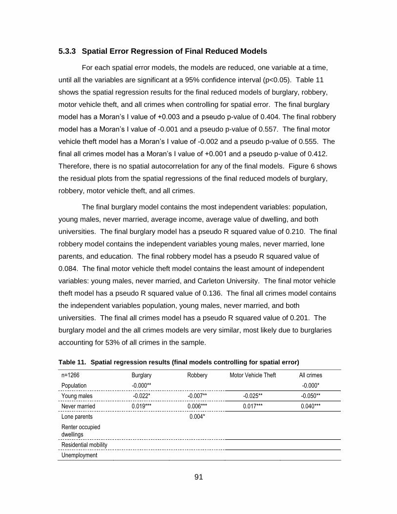
91
5.3.3 Spatial Error Regression of Final Reduced Models
For each spatial error models, the models are reduced, one variable at a time,
until all the variables are significant at a 95% confidence interval (p<0.05). Table 11
shows the spatial regression results for the final reduced models of burglary, robbery,
motor vehicle theft, and all crimes when controlling for spatial error. The final burglary
model has a Moran’s I value of +0.003 and a pseudo p-value of 0.404. The final robbery
model has a Moran’s I value of -0.001 and a pseudo p-value of 0.557. The final motor
vehicle theft model has a Moran’s I value of -0.002 and a pseudo p-value of 0.555. The
final all crimes model has a Moran’s I value of +0.001 and a pseudo p-value of 0.412.
Therefore, there is no spatial autocorrelation for any of the final models. Figure 6 shows
the residual plots from the spatial regressions of the final reduced models of burglary,
robbery, motor vehicle theft, and all crimes.
The final burglary model contains the most independent variables: population,
young males, never married, average income, average value of dwelling, and both
universities. The final burglary model has a pseudo R squared value of 0.210. The final
robbery model contains the independent variables young males, never married, lone
parents, and education. The final robbery model has a pseudo R squared value of
0.084. The final motor vehicle theft model contains the least amount of independent
variables: young males, never married, and Carleton University. The final motor vehicle
theft model has a pseudo R squared value of 0.136. The final all crimes model contains
the independent variables population, young males, never married, and both
universities. The final all crimes model has a pseudo R squared value of 0.201. The
burglary model and the all crimes models are very similar, most likely due to burglaries
accounting for 53% of all crimes in the sample.
Table 11. Spatial regression results (final models controlling for spatial error)
n=1266 Burglary Robbery Motor Vehicle Theft All crimes
Population -0.000**
-0.000*
Young males -0.022* -0.007** -0.025** -0.050**
Never married 0.019*** 0.006*** 0.017*** 0.040***
Lone parents
0.004*
Renter occupied dwellings
Residential mobility
Unemployment
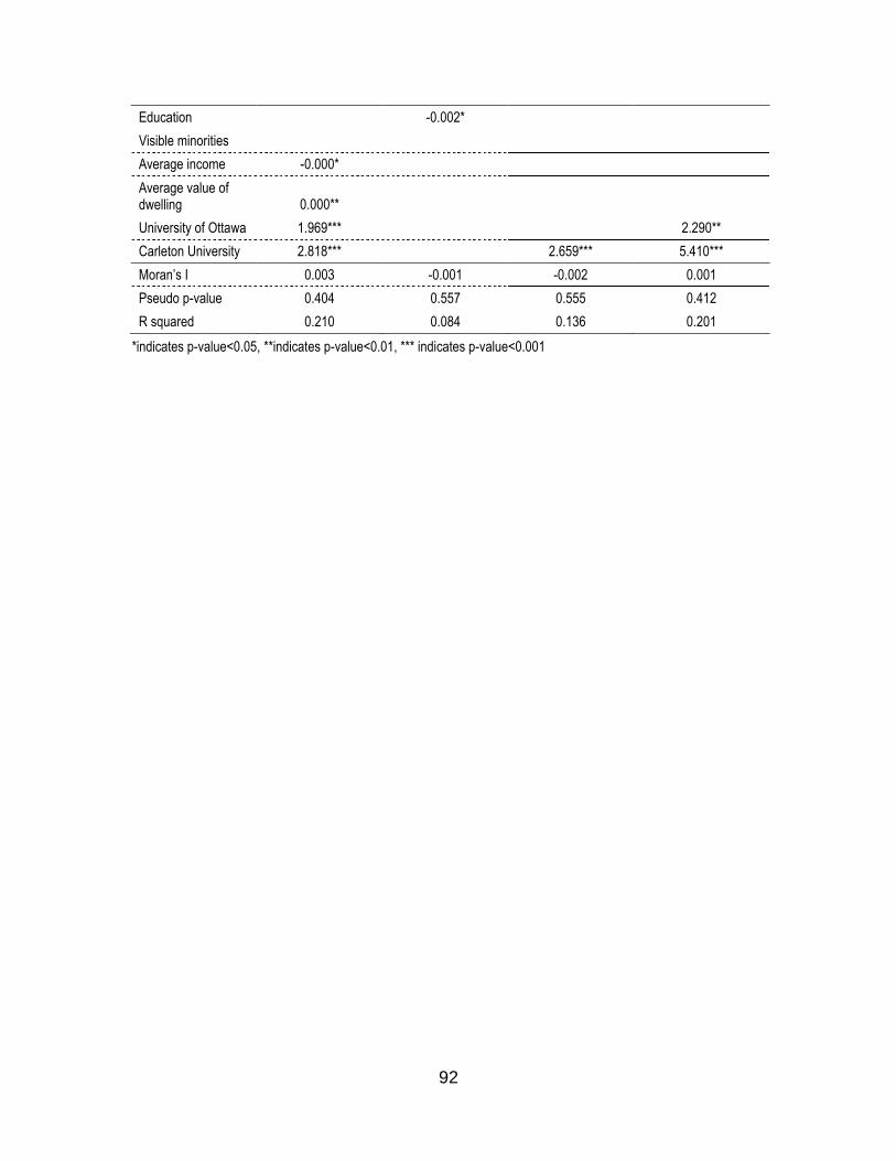
92
Education
-0.002*
Visible minorities
Average income -0.000*
Average value of dwelling 0.000**
University of Ottawa 1.969***
2.290**
Carleton University 2.818***
2.659*** 5.410***
Moran’s I 0.003 -0.001 -0.002 0.001
Pseudo p-value 0.404 0.557 0.555 0.412
R squared 0.210 0.084 0.136 0.201
*indicates p-value<0.05, **indicates p-value<0.01, *** indicates p-value<0.001

93
Figure 6. Residual plots for spatial regression (final models controlling for spatial error)
a. Burglary b. Robbery
c. Motor Vehicle Theft d. All Crimes
The presence of universities is significant in three of the four the models. Both
universities are significant in two models, burglary and all crimes. Only Carleton
University is significant in the motor vehicle theft model. Neither university is significant
in the robbery model. Renter occupied dwelling, residential mobility, unemployment, and
visible minorities are not significant and not included in any of the final models. This is
expected for renter occupied dwellings as it has a high correlation with never married
(r=0.743); therefore, never married would capture all of the variation between renter
occupied dwellings and the crime rates. Residential mobility has moderate correlations

94
with renter occupied dwellings (r=0.513) and never married (r=0.598). However, these
are not particularly high correlations, both less than 0.600. Unemployment and visible
minorities do not have any high correlations.
5.3.4 Crime Maps
Figure 7 through 10 are choropleth maps displaying the geographical
distributions of crime rates by dissemination area in Ottawa. The crime patterns for the
rates of each crime type show that, in general, crime tends to be highest in the
downtown core of the city and decreases as you move away from the city centre.
Figure 7. Ottawa burglary rate per 1,000 population by dissemination area (2006)
For burglary, the highest burglary rates are located in the downtown core of
Ottawa and just to the east and south of the downtown core. There are also high rates
of burglary in some of the dissemination areas immediately surrounding the city centre.
There are some medium rates of burglary in the dissemination areas in the southeast of
the city. The dissemination area containing the Carleton University has a high rate of
burglary (3.84). Of the five dissemination areas containing the University of Ottawa, two
have high rates of burglary (6.45 and 4.85), the former being the third highest rate of
burglary in the city, two have medium rates (3.41 and 2.23) and the other has a rate of
zero.

95
Figure 8. Ottawa robbery rate per 1,000 population by dissemination area (2006)
For robbery, there are a few clusters of robberies in the city centre of Ottawa,
with the highest rates of robbery located in the downtown core, but in fewer
dissemination areas. There are some medium rates of robberies in a few of the
dissemination areas outside of the city centre; however, the majority of the city has low
rates of robbery. The dissemination area containing the Carleton University has a low
rate of robbery (0.14). Of the five dissemination areas containing the University of
Ottawa, one has a high rate of robbery (1.39), the fifth highest rate in the city, one has a
low rate (0.19), and the others have a rate of zero.

96
Figure 9. Ottawa motor vehicle theft rate per 1,000 population by dissemination area (2006)
For motor vehicle theft, the highest rates of motor vehicle theft are also located in
the downtown core and just east of the downtown core. There are some medium rates
of motor vehicle theft in one or two dissemination areas as you move away from the city
centre to the south, west and east. The dissemination area containing the Carleton
University has a somewhat high rate of motor vehicle theft (3.27). Of the five
dissemination areas containing the University of Ottawa, two have medium rates of
motor vehicle theft (1.70 and 1.39) and the others have low rates (0.63, 0.56, and 0.20).

97
Figure 10. Ottawa all crimes rate per 1,000 population by dissemination area (2006)
For all crimes, the highest concentrations are located again in the city centre and
just to the east and south of the downtown core. There are high rates of all crimes in
some of the dissemination areas immediately surrounding the city centre and in a
dissemination area in the southwest. There are some medium rates of all crimes in the
dissemination areas just to southeast of the city centre. The dissemination area
containing the Carleton University has a somewhat high rate of burglary (7.24). Of the
five dissemination areas containing the University of Ottawa, one has a high rate of all
crimes (9.23), two have somewhat high rates (5.49 and 5.11), one has a medium rate
(2.97), and the other has a low rate (0.20).

98
6. Discussion
6.1. Findings
The visual observations of the choropleth maps of Ottawa show that crime is
highest in the city centre and decreases as you move away from the city centre; this was
true for each of the types of crime. This findings support the first hypothesis that there
are observable spatial patterns for burglary, robbery, motor vehicle theft, and all crimes
in Ottawa. Kitchen (2006) also found that crime in Ottawa is concentrated in the
downtown core of the city and decreases as you move towards the outer parts of the
city. This finding is in agreement with the ecological theories of Park and Burgess, and
supports Shaw and McKay’s social disorganization theory. It is also in agreement with
some of the literature reviewed that found that crime was concentrated in the city centre
(Malczewski & Poetz, 2005, 518; Nelson et al., 2001, 251).
The findings for the spatial regression models support the first and second
hypotheses. There are observable crime patterns for burglary, robbery, motor vehicle
theft, and all crimes. While there are some similarities in these patterns, there are also
differences in the spatial relationships for the different crime types. Overall, the final
models do not have high results for goodness of fit. Burglary has a pseudo R squared
value of 0.210, robbery has a pseudo R squared value of 0.084, motor vehicle theft has
a pseudo R squared value of 0.136 and all crimes has a pseudo R squared value of
0.201. The burglary model and the all crimes model have the best goodness of fit.
Therefore, the burglary rate and the total crime rate are better able to fit the data than
the rates of robbery rate or motor vehicle theft. Never married and young males are
significant for all of the crime types.
In the final regression model for burglary, population, young males, never
married, average income, average value of dwelling, and both universities are
significant. Burglary has negative relationships with population, young males, and
average income and positive relationships with never married, average value of dwelling,
and both universities. Dissemination areas with higher rates of burglary are

99
characterised with smaller populations, fewer young males, lower incomes, greater
proportion of people who have never been married and higher dwelling values.
In the final regression model for robbery, young males, never married, lone
parents, and education are significant. Robbery has negative relationships with young
males and education, and positive relationships with never married and lone parents.
Dissemination areas with higher rates of robbery are characterised with fewer young
males, lower education levels, and greater proportion of people who have never been
married and lone parents.
In the final regression model for motor vehicle theft, young males, never married,
and Carleton University are significant. Motor vehicle theft has a negative relationship
with young males and positive relationships with never married and Carleton University.
Dissemination areas with higher rates of motor vehicle theft are characterised with fewer
young males, and greater proportion of people who have never been married.
In the final regression model for all crimes, population, young males, never
married, and both universities are significant. The all crimes category has negative
relationships with population and young males, and positive relationships with never
married, and both universities. Dissemination areas with higher rates of all crimes are
characterised with smaller populations, fewer young males, lower incomes, greater
proportion of people who have never been married.
Never married has a positive relationship with all three crime types and all crimes
in general. This positive relationship is expected and supports routine activity theory.
The percentage of single people who have never been married in an area increases the
number of people who spend time in activities away from the home. This increases their
risk of personal victimization by increasing the potential of running into potential
offenders, including robbers, especially at night. It also increases their risk of property
victimization, as they leave their home unattended for longer amounts of time, which
increases the risk of burglary. This finding is consistent with some of the literature
examined as Dunn (1980a) found a positive relationship between never married and
robbery, Cohen and Cantor (1980) found a positive relationship between people who live
alone and the risk of robbery, and Kennedy and Forde (1990) found a positive
relationship between unmarried and burglary and robbery.

100
Young males have a negative relationship with all three crime types and all
crimes in general. This relationship is unexpected as, according to routine activity
theory, young males are expected to have a positive relationship with crime rates. The
percentage of young males in the population should represent the potential offenders in
the area, so an increase in young males should lead to an increase of crime. This
finding is inconsistent with the age-crime curve discussed previously. It is also
inconsistent with the literature, as Martin (2002) found a positive relationship between
young males and burglary, Fleming, Brantingham and Brantingham (1994) found a
positive relationship between motor vehicle theft and young males, and Andresen
(2006b) found a positive relationship between young males and both burglary and motor
vehicle theft. Cohen and Cantor (1980) found a positive relationship between age and
robbery, with the age group 16 to 29 years being the strongest predictor of personally
robbery. This result is especially notable as the presence of young males in the
population is consistently found in literature to be the most significant predictor of crime
rates in support of routine activity theory. A possible explanation for this finding might be
that the presence young males in the population are based on the residential population
rather than the ambient population. These results represent the influence of the
proportion of young males who live in the high crime areas rather than the proportion of
young males who frequent the high crime areas. As crime in Ottawa is concentrated in
the downtown core, the discrepancy between the characteristics of the ambient
population and the residential population is significant, and may influence crime patterns,
especially for the University of Ottawa that is located downtown.
The negative relationships between population and burglary and all crimes are
unexpected. According to routine activity theory and social disorganization theory, an
increase in population should increase crime by increasing the number of potential
offenders and targets in an area and decreasing the social cohesion in a neighbourhood.
This finding is inconsistent with some of the literature examined, as Cook (1983) found a
positive relationship between population and robbery. However, this finding is consistent
with Andresen’s (2006b) finding of a negative relationship between population and both
burglary and violent crime. Andresen also expected to see a positive relationship in
agreement with routine activity theory. Andresen suggested that this finding might have
been as result of the population providing guardianship rather than potential offenders
and targets (Andresen, 2006, 500). The use of an alternative measure of population
such as population density or ambient population may provide different results. Ambient

101
population may provide a better representation of the daytime distribution of potential
offenders and targets as most people leave their homes during the day (Andresen,
2006c, 273).
The negative relationship between burglary and average income is expected and
supports social disorganization theory. This relationship is not found in any of the other
crime types. Low socio-economic status and low income can impede participation in
formal social activities that can decrease formal and informal control and increase crime.
A number of studies found similar findings. Malczewski and Poetz (2005) and Martin
(2002) found negative relationships between burglary and average income. Similarly,
Ceccato, Haining and Signoretta (2002) found a positive relationship between burglary
and poverty. Andresen (2006b) found a positive relationship between average income
and burglary but not for other types of crime. However, this was a positive relationship,
not negative as found in this study, and supported routine activity theory, as an increase
in income may lead to an increase in valuable items to steal (Andresen, 2006b, 500).
The positive relationship between average value of dwelling and burglary is also
expected and supports routine activity theory. This relationship is also only found for
burglary. This demonstrates the importance of target attractiveness and suitability. The
higher the value of a dwelling, the more valuable it is as a target, with a greater potential
profit for the burglar. Areas with higher value dwellings are relatively more attractive
than areas with lower value dwellings. The other types of crime, robbery and motor
vehicle theft, would not have dwellings as the targets, so the value of dwellings would
not have as great an impact on the risk of those types of crime.
The positive relationship between lone parents and robbery is also expected and
supports social disorganization theory. This finding also supports routine activity theory.
However, this relationship is not found in any of the other crime types. According to
social disorganization theory, areas with higher proportions of lone parent households
have less informal social controls, which can lead to an increase in crime. Routine
activity theory agrees that lone parent households have less guardianship that can lead
to an increase in crime. This finding is in agreement with the literature examined. Smith
et al. (2000) and Kennedy and Forde (1990) both found a positive relationship between
robbery and lone parents. Andresen (2006b) found different results from this study. He
found a positive relationship between lone parents and burglary but a negative
relationship between lone parents and violent crime, which included robbery along with

102
assault, sexual assault, homicide, and other violent offences (Andresen, 2006b, 497-
498). However, Andresen’s result was unexpected in the context of social
disorganization theory and may have been due to the aggregated violent crime type
(Andresen, 2006b, 497-498).
Finally, the negative relationship between education and robbery is also
expected and supports social disorganization theory. Again, this relationship is found
only for robbery. Education is a protective factor in crime, as it provides informal control
and promotes social cohesion. Areas characterised by higher socio-economic status
and higher levels of education experience less robbery due to a greater amount of
informal control and social cohesion in those areas. This finding is in agreement with
some of the literature reviewed. Cahill and Mulligan (2003) found that low socio-
economic status and low education was a strong indicator of crime.
There are no relationships found for renter occupied dwellings, residential
mobility, unemployment, and visible minorities in the final regression models. This is
unexpected and does not support social disorganization theory. All of these variables
are expected to have a positive relationship with crime. This lack of relationship is also
inconsistent with the literature, as many studies have found that unemployment is one of
the greatest predictor of crime rates (Andresen, 2006c, 269; Andresen, 2006b, 49;
Cohen & Cantor, 1980, 153; Kennedy & Forde, 1990, 145-146).
These findings support the third hypothesis that there are spatial relationships
between the socio-demographic and socio-economic characteristics of a neighbourhood
and the crime rates. However, these relationships vary by the type of crime. Never
married and young males are related to all three crime types. In addition to these two
variables, burglary is also related to population and average income. Robbery is related
to lone parents and education in addition to the two common variables. However, motor
vehicle theft is only related to those two variables. All crimes are related to the two
common variables and population.
In general, the results of the spatial regression analysis support both social
disorganization theory and routine activity theory, although some of the results are
unexpected and do not support the theories. Many of the findings are also consistent
with the relevant literature examined in this study. The positive relationship between
lone parents and robbery supports both social disorganization theory and routine activity
theory. The negative relationships between education and robbery and average income

103
and burglary support social disorganization theory. The positive relationships between
average value of dwelling and burglary and never married and all types of crimes
support routine activity theory. The findings that do not support these theories are the
negative relationship between population and burglary that are contrary to the results
expected by social disorganization theory, and the negative relationships between young
males and the three types of crime, which is contrary to the results expected by routine
activity theory. The lack of expected positive relationships between crime and visible
minorities, unemployment, renter occupied dwellings, and residential mobility fail to
support social disorganization theory.
The positive relationships between the presence of universities and crime
support the geometric theory of crime and crime pattern theory. Higher rates of crime
found in dissemination areas containing a university could suggest that the universities
are influencing the amount of crime in the dissemination area. The university nodes may
be acting as crime generators, drawing potential offenders and targets to the campus for
activities resulting in the campus becoming a part of their awareness space and
increasing the potential for a criminal event to occur. As more criminals become aware
of the potential opportunities for crime on campus, the universities become crime
attractors. There may also be paths within these dissemination areas that frequented by
potential offenders and targets travelling to and from the university that are high crime
areas.
The University of Ottawa has positive relationships with burglary and all crimes,
while Carleton University has positive relationships with burglary, motor vehicle theft and
all crimes. This supports the fourth hypothesis that there are spatial relationship
between universities and the rate of burglary, motor vehicle theft and all crimes but not
robbery. The universities are also the strongest predictors in the models, with the
largest magnitude of the estimated coefficients in the burglary, motor vehicle theft, and
all crimes models. However, in the burglary and all crimes models, where both
universities are strong predictors of crime, Carleton University has the greater impact. In
the motor vehicle theft model, only Carleton University was significant. Carleton
University is located outside the city centre while the University of Ottawa is located
downtown. Carleton University may have more students and staff commuting to the
campus by vehicle, creating more opportunities for motor vehicle theft in the parking lots
on Carleton’s campus.
104
The lack of relationship between robbery and the universities is a positive result;
significant relationships are only found for the property crimes, burglary and motor
vehicle theft. This finding might suggest that personal victimization is not an issue on
campuses in Ottawa. However, other violent crimes such as assault would need to be
examined in order to reach this conclusion. Alternatively, the lack of relationship may
simply be the result of the smaller number of robbery offences included the sample, as
robbery tends to be a more rare occurrence than property offences.
6.2. Limitations
The unit of analysis of this study may be a limitation of the data and should be
taken into account when interpreting the results of this study. The ecological fallacy,
discussed previously in this study, states that the inappropriate inference from one
spatial unit of analysis to reach conclusions about another level of spatial unit can lead
to meaningless conclusions (Brantingham & Brantingham, 1984, 228). Similarly, the
modifiable areal unit problem, also discussed previously, states that there are multiple
ways in which data can be aggregated and that studying the wrong unit of analysis can
lead to misleading interpretation of results (Weisburd et al., 2009, 19). Spatial patterns
can differ depending on the unit of analysis and the aggregation of data can hide within
unit variation that is visible at lower levels of analysis (Brantingham &Brantingham, 1981,
22). These potential sources of error could affect the results of the analysis.
Some studies examined the differences in results when crime data are
aggregated to various levels of analysis. Andresen and Malleson (2011) found that
general crime patterns are somewhat similar at different spatial levels, but the finer
scales show significant variation within the larger units (Andresen & Malleson, 2011, 72).
Street segments made better units of analysis than the dissemination area and census
tract units of analysis, as the ecological fallacy influences findings when data are
aggregated to the dissemination area and census tract levels (Andresen & Malleson,
2011, 72). Andresen and Linning (2012) found that aggregation to the census tract and
dissemination area level is only justifiable for robbery crime types in Ottawa (Andresen &
Linning, 2012, 279). Kitchen (2006) found increased significance in the strength of the
relationships between several socio-demographic indicators and crime at the
neighbourhood level in comparison to the dissemination area level in Ottawa (Kitchen,
2006, 85).

105
Alternatively, Ceccato, Haining and Signoretta (2002) found that aggregating
data into larger areas increased the base population of each area, allowing crime rates
to be calculated from larger denominators and resulting in more robust within-area
variation in the number of cases than may be due to random variation (Ceccato, Haining
& Signoretta, 2002, 37). It also reduced the effects of any inaccuracies in the data or
inaccuracies in the location of offences due to geocoding errors (Ceccato, Haining &
Signoretta, 2002, 37). Craglia et al. (2000) agreed that random error was often smaller in
aggregated data as the differences are averaged out (Craglia et al., 2000, 720). Smaller
units of analysis are more impacted by the interdependence of adjacent and nearby
areas and need to pay more attention to the interactions between adjacent and nearby
areas (Weisburd et al., 2009, 24).
Rengert and Lockwood (2009) identified common problems that could arise when
aggregating crime data. The first problem is associated with using political boundaries
not created for research purposes, as these do not represent conceptual
neighbourhoods or populations (Rengert & Lockwood, 2009, 111). This could be a
potential source of error, as dissemination areas may not accurately represent the
neighbourhood as perceived by residents in Ottawa. The second problem is the effect of
edges and boundaries that may cause a researcher to miss clusters of crimes between
areas (Rengert & Lockwood, 2009, 112). This study attempts to account for this by
testing for spatial autocorrelation and controlling for spatial dependence. The last
problem is as the unit of analysis becomes larger, it becomes more likely that two or
more variables will be significantly related because the variance in the data decreases
as the level of aggregation increases (Rengert & Lockwood, 2009, 116). To account for
this, some studies have used multiple levels of spatial units in the analysis in order to
determine whether the aggregation level used in the study could result in biased findings
(Rengert & Lockwood, 2009, 109). This might be beneficial and could be a suggestion
for future research.
The ideal unit of analysis for studying the crime pattern theory would be at the
address level. However, the analysis of the crime data in this study is dependent on the
unit of analysis available for census data. As the dissemination area is the smallest unit
available for census data, this measure is better than other census units. Another
advantage is that dissemination areas follow roads and other boundaries of the physical
environment that people also tend to follow in their movements. There may be a

106
quantitative change in the results, such as an increase or decrease in the significance or
magnitude of the statistical tests based on the choice of the unit of analysis (Andresen,
2009, 334-335).
The reliability and validity of officially collected crime data as a measure of the
actual occurrence of crime has been questioned due to problems such as the dark figure
of crime and potential biases in policing practices and decision making discussed
previously in this study. There can be spatial biases in the patterns of official crime data
as police may pay attention to some areas more than others or the residents of some
areas may be less willing to report crime to police than other areas (Brantingham &
Brantingham, 1981, 24).
This study uses weekly police activity reports that are police reported crime data.
A limitation of weekly activity reports is the data represent the number of crimes that
have come to the attention of the police. This may reflect biases in official reactions to
crime and levels of policing rather than actual levels of crime. It also relies on the
accuracy of police recoding incidents of crime and the related spatial information.
However, weekly crime reports are not subject to some of the limitations found in other
official crime measures such as Uniform Crime Reports or calls for police service,
discussed previously in this study. Weekly activity reports are not subject to the most
serious offence rule or multiple reports of same incident that unsubstantiated by the
police. Weekly police activity reports are also not subject to some of the limitation of
victimization surveys which require large sample sizes to be spatially representative of
the of small areas within a city.
The geocoding of the weekly crime reports had a hit rate of 92.5%. While this hit
rate was above Ratcliffe’s minimum acceptable hit rate, some of the cases were not
geocoded. If there are spatial biases in the geocoding misses, this could result in biased
spatial patterns. One potential limitation of the geocoding is the By Ward Market area.
As discussed previously, crimes located in By Ward Market did not have a matching
street name for geocoding and could not be geocoded. As By Ward Market is a
population node for entertainment and shopping activities, this could affect the results of
the analysis if many crimes occur in this area. However, upon inspection of the dataset,
By Ward Market was the location of only five crimes. Therefore, this likely did not affect
the results. In addition, Kitchen (2006) found that By Ward Market was a high crime

107
area for violent crime, particularly threats and assaults, crime types not included in this
analysis.
Another potential limitation of the data in this study is the denominator used to
calculate crime rates. The bases selected for calculating crime rates can influence the
results, as they may not represent the spatial distribution of potential targets
(Brantingham & Brantingham, 1981, 24). The residential population is the denominator
used to calculate the crime rate for each crime type. The residential population is
included in the census data and is the most common measured used to calculate crime
rates. However, the residential population denominator has some limitations. The
residential population may not represent the distribution of targets within space, as the
residential population is a measure of where the population lives, not where they spend
their time. This is especially problematic in central business districts where the majority
of people travel from surrounding areas to visit or work and for crimes where the targets
are mobile. Using the residential population in these cases can lead to artificially high
offence rates (Bottoms & Wiles, 2002, 626). This may have influenced the patterns
observed in the crime maps.
There are alternative measures that can be used to calculate crime rates. The
ambient population, as discussed previously, is an estimate of the daytime population to
reflect the travel patterns and distribution of population in the city centre during the day.
Andresen (2011b) found similar correlations between the resident and ambient based
violent crime rates at the census tract level but very different correlations at the
dissemination area level (Andresen, 2011b, 200-2001). However, ambient population
does represent the distribution of targets for all types of offences. Opportunity based
crime rates use crime specific denominators to reflect the targets at risk rather than to a
population base (Harries, 1981, 148-149). Opportunity based crime rates include
number of dwellings to represent burglary targets, number of vehicles to represent motor
vehicle theft targets and ambient population to represent robbery targets. However,
opportunity based crime rates would pose a problem when calculating the total crime
rate for all types of crime, as a single measure would need to reflect all crimes.
Residential population also works for burglary crime rates as the targets of burglaries are
often homes where people live. Using ambient-based crime rates or opportunity based
crime rates may lead to different results. As residential population is the denominator for
all crime types in this study, it is a limitation, which must be taken into consideration in

108
the interpretation of the results. Future studies could use different denominators to
calculate the rate for each type of crime.
There are a number of decisions made in the operationalization of the
independent variables that may influence the results and therefore are possible
limitations of this study. The independent variables for the two universities are
calculated using a spatial containment process that indicates whether the dissemination
area, or any portion of the dissemination area, contains the university. For both
universities, this spatial containment process is based on the main campus. However,
the University of Ottawa has other campuses located around the city of Ottawa. As
these were only small campuses for specific departments or schools within the
university, they are not included in the analysis. However, this may affect the results, as
these smaller campuses may also be activity nodes that attract crime and should be
considered as a limitation of the study.
Carleton University is contained within a single dissemination area.
Unfortunately, this dissemination area did not have complete census data. Therefore,
the census data had to be approximated by taking the average value of the surrounding
dissemination areas. Some of the census variables did have data for this dissemination
area so these variables were to examine the accuracy of the other census estimates for
this dissemination area. As discussed previously, the actual census values for this
dissemination area and the estimated values are very similar; therefore, it is believed
that the estimation for this dissemination area is a good approximation of the actual
values for the missing census data. However, this should still be considered a limitation
of the data used in this study. Another limitation of the census data is the sampling error
and random rounding which resulted in renter occupied dwellings and visible minorities
with greater than 100% in a dissemination area. This may affect results and is a
limitation of the data in this study. Future studies may consider aggregating the data to
a larger unit of analysis to minimize the affect of sampling error and random rounding.
There are a number of alternative measures that could have been used to
represent the socio-economic and socio-demographic variables from the census data.
The population density, rather than the total population of an area, could population.
The variable for young men could be calculated as the percentage of males 15 to 24
years rather than 15 to 29 years. Residential mobility could be measured by the
percentage of movers within one year rather than five years. The percentage of recent
109
immigrants could represent ethnic heterogeneity rather than measuring racial
heterogeneity by the percentage of visible minorities in the population. The average
family income could represent income rather than the average income of population 15
years of older. The percentage of female-headed households with children could
represent family disruption rather than lone parent households. All these alternative
ways of measuring the socio-demographic characteristics of the population might result
in different relationships. Future studies may consider using these alternative measures.
Spatial regression works poorly with crime rates when there is zero population in
an area, as the crime rate in those areas would be infinity. Therefore, the dissemination
areas with a population of zero were eliminated from this study. However, this removes
the geography upon which the technique is based (Kamber et al., 2000, 116). Spatial
regression does not work well with discontinuous distributions (Kamber et al, 2000, 118).
This is a limitation of the data analysis conducted in this study. Nine dissemination
areas (4% of the sample) did not have population data available; these dissemination
areas were removed from the analysis. These dissemination areas are not clustered in
one area of the city and should not bias the spatial distribution of one area. Future
studies could retain the dissemination areas with populations of zero and use a different
method of analysis to address this limitation.
There is another limitation to using crime rates in conducting spatial regression
analysis. Moran’s I is highly sensitive to the unit of analysis (Kamber et al., 2000, 115).
Crime rates have different variances when the denominator is not constant that can lead
to spurious indications of spatial autocorrelation (Anselin, Griffiths & Tita, 2008, 112).
This can be corrected by using an Empirical Bayes approach in GeoDa 0.9.5-i to
standardise each rate used in calculation of Moran’s I (Anselin, Griffiths & Tita, 2008,
112). However, this was not done in this study. This would be a suggestion for future
research.
6.3. Implications
The finding of spatial autocorrelation amongst the variables in this study
demonstrates the importance of spatial neighbours in the spatial analysis of crime.
Crime places should not be considered in isolation of the surrounding areas. This is
important for the implementation of policy or crime prevention initiatives. As stated by
Andresen, “the relationship between places are important for understanding crime

110
across places” (Andresen, 2011a, 401). Crime prevention policies should take into
consideration the influence of the characteristics of surrounding neighbourhoods when
developing solutions to crime problems in a particular area, as well as the effect the
characteristics of the target area will have on the surrounding neighbourhoods. The
edges or boundaries between areas may also be influencing the crime patterns.
The findings of the spatial regression models demonstrate the importance the
relationship between universities and crime. Universities may act as crime attractors
and increase crime in these areas. Universities can take steps to implement crime
reduction policies in attempt to decrease criminogenic factors on campus, such as
increased lighting and security, and restrictions on student drinking and parties on
campus. The significance of the never married population in the final models for all
crime types demonstrates the need for greater levels of guardianship on campuses or in
the surrounding areas as the residents spend more time away from home. It is possible
that the relationship observed between motor vehicle theft and Carleton University but
not the University of Ottawa could be due to students commuting to the Carleton
University campus, as it is further outside the city centre than the University of Ottawa.
The number of vehicles in the parking lots on campus may be the cause of this
relationship. In this case, the campus could increase security in the parking lots.
A suggestion for future research would include the use of multiple levels of
spatial units in the analysis. Andresen and Malleson (2011) and Andresen and Linning
(2012) compared multiple levels of analysis in order to determine the resulting
differences in crime patterns. Some other units of analysis that could be useful to
include are street segments or census tracts. Further research on this topic would be
helpful in determining the impact of each unit of analysis on the spatial patterns of crime.
Including other spatial levels of analysis may confirm the results found in this study and
provide greater insight into the observed results.
Another suggestion for future research would include the use of multiple
denominators for calculating the crime rates. Andresen (2006c) and Andresen (2011c)
examined the difference in results when using residential population and ambient
population as the denominator for crime rates. However, future studies could
incorporate a variety of opportunity based crime rates as well. This would be helpful to
determine the impact of the different denominators on the spatial patterns of crime.

111
Other variables available in the census data could have been included in the
models. Housing structure characteristics such as the number of dwellings in an area,
the age of construction of dwellings, and the type of dwellings, including apartment
buildings, row houses, and private residences could be included in the models. Future
studies could incorporate these variables in their analysis to determine whether the
addition of these variables would have resulted in different conclusions.
Some alternative methods could have been used in the spatial regression
analysis. This study removed the dissemination areas for which the population was
zero. Future studies could retain the dissemination areas with populations of zero and
use a different method of analysis to address this limitation. Future studies could also
correct for the limitation of using crime rates in spatial regression analysis by using an
Empirical Bayes approach.
Other suggestions for future research would be to include the presence of other
nodes, such as shopping centres, entertainment districts and central business districts,
in the analysis. These nodes could act as crime attractors and generators, influencing
crime patters. Temporal patterns could be examined to determine whether the observed
results occur at different time such as during the day or evening. Finally, the spatial
regression analysis could be conducted for many other Canadian cities to determine
whether the results observed in Ottawa are also found in other cities, or if they are
unique to Ottawa.
6.4. Conclusion
This study examined the influence of universities, as well as other socio-
demographic characteristics, on the crime patterns of burglary, robbery, and motor
vehicle theft in Ottawa. Crime pattern theory, that incorporates aspects and routine
activity theory, the geometric theory of crime, and social disorganization theory, was the
theoretical framework used to examine the geographic distribution of these factors on
crime patterns. A spatial autocorrelation and spatial regression analysis was conducted
on models for each crime type. There were some interesting relationships found in this
analysis.
The results of this study were somewhat consistent with the theoretical
expectations of routine activity theory and social disorganization theory. The positive
relationship observed between lone parents and robbery supported both social

112
disorganization theory and routine activity theory, as areas higher in lone parent
households tend to have higher rates of robbery, due to decreased informal controls and
guardianship. The negative relationships found between education and robbery and
average income and burglary supported social disorganization theory, as areas
characterised by lower levels of education and income tend to have higher crime rates
due to the lower socio-economic status of the population in the area and the lack of
social cohesion. The positive relationships observed between average value of dwelling
and burglary and never married and all types of crimes supported routine activity theory.
Areas characterised by higher property values provide attractive targets for burglary
offenders and a large percentage of single people in an area provides more targets
without capable guardians, which creates opportunities for crime in general. However, a
number of the expected relationships in support of social disorganization theory were not
observed, and the finding for young males contrary to the expected findings did not
support routine activity theory. The results of this study also supported the integration of
routine activity theory and social disorganization theory as the use of only one of these
theories would have reduced the predictive power of the models.
The results of this study did support the crime pattern theory. The positive
relationships between the universities and crime demonstrated that the universities could
be acting as crime attractors, for certain types of crime, by drawing potential offenders
and targets to the campus and increasing the potential for a criminal event to occur.
Carleton University was related to all types of crime expect for robbery, while the
University of Ottawa was only related to burglary and all crimes. This suggests there
could be geographical differences between the two campuses influencing the crime
patterns.

113
Reference List
Ackerman, W. V., & Murray, A. T. (2004). Assessing spatial patterns of crime in Lima, Ohio [Electronic version]. Cities, 21(5), 423-437. Retrieved September 25, 2009 from Academic Search Premier.
Andresen, M. A. (2006a). A procedure for geocoding point addresses using ArcView GIS 3.x [Electronic version]. Burnaby, BC: Institute for Canadian Urban Research Studies. Retrieved January 21, 2012 from http://www.sfu.ca/~andresen/papers/Geocoding_Procedure_ArcView.pdf.
Andresen, M. A. (2006b). A spatial analysis of crime in Vancouver, British Columbia: A synthesis of social disorganization and routine activity theory [Electronic version]. The Canadian Geographer, 50(4), 487-502. Retrieved June 13, 2010 from Willey Online Library.
Andresen, M. A. (2006c). Crime measures and the spatial analysis of criminal activity [Electronic version]. British Journal of Criminology, 46, 258-285. Retrieved October 23, 2009 from Oxford Journals Online.
Andresen, M. A. (2007). Location quotients, ambient populations, and the spatial analysis of crime in Vancouver, Canada. Environment and Planning, 39, 2423-2444.
Andresen, M. A., (2009). Testing for similarity in area-based spatial patterns: A non-parametric Monte Carlo approach [Electronic version]. Applied Geography, 29, 333-345. Retrieved June 13, 2010 from Elsevier Science Direct.
Andresen, M. A. (2010). The place of environmental criminology within criminological though. In M. A. Andresen & J. B. Kinney (Eds.), Classics in environmental criminology (pp.5-28). Burnaby, BC: Simon Fraser University Publications.
Andresen, M. A. (2011a). Estimating the probability of local crime clusters: The impact of immediate spatial neighbours [Electronic version]. Journal of Criminal Justice, 39, 394-404. Retrieved December 20, 2012 from Elsevier Science Direct.
Andresen, M. A. (2011b). The ambient population and crime analysis [Electronic version]. The Professional Geographer, 63(2), 193-212. Retrieved December 21, 2012 from http://www.sfu.ca/content/dam/sfu/icurs/Publications/2011/Andresen_ambient%20pop.pdf.

114
Andresen, M. A., & Brantingham, P. L. (2008). Visualizing ambient population data within census boundaries: A dasymetric mapping procedure [Electronic version]. Cartographica, 43(4), 267-275. Retrieved June 13, 2010 from Academic Search Premier.
Andresen, M. A., & Kinney, J. B. (Eds.). (2012). Patterns, prevention, and geometry of crime. New York, NY: Routledge.
Andresen, M. A., & Linning, S. J. (2012). The (in)appropriateness of aggregating across crime types [Electronic version]. Applied Geography, 35, 275-282. Retrieved December 20, 2012 from Elsevier Science Direct.
Andresen, M. A., & Malleson, N. (2011). Testing the stability of crime patterns: Implications for theory and policy [Electronic version]. Journal of Research in Crime and Delinquency, 48(1), 58-62. Retrieved December 20, 2012 from Sage Premier Online.
Andresen, M. A., Wuschke, K., Kinney, J. B., Brantingham, P. J., & Brantingham, P. L. (2009). Cartograms, crime, and location quotients [Electronic version]. Crime Patterns and Analysis, 2(1), 31-46. Retrieved May 16, 2010 from http://www.eccajournal.org/V2N1S2009/Andresen.pdf.
Anselin, L. (2003a). An introduction to EDA with GeoDa [Electronic version]. Retrieved October 3, 2010 from http://geodacenter.asu.edu/system/files/quicktour.pdf.
Anselin, L. (2003b). An introduction to spatial autocorrelation analysis with GeoDa [Electronic version]. Retrieved October 3, 2010 from http://geodacenter.asu.edu/system/files/spauto_0.pdf
Anselin, L. (2005). Exploring spatial data with GeoDa: A workbook [Electronic version]. Retrieved October 3, 2010 from http://geodacenter.asu.edu.
Anselin, L., Griffiths, E., & Tita, G. (2008). Crime mapping and hot spot analysis. In R. Wortley & L. Mazerolle (Eds.), Environmental criminology and crime analysis (pp. 97-115). Portland, Oregon: Willan Publishing.
Anselin, L., Syabri, I., & Kho, Y. (2006). GeoDa: An introduction to spatial data analysis [Electronic version]. Geographical Analysis, 38, 5-22. Retrieved August 14, 2010 from Wiley Online Library.
Bernasco, W., & Block, R. (2011). Robberies in Chicago: A block-level analysis of the influence of crime generators, crime attractors, and offender anchor points [Electronic version]. Journal of Research in Crime and Delinquency, 48, 33-57. Retrieved March 26, 2012 from Sage Premier Online.
Block, R. L., & Block, C. R. (1995). Space, place and crime: Hot spot area and hot places of liquor-related crime. In Crime prevention studies: Vol. 4. Crime and place (pp.145-183) [Electronic version]. Monsey: New York: Criminal Justice Press. Retrieved August 26, 2010 from http://www.popcenter.org/library/crimeprevention/volume_04/.

115
Block, R. L., & Block, C. R. (2000). The Bronx and Chicago: Street robbery in the environs of rapid transit stations. In V. Goldsmith, P.G. McGuire, J.H. Mollenkopf & T.A. Ross (Eds.), Analyzing crime patterns: Frontiers of practice. (pp. 137-152). Thousand Oaks, California: Sage Publications Inc.
Boba, R. (2005). Crime analysis and crime mapping. Thousand Oaks, CA: Sage Publications Inc.
Booth, A., Johnson, D. R., & Choldin, H. M. (1977). Correlates of city crime rates: Victimization surveys versus official statistics [Electronic version]. Social Problems, 25(2), 187-197. Retrieved March 27, 2009 from JSTOR database.
Bottoms, A. E. (2007). Place, space, crime, and disorder. In M. Maguire, R. Morgan, R. Reiner (Eds.), The Oxford handbook of criminology (4th ed.). (pp. 528-574).Oxford: UK: Oxford University Press.
Bottoms, A. E., & Wiles, P. (2002). Environmental criminology. In M. Maguire, R. Morgan, & R. Reiner (Eds.), The Oxford handbook of criminology (3rd ed.). (pp. 620-652). Oxford, UK: Oxford University Press.
Bowers, K. J., & Johnson, S. D., & Pease, K. (2005). Victimisation and re-victimisation risk, housing type, and area: A study of interactions [Electronic version]. Crime Prevention and Community Safety: An International Journal, 7(1), 7-17. Retrieved February 12, 2008 from Business Source Complete.
Brantingham, P. J., & Brantingham, P. L. (1978). A theoretical model of crime site selection. In M. D. Krohn & R. L. Akers (Eds.), Crime, law, and sanction: Theoretical perspectives (pp.105-117). Beverly Hills, California: Sage Publication Inc.
Brantingham, P. J., & Brantingham, P. L. (Eds.). (1981). Environmental criminology. Beverly Hills, California: Sage Publication Inc.
Brantingham, P. J., & Brantingham, P. L. (1984). Patterns in crime. New York, NY: Macmillian Publishing Company.
Brantingham, P. L., & Brantingham, P. J. (1975). Residential burglary and urban form [Electronic version]. Urban Studies, 12(3), 273-284. Retrieved February 12, 2008 from Informaworld.
Brantingham, P. L., & Brantingham, P. J. (1993a). Nodes, paths and edges: Considerations on the complexity of crime and the physical environment [Electronic version]. Journal of Environmental Psychology, 13, 3-28. Retrieved May 3, 2007 from JSTOR database.
Brantingham, P. L., & Branthingham, P. J. (1993b). Environment, routine, and situation: Towards a pattern theory of crime. In F. Adler & W. Laufer (Series Eds.) & R. V. Clarke & M. Felson, (Vol. Eds.), Advances in criminological theory: Vol. 5. Routine activity and rational choice. (pp. 259-287). New Brunswick, NJ: Transaction Publishers.

116
Brantingham, P., & Brantingham, P. (2008). Crime pattern theory. In R. Wortley & L. Mazerolle (Eds.), Environmental criminology and crime analysis (pp. 78-91). Portland, Oregon: Willan Publishing.
Brantingham, P. J., Dyreson, D. A., & Brantingham, P. L. (1976). Crime seen through a cone of resolution [Electronic version]. American Behavioral Scientist, 20(2), 261-273. Retrieved June 13, 2010 from Sage Premier Online.
Brantingham, P. L., Brantingham, P. J., Vajihollahi, M., & Wuschke, K. (2009). Crime analysis at multiple scales of aggregation: A topological approach. In D. Weisburd, W. Bernasco, & Bruinsma, G. J. N. (Eds.), Putting crime in its place: Units of analysis in geographic criminology (pp. 87-107) [Electronic version]. New York, NY: Springer Science and Business Media. Retrieved August 26, 2010 from Springer Link Online.
Bromley, M. L. (1995). Factors associated with college crimes: Implications for campus police [Electronic version]. Journal of Police and Criminal Psychology, 10(3), 13-19. Retrieved December 20, 2012 from Springer Link Online.
Brower, A. M., & Carroll, L. (2007). Spatial and temporal aspects of alcohol-related crime in a college town [Electronic version]. Journal of American College Health, 55(5), 267-275. Retrieved December 21, 2012 from Taylor & Francis Online.
Bruce, C. W., Hick, S. R., & Cooper, J. P. (Eds.). (2004). Exploring crime analysis: Readings on essential skills. Overland Park, KS: International Association of Crime Analysts.
Buerger, M. E., Cohn, E. G., & Petrosino, A. J. (1995). Defining the “hot spots of crime”: Operationalizing theoretical concepts for field research [Electronic version]. In J.E. Eck & D. Weisburd (Eds.), Crime and place (pp. 237-258). Monsey, NY: Criminal Justice Press. Retrieved May 16, 2010 from http://www.popcenter.org/library/crimeprevention/volume_04/11-Buerger.pdf.
Bunge, V. P., Johnson, H., & Balde, T. A. (2005). Exploring crime patterns in Canada [Electronic version]. Crime and justice research paper series (Catalogue no. 85-561-MIE No. 005). Ottawa, Ontario: Statistics Canada. Retrieved March 27, 2009 from http://publications.gc.ca/Collection/Statcan/85-561-MIE/85-561-MIE2005005.pdf?.
Cahill, M., & Mulligan, G. F. (2003). The determinants of crime in Tuscon, Arizona [Electronic version]. Urban Geography, 24(7), 582-610. Retrieved August 15, 2010 from Meta Press.
Canter, P. R. (1998). Geographic information system and crime analysis in Baltimore County, Maryland. In J. Eck & D. Weisburd (Eds.), Crime prevention studies: Vol. 8. Crime mapping and crime prevention (pp. 158-190) [Electronic version]. Monsey: New York: Criminal Justice Press Retrieved August 26, 2010 from http://www.popcenter.org/library/crimeprevention/volume_08/.
Carleton University. (2011). About Carleton. Retrieved March 26, 2012 from Carleton University’s website: http://www1.carleton.ca/about/.
117
Ceccato, V., Haining, R., & Signoretta, P. (2002). Exploring offence statistics in Stockholm city using spatial analysis tools [Electronic version]. Annals of the Association of American Geographers, 92(1), 29-51. Retrieved September 25, 2009 from Academic Search Premier.
Ceccato, V., & Oberwittler, D. (2008). Comparing spatial patterns of robbery: Evidence from a western and an eastern European city [Electronic version]. Cities, 25, 185-196. Retrieved September 25, 2009 from Academic Search Premier.
Clare, J., Fernandez, J., & Morgan, F. (2009). Formal evaluation of the impact of barriers and connectors on residential burglars’ macro-level offending location choices [Electronic version]. The Australian and New Zealand Journal of Criminology, 42(2), 139-158. Retrieved May 11, 2010 from Sage Premier Online.
Clarke, R. V., & Mayhew, P. (1994). Parking patterns and car theft risks: Policy-relevant findings from the British crime survey. In R. V. Clarke (Ed.), Crime prevention studies: Vol. 3. (pp. 91-107). [Electronic version]. Monsey: New York: Criminal Justice Press. Retrieved August 26, 2010 from http://www.popcenter.org/library/crimeprevention/volume_03/.
Cohen, L. E., & Cantor, D. (1980). The determinants of larceny: An empirical and theoretical study [Electronic version]. Journal of Research in Crime and Delinquency, 17, 140-159. Retrieved August 21, 2010 from Sage Premier Online.
Cohen, L. E., & Felson, M. (1979). Social change and crime rate trends: A routines activity approach [Electronic version]. American Sociological Review, 44(4), 588-608. Retrieved March 27, 2009 from JSTOR database.
Cohen, L. E., & Land, K. C. (1984). Discrepancies between crime reports and crime surveys: Urban and structural determinants [Electronic version]. Criminology, 22(4), 499-530. Retrieved March 27, 2009 from Wiley Online Library.
Community Foundation of Ottawa. (2007). Ottawa’s vital signs report 2007. Retrieved March 28, 2010 from http://www.communityfoundationottawa.ca/site/site_en/programs/documents/Otta wa%20Vital%20Signs%20-%202007.pdf
Cook, P. J. (1983). Robbery in the United States: An analysis of recent trends and patterns. Washington, DC: US Department of Justice National Institute of Justice.
Craglia, M., Haining, R., & Wiles, P. (2000). A comparative evaluation of approaches to urban crime pattern analysis [Electronic version]. Urban Studies, 37(4), 711-729. Retrieved March 27, 2009 from Academic Search Premier.
Daday, J. K., Broidy, L. M., Crandall, C. S., & Sklar, D. P. (2005). Individual, neighborhood, and situational factors associated with violent victimization and offending [Electronic version]. Criminal Justice Studies, 18(3), 215-235. Retrieved May 11, 2010 from Taylor & Francis Online.
Decker, D. L., Shichor, D., & O’Brien, R. M. (Eds.). (1982). Urban structure and victimization. Toronto: Lexington Books.

118
Dunn, C. S. (1980a). Crime area research. In D. E. Georges-Abeyie & K. D. Harries (Eds.), Crime: A spatial perspective (pp. 5-23). New York, NY: Columbia University Press.
Dwyer, M. (2006, Nov. 13). Our 16th annual rankings. Maclean’s Magazine, 119(45), 74-79. Retrieved December 31, 2012 from http://www.macleans.ca/education/universities/article.jsp?content=20061113_136532_136532
Eck, J.E., & Weisburd, D. (Eds.). (1995). Crime places in crime theory. In Crime and place (pp.1-33) [Electronic version]. Monsey: New York: Criminal Justice Press. Retrieved March 28, 2007 from Proquest CSA LLC reference.
Einstadter, W. J., & Henry, S. (Eds.). (2006). Criminological theory: An analysis of its underlying assumptions (2nd ed.). Lanham, Maryland: Rowman & Littlefield Publishers Inc.
Engstad, P. A. (1975). Environmental opportunities and the ecology of crime. In R. A. Silverman & J. J. Teevan Jr. (Eds.), Crime in Canadian society (pp.193-211). Toronto: Butterworth and Co.
Evans, D. J. (1989). Geographic analyses of residential burglary. In D. J. Evans & D. T. Herbert (Eds.), Geography of crime (pp. 86-103). New York, NY: Routledge.
Felson, M. (2008). Routine activity approach. In R. Wortley & L. Mazerolle (Eds.), Environmental criminology and crime (pp. 70-76). Portland, Oregon: Willan Publishing.
Felson, M., & Cohen, L. E. (1980). Human ecology and crime: A routine activity approach [Electronic version]. Human Ecology, 8(4), 389-406. Retrieved March 27, 2009 from JSTOR database.
Fisher, B. S., Sloan, J. J., Cullen, F. T., & Lu, C. (1998). Crime in the ivory tower: The level and sources of student victimization [Electronic version]. Criminology, 36(3), 671-710. Retrieved December 21, 2012 from Wiley Online Library.
Fleming, Z., Brantingham, P., & Brantingham, P. (1994). Exploring auto theft in British Columbia [Electronic version]. Crime Prevention Studies, 3, 47-90. Retrieved August 26, 2010 from psu.edu.
Fox, J. A., & Hellman, D. A. (1985). Location and other correlates of campus crime [Electronic version]. Journal of Criminal Justice, 13, 429-444. Retrieved March 26, 2012 from Elsevier Science Direct.
Frank, R., Andresen, M. A., & Felson, M. (2012). The geodiversity of crime: Evidence from British Columbia [Electronic version]. Applied Geography, 34, 180-188. Retrieved December 20, 2012 from Elsevier Science Direct.
Frankfort-Nachmias, C. & Nachmias, D. (2000). Research methods in the social sciences (6th ed.). New York, NY: Worth Publishers.

119
Getis, A., Drummy, P., Gartin, J., Gorr, W., Harries, K., Rogerson, P., et al. (2000). Geographic information science and crime analysis [Electronic version]. URISA Journal, 12(2), 7-14. Retrieved March 27, 2009 from Directory of Open Access Journals.
Groff, E. (2011). Exploring ‘near’: Characterizing the spatial extent of drinking place influence on crime [Electronic version]. Australian and New Zealand Journal of Criminology, 44, 156-179. Retrieved February 16, 2013 from Sage Premier Online.
Groff, E., Weisburd, D., & Morris, N. A. (2009). Where the action is at places: Examining spatio-temporal patterns of juvenile crime at places using trajectory analysis and GIS. In D. Weisburd, W. Bernasco, & Bruinsma, G. J. N. (Eds.), Putting crime in its place: Units of analysis in geographic criminology (pp. 61-86) [Electronic version]. New York, NY: Springer Science and Business Media. Retrieved December 21, 2012 from Springer Link Online.
Harries, K. D. (1976). Cities and crime: A geographic model [Electronic version]. Criminology, 14(3), 369-386. Retrieved March 27, 2009 from Academic Search Premier.
Harries, K. D. (1980). Crime and the environment. Springfield, Illinois: Charles C Thomas Publisher.
Harries, K. D. (1981). Alternative denominators in conventional crime rates. In P. J. Brantingham & P. L. Brantingham (Eds.), Environmental criminology (pp. 147-165). Beverly Hills, California: Sage Publications Inc.
Henson, V. A., & Stone, W. E. (1999). Campus crime: A victimization study [Electronic version]. Journal of Criminal Justice, 27(4), 295-307. Retrieved December 21, 2012 from Elsevier Science Direct.
Herbert, D. T. (1980). Urban crime and spatial perspectives: The British experience. In Georges-Abeyie & K. D. Harries (Eds.), Crime: A spatial perspective (pp. 27-43). New York, NY: Columbia University Press.
Herbert, D. T. (1982). The geography of urban crime. Burnt Mill, UK:Longman Group Limited.
Herbert, D. T. (1989). Crime and place: An introduction. In D. J. Evans & D. T. Herbert (Eds.), The geography of crime (pp.1-15). New York, NY: Routledge.
Hirschi, T., & Gottfredson, M. (1983). Age and the explanation of crime [Electronic version]. American Journal of Sociology, 89(3), 552-584. Retrieved Jan 16, 2013 from JSTOR database.
Janhevich, D., Johnson, H., Vezina, C., & Fraser, J. (2008). Making cities safer: Canadian strategies and practices (Rep. No. 2). Ottawa: University of Ottawa, Institute for the Prevention of Crime.

120
Joelson, M. R., & Fishbine, G. M. (1980). The display of geographic information in crime analysis. In Georges-Abeyie & K. D. Harries (Eds.), Crime: A spatial perspective (pp. 249-263). New York, NY: Columbia University Press.
Kamber, T., Mollenkopf, J. H., & Ross, T. A. (2000). Crime, space, and place: An analysis of crime patterns in Brooklyn. In V. Goldsmith, P.G. McGuire, J. H. Mollenkopf, & T. A. Ross (Eds.), Analyzing crime patterns: Frontiers of practice (pp. 107-118). Thousand Oaks, California: Sage Publications Inc.
Kennedy, L. W., & Forde, D. R. (1990). Routine activities and crime: An analysis of victimization in Canada [Electronic version]. Criminology, 28(1), 137-152. Retrieved March 27, 2009 from Wiley Online Library.
Kitchen, P. (2006). Exploring the link between crime and socio-economic status in Ottawa and Saskatoon: A small-area geographical analysis [Electronic version]. Ottawa, Ontario: Department of Justice Canada. Retrieved March 28, 2010 from http://www.justice.gc.ca/eng/pi/rs/rep-rap/2006/rr06_6/p0.html
Kubin, C. E., & Weitzer, R. (2003). New directions in social disorganization theory. Journal of Research in Crime and Delinquency, 40(4), 374-402.
Leitner, M., & Brecht, H. (2007). Software review: Crime analysis and mapping with GeoDa 0.9.5-i [Electronic version]. Social Science Computer Review, 25(2), 265-271. Retrieved Jan 7, 2013 from Sage Premier Online.
Lenz, R. (1986). Geographical and temporal changes among robberies in Milwaukee. In R. M. Figlio, S. Hakim, & Rengert, G. F. (Eds.), Metropolitan crime patterns (pp. 97-115). Monsey, NY: Willow Tress Press Inc.
Lersch, K. M. (2007). Space, time and crime (2nd ed.). Durham, California: Carolina Academic Press.
Levy, M. P., & Tartaro, C. (2010). Auto theft: A site-survey and analysis of environmental crime factors in Atlantic City, NJ [Electronic version]. Security Journal, 23, 75-94. Retrieved August 26, 2010 from Palgrave Journals Online.
Lockwood, D. (2007). Mapping crime in Savannah: Social disadvantage, land use, and violent crimes reported to the police [Electronic version]. Social Science Computer Review, 25(2), 194-209. Retrieved September 25, 2009 from Academic Search Premier.
Loukaitou-Sideris, A. (1999). Hot spot of bus stop crime: The impact of environmental attributes [Electronic version]. Journal of the American Planning Association, 65(4), 395-411. Retrieved May 16, 2010 from http://www.uctc.net/papers/384.pdf.
Malczewski, J., & Poetz, A. (2005). Residential burglaries and neighborhood socioeconomic context in London, Ontario: Global and local regression analysis [Electronic version]. The Professional Geographer, 57(4), 516-529. Retrieved March 27, 2009 from Academic Search Premier.
121
Martin, D. (2002). Spatial patterns in residential burglary: Assessing the effect of neighborhood social capital [Electronic version]. Journal of Contemporary Criminal Justice, 18(2), 132-146. Retrieved September 25, 2009 from Academic Search Premier.
McCarthy, T., & Ratcliffe, J. (2005). Garbage in, garbage out: Geocoding accuracy and spatial analysis of crime. In Wang, F (Ed.), Geographic information systems and crime analysis (pp. 45-58). Hershey, PA: Idea Group Publishing.
McCord, E. S., Ratcliffe, J. H., Garcia, R. M., & Taylor, R. B. (2007). Non-residential crime attractors and generators elevate perceived neighbourhood crime and incivilities [Electronic version]. Journal of Research in Crime and Delinquency, 44(3), 295-320. Retrieved May 11, 2010 from Sage Premier Online.
McPheters, L. R. (1978). Econometric analysis of factors influencing crime on the campus [Electronic version]. Journal of Criminal Justice, 6, 47-52. Retrieved December 20, 2012 from Elsevier Science Direct.
Meyers, L. S., Gamst, G., & Guarino, A. J. (2006). Applied multivariate research: Design and interpretation. Thousand Oaks: Sage Publication Inc.
Molumby, T. (1976). Patterns of crime in a university housing project [Electronic version]. American Behavioral Scientist, 20, 247-259. Retrieved March 26, 2012 from Sage Premier Online.
Murray, A. T., McGuffog, I., Western, J. S., & Mullins, P. (2001). Exploratory spatial data analysis techniques for examining urban crime [Electronic version]. British Journal of Criminology, 41, 309-329. Retrieved March 27, 2009 from Oxford Journals Online.
Nelson, A. L., Bromley, R. D. F., & Thomas, C. J. (2001). Identifying micro-spatial and temporal patterns of violent crime and disorder in the British city center [Electronic version]. Applied Geography, 21, 249-274. Retrieved March 27, 2009 from Elsevier Science Direct.
Ottawa Tourism. (2010). Official 2010-2011 Ottawa Visitor Guide. www.ottawatourism.ca. Ottawa, Ontario.
Park, R. E., & Burgess, E. W. (1969). Introduction to the science of sociology (3rd ed.). Chicago, Il: The University of Chicago Press.
Paulsen, D. J., & Robinson, M. B. (2004). Spatial aspects of crime: Theory and practice. Toronto: Pearson Education Inc.
Poulsen, E., & Kennedy, L. W. (2004). Using dasymetric mapping for spatially aggregated crime data [Electronic version]. Journal of Quantitative Criminology, 20(3), 243-262. Retrieved March 27, 2009 from Springer Link Online.

122
Ratcliffe, J. H. (2004). Geocoding crime and a first estimate of a minimum acceptable hit rate [Electronic version]. International Journal of Geographical Information Science, 18(1), 61-72. Retrieved August 14, 2010 from Canadian Research Knowledge Network.
Rengert, G. F. (1981). Burglary in Philadelphia: A critique of an opportunity structure model. In P. J. Brantingham & P. L. Brantingham (Eds.), Environmental Criminology (pp. 189-201). Beverly Hills, California: Sage Publications Inc.
Rengert, G. F., & Lockwood, B. (2009). Geographical units of analysis and the analysis of crime. In D. Weisburd, W. Bernasco, & Bruinsma, G. J. N. (Eds.), Putting crime in its place: Units of analysis in geographic criminology (pp. 109-122) [Electronic version]. New York, NY: Springer Science and Business Media. Retrieved December 21, 2012 from Springer Link Online.
Rice, K. J., & Smith, W. R. (2002). Socioecological models of automotive theft: Integrating routine activity and social disorganization approaches [Electronic version]. Journal of Research in Crime and Delinquency, 39(3), 304-336. Retrieved September 25, 2009 from Academic Search Premier.
Roncek, D. W. (1981). Dangerous places: Crime and residential environment [Electronic version]. Social Forces, 60(1), 74-96. Retrieved August 15, 2010 from JSTOR database.
Roncek, D. W. (2000). Schools and crime. In V. Goldsmith, P.G. McGuire, J.H. Mollenkopf & T.A. Ross (Eds.), Analyzing crime patterns: Frontiers of practice. (pp. 153-165). Thousand Oaks, California: Sage Publications Inc.
Roncek, D. W., & Lobosco, A. (1983). The effect of high schools on crime in their neighbourhoods [Electronic version]. Social Science Quarterly, 64(3), 598-613. Retrieved December 12, 2010 from Wiley Online Library.
Roncek, D. W., & Maier, C. A. (1991). Bars, blocks and crimes revisited: Linking the theory of routine activities to the empiricism of hot spots [Electronic version]. Criminology, 29(4), 725-753. Retrieved August 21, 2010 from Wiley Online Library.
Sampson, R. J. (1986). The effects of urbanization and neighbourhood characteristics on criminal victimization. In R. M. Figlio, S. Hakim, & G. F. Rengert (Eds.), Metropolitan crime patterns (pp. 3-25). Monsey, NY: Criminal Justice Press/Willow Tree Press.
Sampson, R. J., & Groves, W. B. (1989). Community structure and crime: Testing social-disorganization theory. American Journal of Sociology, 94(4), 774-802.
Shaw, C. R., & McKay, H. D. (1998). Juvenile delinquency and urban areas [Electronic version]. In F. P. Williams & M. D. McShane (Eds.), Criminology theory: Selected classic readings (2nd ed.), (pp. 63-70). Cincinnati, OH: Anderson Publishing Co. Retrieved February 21, 2013 from Google Books.

123
Sherman, L. W., Gartin, P. R., & Buerger, M. E. (1989). Hot spots of predatory crime: Routine activities and the criminology of place [Electronic version]. Criminology, 27(1), 27-55. Retrieved March 27, 2009 from Wiley Online Library.
Silver, W. (2007). Crime statistics in Canada, 2006 [Electronic version]. Juristat, (Catalogue no. 85-002-XIE, Vol. 27, no. 5). Ottawa, Ontario: Statistics Canada. Retrieved March 27, 2009 from http://www.statcan.gc.ca/pub/85-002-x/85-002-x2007005-eng.pdf.
Sloan, J. J. (1994). The correlates of campus crime: An analysis of reported crimes on college and university campuses [Electronic version]. Journal of Criminal Justice, 22(1), 51-61. Retrieved March 27, 2009 from Elsevier Science Direct.
Smith, W. R., Frazee, A. G., & Davidson, E. L. (2000). Furthering the integration of routine activity and social disorganization theories: Small units of analysis and the study of street robbery as a diffusion process [Electronic version]. Criminology, 38(2), 489-524. Retrieved March 27, 2009 from Wiley Online Library.
Spelman, W. (1995). Criminal careers of public places. In J. Eck & D. Weisburd (Eds.), Crime prevention studies: Vol. 4. Crime and place (pp. 115-144) [Electronic version]. Monsey: New York: Criminal Justice Press. Retrieved August 26, 2010 from http://www.popcenter.org/library/crimeprevention/volume_04/06-Spelman.pdf.
Statistics Canada. (2007). Dissemination area reference maps reference guide 2006 census. Catalogue No. 92-145-GIE. Retrieved March 28, 2010 from http://dsp-psd.pwgsc.gc.ca/Collection/Statcan/92-145-G/92-145-GIE2006001.pdf.
Statistics Canada. (2008). Crime and justice. Retrieved April 18, 2010 from http://www.statcan.gc.ca/pub/11-402-x/2008000/pdf/crime-eng.pdf
Statistics Canada. (2009a). Data quality. Retrieved December 12, 2010 from http://www12.statcan.gc.ca/census-recensement/2006/ref/dict/overview-apercu/pop7-eng.cfm
Statistics Canada. (2009b). 2006 census dictionary. Retrieved March 28, 2010 from http://www12.statscan.ca/census-recensement/2006/ref/dict/geo021-eng.cfm
Statistics Canada. (2012). Overview of the census of population. Chapter 1: Introduction. Retrieved January 18, 2012 from http://www12.statcan.gc.ca/census-recensement/2011/ref/overview-apercu/pop1-eng.cfm.
Statistics Canada. (2013). Data quality and confidentiality standards and guidelines. Retrieved April 5, 2013 from http://www12.statcan.gc.ca/census-recensement/2011/ref/DQ-QD/conf-eng.cfm.
Stretesky, P. B., Schuck, A. M., & Hogan, M. J. (2004). Space matters: An analysis of poverty, poverty clustering and violent crime [Electronic version]. Justice Quarterly, 21(4), Retrieved February 8, 2008 from Informaworld.

124
University of Ottawa. (2011). About UOttawa. Retrieved March 26, 2012 from University of Ottawa’s website: http://www.uottawa.ca/all-about/.
Van Koppen, P. J., & Jansen, R. W. (1998). The road to the robbery: Travel patterns in commercial robberies [Electronic version]. British Journal of Criminology, 38(2), 230-246. Retrieved March 27, 2009 from Oxford Journals Online.
Volkwein, J. F, Szelest, B. P., & Lizotte, A. J. (1995). The relationship of campus crime to campus and student characteristics [Electronic version]. Research in Higher Education, 36(6), 647-670. Retrieved March 26, 2012 from Taylor & Francis Online.
Wallace, M. (2004). Crime statistics in Canada, 2003 [Electronic version]. Juristat, (Catalogue no. 85-002-XPE, Vol. 24, no. 6). Ottawa, Ontario: Statistics Canada. Retrieved March 27, 2009 from http://publications.gc.ca/Collection-R/Statcan/85-002-XIE/0060485-002-XIE.pdf?
Warner, B. D., & Pierce, G. L. (1993). Re-examining social disorganization theory using calls to the police as a measure of crime [Electronic version]. Criminology, 31(4), 493-517. Retrieved February 12, 2008 from Wiley-Blackwell.
Weisburd, D., Bruinsma, G. J. N., & Bernasco, W. (2009). Units of analysis in geographic criminology: Historical development, critical issues, and open questions. In D. Weisburd, W. Bernasco, & Bruinsma, G. J. N. (Eds.), Putting crime in its place: Units of analysis in geographic criminology (pp. 3-31) [Electronic version]. New York, NY: Springer Science and Business Media. Retrieved December 21, 2012 from Springer Link Online.
Wilson, R. E. (2009). Why neighbourhoods matter: The geographic composition [Electronic version]. Geography & Public Safety, 2(2), 1-20. Retrieved August 15, 2010 from http://www.nij.gov/topics/technology/maps/gps-bulletin-v2i2.pdf.
Wortley, R., & Mazerolle, L. (2008). Environmental criminology and crime analysis: Situating the theory, analytic approach, and application. In R. Wortley & L. Mazerolle (Eds.), Environmental criminology and crime (pp. 1-16). Portland, Oregon: Willan Publishing.
Wuschke, K. (2008). ICURS fact sheets on motor vehicle theft [Electronic version]. Retrieved August 26, 2010 from Institute for Canadian Urban Research Studies’ website: http://www.sfu.ca/icurs/projects/factsheets.html.