Microeconomics Third Edition

Chapter 13 Monopoly

Copyright © 2013 by Worth Publishers

Paul Krugman and Robin Wells

Figure 13.1 Types of Market Structure Krugman and Wells: Microeconomics, Third Edition Copyright © 2013 by Worth Publishers

Perfect competition, monopoly, oligopoly, monopolistic competition: A summary

* * A “differentiated” product Is one that is slightly different from other similar products because of factors like location (dry cleaners) or other features (textbooks, restaurants, etc.)

Figure 13.2 What a Monopolist Does Krugman and Wells: Microeconomics, Third Edition Copyright © 2013 by Worth Publishers

The key propositions: relative to perfect competition, a monopolist…

• charges a higher P • produces less Q • generates a DWL

“mono” = single, one “polis” = marketplace

Introduction: What’s a monopoly?

A. two key characteristics: only one seller, no close substitutes

B. why do monopolies occur? • A key resource is owned by a single firm (e.g., patents) • Government gives one firm the exclusive right to produce

(e.g., franchise) • “Natural monopoly”: market won’t support more than one

producer, and/or cost of production makes one producer more efficient than multiple producers

C. key difference between perfect competition and monopoly: perfect competitors are “price takers,” monopolists are “price makers” (price setters) – BUT, monopolists can’t fight the fact that the demand curve has a negative slope! bigger Q lower P! e.g., JPMorgan Chase’s “London whale” – accumulated virtual monopoly holding of certain securities couldn’t unload the securities without driving down price! e.g., Picasso, who painted very quickly, but sold only a few paintings every year

Figure 13.3 Increasing Returns to Scale Create Natural Monopoly Krugman and Wells: Microeconomics, Third Edition Copyright © 2013 by Worth Publishers

demand and MR for a monopolist

A. still the same old rule: produce more Q provided MR > MC

B. what’s new is the nature of the monopolist’s demand curve and MR: by definition, the monopolist’s demand curve is the demand curve for the entire market! (it’s as if all producers were perfectly competitive, but then were combined into one producer)

C. monopolist can set the price, but raising P must mean more Q likewise, selling more Q can occur only if P is lower

D. so revenue on additional Q (= MR) must always be lower than the current price, P! P = PQ/Q = average revenue (“backward-looking”), MR = marginal revenue (revenue from ΔQ) (“forward-looking)

E. reducing P to sell more Q has opposing effects on revenue, R = PQ: output effect: more Q is sold, so R = PQ rises price effect: P is lower, so R = PQ falls so the net outcome depends on the price-elasticity of demand

Figure 13.4 Comparing the Demand Curves of a Perfectly Competitive Producer and a Monopolist Krugman and Wells: Microeconomics, Third Edition Copyright © 2013 by Worth Publishers

An example: the De Beers diamond monopoly Note: as Q sold rises, P falls at first, R = PQ rises, and MR > 0 eventually, however, as P continues to fall, MR < 0 and R = PQ falls (even though Q continues to rise)

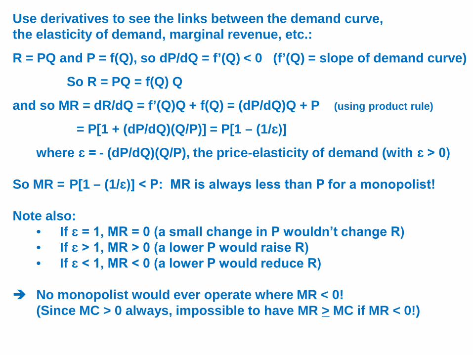
Use derivatives to see the links between the demand curve, the elasticity of demand, marginal revenue, etc.:

R = PQ and P = f(Q), so dP/dQ = f’(Q) < 0 (f’(Q) = slope of demand curve)

So R = PQ = f(Q) Q

and so MR = dR/dQ = f’(Q)Q + f(Q) = (dP/dQ)Q + P (using product rule)

= P[1 + (dP/dQ)(Q/P)] = P[1 – (1/ɛ)]

where ɛ = - (dP/dQ)(Q/P), the price-elasticity of demand (with ɛ > 0) So MR = P[1 – (1/ɛ)] < P: MR is always less than P for a monopolist! Note also:

• If ɛ = 1, MR = 0 (a small change in P wouldn’t change R) • If ɛ > 1, MR > 0 (a lower P would raise R) • If ɛ < 1, MR < 0 (a lower P would reduce R)

No monopolist would ever operate where MR < 0! (Since MC > 0 always, impossible to have MR > MC if MR < 0!)

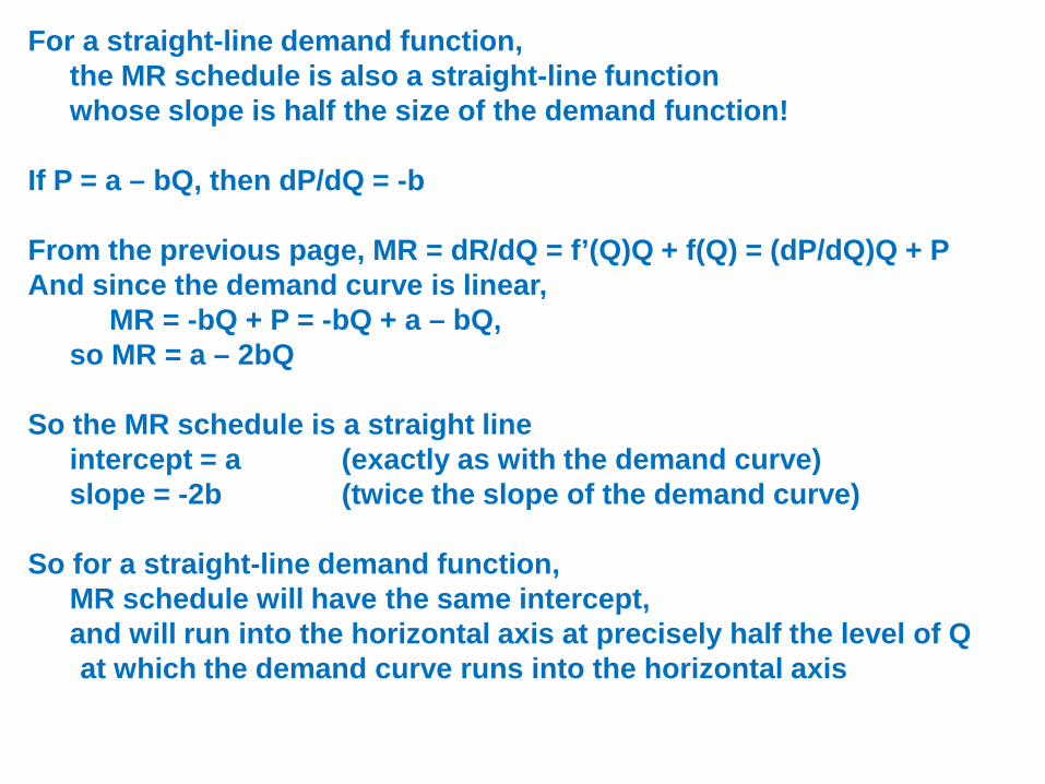
For a straight-line demand function, the MR schedule is also a straight-line function whose slope is half the size of the demand function! If P = a – bQ, then dP/dQ = -b From the previous page, MR = dR/dQ = f’(Q)Q + f(Q) = (dP/dQ)Q + P And since the demand curve is linear, MR = -bQ + P = -bQ + a – bQ, so MR = a – 2bQ So the MR schedule is a straight line intercept = a (exactly as with the demand curve) slope = -2b (twice the slope of the demand curve) So for a straight-line demand function, MR schedule will have the same intercept, and will run into the horizontal axis at precisely half the level of Q at which the demand curve runs into the horizontal axis

For a straight-line demand function: ɛ = -[ΔQ/Q]/[ΔP/P] = -[1/(ΔP/ΔQ)](P/Q) [ΔP/ΔQ)] = slope of D curve, and is constant P/Q falls as Q rises (and P falls) So ɛ falls in absolute value as Q rises

when MR is positive: ɛ > 1 R increases as P falls and Q rises

when MR is zero: ɛ = 1 R won’t change in response to small changes in P, Q thus, revenue is maximized (WARNING: this is NOT the same

as maximizing profit!)

when MR is negative: ɛ < 1 R decreases as P falls and Q rises

ɛ > 1 ɛ = 1

ɛ < 1

Profit-maximizing equilibrium of the monopolist: to find profit-maximizing output, we need to look ONLY at the MR and MC curves: as usual, produce more Q if MR > MC, less Q if MR < MC

• Q1 is too little output (MR > MC) – so increase Q • Q2 is too much output (MR < MC) – so reduce Q • profits are maximized at Q*

To determine monopolist’s costs, profits, etc.: first locate profit-maximizing level of output, Q* -- need only MR and MC to do this then determine the highest price P* the monopolist can charge in order to sell Q* -- need only the demand curve for this then determine ATC*, = ATC at Q* -- need only the ATC curve for this next, get the difference between P* and ATC*: profit per unit to get total profit, multiply profit per unit times # of units sold, i.e., find (P* - ATC*) ×Q*

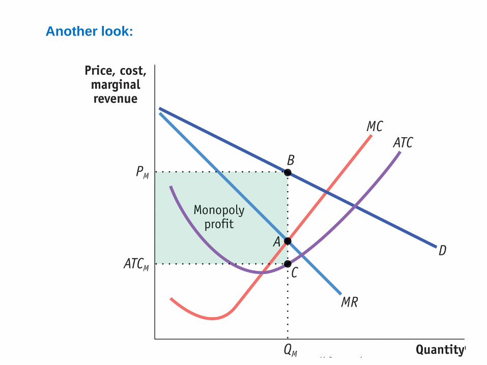
Figure 13.7 The Monopolist’s Profit Krugman and Wells: Microeconomics, Third Edition Copyright © 2013 by Worth Publishers

Another look:

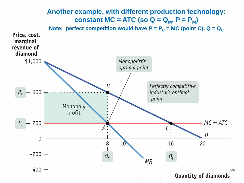
Figure 13.6 The Monopolist’s Profit-Maximizing Output and Price Krugman and Wells: Microeconomics, Third Edition Copyright © 2013 by Worth Publishers

Another example, with different production technology: constant MC = ATC (so Q = QM, P = PM)

Note: perfect competition would have P = PC = MC (point C), Q = QC

Figure 13.8 Monopoly Causes Inefficiency Krugman and Wells: Microeconomics, Third Edition Copyright © 2013 by Worth Publishers

Now consider the effect of monopoly vs. perfect competition on total/consumer/producer surplus: Perfect competition has P = MC, while monopoly has P > MR = MC. So monopolist always…

• charges P > MR = MC (since P > MC, “unfair price”) • restricts Q below the competitive level • thus, deadweight loss (see “DL” in Figure (b)) • earns positive (“excess”) economic profit – i.e.,

accounting profit that exceeds “normal” accounting profit

perfect competition

Exactly the same results with a different technology:

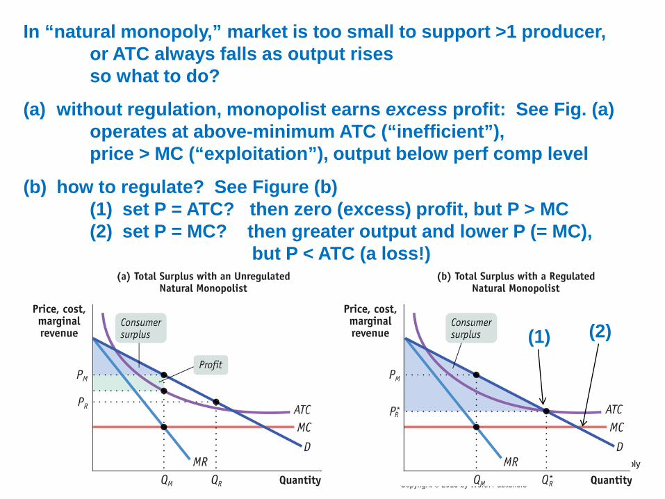
Figure 13.9 Unregulated and Regulated Natural Monopoly Krugman and Wells: Microeconomics, Third Edition Copyright © 2013 by Worth Publishers

In “natural monopoly,” market is too small to support >1 producer, or ATC always falls as output rises so what to do?

(a) without regulation, monopolist earns excess profit: See Fig. (a) operates at above-minimum ATC (“inefficient”), price > MC (“exploitation”), output below perf comp level

(b) how to regulate? See Figure (b) (1) set P = ATC? then zero (excess) profit, but P > MC (2) set P = MC? then greater output and lower P (= MC), but P < ATC (a loss!)

(1) (2)

Price discrimination

Monopolist can charge different consumers a different price for the exact same product – provided it can keep them separate

MC is the same for each type of consumer, so charge a price for each type that will equate MR and MC:

• Raise prices on customers with low price-elasticity of demand (reduces Q, raises R)

• Cut prices for customers with high price-elasticity of demand (raises Q, raises R)

examples: • senior/student ticket prices (movies, transportation) • vacation fares (planes, trains) • discount coupons (low vs. high-income) • doctors, dentists: sliding scales • university financial aid • quantity/volume discounts (case prices, 2nd item for 50% off…) • store brands vs. own brand

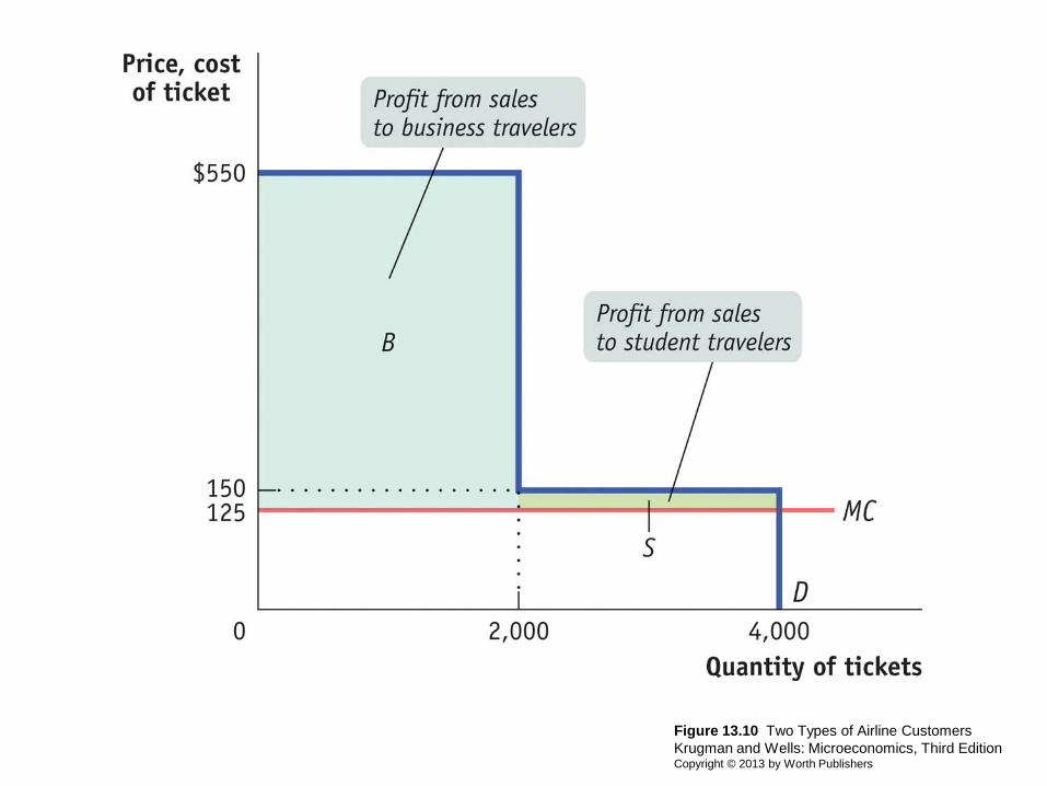
Figure 13.10 Two Types of Airline Customers Krugman and Wells: Microeconomics, Third Edition Copyright © 2013 by Worth Publishers

Figure 13.11 (a) Price Discrimination Krugman and Wells: Microeconomics, Third Edition Copyright © 2013 by Worth Publishers

Figure 13.11 (b) Price Discrimination Krugman and Wells: Microeconomics, Third Edition Copyright © 2013 by Worth Publishers

Figure 13.11 (c) Price Discrimination Krugman and Wells: Microeconomics, Third Edition Copyright © 2013 by Worth Publishers

Like the perfect competitor, the monopolist has a supply curve – but it’s not the same as the perfect competitor’s (= the MC curve) As demand curve shifts up, MR schedule shifts up too, and so equilibrium P-Q combination changes from a to b This runs roughly parallel to, but isn’t the same as, the MC curve

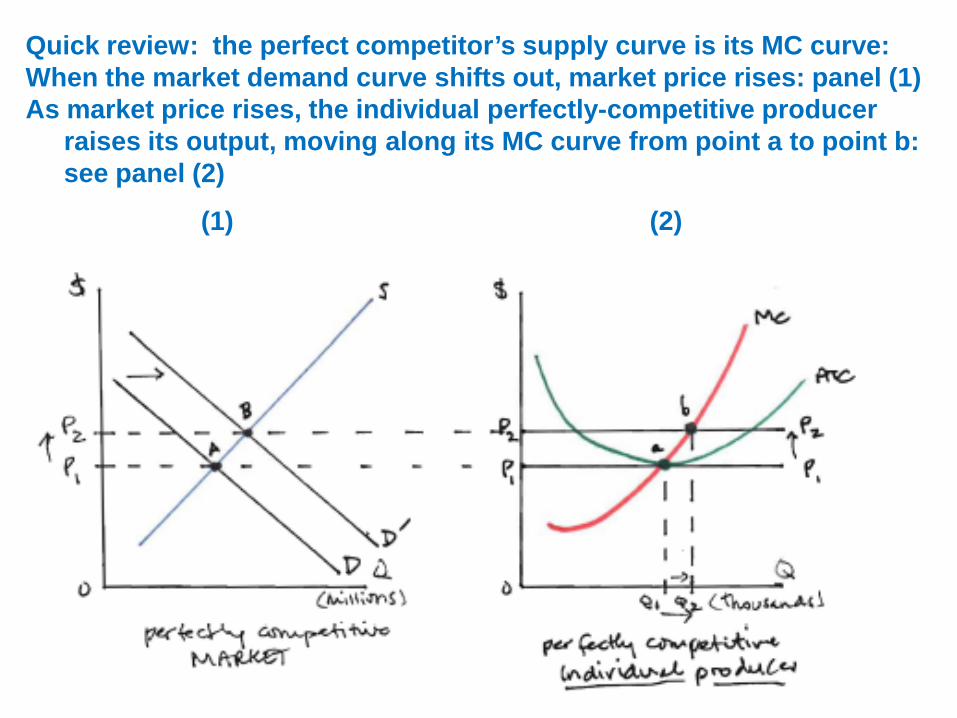
Quick review: the perfect competitor’s supply curve is its MC curve: When the market demand curve shifts out, market price rises: panel (1) As market price rises, the individual perfectly-competitive producer raises its output, moving along its MC curve from point a to point b: see panel (2)

(1) (2)