Payload Pointing from Mobile Robots

Deepak Bapna

CMU-RI-TR-98-08

Submitted in partial fulfillment of the

requirements for the degree of

Doctor of Philosophy

in the field of Robotics

The Robotics InstituteCarnegie Mellon University

Pittsburgh, PA 15213

February 20, 1998

Payload Tracking from Mobile Robots 3

Abstract

Payload tracking maintains alignment between a payload and a target while both payload and target may be moving. This research investigates the generic problem of tracking from a mobile robot. A tracking strategy based on subsystem interactions is developed along with tools to model and evaluate payload tracking, metrics for evaluating tracking configura-tions, and guidelines for developing configurations suitable for payload tracking from mobile robots. The strategy was implemented to design a communication system to achieve high bandwidth communication from a desert exploring mobile robot using active pointed high gain antennas.

Tracking is important for many applications including high bandwidth communication enabled by pointing of high gain antennas and active camera vision. In the case of moderate speeds across rough terrain, tracking demands high slew rates and large motion ranges due to vehicle motion disturbances. This differs from satellite antenna tracking or telescope pointing where the need is for very high precision but incurred motion rates are small. Moreover, mobile robots are commonly mass and power limited. Attaining tracking stabil-ity requirements coupled with large articulation ranges, high slew rates, as well as low mass and power makes the problem of payload tracking from mobile robots challenging.

This research considers the complete robot (mechanism, planning and control) to achieve precision tracking. This is important because an independent fine pointing device such as a gimbal alone- without cooperation from locomotion, suspension and isolation devices - might not provide the angular excursions and disturbance rejection needed in rough terrain. As the terrain roughness and corresponding excursions and disturbances increase, so does the need for robot subsystems to functionally cooperate to achieve payload tracking.

Payload Tracking from Mobile Robots 4

A Payload Tracking Strategy for Mobile Robots v

List of Figures ...................................................................................... ix

List of Tables ...................................................................................... xi

Acknowledgments ..................................................................................... 13

CHAPTER 1 Introduction ............................................................. 15

Motivation ................................................................................................... 18

Problem Description .................................................................................... 19Problem Statement ................................................................................................19Problem Scope ......................................................................................................20Application Area ...................................................................................................21Robot Design Elements That Impact Tracking .....................................................22

Methodology ................................................................................................ 23Modeling ...............................................................................................................24Synthesis ...............................................................................................................24Analysis ................................................................................................................25

Contents

Contents

A Payload Tracking Strategy for Mobile Robots vi

Simulation .............................................................................................................25Building, Testing, and Demonstration ..................................................................25

CHAPTER 2 Background ............................................................. 27

Mechanism ..................................................................................................28Locomotion ...........................................................................................................28Suspension ............................................................................................................30Pointing Device ....................................................................................................31

Control .........................................................................................................33Related Control Background ................................................................................34

Planner .........................................................................................................34Related Planning Background ..............................................................................34

CHAPTER 3 Methodology ............................................................ 37

Design Process .............................................................................................39

Task Specification ........................................................................................39

Component Screening ..................................................................................42Locomotion Evaluation - Vehicle Smoothing Factor ............................................43Pointing Device Evaluation - Coupling Indices ...................................................48Sensor Evaluation - Sensor Criticality Factor .....................................................60Dependence on Planner .......................................................................................62

Design Synthesis and Evaluation ................................................................66

Design Selection ..........................................................................................69

Dynamic Simulation ....................................................................................70

CHAPTER 4 Case Study- Communication from a Mobile Robot . 71

Atacama Desert Trek ...................................................................................71

Task Specifications ......................................................................................72

Screening Component Configurations .........................................................74Locomotion ...........................................................................................................74Antenna Pointing Device ......................................................................................76Payload .................................................................................................................76Sensor ...................................................................................................................77Planner .................................................................................................................83

A Payload Tracking Strategy for Mobile Robots vii

Contents

Tracking Design- Synthesis and Evaluation ................................................ 83

Design Selection .......................................................................................... 87

Dynamic Simulation .................................................................................... 88

Detailed Design ........................................................................................... 88Locomotion ...........................................................................................................90Antenna Pointing Mechanism ..............................................................................90State Sensors .........................................................................................................94Controller for Pointing Mechanism .....................................................................95

CHAPTER 5 Experiments ............................................................. 97

Long Range Communication ....................................................................... 98

Performance Quantification ......................................................................... 99Experimental Setup ...............................................................................................99Data Logged .......................................................................................................100Derivation of the Performance Parameters .......................................................102Dependence on Various Parameters ..................................................................104

Communication Link Performance ........................................................... 112

Pointing Error Observability Limitation ................................................... 115

Experimental Conclusions ......................................................................... 116

CHAPTER 6 Summary and Conclusions .....................................117

Contributions ............................................................................................. 118

Lessons Learned ........................................................................................ 121

Research Directions ................................................................................... 121

APPENDIX A Dynamic Model ........................................................ 123

APPENDIX B References ................................................................ 127

Contents

A Payload Tracking Strategy for Mobile Robots viii

A Payload Tracking Strategy for Mobile Robots ix

FIGURE 1-1 Payload Tracking .................................................................................................... 15

FIGURE 1-2 Entire Robot Constitutes a Tracking System ......................................................... 16

FIGURE 1-3 Elements of Tracking ............................................................................................. 17

FIGURE 1-1 Communication from Mobile Robots .................................................................... 21

FIGURE 1-2 Methodology .......................................................................................................... 23

FIGURE 2-1 Articulated Vehicle Concepts ................................................................................. 29

FIGURE 2-2 Suspension (a) Passive (b) Active .......................................................................... 31

FIGURE 2-3 RANGER: (a) State Space Vehicle Model (b) Hazard Detection and Avoidance . 35

FIGURE 3-1 Design Process ....................................................................................................... 40

FIGURE 3-2 VSF Versus Coupling ............................................................................................. 42

FIGURE 3-3 (a) Conventional 4-wheel (b) Pitch Articulation (c) Rocker-Bogie configuration 43

FIGURE 3-4 Dependence on Locomotion Topology .................................................................. 45

FIGURE 3-5 Terrain for Simulation ............................................................................................ 46

FIGURE 3-6 The Cart and Pendulum System- (a) ...................................................................... 48

FIGURE 3-7 The Cart and Pendulum System- (b) ...................................................................... 51

FIGURE 3-8 Pointing Devices - a) Azimuth/Elevation Topology b) X/Y Topology .................. 56

FIGURE 3-9 Kinematic Coupling - (a) Az/El Pointing (b) X/Y Pointing ................................... 56

FIGURE 3-10 Dynamic Coupling Factor - a) Az/El Topology b) X/Y Topology ......................... 57

List of Figures

List of Figures

A Payload Tracking Strategy for Mobile Robots x

FIGURE 3-11 Dependence on Pointing Topology ........................................................................58

FIGURE 3-12 Kinematic Coupling for Overhead Target - (a) Az/El Pointing (b) X/Y Pointing .59

FIGURE 3-13 Dependence on Vehicle Speed ................................................................................64

FIGURE 3-14 Dependence on Obstacle Size ................................................................................65

FIGURE 3-15 Dependence on Obstacle Distribution ....................................................................67

FIGURE 3-16 Design Generation and Evaluation .........................................................................69

FIGURE 4-1 Communication Using Omnidirectional Antennas ................................................72

FIGURE 4-2 VSF for a Pitch Articulated and a Rocker-Bogie Chassis ......................................75

FIGURE 4-3 Parameters for Kinematic Coupling .......................................................................77

FIGURE 4-4 Kinematic Coupling ................................................................................................78

FIGURE 4-5 Reference Frames ...................................................................................................79

FIGURE 4-6 Terrain .....................................................................................................................85

FIGURE 4-7 PID Control- Pointing Offset Vs. Time ..................................................................89

FIGURE 4-8 Nomad’s Pitch Articulated Chassis ........................................................................90

FIGURE 4-9 Transforming Chassis (a) Compact (b) Deployed ................................................91

FIGURE 4-10 Pointing Specifications- a) Pointing Angular Range b) Pointing Angular Rates ...91

FIGURE 4-11 Antenna Pointing Mechanism ................................................................................93

FIGURE 4-12 Block Diagram for Pointing ...................................................................................95

FIGURE 5-1 Long Range Communication Experiment ..............................................................98

FIGURE 5-2 Experimental Setup ................................................................................................99

FIGURE 5-3 GPS Plot ...............................................................................................................100

FIGURE 5-4 Commanded Current vs. Monitored Current ........................................................103

FIGURE 5-5 Pointing Performance vs. Speed (level terrain) ....................................................106

FIGURE 5-6 Pointing Performance vs. Turning Radius ............................................................107

FIGURE 5-7 Experiments to Evaluate Dependence on Obstacle Size ......................................108

FIGURE 5-8 Pointing Performance vs. Obstacle Size ...............................................................110

FIGURE 5-9 Optimal Trajectory Planning ................................................................................ 111

FIGURE 5-10 Nomad Chassis (a) Compact (b) Deployed ........................................................ 111

FIGURE 5-11 Path for Testing Dependence on Wheel Base .......................................................112

FIGURE 5-12 Pointing Performance Vs. Wheel Base ................................................................113

FIGURE 5-13 Communication Overview ....................................................................................114

FIGURE 5-14 Data Rate ..............................................................................................................114

FIGURE 5-15 Antenna Offset vs. Data Rate ...............................................................................115

FIGURE A-1 Simplified Model for Simulation ..........................................................................123

A Payload Tracking Strategy for Mobile Robots xi

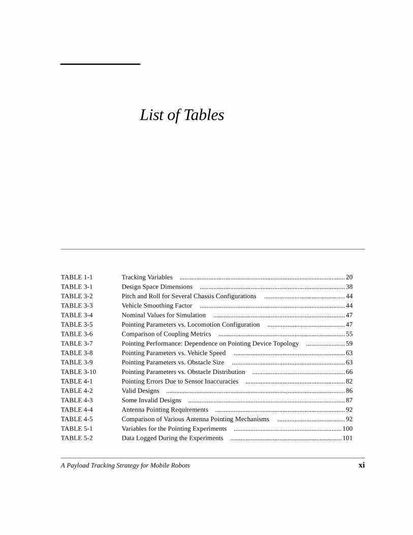
TABLE 1-1 Tracking Variables .................................................................................................. 20

TABLE 3-1 Design Space Dimensions ...................................................................................... 38

TABLE 3-2 Pitch and Roll for Several Chassis Configurations ................................................ 44

TABLE 3-3 Vehicle Smoothing Factor ...................................................................................... 44

TABLE 3-4 Nominal Values for Simulation .............................................................................. 47

TABLE 3-5 Pointing Parameters vs. Locomotion Configuration .............................................. 47

TABLE 3-6 Comparison of Coupling Metrics ........................................................................... 55

TABLE 3-7 Pointing Performance: Dependence on Pointing Device Topology ....................... 59

TABLE 3-8 Pointing Parameters vs. Vehicle Speed .................................................................. 63

TABLE 3-9 Pointing Parameters vs. Obstacle Size ................................................................... 63

TABLE 3-10 Pointing Parameters vs. Obstacle Distribution ....................................................... 66

TABLE 4-1 Pointing Errors Due to Sensor Inaccuracies ........................................................... 82

TABLE 4-2 Valid Designs .......................................................................................................... 86

TABLE 4-3 Some Invalid Designs ............................................................................................. 87

TABLE 4-4 Antenna Pointing Requirements ............................................................................. 92

TABLE 4-5 Comparison of Various Antenna Pointing Mechanisms ........................................ 92

TABLE 5-1 Variables for the Pointing Experiments ................................................................ 100

TABLE 5-2 Data Logged During the Experiments .................................................................. 101

List of Tables

List of Tables

A Payload Tracking Strategy for Mobile Robots xii

TABLE 5-3 Dependence on Vehicle Speed ..............................................................................105

TABLE 5-4 Dependence on Turning Radius ...........................................................................106

TABLE 5-5 Dependence on Obstacle Height ..........................................................................109

TABLE 5-6 Dependence on Wheel Base ................................................................................. 112

Acknowledgements 13

Acknowledgments

First and foremost, thanks to my wife, Shivali. Even though I was constantly busy since our wedding (first with the Nomad project and then with my thesis), Shivali never complained. Shivali, you will probably never know how much your love and support means. How lucky I am to have you as my life partner, friend, and motivator.

To my parents and sisters, thank you for everything. This thesis is dedicated to you, to your love, and to everything you do for all of us in the family. To my uncle, aunt, cousins, Dimple and Priyank, brother-in-law, Mohit, and niece Mumal, thank you for being part of my extended family and ensuring that I did not have to worry about anything.

This is also dedicated to Anik, born a month before my defense, who changed the world for us and made it much more beautiful and enjoyable. To my mother-in-law, who was here during Anik’s birth and later, making sure I worked on my thesis and did not get distracted, thank you for all your help.

Finally, thank you to my advisors John Bares and Red Whittaker, for your guidance and encouragement. Red gave me the opportunity to work on this exciting project and had con-fidence in me. Thank you both for your thoughtfulness and being great advisors. I learnt a lot from both of you and will always be grateful.

I express my sincere appreciation to Mike Luniewicz, Eric Krotkov, and Yangsheng Xu for serving on my thesis committee. And to Dot, who helped in numerous ways by teaching how to face Red, be confident, be comfortable in FRC environment, and much more.

Payload Tracking from Mobile Robots 14

Thanks to all my friends for their constant support. I appreciate the help of the members of the Atacama Desert Trek Team, especially, Eric Rollins, Nick Vallidis, Mark Sibenac, Jim Teza, Ben Shamah, Mark Mai-mone, Hans Thomas, Paul Parker, Jack Silberman, Stewart Moorehead, Michael Parris, Alex Foessel, Steven Dow, Dimitrios Apostolopoulos, and Lalitesh Katragadda. The design, integration and testing of the antenna pointing mechanism would not have been possible without your help. I will miss working with you. Thank you Murli and Sundar for all the useful discussions and the last minute preparations. And special thanks to Vipul, Saurabh, Tarun, Murli, Sundar, and Anil, who were always there when I needed them.

Finally, thank you to all the people at The Robotics Institute who made the last four and half years at this place so wonderful through your friendship and support. I am going to miss my colleagues at the Robotics Institute a lot.

Introduction 15

CHAPTER 1 Introduction

Payload tracking maintains alignment between a payload and a target while both pay-load and target may be moving. The ability to achieve payload tracking while roving is important for mobile robots as it can enable a wide variety of tasks including tele-operation, wireless communication, mobile surveying and reconnaissance, coopera-tive manipulation and active vision. Mobile robot payload tracking requires high slew

TargetTarget Trajectory

Payload

Mobile Robot

time t1 time t2

time t3time t1 time t2

time t3

FIGURE 1-1: Payload Tracking

16

rates and large articulation ranges in order to stabilize and orient a payload while moving over uneven ter-rain. Both requirements become more demanding as speed and terrain roughness increase. Traditional approaches from other domains typically append a pan/tilt (or gimbal) to the moving vehicle or platform. Although precision can be on the order of micro-radians, these pointing mechanisms are massive and require high power. For instance, during rough seas, antenna dishes on deep sea drilling platforms are stabilized and aimed with massive high power positioners. Likewise, a gun barrel aiming system on an M-1 tank tracks tar-gets while the battle tank is moving at high speed but must be quite massive. Mobile robots (and especially exploratory robots), however, are usually limited in mass, power and available space, necessitating precision tracking approaches that can meet these additional requirements.

This research considers the complete robot system to achieve precision tracking (Figure 1-2). That is, mech-anism, planning and control at different levels - traction elements (wheel, legs or hybrid), chassis, suspen-sion and pointing mechanisms- combine to achieve precision payload tracking objectives. This is important because an independent pointing device (e.g, gimbal), without cooperation from locomotion (wheels/legs, chassis, suspension) and planner, may not be able to provide the large torques, angular excursions, and dis-turbance rejection needed in rough terrain. As terrain roughness and vehicle excursions and disturbances increase, so do the challenges to achieving payload tracking.

When considering the entire mobile robot as a payload tracking system, the principal elements affecting tracking performance are mechanism, control and the local path planner (see Figure 1-3).

Mechanism: In this research, the term “mechanism” denotes locomotion and pointing devices:

Payload

Body

Suspension

Vehicle/TerrainInteraction

Chassis

Pointing

FIGURE 1-2: Entire Robot Constitutes a Tracking System

Planning

Which Path? ? ? ? ?

Top View

Target Trajectory

Introduction 17

• Locomotion is comprised of a robot’s traction elements (wheel/leg), suspension and chassis. Suspension (if present) can be active or passive and isolates high frequency terrain disturbances from payloads. Tracking performance may differ with alternate locomotion modes (wheeled/legged/hybrid) and traction element char-acteristics.

• A Pointing Device removes disturbances not suppressed by locomotion, suspension and isolation devices as well as aims the payload at the target. It may be mechanical (e.g., a precision gimbal) or electronic (e.g., phased array in some cases). It might consist of several stages. For example, pointing might consist of an iso-lation stage that isolates payload(s) from motion disturbances. Methods of isolation include passive gimbal suspension, gyroscopic stabilization, magnetic bearings and inertial platforms.

Control & Sensing: The control of all elements of locomotion and pointing devices contribute to tracking per-formance. Steering mode (Ackerman vs. skid-steering) as well as individual wheel control (e.g., position con-trol vs. velocity control vs. torque control) can effect tracking performance. In general, controllable suspensions (active or semi-active suspension) have far better terrain smoothing capabilities than passive suspensions and can greatly enhance tracking performance. Pointing device control is the most critical factor in tracking. Controller performance is often limited by state sensors, so appropriate sensor configuration (accuracy, update rate, etc.) is important.

Path Planner: The path planner can contribute to achieving tracking objectives in several ways. For example, it can avoid paths that may be difficult from a tracking perspective (e.g., paths that may induce large excursions of the body or induce high rate disturbances) or it can provide data for feedforward control (such as warning about upcoming boulders and craters).

TRACKING

Control & Sensing

Locomotion

Path Planner

FIGURE 1-3: Elements of Tracking

Pointing

Mechanism

- Wheel /Legs- Chassis- Suspension

18

1.1 Motivation

Communication at extended ranges is an important capability for outdoor mobile robots. Achieving high data rate communication over such an extended range (> 2-3 km) poses challenging problems. Current mobile communication systems use low gain, omnidirectional antennas in order to ensure coverage while travelling. However, a fundamental problem with this approach is that the data rate of such a link is limited. The data rate can be increased by boosting power, which is effective for large ground vehicles such as battle tanks. However, the resulting escalations in power budget and component size are not feasible for small rov-ing vehicles. Alternately, directional antennas can be used to boost the data rate without increasing power requirements. In this case the link’s performance depends on the pointing accuracy of the directional antenna. The challenge is to keep the antenna pointed towards the receiver while the robot is moving. In some cases such as a mobile robot-orbiting satellite (non geo-synchronous) link, the receiver may also be moving.

Communication over long distances is also important for robotic exploration of other planets. Future mis-sions will have ambitious goals in terms of exploration, information transmission and reduced cost. For example, a 1000 km lunar traverse was proposed, where a rover would be used to visit historic sites and involve audience participation through teleoperation and high-quality video images [69]. Such a mission would require high data rate transmission from the robot to Earth at relatively low power levels (as total power is limited). This would be possible only if the angular offset between transmitter and receiver anten-nas is small. A precision tracking ability can therefore enable the bandwidth required for such long distance robotic exploration by maintaining a precise line-of-sight lock between the transmitting antenna on a lunar robot and the receiving antenna on Earth.

Another potential problem is that tracking difficulty may increase on planets. [44] performed a dynamic analysis of wheeled planetary rovers and observed that excursions were much higher under low gravity con-ditions. Exploiting the entire robot to achieve tracking performance may be necessary in this case, not only because chassis excursions are dependent on gravity, but also because severe limits exist on mass and power.

Payload tracking also pertains to active control and stabilization of sensors. Active control of sensors and cameras is important for autonomous navigation as it can reduce perceptual throughput by pointing the sen-sor to an exact location of interest [37]. Stabilization of sensors and payloads is important for many robotic applications. For instance, an autonomous construction machine may need a stabilized laser scanner in order to achieve consistent imagery. For certain applications, payloads like cameras and scientific instruments may also need stabilization. The issue of stabilization can be considered to be a subset of the tracking prob-lem, where the target is stationary in an inertial frame.

Payload tracking may be useful for enabling optical communication from mobile platforms. Optical (or laser) communication enables high bandwidth transmission at low power levels using a coherent light beam. However, line-of-sight pointing accuracy requirements are severe (of the order of micro-radians) and pose a major challenge, especially for communication from a mobile platform. A systemic strategy, as developed in this research, can prove useful in achieving mobile optical communication.

Introduction 19

Consider a positioner that is mounted to and controlled independently of the mobile robot base to achieve desired payload tracking requirements. Rather than using the positioner as a tracking system, using the entire robot sys-tem for tracking has certain advantages, including:

• Mass and power savings: Disturbance torques to the pointing mechanisms can be lowered by appropriate locomotion and planner configuration, thus yielding substantial mass and power savings in mechanism design.

• Systemic simplicity: An appropriate locomotion and/or isolation mechanism can drastically reduce pointing needs. In certain cases it might be possible to satisfy subsequent pointing needs by incorporating off-the-shelf gimbals and positioners.

• Easier payload adaptation: Developing a specialized tracking technique for each individual application/pay-load may not be necessary. A robot may act as a tracking platform capable of adaptation to diverse payload dimensions, masses and tracking requirements.

Examples will illustrate these points in the following chapters.

1.2 Problem Description

1.2.1 Problem Statement

Mobile robot tracking demands large articulation ranges and high slew rate capability. Moreover, mobile robots are commonly limited in mass and power. This makes tracking systems for satellites and telescopes, which typi-cally have reduced slew rate requirements, inappropriate for mobile robot applications. Likewise target tracking systems on tank guns, though similar in functionality, are not suitable for mobile robots due to their large mass.

Payload tracking is addressed in other domains, but the solutions from those domains are not directly applicable to the mobile robot payload tracking problem either because power and mass constraints are less stringent (such as for battle tanks and oil rigs), or because slew rate requirements are less severe (such as for satellites and bal-loons). Tracking techniques are needed that 1) can achieve high stability while meeting articulation range, slew rates and target tracking requirements; and 2) have reasonably low mass and power. The concept of this work is to exploit the entire robot system to achieve the payload tracking objective instead of simply appending a “track-ing” device onto a mobile robot base. This leads to the following thesis statement:

“Develop tracking technique for mobile robot applications, by considering the entire robot as a tracking system (mechanism, planning and control) that satisfies stability requirements along with large articulation range, high

20

slew rates, low mass and power, and demonstrate the technique by achieving high bandwidth communica-tion from a mobile robot.”

High data rate communication over extended ranges is an important capability for mobile robots and is cho-sen as the application area for the thesis. This problem encompasses key tracking challenges from mobile platforms.

1.2.2 Problem Scope

Pointing performance depends on several parameters of locomotion, pointing mechanism, controller, state sensors and planner. Although the parameters vary across configurations, some of the common parameters are tabulated below (Table 1-1):

Description of a tracking problem includes the above variables and more, resulting in a large number of pos-sible options to be evaluated. The following limitations bound the scope of this research:

• Inertially stable target: This covers applications such as communications with a stationary receiver sta-tion (e.g., a geosynchronous satellite) or hilltop repeater as well as sensor stabilization applications.

• Wheeled locomotion: A large class of outdoor mobile robots are wheeled robots. Low power planetary explorers are also likely to be wheeled. Though less prevalent, legged machines can provide a more sta-ble platform than wheeled machines, and hence simplify the pointing problem. However, the scope of this thesis is limited to terrains more suited to wheeled locomotion.

• Rough, but not severe terrain: Only terrain traversable by wheeled machines (e.g., natural terrain,

, ~ 0.5D obstacles, where D is the wheel diameter) is considered.

TABLE 1-1: Tracking Variables

Item Variables

Robot Locomotion,

Suspension

Kinematics, wheel diameter, wheel width, wheel stiffness, wheel base, vehicle stance, suspension stiffness and damping, suspension kinemat-ics

Payload Inertia, mass

Pointing Mechanism Kinematics, inertias, mass, friction, damping

Pointing Controller Type, gains

State Sensors Accuracy, bandwidth, latency, noise spectrum

Planner Speed, path

Mission Terrain Soil characteristics, obstacle distribution and dimensions, underlying slopes

Target Trajectory

slopes 30≤ °

Introduction 21

• Moderate speed ( m/sec): This is a nominal speed for autonomous or teleoperated rovers over rough ter-rain.

• Angular tracking: Full tracking involves positioning the payload in all six degrees of freedom - three linear and three angular (x, y, z and rotation around each of these). Here, only angular motions are considered. This assumption of angular tracking is reasonable when the target is distant from the payload.

• Three locomotion configurations: This research examines three locomotion configurations in order to high-light the strategy. Once the methodology is illustrated on these configurations, it can be extended to other configurations using the procedure developed in the thesis.

• High angular speed, low precision tracking applications (angular rates on the order of /sec, precision on the order of mrad) like antenna pointing and camera pointing from mobile robots.

• Rigid mast: The mast (if present) on which the pointing mechanism is located is assumed to be rigid. The rigidity can be ensured in most of the cases by proper design.

• Application area: Communication from outdoor mobile robots fits well in the scope and is chosen as the application area.

1.2.3 Application Area

Active pointing of an antenna from a moving robot is chosen as the application area for this thesis. Further dis-cussions on pointing will be related to this area. High bandwidth distant range communication is an important problem for mobile robot applications. Using omnidirectional antennas, a range on the order of 1-2 km can nor-mally be achieved. This range is insufficient for many outdoor mobile tasks. One way to increase the range is to use an actively pointed high gain antenna (Figure 1-1).

Another way to increase the data rate and range is to increase the RF output power. Although this might be prac-tical in some cases, it is not for mobile robot applications where the power is limited. The typical efficiencies of the RF amplifiers are on the order of 10%; hence to increase output power by 1 W, 10 W input is required. Also the link margin is proportional to the square of the size of the dish, directly proportional to the output power, and

1≤

40°

FIGURE 1-1: Communication from Mobile Robots

Robot

Relay Station

Wireless

Communication

~ 10 km

22

inversely proportional to the square of the communication range. So to double the communication range, output power has to be quadrupled and the input power has to be increased by a factor of 40. This might work if the initial power is of the order of milli-watts. Also in certain cases, due to FCC limitations, radios are restricted in power. Thus, boosting the RF output power is not always practical. The approach used in this thesis is to use a higher gain antenna.

The particular task chosen for implementation of this strategy was high bandwidth communication for the Atacama Desert Trek. In addition to advancing robotic technologies for planetary exploration, involving the public was another key objective of this demonstration. The principal tool for enabling public participation was a high resolution panospheric camera [51]. In order to transmit its imagery (generated at 4-6 Hz) from the rover to a local control station and then to remote mission control sites, a high bandwidth (2 Mbps) reli-able communication link was paramount. As discussed earlier, this can be achieved using active pointing of high gain antennas.

1.2.4 Robot Design Elements That Impact Tracking

Various robot components including locomotion elements and pointing mechanisms can be combined to achieve precision tracking objectives. The control and planning which determine robot motion, in addition to the design of each mechanical component, influence tracking performance. The principal design elements that influence precision payload tracking from mobile robots can be lumped into mechanism, control (including sensing) and planning.

Mechanism: The requirements of large articulation and slew rates required for unstructured terrain cannot be achieved using traditional techniques while also meeting the low mass and power constraints of a mobile robot. Locomotion elements (wheels, chassis, suspension) and pointing mechanism design may need to be optimized together to meet the overall objectives. Also, an appropriate design can vastly simplify control needs. For example, simple gimballed pointing systems are subject to dynamic interaction problems and, when the payload center of gravity does not coincide with gimbal axes, large disturbances complicate con-trol. However, it may not always be possible to center-mount the payload; thus, the offset must be compen-sated in some other way. Other important issues are reliability, payload adaptation and coupling between various axes.

Control and Sensing: The control of locomotion (wheel/leg motion), suspension and pointing mechanism all affect pointing performance. For instance, a skid steer machine might have different pointing require-ments than a machine with Ackerman steering. Actively controlled suspensions can be used to accommo-date rough terrain while maintaining a level body. This might simplify the control needs for a pointing device but only at the expense of increased mass. Although active suspension might be an important way to approach the pointing problem, it is another considerable research problem in itself; as a result, it is not con-sider further here.

Introduction 23

In the design of control systems for pointing, mechanism performance requirements that must be considered include rejection of base motion disturbances and noise, tracking accuracy and dynamic response, and system stability and robustness. Some of these requirements contradict each other.

Sensing (of the vehicle as well as pointing state) is an important issue. Controller performance can only be as good as sensor accuracy. For pointing from mobile robots, high precision and accurate sensing at a high update rate is required to compensate for high disturbance rates. This is often the most challenging issue.

Planning: Path planning can be combined with predictive control to achieve better tracking performance. For instance, the planner can warn the pointing system of upcoming bumps and ditches. One way the planner can directly assist pointing is by determining appropriate driving speed and turning radius. The challenge here is to come up with parameters (speed, obstacle heights, turning radius) that will satisfy locomotion as well as pointing objectives.

1.3 Methodology

The methodology for developing payload tracking solutions for mobile robots is to synthesize, analyze and eval-uate a holistic model of tracking (including mechanism, sensors, planning, control and terrain) followed by building, testing and demonstration.

SYNTHESIS

ANALYSIS

TESTING

MODELLING

- Terrain- Wheel- Chassis- Suspension- Isolation- Pointing Devices- Control

DEMONSTRATION- Performance Metrics

- Components Configurations- Tracking Topology- Tracking Designs

- Detail dynamic simulation (including controller)

Design Process

BUILDING

SIMULATION

- Path Planning- Communication

FIGURE 1-2: Methodology

24

A tracking topology, for this research, consists of a specific locomotion configuration, pointing device con-figuration, sensor set, and motion planner. Appreciable literature exists on each of these components (loco-motion, pointing devices, state sensors, planner) and an initial set of acceptable component configurations are obtained by analyzing these with respect to tracking needs. These components are then combined to obtain tracking topologies. Tracking “designs” are then synthesized by assigning parameter values to each of the topologies.

Analysis and simulation enables performance estimates to be generated before actually building the system. Mathematical models are necessary both for system analysis and performance simulation. The cycle of syn-thesis, analysis and evaluation is repeated until an acceptable design is reached. After achieving confidence in a given design, building, testing and experimentation follow. Demonstration is the final step.

Each of above steps are discussed in detail in the following subsections.

1.3.1 Modeling

A mathematical model of the system is essential for analysis and evaluation. The mathematical models used/developed in the thesis include:

• Terrain: The terrain is modeled as a sinusoid. Diverse terrain can be generated by combining sinusoids of various amplitudes and phases. Traversing steps (especially in low gravity) is the worst-case tracking scenario and is used for generating requirements.

• Chassis: For the purpose of tracking, the most important functionality is to provide smooth motion. The body orientation (roll and pitch) is expressed as a function of wheel position using a set of algebraic equations.

• Pointing Device: Pointing devices are modeled as serially connected linkages. In this case, they can be treated as simple manipulator arms and can be analyzed using well developed methods for analysis of manipulators.

• Sensors: Sensors are specified by their accuracy, bandwidth and noise.

• Communication: The communication is modeled using well-known equations for link analysis.

1.3.2 Synthesis

Synthesis generates tracking designs by a three-step sub-process:

1. Screening from a collection of all possible robot design elements (locomotion configuration, pointing configuration, sensor set, and planner) a set of those components, that when assessed at the component level, meet some minimal criteria for application in a payload-tracking robot design. Several metrics, as discussed in Chapter 3, are developed for screening the initial set of components.

2. Combining various components from the screened set generated in the previous step into tracking topol-ogies

Introduction 25

3. Assigning an initial set of numeric values to the design parameters of the topology. This step results in a “design”.

1.3.3 Analysis

Analysis, through kinematic simulations and analytic techniques, predicts approximate performance of the designs generated by the synthesis process. From the designs that eventually meet requirements some are selected for evaluation in the next step. Selection at this level may be based on the relative weighting of various system objectives for the particular application, e.g. in one application, it may be that minimal power is of great-est importance while in another, it may be minimal mass.

1.3.4 Simulation

Evaluation then applies dynamic simulation to designs selected from the analysis output. Dynamic simulation produces higher fidelity performance predictions of the designs but is more expensive than the kinematic simula-tion applied during the evaluation process. Finally, designs may be tuned during the evaluation process to further optimize performance.

1.3.5 Building, Testing, and Demonstration

The next step after simulation is building the pointing mechanism. The pointing mechanism is built based on the simulation results. Mechanism, sensor, controller and planner are integrated and tested at various stages of devel-opment. Finally, the system is demonstrated to achieve high bandwidth communication at distant ranges. This is described in detail in Chapters 4 and 5.

The next chapter presents the summary of background research on topics related to tracking from mobile robots.

26

Background 27

CHAPTER 2 Background

Tracking performance of mobile robots depends upon locomotion, planning, pointing devices and controls. Although few devices exist that are capable of tracking from moving robots traversing natural terrain, extensive research has been done in tracking for other applications. While several issues are unique to tracking from mobile robots, there is some commonality with other applications.

Research for tracking from mobile robots primarily emphasizes the perception and control aspects of tracking, especially vision-based tracking. The majority of prior work is associated with manipulators or mobile robots in structured environments where the target has slow motion relative to the payload. Issues of mass and power constraints are not addressed. [1] presents a mathematical theory of visual tracking of a rigid 3-D target of known shape moving in 3-D. It attempts to develop correspon-dence free tracking and eliminate the limitations inherent in the optical flow formal-ism. [19] proposes a controller that combines self-tuning prediction and control (STPC) to manipulator arm trajectory tracking. The controller has two feedback loops: One is used to minimize prediction error; the other is designed to track the set point input. [72] describes a real-time vision service that recognizes and monitors non-rigid moving objects in natural scenes. The tracking routine uses correlation-based optical flow for both recognizing and monitoring the camera-relative motion of the moving objects. [37] addresses the usefulness of actively controlled pointable sen-sor heads for off-road mobile robot navigation. The research addresses the physical motion of a sensor head and indicates that maneuverability is limited by mass and power.

28 Background

The main challenge in achieving precision payload tracking from mobile robots is to compensate for the large, fast chassis motions that occur in rough terrain. Also, the mass, size and power constraints for mobile robots introduce much subsystem dependence. As a result, the systemic approach can provide improved tracking performance. The entire robot (mechanism, planning and control) can be thought of as a precision tracking system where locomotion elements (wheel/leg), suspension, path planner and fine pointing devices combine and functionally cooperate to achieve precision tracking objectives.

The approach undertaken here for payload tracking from mobile robots incorporates locomotion configura-tion, suspension, fine pointing devices and path planning. The design elements can be classified into mecha-nism, control and planning and are discussed below along with the existing work.

2.1 Mechanism

The role of locomotion for tracking is to isolate payloads, to the extent possible, from terrain roughness. The pointing device actively orients the payload: it must provide angular excursion and speeds to satisfy the tracking requirements. Therefore, the requirements on the fine pointing devices are relaxed as the isolation abilities of chassis and suspension, increase. Primary requirements applicable to the mechanism are:

• High slew rates and large articulation angles: Vehicle motion disturbances impose large torque requirements which lead to large/heavy actuators. Any strategy that compensates for vehicle distur-bances, thus reducing slew rates and corresponding torques, may be useful. The goal is to design a loco-motion mechanism that minimizes disturbance to the pointing mechanism while satisfying the locomotion objectives.

• Mass/Power limit: Mobile robots are constrained to low mass and power, which contradicts the require-ments of large articulation and high slew rates. Therefore, it is necessary to develop systemic design and control strategies that can allow large excursion and slew rates with reasonable mass and power.

• Payload adaptation: Different payloads may have different sizes, shapes, mass, moments of inertia and tracking requirements. Therefore, it is desirable that the payload tracking technique be parametric and thus capable of handling diverse payloads. The issue is not how to design a specific control system, but how to develop a strategy that can accommodate a variety of tracking tasks.

In addition to these requirements, others specifically related to the locomotion, suspension, isolation and fine pointing device are discussed below.

2.1.1 Locomotion

Locomotion configuration is a key parameter in mobile robot payload tracking. An ideal locomotion config-uration for tracking purposes would be able to directly stabilize a payload without the need for payload iso-lation. The main issues in locomotion for payload tracking are:

Background 29

• Complexity: The characteristic of the mobile robot that directly relates to tracking is terrain adaptability. Improved terrain adaptability means fewer body excursions and hence relaxed requirements for fine pointing devices. Terrain adaptability is usually achieved by means of articulation, additional wheels and/or by using multi-body configurations. All these factors add complexity to the configuration.

• Reliability: Well-known and well-understood locomotion configurations for mobile robots may not be well-suited for tracking. Non-conventional configurations are usually more complex (e.g. more actuators) and less reliable.

Related Locomotion Background. In general, a mobile robot for an unstructured environment should have a capable locomotion system with a low center of gravity, good obstacle traversing capabilities, minimum body excursions, appropriate ground clearance and small turning radius.

Due to their definite advantages, articulated vehicle concepts are used extensively for mobile robot applications (especially for unstructured environments). Articulated vehicles consist of two or more body or frame units joined together (Figure 2-1). The joints may have multiple degrees of freedom (roll, pitch, yaw). A roll articu-

lated vehicle has an advantage in that the wheel loads are evenly distributed and thus can conform to the terrain more effectively. Pitch articulation provides even better conformability to terrain while a freedom in yaw permits use of large wheels without needing large cavities in the vehicle envelope. Holm [33] provides an excellent back-ground study of articulated wheeled vehicles.

Ratler (robotic all-terrain lunar exploration rover) developed at Sandia National Labs [40] is a four-wheeled all-wheel-drive dual-body vehicle. The two bodies (left and right) of Ratler are connected by a central pivot; this

G

G

G

G

G GMotor

FIGURE 2-1: Articulated Vehicle Concepts

30 Background

articulation allows all four wheels to remain in contact with the ground even while climbing large obstacles. The quadra-rhomb rover concept, developed for Mars exploration, has a passive front suspension with two degrees of freedom, and four spherical wheels located in a rhomboid shape [32]. This arrangement allows excellent terrain adaptability. The chassis of Robby [71] incorporates an articulated six-wheel design. The three-body design allows the front and rear bodies to yaw and roll with respect to the vehicle center-line; the front and rear bodies pitch about the center axle as well. This allows all the wheels to comply to any terrain geometry. Articulated six-wheel designs average out the motion so that the resulting body motion is an aver-age of motion of all wheels.

Legged locomotion allows much better terrain adaptability than wheeled vehicles and by nature can provide much better payload tracking. Using the terrain adaptability of its individual legs, Ambler [10] could level its body while traversing rough terrain. Likewise, DanteII [66] could adapt to terrain and control its pitch to keep the body balanced while traversing extreme terrains. However, the scope of this thesis is limited to ter-rains more suited to wheeled locomotion. Therefore, legged locomotion is not discussed further.

2.1.2 Suspension

The primary function of vehicle suspension is to provide the first level of isolation from the terrain rough-ness not eliminated by the locomotion configuration. Suspensions provide vertical compliance, isolating the body from terrain roughness. Suspension options impact system-level trade-offs between weight, cost, com-plexity and reliability:

• Solid axles vs. independent suspension: A solid axle is one in which wheels are mounted at either end of a rigid beam so that any movement of one wheel is transmitted to the opposite wheel. JPL’s Robby [71] falls into this category. In contrast, independent suspensions allow each wheel to move vertically without affecting the opposite wheel. Both approaches have unique advantages and disadvantages with respect to performance, weight, complexity and reliability, and will be discussed in Chapter 3.

• Active vs. passive suspension: In general, active suspension systems have far better capability then pas-sive systems, but at a penalty of weight, cost, complexity and reliability.

Related Suspension Background. Suspensions (Figure 2-2) usually consist of springs and dampers sup-porting vehicle mass (called the “sprung mass”). Wheels can also provide isolation and are represented by a simple spring, although a damper is sometimes used to represent the small amount of damping inherent to the visco-elastic nature of some tires.

Research in vehicle suspensions has been primarily developed in automotive industries as car quality is often judged by “ride comfort”. Automotive suspension systems are usually passive, although recently in order to improve the overall ride performance of automobiles, suspensions incorporating active components have been developed. Usually, the active components are hydraulic cylinders that can exert on-command forces on the suspension from a controller tailored to produce the desired ride effects. Semi-active suspen-sions contain spring and damping elements, the properties of which can be changed by an external control signal. Fully-active suspensions incorporate actuators to generate the desired forces in the suspension [25].

Background 31

[23] presents a semi-active suspension system based on the sky-hook damper theory. [49] developed a simulation of the vertical response of a quarter car model consisting of a sprung and an unsprung mass. Quarter car simula-tion is used to compare and evaluate various suspension systems.

An active suspension wheeled robot has been developed to accommodate rough terrain while maintaining a level body ([65], [68]). The suspension consists of an approximate straight line link mechanism with a coil spring and a servo motor. A PID controller is used to control the attitude of the vehicle based on a combination of inclination sensors and gyroscopes. With the active suspension powered, the robot moves in a level glide; with the suspen-sion unpowered, the robot pitches and rolls and tips over. The robot can move at a maximum speed of 0.18 m/s with active suspension.

In general, active suspension provides the advantages of legged locomotion in keeping the body levelled. Active suspension is advantageous for tracking tasks, but it comes at the cost of added complexity, mass and power.

2.1.3 Pointing Device

A pointing device must remove disturbances not suppressed by locomotion, suspension and isolation devices as well as aim the payload at the target. An important issue, in addition to large articulation range, high slew rate and mass/power limit, is the coupling between the chassis and the pointing mechanism. For precision applica-tions, especially low (or zero) gravity applications, the dynamic coupling between fine pointing devices and the mount (robot) becomes important. This introduces major control issues and is an active area of research. If cross-coupling can be eliminated or minimized, the control becomes simpler.

M M

m m

M - Sprung Massm - Unsprung Mass

U = -Gx

KtKt

Ks Cs

Kt - Tire StiffnessKs - Suspension StiffnessCs - Suspension Damping

(a) (b)

U = Control InputsG = Gain Matrixx = wheel state

FIGURE 2-2: Suspension (a) Passive (b) Active

32 Background

Related Fine Pointing Background. Tracking applications can be coarsely divided into two classes: 1) applications that are typically high precision (micro-radians) and demand negligible slew rates and 2) appli-cations that are lower precision (milli-radians) but demand large articulation and higher slew rates. High pre-cision/low slew rates are common to satellites, stratospheric balloons and optical applications. Precision

pointing from satellites requires low slew rates (< ) relative to mobile robot needs, which may exceed . Unlike mobile robots, stratospheric balloons involve very large payloads and need small articula-

tion range and slew rates. Appreciable research exists for these applications. However, little research exists for the lower precision/large articulation/high slew rate needs for mobile robot applications. Nonetheless, the techniques used to achieve precision pointing for satellites and balloons can provide insights into strate-gies that may apply to robot applications.

[59] describes a precision pointing system for a high resolution imaging spectrometer for a satellite applica-tion. It uses a precision two-axis gimballed mirror to image and track targets. The mechanism has large artic-

ulation ranges ( on one axis and /- on the other) but it can only support slew rates of up to

. [21] highlights the design and measured performance of the pointing control for a laser communica-tion system. The pointing system incorporates a gimballed telescope to perform the coarse beam pointing and a series of small mirrors mounted on galvanometers for wide bandwidth precise beam steering. The sys-tem has 4 accuracy and the satellite upon which the laser communication system is mounted rotates slowly about its Earth pointing spin axis; hence only small slew rates are required. A prototype 3-axis stabi-lized balloon platform has been developed to carry experiments weighing up to 50kg at altitudes of about 40

km and to point them with an accuracy of better than one minute of arc at maximum slew rates of [16]. The system operates in two modes: degree mode (coarse pointing mode) and minute mode (fine point-ing). Lack of foreknowledge of the characteristics of the suspension and its behavior during flight, lateral suspension resonance, bearing friction, inter-axis coupling and torque limitations were found to be major challenges. Most of these are also expected in mobile robot applications. MAPS [3] (Modular Antenna Pointing System) provides a data link between the Explorer Platform (EP) satellite and the NASA tracking and data satellite (TDRS). It consists of a two-axis gimbal used to position a high gain antenna toward

TDRS. It has a pointing range of and can point with an accuracy of with peak steering rates

of /min. MAPS consumes 33 W average power. [64] describes an antenna-pointing mechanism for the

ETS-VI K-band single access antenna. It consists of a two-axis gimbal with articulation and slew rate. It uses stepper motors with harmonic drives. Clearly all these systems have slew rates much lower than those required for mobile robot applications.

[46] presents a feasibility study of lightweight step-and-settle mirror drives, combined with lightweight plat-forms and presents an application of such capabilities to theatre ballistic missile boost phase interception.

The pointing requirement was in azimuth and in elevation with a maximum slew rate capability of /sec. The antenna positioners developed by Orbit Advanced Technologies [54] have high slew rate capa-

bilities ( /sec in azimuth and /sec in elevation), but the power consumption is high (75 W) by plane-tary standards.

5° s⁄100° s⁄

45°± 52° 30°5° s⁄

µrad

1° s⁄

110°± 0.71°±1.2°

10°± 0.3° s⁄±

360° 90°60°

70° 40°

Background 33

2.2 Control

In this research, control pertains to the control of the locomotion, suspension (if active) and the fine pointing device. Control of locomotion and suspension may be crucial for precision tracking but has not been investigated in this thesis due to time constraints; it will not be discussed further. The control of fine pointing devices is criti-cal and is discussed in detail. The following performance requirements must be considered when developing fine pointing mechanisms:

• rejection of base motion disturbances and noise

• pointing accuracy and dynamic response

• system stability and robustness

The controller must provide stability and minimize the effects of uncertainties while requiring zero steady-state error. Some of the possible approaches are:

• Multiple-input multiple-output system: In the presence of coupling, multi-degree of freedom tracking becomes a multiple-input multiple-output system. These are much harder to analyze and design than single-input single-output systems. Tracking can still be modeled as a single-input single-output system, but with some compromise in performance.

• Multi-loop controller: Some of the performance requirements for a tracking system are contradictory. For example, using a single loop controller, close command following and noise insensitivity cannot be achieved simultaneously. Multi-loop controllers are suitable for such systems.

• Adaptive control: Controller performance, especially stability, is sensitive to model error. Some parameters like friction may change with time and affect stability. To achieve good performance over an extended dura-tion, the controller should be robust against any parameter changes and model uncertainties. One approach is to use more complex adaptive controllers.

• Predictive control: It might be possible to exploit vehicle state feedback and path planner output to improve controller performance. Disturbances to the fine pointing system can be modeled in terms of vehicle state and used for control purposes. It might also be possible to combine path planning with predictive control to achieve better performance (e.g., planner can warn the fine pointing system of upcoming bumps and ditches).

One or more of the above can be used, but it normally comes at the cost of complexity (in modeling, analyzing, coding). Also, the feedback loop can be achieved in several ways depending on state sensors used and their placement. For instance, an inertial measurement unit (IMU) can be placed on the fine pointing device or on the vehicle. In these cases control issues would differ significantly. The objective is to design a controller configura-tion that satisfies tracking requirements without introducing unnecessary complexity.

34 Background

2.2.1 Related Control Background

[59] adopts a two-loop controller design for pointing a high resolution imaging spectrometer. A high band-width rate loop allows the rejection of torque disturbance during steady-state operations to help meet tight stability requirements, while a lower bandwidth position loop removes steady-state errors for disturbances of up to the second order. [16] discusses a prototype three-axis stabilized balloon platform. The effect of bearing frictions showed up as non-linearities in the control loop; as a result, it was necessary to provide a method of eliminating or at least minimizing the effects of bearing friction. [2] realized that it is not always possible to mount the payloads such that the center of gravity coincides with gimbal axes. A control system feed forward concept was introduced to allow the end-mount magnetic system to have the same performance as the center of gravity mount magnetic system.

Though state space and adaptive controllers in tracking systems have not been frequently used in prior research, they offer definite advantages. State space analysis is based on the description of system equations in terms of n first-order differential equations, which may be combined into a first-order vector-matrix dif-ferential equation. The use of vector-matrix notation greatly simplifies the representation; the increase in the number of variables (outputs or inputs) does not increase the complexity. This makes the state-space approach most appropriate for multiple-input multiple-output systems.

2.3 Planner

The scope of the path planner is limited in this research. The approach is to use the information generated by the path planner to improve tracking performance. This can be achieved in several ways:

• Predictive Control: Based on range maps, the path planner generates alternative paths. It might be pos-sible to use the information about these paths to generate feed forward commands to improve tracking performance. For instance, dropping a wheel off an obstacle induces high rates. However, if it is known that the robot is going to fall from an obstacle, the effect of high rates can be relaxed by proper feed for-ward commands.

• Path Evaluation: It might be possible to use a scheme like RANGER [37], described below, where a tracking module votes on alternate paths. There may be a potential contradiction, however, because an exploration robot may seek out rough terrain whereas the tracking module will veto such terrains. In such cases, contradictions may be resolved by varying other parameters such as decreasing velocity.

2.3.1 Related Planning Background

RANGER (Real-time Autonomous Navigator with a Geometric Engine) [37] is a software control system for cross country autonomous vehicles, developed at Carnegie Mellon University. RANGER models the vehicle as a dynamic system in state-space form. The command vector, , includes the steering, brake, and u

Background 35

throttle commands, and the output vector, , is an expression of predicted hazards, where each element of the

vector represents a different hazard (Figure 2-3a).

RANGER has a “hazard assessment” routine that compares various potential paths based on hazards. Hazards include situations that can cause the vehicle to become unstable or collide with obstacles (Figure 2-3b). The pro-cess of predicting hazards is a feedforward process where hazards are calculated for all possible trajectories based on all possible steering directions from a given state. Once the votes are summed, the vehicle takes the saf-est direction.

RANGER was developed for high-speed navigation of HMMWVs. Morphin [63], a modification of RANGER, is more suited to smaller and slower exploration robots. Morphin uses an area-based approach in contrast to the path-based approach of RANGER. Morphin analyzes patches of terrain to determine the traversibility of each patch and evaluates the traversibility of a path by determining the set of patches in that path.

The next chapter develops a methodology for designing a tracking system for mobile robot applications. The methodology is demonstrated through a case study in subsequent chapters.

FIGURE 2-3: RANGER: (a) State Space Vehicle Model (b) Hazard

Roll Pitch Body Step Tact Strat

Hill

uB

x

+

+dt∫A

ud

Cy

(a)

(b)

Roll: Excessive roll hazardPitch: Excessive pitch hazardBody: Collision with the undercarriageStep: Collision with the wheelsTact: Overall vote of hazard avoidanceStrat: Goal-seeking vote

Unacceptable HazardsAcceptableHazards

Hazard EvaluationMatrix

Vehicle Model

(Hazards)

DisturbanceVector

Input

y

36 Background

Methodology 37

CHAPTER 3 Methodology

The methodology for developing payload tracking solutions for mobile robots is to synthesize, analyze and evaluate a holistic model of tracking (including the locomo-tion, pointing device, state sensors, planning, control and terrain) followed by build-ing and testing. This chapter discusses the synthesis, analysis and evaluation; building and testing are discussed in later chapters. Metrics are developed for locomotion, pointing devices, and state sensors; these components are initially screened against these metrics. The components that pass the screening process are used to synthesize a set of “tracking topologies”. Each topology consists of a specific locomotion con-figuration, pointing device configuration, sensor set and motion planner, but with the design parameters left as free variables. Next, a set of tracking “designs” is generated by assigning numerical values to each of the design parameters of the topology. These synthesized designs are analyzed using first order mathematical techniques and simu-lation. Promising designs are then evaluated using dynamic simulation where a con-troller is implemented and the design fine-tuned.

“Topology”, “design” and “design space” are used extensively in this chapter and are defined below:

Topology: A topology denotes the gross structure of a tracking system and consists of a specific locomotion configuration, pointing device configuration, sensor set and motion planner. An example of a tracking topology follows:

- Locomotion: Rocker-Bogie

38 Methodology

- Pointing device: Azimuth/Elevation

- Sensors: GPS, compass, inclinometers and encoders

- Planner: Morphin

Design: A design is a topology for which all parameters have values. An example of a design follows:

- Rocker-Bogie Chassis, Base- 1.5 m, Stance- 1.5 m, Wheel Diameter- 0.3m

- Pointing- Az/El Configuration, Payload Inertia- 0.1 kg-m2

- Compass (1 deg, 1 Hz), Inclinometers (0.5 deg, 5 Hz), GPS (20 cm, 1 Hz), Encoders (3 deg, 300 Hz)

- Planner (Vehicle Speed- 0.5 m/s, Max. Step Height- 0.3 m)

Design Space: A design space, as defined here, is an n-dimensional space for which each cell in the space is a specific tracking design, where n, the number of parameters, depends on the particular topology. The range of each design parameter is determined for each topology based on the particular application, while the reso-lution for each design parameter is selected based upon the sensitivity of the pointing performance to that parameter. For the above example, the design space is 16- dimensional and might have value sets as shown in Table 3-1. The entire design space in this case has 5971968 cells. The cell representing the above design is

[RB, 1.5m, 1.5m, 0.3m, 0.5m/s, 0.3m, Az/El, 0.1 kg-m2, , 1 Hz, , 5 Hz, 0.2m, 1 Hz, , 300 Hz].

TABLE 3-1: Design Space Dimensions

No. Variable # of values Value

1 Locomotion 2 Rocker-Bogie (RB), Pitch Articulation (PA)

2 Wheel Base 6 1.5 m, 1.6 m, 1.7 m, 1.8 m, 1.9 m, 2.0 m

3 Vehicle Stance 6 1.5 m, 1.6 m, 1.7 m, 1.8 m, 1.9 m, 2.0 m

4 Wheel Diameter 4 0.2, 0.3 m, 0.4 m, 0.5 m

5 Vehicle Speed 3 0.4, 0.5 m/s, 0.6

6 Max. Step Height 3 0.2, 0.3 m, 0.4

7 Pointing 2 Az/EL, X/Y

8 Payload Inertia 3 0.05 kg-m2, 0.1 kg-m2, 0.3 kg-m2

9 Compass Accuracy 2 ,

10 Compass Bandwidth 2 1 Hz, 2 Hz

11 Inclinometer Accuracy 3 , ,

12 Inclinometer Bandwidth 2 5 Hz, 1Hz

13 GPS Accuracy 2 0.2 m, 1m

14 GPS Bandwidth 2 1 Hz, 5 Hz

1° 0.5° 3°

1° 2°

0.25° 0.5° 0.1°

Methodology 39

The next section describes the design process and is followed by the motivation and the details of the process.

3.1 Design Process

The first step in the design process (Figure 3-1) is task specification. Task specification defines terrain details, target trajectory, vehicle restrictions and requirements on the pointing payload and overall objectives of the robot. The next step is the screening of the component configurations. The locomotion, pointing, state sensor and planner configurations are screened using the task specification and metrics discussed below. The result of this screening process is a set of locomotion, pointing, sensor, and planner configurations that can be combined into tracking topologies. Tracking designs are then generated by assigning numerical values to the topology design parameters (e.g., wheel base, diameter, vehicle speed).

The designs are then evaluated by simulating (primarily kinematics) them over representative terrains. The out-put of this process is a set of valid designs that, to first order, satisfy the task specifications. Designs can be cho-sen from this set based on preferred criteria for the particular application (e.g., minimizing power can be important for one mission while minimizing mass may be crucial for another). Also by virtue of the evaluation process, some of the design requirements (e.g., slew rates, accelerations, torques and power) and performance specifications for the pointing mechanism are generated. The chosen design is then further evaluated through dynamic simulation. During this process, the controller is designed and some variables fine-tuned. Dynamic sim-ulation predicts the near-true performance of the system.

The dashed loop-back lines indicate that if the design does not perform satisfactorily in dynamic simulations, a different tracking design can be chosen by returning to any of the earlier steps.

3.2 Task Specification

The first step in the design process (Figure 3-1) is the task specification. This research considers the complete robot to achieve pointing objectives. When using this strategy, however, compromises have to be made. For instance, consider vehicle speed. As far as locomotion is concerned, the intent might be to maximize vehicle

15 Encoder Accuracy 2 ,

16 Encoder Bandwidth 2 300 Hz, 200 Hz

TABLE 3-1: Design Space Dimensions

No. Variable # of values Value

3° 0.5°

40 Methodology

Task Specification

Design Synthesis

Dynamic Simulation

User Selection

Terrain SpecificationTarget TrajectoryVehicle- Size, Speed RangePointing Device- Mass/Power LimitsPointing Task Specification

Vehicle Smoothing FactorCoupling Indices

Multiple valid designs thatmeet task specifications

Single Design based on

Design fine tuningController Design

Performance Prediction

Simulating designs

and Evaluation

user’s criterion

Component Topology Screening

Locomotion Pointing Sensor Planning

on representative terrain

Sensor Criticality

Candidate topologies forlocomotion, pointing device,sensors and planner

FIGURE 3-1: Design Process

Methodology 41

speed to cover as much terrain as possible. If pointing is critical to the task (such as high bandwidth communica-tion while moving), low speed is advantageous. In the limiting case, it is easiest to point from a stationary plat-form. Thus, vehicle speed has to be chosen such that it is high enough to complete the task while still enabling pointing. In short, the speed can be specified as:

where is the minimum speed required to complete the mission and is the maximum speed capability of the vehicle. Tracking need not be designed to handle speeds greater than this. The intent is to design a tracking sys-tem that enables the highest vehicle speed possible.

Similarly, the following can be specified:

, h: Traversable step size (Maximize)

, : Obstacle distribution (one step every m) (Minimize)

, P: Pointing power (Minimize)

, : Pointing torque (Minimize1)

h and are to be chosen based on the expected terrain. In case the target is moving, the target trajectory also needs to be specified.

: Position vector describing the target trajectory

There are some task specific pointing requirements too. For the case of high bandwidth communication from mobile robots, these can be:

, D: Data-rate (Maximize)

, R: Communication range (Maximize)

1. Assuming that the mass of an actuator assembly is proportional to the torque, minimizing torque results in lower mass.

V1 V V2≤ ≤

V1 V2

h1 h≤ h2≤

λ1 λ λ2≤≤ λ λ

P1 P≤ P2≤

τ1 τ≤ τ2≤ τ

λ

r t( )

D1 D D2≤ ≤

R1 R≤ R2≤

42 Methodology

V, D and h are mission variables and are determined by the overall objective of the robot. Power and torque are limited based on robot’s total mass and power. The objective is to find various designs that satisfy all of these constraints. Depending on the size of the design space, different methods can be employed to achieve optimization (e.g. blind search of the design space, genetic programming). Metrics can be used to limit the size of the design space. The next section discusses some of these metrics.

3.3 Component Screening

After the task specification, the next step is component screening. Different locomotion, pointing device, state sensor and planner configurations suitable for the task are selected at this stage.

A tracking topology is a combination of locomotion, pointing, sensors, and a planner. Appreciable literature exists on each of these components and many locomotion, pointing, and sensor configurations can be con-sidered to generate tracking topologies. However, it is not practical to generate tracking topologies based on all possible locomotion, pointing device and sensor configurations; hence, it is valuable to identify metrics to individually evaluate each component configuration before generating and evaluating tracking designs. Morphin [63] is the only robot planner used for this research; no alternate planners were considered. In this section, the following metrics are developed:

• Vehicle Smoothing Factor (VSF) for locomotion configurations

• Coupling for pointing configurations

• Sensor Criticality for sensor configurations

VSF and coupling together estimate the isolation of the payload from terrain disturbances. VSF estimates the isolation of the base of the pointing device from the terrain, while coupling estimates the isolation of the payload from disturbances at the base motion. This is illustrated in Figure 3-2.

VSF

Coupling

FIGURE 3-2: VSF Versus Coupling

Methodology 43

3.3.1 Locomotion Evaluation - Vehicle Smoothing Factor

The traditional role of autonomous locomotion is to propel a robot on an intended path. For payload pointing tasks, an additional role is to provide smooth payload transport motion and hence less disturbance to the payload. The capacity of a chassis to isolate payload from terrain disturbances is a relevant functionality. Vehicle Smooth-ing Factor quantifies the capability of the locomotion configuration to provide smooth platform motion. Vehicle VSF is defined as the sum of the ratios of roll, pitch and yaw of a conventional 4-wheel, Ackerman-steered, rigid suspension vehicle to that of the given vehicle of the similar size (wheel base, stance):

Higher VSF means less motion (yaw/roll/pitch) of the vehicle body and hence less disturbance to the pointing device mounted on it. Therefore, for tracking tasks, the objective is to maximize VSF.

As shown in Figure 3-3, consider three locomotion configurations - conventional 4-wheel, 4-wheel with pitch articulation, and a 6-wheel Rocker-Bogie. The conventional 4-wheel chassis is a non-articulated chassis. In both other cases, body motions are averaged out by using linkages. In the case of the pitch articulated chassis, only pitch is averaged out (pitch of the body is the average of the pitch of the left and right wheel linkages) while the Rocker-Bogie averages out both the roll and pitch motions. Since the Rocker-Bogie consists of 6-wheels as opposed to 4-wheels (as in the other two configurations, the maximum possible wheel diameter is less than that for the other two configurations for a fixed vehicle size.

VSF13--- α4 wheel– conventional–

αvehic le co– nsidered--------------------------------------------------

β4 wheel– conventional–

βvehicle co– nsidered--------------------------------------------------

γ4 wheel– conventional–

γvehicle co– nsidered-------------------------------------------------+ +=

FIGURE 3-3: (a) Conventional 4-wheel (b) Pitch Articulation (c) Rocker-Bogie configuration

(a) (b) (c)

44 Methodology

Let be the z-coordinate of the ijth wheel, where i = front (f), middle (m), or back (b), and j=left(l) or right

(r). E.g., denotes the vertical height of the front right wheel. Then, the roll and pitch for these configura-tions as functions of the vertical displacements of the wheels can be approximated by:

VSF can be calculated by giving a vertical displacement to one of the wheels and calculating the resulting roll/pitch. VSFs for these configurations are tabulated below (Table 3-3):

The following example correlates VSF to torque and power required for pointing. Say, a conventional 4-wheel locomotion, a 4-wheel pitch articulated locomotion, and a Rocker-Bogie chassis, as discussed above, are the three choices for the locomotion configuration. Figure 3-4 compares the pointing torque and power for these three configurations as a function of sinusoidal terrain.

As shown in Figure 3-4, the left and right wheels traverse sinusoids of different amplitudes. The robot is commanded to travel at a fixed speed. By virtue of the circular path (Figure 3-5), the robot has a fixed yaw rate.

TABLE 3-2: Pitch and Roll for Several Chassis Configurations

Pitch Roll

Conventional 4-wheel

4-wheel with Pitch Articulation

6-wheel Rocker-Bogie

TABLE 3-3: Vehicle Smoothing Factor

Conventional (4-wheel) Pitch-Articulation Rocker-Bogie (6-wheel)

Pitch

Roll

VSF 1.00 1.33 3.33

zij

zfr

zij

6-----

i j,

∑ zbr zbl+

2-------------------–

1

l 2⁄( )-------------

asinzil

6-----

i

∑zir

6-----

i

∑– 1

W-----

asin

zfr zf l+

2-----------------

zbr zbl+

2-------------------–

1l---

asinzbl zbr–

W------------------

asin

zrf zrb–

l------------------

asinzbl zbr–

W------------------

asin

hl---

asinh2 l-----

asinh3 l-----

asin

hw----

asinhw----

asinh

6w-------

asin

Methodology 45

FIGURE 3-4: Dependence on Locomotion Topology

0 10 20 30 40 50−2.2

−2.1

−2

−1.9

−1.8

Azi

mut

h T

orqu

e (N

−m

)

0 10 20 30 40 50−2

−1

0

1

2

Ele

vatio

n T

orqu

e (N

−m

)

0 10 20 30 40 501.4

1.6

1.8

2

2.2

Time (s)

Azi

mut

h P

ower

(W

)

0 10 20 30 40 500

0.2

0.4

0.6

0.8

Time (s)

Ele

vatio

n P

ower

(W

)

0 10 20 30 40 50−10

−5

0

5

10

Veh

icle

Rol

l Rat

es (

deg/

s)

0 10 20 30 40 50−4

−2

0

2

4

Veh

icle

Pitc

h R

ates

(de

g/s) Conventional

Pitch ArticulationRocker−Bogie

lambda = 18 m

l = 1.8m

A = 0.37m

D=0.75mv

Conventional

Pitch Articulation

Rocker-Bogie

46 Methodology

FIGURE 3-5: Terrain for Simulation

wavelength,

l = 1.8m

A = 0.37m

D=0.75m

Left wheelsRight wheels

λ 18m=

Methodology 47

The following nominal values (Table 3-4) were used for rest of the simulation results presented in this chapter.

Table 3-5 summarizes the results:

As is clear from Table 3-5, the roll and pitch rates incurred by the body are much less than those for the Rocker-Bogie configuration. The Rocker-Bogie averages out the terrain disturbances and provides a smoother platform

TABLE 3-4: Nominal Values for Simulation

Item Value

Wheel base

Wheel Diameter

Amplitude of the Sinusoid Left wheels:

Right wheels:

Wavelength of the Sinusoid (left and right wheels)

Initial position of the vehicle

Location of the target

Speed

Yaw Rate

Locomotion Topology 4-wheel Pitch Articulated

Pointing Topology Azimuth/Elevation

Azimuth Inertia

Elevation Inertia

TABLE 3-5: Pointing Parameters vs. Locomotion Configuration

Pitch Rates (deg/s)Max [Avg]

Roll Rates (deg/s)Max [Avg]

Avg. TorqueAzimuth (N-m)

Avg. TorqueElevation(N-m)

Avg. PowerAzimuth (W)

Avg. PowerElevation (W)

Conventional 3.05 [1.62] 6.21 [4.04] 1.99 0.71 1.74 0.15

Pitch Articulated 1.33 [0.81] 6.21 [4.04] 1.99 0.62 1.74 0.12

Rocker-Bogie 0.65 [0.40] 6.01 [3.84] 1.98 0.56 1.74 0.01

l 1.8m=

D 0.75m=

A 0.5D4 wheel– 0.375m= =

A 0.25– D4 wheel– 0.187m–= =

λ 10l 18m= =

xv yv zv 1000m 1000m 0m=

xr yr zr 0m 0m 100m=

v 1m s⁄=

α· 45° s⁄=

0.11kgm2

0.11kgm2

48 Methodology

for the body and the pointing payload. Pitch-articulation averages out only the pitch motions. Although bet-ter than a conventional 4-wheel vehicle, a pitch articulation topology is not as good as the Rocker-Bogie for tracking tasks. Clearly, VSF has a strong correlation to the torques and power required for pointing; as a result, it is an appropriate metric to evaluate various locomotion configurations for tracking applications.

VSF, though useful and important, is not a perfect measure. Roll articulation, pitch articulation and yaw articulation contribute equally to the VSF. For a particular application, however, it might be appropriate to weigh the factors in the above equation. For example, the VSF can be calculated as:

where, , and are the weighing factors. If for a particular application, the robot is travelling in a straight line towards the target, then pitch is important and can be higher. If the robot is moving in cir-cles, then can be higher. A better way to calculate VSF is to calculate the average over a representative terrain segment for the given task. In that case, weighing is automatically taken care of to an extent. This weighing scheme assumes an equal inertia for each axis of the pointing device. This might not be always true. Assume that the azimuth inertia is higher for a particular device. Since the azimuth is more dependent on yaw of the vehicle, it might be appropriate to have higher in this case.

3.3.2 Pointing Device Evaluation - Coupling Indices

Coupling is a measure of the disturbance to the pointing mechanism due to disturbances on the vehicle; it can be used as a metric to compare different pointing device configurations. The smaller the coupling index, the less disturbance reaches the pointing mechanism. Two formulations of coupling are presented below and are explained using a “Cart and Pendulum System” (Figure 3-6). The system consists of a cart moving over

an inclined plane. A pendulum of length, , and mass, , is mounted at the cart’s center of gravity.

VSF13--- a1

α4 wheel– convent ional–

αvehicle co– nsidered-------------------------------------------------- a2

β4 wheel– conventional–

βvehicle co– nsidered-------------------------------------------------- a3

γ4 wheel– conventional–

γvehicle co– nsidered-------------------------------------------------+ +=

a1 a2, a3

a2a3

a3

θ

γ

M

m

q0

g

h

O

lp

FIGURE 3-6: The Cart and Pendulum System- (a)

lp m

Methodology 49

At any time, the coordinates of the cart are ; the coordinates of the tip of the pendu-

lum are .

The equations of the motion are:

where is the force required to move the cart and is the torque needed to position the pendulum.

Kinematic Coupling. This index is based purely on kinematics and relates pointing actuator speeds to the distur-bance speeds. It is defined as maximum bound on the ratio of the sum of squares of the pointing actuators speeds required to maintain tracking to the speed square sum of all the disturbances.

Where,

Kinematic coupling

Required angular speed of the ith pointing actuator to maintain tracking

Yaw rate of the vehicle

Roll rate of the vehicle

Pitch rate of the vehicle.

The intuition is that if the coupling is small, less motions are required on the pointing actuators, and hence the configuration is better. This formulation has certain advantages and disadvantages as discussed later in the chap-ter.

The following formulation is general and can be used for a wide variety of mechanisms. Consider a payload pointing task. Assume that there are n controlled joints used to position the payload. At any time, let the required

xc yc,( ) qo γcos qo γsin,( )=

xp yp,( ) qo γcos lp θsin+ qo γsin lp θcos–,( )=

M m+( )q0··

lpm θ γ–( )cos θ·· lpm θ γ–( )θ·2

sin–+

ml2θ·· lpm θ γ–( )cos q0

··glpm θsin+ +

f

τ=

f τ

CK

Σωi2

α·2

β· 2 γ·2

+ +-----------------------------≥

CK

ωi

α·

β·

γ·

50 Methodology

position (to point towards a target) of these joints be represented by an n-dimensional vector ‘y’. Let the dis-turbance inputs from the vehicle to the pointing system (vehicle disturbances) be represented as a vector ‘x’ of ‘m’ variables. Then the required position of each joint is related to the disturbance inputs by the inverse kinematic equations. Let:

represents the inverse kinematic equations to determine the required joint positions.

Define an n x m matrix C, such that . Then,

.

Note that C is similar to a jacobian but it is not jacobian in the traditional sense of relating joint velocities to cartesian velocities. This equation can be manipulated to obtain:

.

Now and are the norms of the vectors . and , respectively. As a result, can be interpreted as a magnification matrix. Diagonalizing this gives

where

It can be shown that

So can be used as a measure of the coupling. are the eigen values of

(or ). Another measure of the kinematic coupling can be the trace of the matrix , since

gives the lower bound on . This might be useful if the eigen values are difficult to cal-culate.

yi fi x( )=

Cij

fi∂xj∂-------=

y· Cx·=

y·Ty· x·TCTCx·=

y·Ty· y·= x·Tx· x·= y· x· CTC

x·TCTCx· c1z1

2 c2z22 … cmzm

2+ + += z1

2 z22 … zm

2+ + + x1

· 2x2· 2

… xm· 2

+ + +=

y· 2 y·Ty· x·TCTCx· c1z1

2 c2z22 … cmzm

2+ + += = =

max c1 c2 … cm, , ,{ } z12 z2

2 … zm2

+ + +( )≤

max c1 c2 … cm, , ,{ } x· 2≤

max c1 c2 … cm, , ,{ } c1 c2 … cm, , , CTC

CCT CTC

trace CTC( ) x· 2 y· 2

Methodology 51

So, the kinematic coupling, , is defined as:

, where represents the ith eigen value of .

is state dependent, i.e., , and is defined at every point in the state space. For a given state, it

gives an estimate of the rates on the pointing actuators required to compensate for the disturbance (rates).

The coupling can be normalized by the number of input disturbances:

This has a more intuitive meaning. roughly means that to maintain the position of the payload, the

pointing actuators have to move at three fourths the rate of vehicle motion. This is indirectly related to the energy consumed, since the energy is proportional to the square of the velocity.

Let us calculate the kinematic coupling, , for the earlier cart example. Assume that the objective is to keep

the pendulum parallel to the ground as shown in Figure 3-7. Then, it is clear that the required angle, , of the

pendulum is:

Differentiating this gives:

and so . is a 1 x 1 matrix in this case and . This means that the pendulum has to move at the same rate as the rate of change of the slope of the terrain in order to continue pointing towards the origin O.

CK

CK max λ i CCT( )( )= λ i CCT( ) CCT

CK CK CK x( )=

CKn

CK

m-------=

CKn 0.75=

CKn

α

θ γ π2---–=

θ–

γ

M

q0

g

h

O

lp

FIGURE 3-7: The Cart and Pendulum System- (b)

θ· γ·= C 1[ ]= C CKn 1=

52 Methodology

Kinematic coupling is calculated in the next chapter for more complicated systems. This method of deter-mining coupling has the following advantages:

1. It is context independent and should thus apply for coupling between any two variables.

2. It is derived analytically.

3. It is based on kinematics and hence is relatively easy to calculate.

Intuitively, . implies that the payload is completely isolated from the vehicle - the

ideal case. denotes a singular configuration. It is important to note that kinematic coupling, as dis-

cussed above, gives coupling at a given kinematic instant (i.e., specific values of ). Global coupling, as discussed later, can be used to calculate coupling over a given range of vehicle motion.

Kinematic coupling is based purely on the kinematics of the pointing device. Although this is a convenient measure, it does not incorporate any dynamics, which is often a better performance indicator. A measure of dynamic coupling is discussed below.

Dynamic Coupling. This metric was formulated by Bergerman et al. [13] in reference to the control of underactuated manipulators and is presented below in the context of tracking applications. The metric relates the acceleration required on the pointing actuators to the disturbance accelerations. In simple terms,

, where

Dynamic coupling

Angular acceleration of the ith pointing actuator to maintain tracking

The set of equations governing dynamics of any system can be represented as:

where is the vector of generalized variables, is the mass matrix, is the vector of centrifugal and

coriolis forces, is the vector of gravitation terms, and is the vector of generalized forces. For tracking

applications, consists of the variables describing the vehicle state and the pointing state. can then be

written as , where and are the vectors representing the vehicle variables and the pointing

variables respectively. Then, the dynamics can be represented as:

0 CKn≤ ∞≤ CKn 0=

CKn ∞=

x

CD

ω· 1 ω· 2 … ω·, , , i

α·· β·· γ··, ,--------------------------------------≈

CD

ω· i

Mq·· C q· q,( ) G q( )+ + F=

q M C

G F

q q

q qv qp= qv qp

Methodology 53

The bottom row (of matrices) describes the dynamics of the pointing device. Rewriting,

Rearranging the equation yields:

, and

Assuming and focusing on the acceleration relationship between the pointing and the vehicle variables:

or .

where and . has dimensions of the acceleration and

can be viewed as a virtual acceleration of the pointing joints caused by the acceleration of the vehicle. Now

and so can be viewed as a dynamic coupling matrix. A dynamic coupling index is then defined as

, where are the non-zero singular values of the coupling matrix (singular values are the

square root of the eigen values of ).

For the case of underactuated manipulators, the objective is to maximize the coupling between the active and the passive joints, so that the passive joints can be controlled using the active joints. On the other hand, pointing

Mvv Mvp

Mpv Mpp

qv··

qp··

Cv q· q,( )

Cp q· q,( )

Gv q( )Gp q( )

+ +Fv

Fp

=

Mpv Mpp

qv··

qp·· Cp q· q,( ) Gp q( )+ + Fp=

Mppqp··

Mpvqv··

– Cp q· q,( )– Gp q( )– Fp+=

qp·· Mpp

1– Mpvqv··

– Mpp1– Cp q· q,( )– Mpp

1– Gp q( )– Mpp1– Fp+=

Fp 0=

qp·· Mpp

1– Cp q· q,( ) Mpp1– Gp q( )+ + Mpp

1– Mpvqv··

–= qp

··M– cqv

··=

qp

··qp·· Mpp

1– Cp q· q,( ) Mpp1– Gp q( )+ += Mc Mpp

1– Mpv= qp

··

qp

··M– cqv

··=

Mc

ρc σi

i

∏= σi Mc

McTMc

54 Methodology

from mobile robots calls for minimizing coupling between the vehicle and the pointing device so vehicle motion has a minimal effect on the pointing device.

For the cart and the pendulum problem described earlier, the equation of the pendulum motion is:

, which can be rewritten as

and

Clearly the dynamic coupling is at its maximum when and at its minimum when .

Global Coupling. Following Bergerman’s formulation [13], global coupling can be determined by integrat-ing the expression for the coupling in the space formed by the vector .

where is the domain of the vector .

Going back to the pendulum and the cart example, let and . The kinematic coupling

is . The global kinematic coupling is:

and .

The global dynamic coupling for this case is:

qmlp2θ·· lpm θ γ–( )cos q0

··glpm θsin+ + 0=

θ··g θsin

lp--------------+

θ γ–( )cos q0··

lp-------------------------------–=

Mcθ γ–( )coslp

-------------------------–= ρcθ γ–( )coslp

-------------------------=

θ γ= θ γπ2---±=

x

Cg2

C2 x( ) x1d x2…d xmd

E

∫

x1d x2…d xmd

E

∫--------------------------------------------------=

E x

π4---– γ

π4---≤≤ π– θ π≤≤

CKN 1=

C2

KNg

12 γ θdd

π– 4⁄

π 4⁄

∫π–

π

∫

γ θdd

π 4⁄–

π 4⁄

∫π–

π

∫-------------------------------- 1= = CKNg 1=

Methodology 55

and

Table 3-6 compares the coupling metrics derived in this section:

Global coupling gives an overall index of performance over the entire disturbance space. However, this might not be an appropriate measure when the motion is mostly restricted to a particular region of the workspace. For

example, though a robot might achieve pitch and roll up to , it might be within most of the time. In this case, it makes more sense to average out the coupling over a representative terrain sample. Average kine-matic coupling will give an estimate of the amount of motion near the singular configuration. A lower value of the kinematic coupling (average) means the device operates away from singular configuration and is preferable. Average dynamic coupling will give average accelerations of the pointing actuators and hence estimates of point-ing torques.

The following example relates the coupling factor to pointing performance. Consider the following two configu-rations for a pointing device - an Azimuth/Elevation topology and an X/Y topology. These are shown in Figure

TABLE 3-6: Comparison of Coupling Metrics

Metric Value for Example Features/Comments

Kinematic Coupling 1 + Based on kinematics, so easier to calculate

+ Task dependent

+ Is a measure of energy

- Defined at a given moment in time

- Does not capture full dynamics

Dynamic Coupling + Based on accelerations

+ Reflects coupling forces

- Defined at a given moment in time

- Calculations can be involved

Global Coupling 1 (kinematic)

(dynamic)

+ Average coupling over the workspace and hence a better indi-cation of overall performance

+ Can be used for comparing different pointing devices

CDg2

γ θ–( )cos( )2 γ θdd

π– 4⁄

π 4⁄

∫π–

π

∫

l2 γ θdd

π 4⁄–

π 4⁄

∫π–

π

∫------------------------------------------------------------

1

2lp2-------= = CgD

1

2 lp

-----------=

θ γ–( )coslp

-------------------------

1

2lp

-----------

35°± 10°±

56 Methodology

3-8. Both these configurations use two rotations to orient the payload. They are distinct in the axes of rota-tion.

Figure 3-9 is a plot of the kinematic coupling for these two configurations. The coupling for the Az/El topol-ogy is considerably lower than that for the X/Y topology. This is expected as the elevation angle is quite low (vehicle ~ [1000, 1000, 0] and target -> [0, 0, 100]). Pointing horizontally is a singular configuration for the X/Y topology and so it is operating near a singularity for this task. Contrary to this, pointing horizontally is the nominal position for the Az/El topology. Clearly, the Az/El topology is better for this task. The global kinematic coupling for this case is 0.41 for the Az/El topology and 2.97 for the X/Y topology.

FIGURE 3-8: Pointing Devices - a) Azimuth/Elevation Topology b) X/Y Topology

(a) (b)

Azimuth

Elevation

X

Y

−30−20

−100

1020

30

−30

−20

−10

0

10

20

300

0.2

0.4

0.6

0.8

1

1.2

1.4

Vehicle Pitch (deg)Vehicle Roll (deg)

Kin

emat

ic C

oupl

ing

−30−20

−100

1020

30

−30

−20

−10

0

10

20

300

1

2

3

4

5

Vehicle Pitch (deg)Vehicle Roll (deg)

Kin

emat

ic C

oupl

ing

(a) (b)

FIGURE 3-9: Kinematic Coupling - (a) Az/El Pointing (b) X/Y Pointing

Methodology 57

Figure 3-10 shows a plot of the dynamic coupling factor for these two configurations. The vehicle was assumed

to have only rotational motion (linear motions were assumed to be small and neglected). The following values were used for the calculations:

where and represent the inertia matri-

ces for azimuth and elevation respectively and is the position of the pointing device with respect to the vehi-

cle frame.

Figure 3-11 and Table 3-7 compare the pointing performance for both these configurations. The simulation was performed for the nominal values tabulated in Table 3-4. A 4-wheel pitch articulated chassis was used as the

Cou

plin

g

Pitch (rad)Pitch (rad)R

oll (

rad)

Rol

l (ra

d)

(a) (b)

FIGURE 3-10: Dynamic Coupling Factor - a) Az/El Topology b) X/Y Topology

MA

0.1 0 0 0

0 0.1 0 0

0 0 0.1 0.1

0 0 0.1 1

ME,

0.1 0 0 0

0 0.1 0 0

0 0 0.1 0.1

0 0 0.1 10

xp,0.2

0.2

1.0

= = = MA ME

xp

58 Methodology

FIGURE 3-11: Dependence on Pointing Topology

0 20 40 60 80 100−4

−2

0

2

Az

(or

X)

Tor

que

(N−

m)

0 20 40 60 80 100−4

−2

0

2

4

El (

or Y

) T

orqu

e (N

−m

)

0 20 40 60 80 1000

2

4

6

8

Time (s)

Az

(or

X)

Pow

er (

W)

0 20 40 60 80 1000

1

2

3

4

Time (s)

El (

or Y

) P

ower

(W

)

0 20 40 60 80 100−10

−5

0

5

10

Veh

icle

Rol

l Rat

es (

deg/

s)

0 20 40 60 80 100−2

−1

0

1

2

Veh

icle

Pitc

h R

ates

(de

g/s)

Az/El PointingX/Y Pointing

lambda = 18 m

l = 1.8m

A = 0.37m

D=0.75mv

Singularity

4-wheel Pitch Articulated ChassisAz/El PointingAz/El Pointing X/Y Pointing

Methodology 59

locomotion configuration. Global coupling was computed assuming that the vehicle chassis pitch and roll varied

between and .

As is clear from the table, the higher torques and power for the X/Y configuration are reflected in the higher glo-bal kinematic and dynamic coupling factors.

Coupling is task dependent. The coupling calculated above was for the case of a target located at an elevation angle that was low with respect to the payload. Now consider the case when the target is located overhead (e.g. pointing to a geo-synchronous satellite from, or near, the equator). The kinematic coupling for this case, for both the Az/El and X/Y pointing, is shown below.

For the above simulation, the vehicle was located at [1000, 1000, 0] while the target was assumed to be located at [0, 0, 1000000]. The global kinematic coupling in this case is 115.95 for Az/El pointing and 0.555 for X/Y point-ing. Clearly, the X/Y configuration is better in this case of overhead pointing. Extrapolating from these exam-ples, coupling factors should be based on specific task requirements.

TABLE 3-7: Pointing Performance: Dependence on Pointing Device Topology

Topology

Pitch Rates (deg/s)Max [Avg]

Roll Rates (deg/s)Max [Avg]

Azimuth Torque (Nm)

Elevation Torque (N-m)

AzimuthPower (W)

Elevation Power (W)

Az/El 1.41 0.41 1.33 [0.81] 6.21 [4.04] 1.99 0.62 1.75 0.12

X/Y 1.98 2.97 1.33 [0.81] 6.21 [4.04] 0.38 3.55 0.15 3.01

π 4⁄± 0 yaw≤ 2π≤

GD GKC

(a) (b)

−30−20

−100

1020

30

−30

−20

−10

0

10

20

300

1

2

3

4

5

Vehicle Pitch (deg)

Az/El Pointing, Overhead Target

Vehicle Roll (deg)

Kin

emat

ic C

oupl

ing

−30−20

−100

1020

30

−30

−20

−10

0

10

20

300.4

0.45

0.5

0.55

0.6

0.65

Vehicle Pitch (deg)

X/Y Pointing, Overhead Target

Vehicle Roll (deg)

Kin

emat

ic C

oupl

ing

FIGURE 3-12: Kinematic Coupling for Overhead Target - (a) Az/El Pointing (b) X/Y Pointing

60 Methodology

3.3.3 Sensor Evaluation - Sensor Criticality Factor

Sensing is a key function required for pointing from mobile robots. This is because pointing accuracy is lim-ited by the accuracy of the sensors used. In this case, “sensors” are the devices used to measure the state of the vehicle and the pointing mechanism. Inclinometers, compass and GPS used to measure the pose of the vehicle as well as encoders used to measure the motor positions are the sensors for this research1. Analysis, as discussed below, can help determine a suitable sensor configuration for target tracking.

Sensitivity Analysis. Pointing error caused by each state sensor can be estimated by differentiating the inverse kinematic equations.

Let represent the inverse kinematic equations to determine the required position

of the actuator of the pointing device for accurate pointing. are the variables denoting the state of the

tracking system. Then represents the pointing error due to the actuator’s

position assuming a perfect controller, where is the true position.

represents the sensor’s (measuring ) contribution to , where, is the accuracy of the

jth sensor (measuring the position of jth actuator). represents the sensitivity of the output w.r.t. the

sensor.

The total pointing error due to actuator can be calculated as:

, where integration is performed over all the sensors.

Now, the total pointing error, , depends on and the state of the tracking system. Let , where,

(n is the number of joints on the pointing device), and

.

1. There may be sensors on the robot used for other purposes, such as spectrometers for rock analysis. These are not rel-evant to this analysis.

yi fi x1 x2 x3 … xm, , , ,( )=

ith

xi

ei yi0 fi x1 x2 x3 … xm, , , ,( )–= ith

yi0

eij

ei∂xj∂------- xjd= j

thxi ei dxj

ei∂xj∂------- ei j

th

ith

ei

ei∂xj∂------- xjd

j

∑ eij

j

∑= =

eT ei eT g e y x, ,( )=

e e1 e2 … en, , ,[ ]=

y y1 y2 … yn, , ,[ ]=

Methodology 61

The criticality of a sensor, j, is defined as the ratio of the total output error due to the sensor, say , to max-

imum allowable error, .

, where maximum is taken over the entire space formed by and , and

where, and .

So, low sensor criticality means that the output error caused by the particular sensor is a small fraction of the maximum allowable error; hence it indicates that the given sensor is adequate for the application. Similarly, “suitability” of a sensor configuration is defined as:

, where maximum is taken over the entire space formed by and .

S is the ratio of the maximum (over all the outputs) open-loop error in the output to the maximum allowable

error. For the configuration to be acceptable, , assuming a perfect controller. Practically, S should be as low as possible. The overall accuracy cannot be better than the cumulative accuracy of all of the sensors; a sensor configuration is unacceptable if .

Consider the pendulum and the cart system. Again, let the pointing objective be to keep the pendulum parallel to

the ground. The inverse kinematic equation is given by , where is the required angle of the pendu-

lum. Further,

, where is the output error and is the actual angle of the pendulum. Assume that is achieved

using reduction gears and let , where is the motor position and is the gear ratio. So,

.

Let . Let the sensor accuracies be . Also, let the maximum allow-

able pointing error and . Then, the error due to each sensor is:

jth

eTj

emax

Cj maxeTj

emax----------

= x y

eTj g ej y,( )= ej e1 j e2 j … enj, , ,[ ]=

S maxeT

emax----------

= x y

S 1≤

S 1≥

θ0π2--- γ–= θ0

e θ0 θ–= e θ θ

θθm

N------= θm N

eπ2--- γ–

θm

N------–=

x γ θm,[ ]= dx dγ dθm,[ ] 0.5° 5.0°,[ ]= =

emax 1°= N 100=

62 Methodology

and ,

and the sensor criticalities are:

and .

The suitability of the sensor configuration can be calculated as:

Sensitivity analysis can provide the following useful information:

• Suitability of sensors: If the criticality of a sensor is greater than 1, then the sensor is not suitable for the task. In the above example, both sensors are suitable.

• Most critical sensor or sensitivity to noise in sensors: The sensor with the highest criticality is the most critical sensor and increasing its accuracy (by calibrating it or replacing it with a better sensor) will have the most positive affect on the output. The inclinometer is the most critical sensor in the above example.

• Deriving requirements: Using this analysis, one can derive the accuracy requirement for each sensor. For the above case, the sensors should obey the following equations:

.

Since , both the inclinometer and the encoder are suitable for this problem.

• Open-loop control error: The error from the above equations is the open-loop accuracy in the out-

put. Without having another sensor externally mounted on the vehicle to measure , the most accurate

pointing will be .

This analysis can aid in evaluating a sensor configuration for any task.

3.3.4 Dependence on Planner

Although no metric has been formulated to evaluate planner performance with respect to tracking, it is important to realize the significance of a proper planner. It is assumed that the vehicle speed and the height of the obstacles it traverses are determined by the planner, in which case the path planner can then help achieve tracking objectives by avoiding paths that may be difficult from a tracking perspective (e.g., paths that may induce large excursions of the body or induce high disturbance rates). A planner can directly assist

eθe∂

θm∂---------dθm1N----– 5.0° 0.05– °= = = eγ

e∂γ∂-----dγ 1–( )dγ 0.5°–= = =

Cθeθ

emax---------- 0.05= = Cγ

eγ

emax---------- 0.5= =

Seγ eθ+

emax--------------------- 0.55= =

max e∂γ∂-----

dγ max e∂θm∂---------

θαm+ dγ 0.01dθm+ emax≤=

0.5° 0.01 5°×+ 1°≤

ei ith

α0.55°

Methodology 63

in pointing by choosing appropriate driving speeds and turning radii (and hence yaw rates). If the robot is moving over a large obstacle or traversing a terrain full of obstacles, the planner can reduce the speed to compensate for large disturbances. The following discussion emphasizes the role of the path planner by showing the effects of speed, obstacle size and obstacle distribution on pointing torques and power.

A 4-wheel pitch articulated vehicle with an Az/El pointing device is used for the following simulations. The other parameters are the same as those shown in Table 3-4.

Dependence on vehicle speed: Figure 3-13 and Table 3-8 depict the dependence of pointing torques and power on vehicle speed. As expected, both torque and power increase non-linearly with vehicle speed. Hence, lower speeds allow better tracking. The challenge is to determine a speed range that satisfies the locomotion as well as pointing objectives.

Dependence on obstacle size: Again, as expected, pointing torques and power increase with obstacle size (see Figure 3-14 and Table 3-9). For the following plots, the diameter of the wheel, D, is equal to 75 cm and obstacle sizes are expressed as some fraction of the wheel diameter.

TABLE 3-8: Pointing Parameters vs. Vehicle Speed

Speed(m/s)

Pitch Rates (deg/s)Max [Avg]

Roll Rates (deg/s)Max [Avg]

Avg. TorqueAzimuth (N-m)

Avg. TorqueElevation(N-m)

Avg. PowerAzimuth (W)

Avg. PowerElevation (W)

0.5 0.66 [0.41] 3.71 [1.98] 1.99 0.54 1.74 0.09

1.0 1.33 [0.81] 6.21 [4.04] 1.99 0.62 1.75 0.12

5.0 6.60 [3.98] 30.15 [19.34] 1.99 1.31 1.75 0.54

TABLE 3-9: Pointing Parameters vs. Obstacle Size

Obstacle Size(m)

Pitch Rates (deg/s)Max [Avg]

Roll Rates (deg/s)Max [Avg]

Avg. TorqueAzimuth (N-m)

Avg. TorqueElevation(N-m)

Avg. PowerAzimuth (W)

Avg. PowerElevation (W)

0.2 D 0.51 [0.33] 2.50 [1.60] 1.99 0.24 1.74 0.02

0.5 D 1.33 [0.81] 6.21 [4.04] 1.99 0.62 1.75 0.12

1.0 D 2.08 [1.56] 12.22 [8.52] 2.00 1.28 1.78 0.49

64 Methodology

FIGURE 3-13: Dependence on Vehicle Speed

0 10 20 30 40 50−2.6

−2.4

−2.2

−2

−1.8

Azi

mut

h T

orqu

e (N

−m

)

0 10 20 30 40 50−4

−2

0

2

4

Ele

vatio

n T

orqu

e (N

−m

)

0 10 20 30 40 501.4

1.6

1.8

2

2.2

Time (s)

Azi

mut

h P

ower

(W

)

0 10 20 30 40 500

0.5

1

1.5

2

Time (s)

Ele

vatio

n P

ower

(W

)

0 10 20 30 40 50−40

−20

0

20

40

Veh

icle

Rol

l Rat

es (

deg/

s)

0 10 20 30 40 50−10

−5

0

5

10

Veh

icle

Pitc

h R

ates

(de

g/s)

v = 0.5m/sv = 1.0m/sv = 5.0m/s

4-wheel Pitch Articulated Chassis lambda = 18 m

l = 1.8m

A = 0.37m

D=0.75mv

Az/El Pointing

Methodology 65

FIGURE 3-14: Dependence on Obstacle Size

Az/El Pointing

0 10 20 30 40 50−3

−2.5

−2

−1.5

Azi

mut

h T

orqu

e (N

−m

)

0 10 20 30 40 50−4

−2

0

2

4

Ele

vatio

n T

orqu

e (N

−m

)

0 10 20 30 40 501

2

3

4

Time (s)

Azi

mut

h P

ower

(W

)

0 10 20 30 40 500

0.5

1

1.5

Time (s)

Ele

vatio

n P

ower

(W

)

0 10 20 30 40 50−20

−10

0

10

20

Veh

icle

Rol

l Rat

es (

deg/

s)

0 10 20 30 40 50−4

−2

0

2

4

Veh

icle

Pitc

h R

ates

(de

g/s) A = 15cm

A = 37.5cmA = 75cm

lambda = 18 m

l = 1.8m

A

D=0.75mv

4-wheel Pitch Articulated Chassis

66 Methodology

Dependence on obstacle distribution: Figure 3-15 and Table 3-10 show the variation of the pointing param-

eters with obstacle distribution ( is the mean distance between obstacles).

It is clear from these graphs that the planner can aid tracking by choosing appropriate speeds and paths. Path planning can be combined with a predictive controller to achieve better tracking performance. For instance, the planner can warn the pointing system of upcoming bumps and ditches.

This section described some metrics that could be used for screening locomotion, pointing and sensor con-figurations. The screening process, as proposed here has several advantages:

• Reduce the size of the design space: Consider 100 locomotion and 100 pointing configurations without screening vs. two locomotion and two pointing after screening. That alone makes a difference of a factor of 2500 in the search space. Also, screening is performed based on simple kinematics whereas simula-tions are based on dynamics. Generating and simulating dynamics is typically time consuming and diffi-cult.

• Categorizing robots/pointing for tracking tasks: In addition to screening component configurations, the screening process described here can order robots, pointing devices, and sensor configurations for partic-ular tracking tasks. Chassis with higher VSFs, pointing devices with lower coupling indices, and sensor configurations with lower suitability values are better for the given tracking tasks.

The next step in tracking system design is to generate and evaluate tracking designs based on these locomo-tion, pointing and sensor component configurations.

3.4 Design Synthesis and Evaluation

After task specification and initial screening of the locomotion, pointing and sensor configurations, the next step in the process is to generate tracking topologies followed by design generation and evaluation. Tracking topologies are generated by combining the various component configurations. Tracking designs are gener-ated by assigning a range of values to the design parameters of the tracking topologies.

a. l is the wheel base = 1.8 m

TABLE 3-10: Pointing Parameters vs. Obstacle Distribution

Pitch Rates (deg/s)Max [Avg]

Roll Rates (deg/s)Max [Avg]

Avg. TorqueAzimuth (N-m)

Avg. TorqueElevation(N-m)

Avg. PowerAzimuth (W)

Avg. PowerElevation (W)

5 la 6.07 [3.14] 12.30 [7.75] 1.99 0.91 1.74 0.25

10 l 1.33 [0.81] 6.21 [4.04] 1.99 0.62 1.75 0.28

20 l 0.32 [0.21] 3.12 [1.92] 1.99 0.53 1.74 0.09

λ

λ

Methodology 67

FIGURE 3-15: Dependence on Obstacle Distribution

Az/El Pointing

0 10 20 30 40 50−2.6

−2.4

−2.2

−2

−1.8

Azi

mut

h T

orqu

e (N

−m

)

0 10 20 30 40 50−2

−1

0

1

2

Ele

vatio

n T

orqu

e (N

−m

)

0 10 20 30 40 501.4

1.6

1.8

2

2.2

Time (s)

Azi

mut

h P

ower

(W

)

0 10 20 30 40 500

0.2

0.4

0.6

0.8

Time (s)

Ele

vatio

n P

ower

(W

)

0 10 20 30 40 50−20

−10

0

10

20

Veh

icle

Rol

l Rat

es (

deg/

s)

0 10 20 30 40 50−10

−5

0

5

10

Veh

icle

Pitc

h R

ates

(de

g/s)

lambda = 5l lambda = 10llambda = 20l

lambda

l = 1.8m

A = 0.37m

D=0.75mv

4-wheel Pitch Articulated Chassis

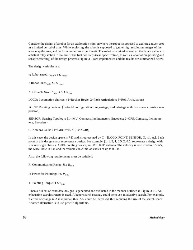
68 Methodology

Consider the design of a robot for an exploration mission where the robot is supposed to explore a given area in a limited period of time. While exploring, the robot is supposed to gather high resolution images of the area, map the area, and perform numerous experiments. The robot is required to send all the data it gathers to a distant relay station in real time. The first two steps (task specification, as well as locomotion, pointing and sensor screening) of the design process (Figure 3-1) are implemented and the results are summarized below.

The design variables are:

v: Robot speed:

l: Robot Size:

A: Obstacle Size:

LOCO: Locomotion choices: {1=Rocker-Bogie; 2=Pitch Articulation; 3=Roll Articulation}

POINT: Pointing devices: {1=Az/El configuration Single-stage; 2=dual-stage with first stage a passive sus-pension}

SENSOR: Sensing Topology: {1=IMU, Compass, Inclinometers, Encoders; 2=GPS, Compass, Inclinome-ters, Encoders}

G: Antenna Gains {1=8 dB, 2=16 dB, 3=23 dB}

In this case, the design space is 7-D and is represented by C = [LOCO, POINT, SENSOR, G, v, l, A,]. Each point in this design space represents a design. For example, [1, 1, 2, 1, 0.5, 2, 0.5] represents a design with Rocker-Bogie chassis, Az/EL pointing device, an IMU, 8 dB antenna. The velocity is restricted to 0.5 m/s, the wheel base is 2 m and the vehicle can climb obstacles of up to 0.5 m.

Also, the following requirements must be satisfied:

R: Communication Range:

P: Power for Pointing:

: Pointing Torque:

Then a full set of candidate designs is generated and evaluated in the manner outlined in Figure 3-16. An exhaustive search strategy is used. A better search strategy could be to use an adaptive search. For example,

if effect of change in A is minimal, then could be increased, thus reducing the size of the search space. Another alternative is to use genetic algorithms.

vmin v vmax≤≤

lmin l lmax≤≤

Amin A Amax≤≤

R Rmin≥

P Pmax≤

τ τ τmax≤

∆A

Methodology 69

The output of this process is a set of valid designs capable of satisfying the task specifications. The next step then is to select a single configuration for detailed evaluation.

3.5 Design Selection

A particular design from the valid set can be chosen manually based on the particular application and experience. The size of the valid set can be reduced by specifying appropriate selection requirements. For example, if the selection criterion is minimum power, then the valid set would probably result in a single design. The chosen design can then be further simulated and fine tuned. Note that the design requirements (i.e. required motion

for LOCO=(1,2,3) {

for POINT=(1,2) {

for SENSOR = (1,2) {

for {

for {

for {

for G = (1,2,3)

{

- run the configuration on terrain

- compute , P

- compute open-loop pointing error

- compute the communication range, R

if (( ) & ( ) & ( )

valid config- C = {LOCO, POINT, SENSOR, v, l, A, G}

}

}}}}}}

v vmin vmax ∆v, ,=

l lmin lmax ∆l, ,=

A Amin Amax ∆A, ,=

τ

τ τmax≤ P Pmax≤ R Rmin≥

FIGURE 3-16: Design Generation and Evaluation

Topology

Design

Evaluation

70 Methodology

ranges, rates, accelerations, torques and power) for the pointing device are automatically generated in the evaluation process. Design requirements are discussed in greater detail in Chapter 4.

3.6 Dynamic Simulation

Dynamic simulation is the final step in the design process before the pointing device is constructed. The above analysis (except some coupling metrics) is based primarily on kinematics. Kinematic analysis, although useful, cannot provide near-true indication of performance. On the other hand, dynamic analysis:

• enables analysis of the complete design along with the controller,

• facilitates designing the controller,

• allows direct coupling (dynamic) estimation/evaluation, and

• predicts near-true performance and more realistic torque/power requirements.

For the nominal case of tracking, the complete system has 8 degrees of freedom (DOF): six on the rover and two on the pointing mechanism. Dynamic modeling of an 8 DOF system is not practical due to its complex-ity; simplified models are needed. For the dynamic simulation, it is assumed that the robot is moving along the x axis in the x-z plane. The system is again reduced to 5 DOF (x,z, pitch of the vehicle and two DOF on the pointing mechanism). This model captures both linear and angular DOF on the robot, but to a reduced level. This model is valid when the vehicle is moving straight, which is true much of the time.

The dynamic model was derived using the Lewis-Abdallah-Dawson formulation [42]. The relevant equa-tions are listed in Appendix A.

The complete process of tracking system design is demonstrated in the next chapter using the example of communication from a mobile robot.

Case Study- Communication from a Mobile Robot 71

CHAPTER 4 Case Study- Communication from a Mobile Robot

Communication from mobile robots, especially outdoor mobile robots, is an impor-tant capability. The specific challenge addressed here is to achieve high data rate com-munication over an extended range (> 3-4 km) under the constraint of limited power. One method to achieve this is to use an actively pointed high gain antenna. This chap-ter presents the design of such a communication system. Tracking design was achieved using the design process outlined in the previous chapter. An antenna point-ing device was built and tested. The communication system was successfully demon-strated by achieving high data rate communication over distances greater than 10 km during the Atacama Desert Trek.

4.1 Atacama Desert Trek

The Atacama Desert Trek [5] was a planetary analogous field experiment that demon-strated several key technologies, including high bandwidth communication, necessary for robotic exploration of planets. The primary objective of the Atacama Desert Trek was to develop, demonstrate and evaluate a robot capable of long distance, long dura-tion planetary exploration. In addition to advancing robotics technologies for plane-tary exploration, the Desert Trek involved mass public participation through rich interactive video and remote operation from three distant control sites. The principal tool for enabling public participation was a high resolution panospheric camera [51].

72 Case Study- Communication from a Mobile Robot

In order to transmit the 4-6 Hz panospheric imagery from the rover to distant control sites, a high bandwidth (2 Mbps) reliable communication link was paramount.

One possible configuration uses an omnidirectional antenna to transmit data from the moving robot to a sta-tionary relay station (Figure 4-1). However, this configuration limits the rover’s maximum excursion from the relay station. This can be a major disadvantage for planetary missions because the robot must be in close proximity to the relay station and cannot explore much area. The advantage is that no pointing is required, thus simplifying the overall robot system.

The ideal scenario and initial goal was to transmit data from the rover directly to a satellite and from there to control stations [8]; however, the required size and mass of the antenna dish and transmitter equipment made this scenario unfeasible for a small exploration robot.

Therefore, it was necessary to employ a relay station. In order to expand the rover’s excursion range, the rover included a directional antenna and an antenna pointing system. The goal was to provide a communica-tion bandwidth of 1.1-1.2 Mbps over a range of 8 km.

The timing of the project made it possible to consider the complete robot in the design and development of tracking. This chapter describes the design of the high gain antenna pointing mechanism and overall track-ing system.

4.2 Task Specifications

This is the first step in the configuration process. For this task, requirements that drove the design of the tracking system included:

FIGURE 4-1: Communication Using Omnidirectional Antennas

Robot Relay Station

Control Station

Satellite Link

1-2 km

OmnidirectionalCommunication

Case Study- Communication from a Mobile Robot 73

Speed: : The lower limit is based on the minimum speed required to complete the dis-tance objective in the allotted mission duration. The objective was to complete 200 kms over 40 days. Assuming 7 hours of nominal operations per day and accounting for some downtime, the minimum speed was 0.25 m/s. The upper limit is the maximum speed of the robot on flat terrain. Tracking need not handle speeds greater than this. The goal was to configure a tracking system that would maximize this speed within these bounds.

Obstacle Height: : This is the obstacle climbing capability of the locomotion mechanism. This was based on the minimum terrain features that the robot had to traverse for the predicted terrain (based on the survey of the Atacama Terrain). The goal was to maximize the robot’s obstacle crossing capability while maintaining target tracking with the pointing mechanism.

Wheel Base: : The lower bound is based on the required stability margins of the robot (which depends on the obstacles and the slopes), while the upper bound is based on the size restriction due to transporta-tion requirements. The goal was to maximize the wheel base.

Wheel Diameter: A larger wheel diameter is normally advantageous as it provides better obstacle traversing capability. The largest diameter that can be used depends on the wheel base and the locomotion configuration. In

this work, was used for 4-wheel locomotion and for 6-wheel locomotion. The goal was to maximize the wheel diameter within these bounds. Vehicle stance was assumed to be constant (2.4m).

Communication Range: : As discussed above, direct communication between the robot and the satellite was not feasible. Another option was to communicate to a nearby relay station which could then relay the infor-mation to the satellite. It was deemed impractical to move the relay station every day (which would be required

for an omnidirectional antenna). This communication range ( ) was motivated by the need to move the relay station no more than once per week. The goal was to maximize the range while satisfying the data rate objective.

Data Rate: : Data rate was determined by the amount of data required for transporting imagery and status of the robot to control centers. The upper bound is the data rate based on the desired frame rate of images; the lower limit is obtained by increasing image compression and/or dropping the frame rate. The goal is to maximize this data rate while satisfying the communication range specification.

Power : The goal is to minimize the power required for pointing.

Target Location: . This is the elevation of the relay station with respect to ground level. The lower bound was based on the minimum elevation (based on the terrain features) required to provide line-of-sight between the payload (transmitter antenna on the robot) and the target (receiver antenna on the relay station) over the communication range. The upper bound was determined by the highest accessible elevation points in the region.

0.25m s⁄ v≤ 1.0m s⁄≤

0.25m h≤

1.8m l≤ 2.4m≤

0.4l D≤ 0.6l≤ 0.2l D≤ 0.3l≤

d 8km≥

8km≥

1.5Mbps R≤ 2.0Mbps≤

Pmax 25W Pavg 3W≤,≤

50m z≤ 200m≤

74 Case Study- Communication from a Mobile Robot

After tracking was specified, the next step was to generate the component (locomotion, pointing, state sen-sor and planner) configurations.

4.3 Screening Component Configurations

A tracking topology consists of the following components: locomotion mechanism, pointing device, sen-sors, and planner. An appropriate tracking topology consists of:

• A locomotion mechanism that minimizes the terrain disturbances transmitted to the pointing mechanism while satisfying the locomotion requirements. Vehicle Smoothing Factor (VSF) can be used to evaluate candidate locomotion configurations on the basis of terrain disturbance transmission to the pointing device. Locomotion objectives can be satisfied by choosing appropriate parameters (like wheel base, stance and diameter).

• A pointing device that is easy to control and consumes minimal power. Coupling can be used to screen pointing device configurations that isolate the payload from the locomotion, thus minimizing the motion of the pointing actuators required to keep the payload oriented towards the target.

• A set of sensors that can provide accurate state information required for control of the pointing device. Controller accuracy is limited by the accuracy of the state sensors. Sensitivity analysis can be used to cal-culate suitability of a sensor configuration for a particular task.

• A planner that emphasizes a path of minimum excursions, thus ensuring fewer disturbances to the pay-load. For the purpose of tracking, the role of path planner is to choose an appropriate velocity and avoid large obstacles.

4.3.1 Locomotion

Locomotion for unstructured environments should be very capable. The desired characteristics include a low center of gravity, good obstacle traversing capability, minimum body excursion, appropriate ground clear-ance and small turning radius. The most important functionality for tracking is body excursion. Due to their many advantages, articulated vehicle concepts are used extensively for mobile robot applications (especially for rough terrain). Articulated vehicles consist of two or more body or frame units joined together. The joints may have multiple active and passive degrees of freedom (roll, pitch, and/or yaw).

Several articulated vehicle concepts were considered. A roll articulated vehicle has an advantage in that the wheel loads are evenly distributed and can conform to terrain. Pitch articulation provides even better terrain conformability while freedom in yaw permits the use of large wheels without the need for large wheel cavi-ties in the vehicle envelope. The Rocker-Bogie concept has both roll and pitch articulation and provides low body excursions.

Case Study- Communication from a Mobile Robot 75

VSFs for a 4-wheel pitch articulated, and a Rocker-Bogie vehicle are shown in the following figure. VSF for a conventional chassis is one by definition. The data was obtained by simulating these vehicles in representative terrain (scattered obstacles, max. height- 50 cm). VSF is a strong function of different configuration, but a weak function of the dimensions of a given configuration. The following dimensions were used for calculating the VSF: 4-wheel-conventional (75 cm diameter, 1.8 m base), 4-wheel-pitch-articulation (75 cm diameter, 1.8 m wheel base), and Rocker-Bogie (38cm diameter, 1.8 m wheel base).

The average VSFs for these three configurations are: 1.00 (4-wheel-conventional), 1.49 (4-wheel-pitch-articula-tion), and 2.72 (Rocker-Bogie).

As expected, the Rocker-Bogie configuration provides fewer body excursions as compared to the other two con-figurations. Even pitch articulation is quite good. While definitely better for tracking purposes, the Rocker-Bogie is more complex (additional wheels, joints, actuators) than the pitch articulated vehicles. Both of these configura-tions were considered as potential configurations for locomotion. Because a non-articulated 4-wheel chassis has a low VSF; it was not considered further.

FIGURE 4-2: VSF for a Pitch Articulated and a Rocker-Bogie Chassis

0 10 20 30 40 50 60 70 80 90 1000.5

1

1.5

2

2.5

3

Time (s)

VS

F

Pitch ArticulationRocker−Bogie

76 Case Study- Communication from a Mobile Robot

4.3.2 Antenna Pointing Device

Several configurations for the antenna pointing mechanism were considered. In particular, two-stage point-ing [8], direct drive gimbal and gyroscopic stabilization were assessed in light of such factors as mass, power, size, cost, manufacturability, ability to use off-the-shelf components, reliability, coupling and con-trollability. A two-stage pointing device can isolate gross vehicle rotations using one mechanism (e.g., active gyroscopic stabilization or passive pendulum stabilization) and perform finer rotations with another mecha-nism (for example, a gimbal) appended to the first. While providing better performance, it was decided that two-stage pointing introduced unnecessary complexity given the low accuracy requirements of the Atacama application. Extensively used in satellite applications, gyroscopic stabilization provides better isolation of vehicle motion, but precession induced by high disturbance torques (due to vehicle motion) can be problem-atic in mobile robot applications.

For the case of a circularly polarized antenna, the beam is symmetric around its axis; therefore, orientation around the antenna’s axis is not important. In this case, at minimum only two actuators are required to orient it towards a target. So, a simple configuration of a pointing device would include two actuators. For this rea-son, only circularly polarized antennas were considered for the application. The two actuators could be arranged in an Azimuth-Elevation pattern or an X-Y pattern. Both of these configurations were evaluated by calculating kinematic coupling over representative terrains. The following values were used to compute cou-pling (See Figure 4-3.)

Coordinates of Relay Station (GPS)

Coordinates of the Vehicle (GPS)

Coordinates of the pointing mechanism in the vehicle reference frame

Kinematic coupling is shown in Figure 4-4. In this case, the average value of the kinematic coupling is approximately 0.32 for the Azimuth-Elevation configuration and more than 2.12 for the X-Y configuration. Clearly for this case, the Azimuth-Elevation configuration is superior and is therefore used to generate the tracking designs. The X-Y configuration can be screened out at this point.

4.3.3 Payload

An extensive survey was performed to find a suitable antenna for the Atacama task. The desired qualities of the antenna were high gain, flat beamwidth, low mass and low inertia. The following were chosen as poten-tial antennas:

• 8 dB 2.4 GHz, 70 deg Half Power Beamwidth, 7.0 deg pointing accuracy (based on 5% decrease in range) Flat plate, 101 x 95 x 32mm, 0.115kg

• 16dB 2.4GHz, 27 deg Half Power Beamwidth, 2.7 deg pointing accuracy (based on 5% decrease in range) Flat plate, 340 x 273 x 20mm, 1kg

xr yr zr, ,( ) 0 0 100, ,( )=

xv yv zv, ,( ) 1000 1000 0, ,( )=

xp yp zp, ,( ) 0.1 0.2 1.0, ,( )=

Case Study- Communication from a Mobile Robot 77

These were further evaluated. Also, for the sake of comparison, an omnidirectional (-3 dB 2.4 GHz) was consid-ered.

4.3.4 Sensor

Sensing configuration can be divided into the following two broad categories based on the generation of error signals for the controller:

1. Closed-loop: In this case the error is generated based on feedback from the target. For the case of wireless communication, the obvious way is to measure the strength of the signals received from the target. The criti-cal sensor in this case is the one measuring signal strength. Less critical are sensors that measure pointing actuator position.

2. Open-loop: In this case no direct feedback is received from the target. The pointing error is generated based on the known location of the target, position and orientation of the robot, as well as the orientation of the pointing device with respect to the robot.

FIGURE 4-3: Parameters for Kinematic Coupling

Relay

Station

(0, 0, 0)

(0, 0, 100)

(1000, 1000, 0)

Robot

1.0

0.1

0.2

Antenna Pointing Mechanism

78 Case Study- Communication from a Mobile Robot

When a signal strength sensing method is available, the closed-loop mode is preferable. However, for this specific case, the available radios could not provide signal strength measurements. Rather than incorporating an additional sensor, an open-loop configuration was attempted so as to make use of the state sensors avail-able on the robot. The following vector denotes the accuracy of the sensors that were available for use and required for open-loop pointing:

where

denotes the accuracy of the available GPS.

FIGURE 4-4: Kinematic Coupling

0 5 10 15 20 25 30 35 40 45 500

1

2

3

4

5

6

7

8

9

Kin

emat

ic C

oupl

ing

Time (s)

KINEMATIC COUPLING

Az/El ToplogyX/Y Topology

dx dy dz dα dβ dγ dγm dαm 30cm 30cm 30cm 1.0° 0.5° 0.5° 3.6° 3.6°·

=

dx dy dz, ,( )

Case Study- Communication from a Mobile Robot 79

denote (yaw, roll, pitch) of the vehicle and denote the accuracies of the yaw, roll and pitch sensors, respectively.

denote the positions of the elevation and azimuth motors, and are the corresponding

accuracies.

The suitability of this sensor configuration was verified using the analysis technique developed in the previous chapter.

Sensitivity Analysis: The first step in analyzing sensor configuration is to derive the inverse kinematic equa-tions. The reference frames used are shown in

{G} Global reference frame

{V} Vehicle reference frame

{A} Azimuth reference frame

{E} Elevation reference frame

The global reference frame is fixed with respect to a planet surface: its X-axis points east; Y-axis points North; and Z-axis, upwards. Since only the relative positions, and not the absolute positions, of the rover and the relay station are important, the origin of the frame is of minor importance. The Y-axis of the vehicle reference frame points forward; the X-axis points to the right side of the vehicle; the Z-axis points up. The vehicle frame is located at the vehicle’s center of gravity. Azimuth {A} and Elevation {E} are the two frames associated with the

α β γ, ,( ) dα dβ dγ, ,( )

γm αm,( ) dγm dαm,( )

FIGURE 4-5: Reference Frames

{G}

{V}

{A}{E}Y

X

Z

Xv

Yv

Zv

YA

YE

XA XE

ZE

ZA

Robot

Mast

Antenna PointingMechanism

80 Case Study- Communication from a Mobile Robot

antenna pointing mechanism. The origins of these two frames are coincident and located at the intersection of the azimuth and elevation actuator axes. The Z-axis of the azimuth frame is normal to the vehicle pointing upwards; the y-axis is pointed in the direction of vehicle travel. This frame is parallel to the vehicle frame. The elevation frame is obtained by rotating the azimuth frame around the azimuth Z-axis by , the azimuth

angle. The standard z-y-x Euler angle representation is used for the analysis. The required azimuth and ele-vation angles for line-of-sight pointing are given by:

and

where are defined as

Here,

Required Azimuth Angle (Encoder)

Required Elevation Angle (Encoder)

Coordinates of Relay Station (GPS)

Coordinates of the Vehicle (GPS)

Coordinates of the pointing mechanism in the vehicle reference frame

The output error in azimuth and elevation are and , respectively. In these

equations and are the actual azimuth and elevation of the payload. They are obtained by dividing the motor positions by the appropriate gear ratios. Thus

and .

γp

αp X Y⁄–( )atan= γp Z X2

Y2+ ⁄

atan=

X Y Z, ,

X xp– xr xv–( ) αcos βcos yr yv–( ) α βcossin zr zv–( )– βsin+ +=

Y yp– xr xv–( ) α β γsinsincos α γcossin–{ } yr yv–( ) α γcoscos α β γsinsinsin+{ } zr zv–( ) β γsincos+ + +=

Z zp– xr xv–( ) α β γcossincos α γsinsin+{ } yr yv–( ) α β γcossinsin α γsincos–{ } zr zv–( ) β γcoscos+ + +=

αp

γp

xr yr zr, ,( )

xv yv zv, ,( )

xp yp zp, ,( )

eα αp αactual–= eγ γp γactual–=

αactual γactual

αactual αm Nα⁄= γactual γm Nγ⁄=

Case Study- Communication from a Mobile Robot 81

and are the gear reduction ratios for azimuth and elevation assemblies respectively. The error analysis

was performed by differentiating the expressions for and as:

, where is the total estimated azimuth error due to all sensors and

is the estimated azimuth error due to the sensor. Similarly,

where is the vector representing all the sensor values.

The total pointing error, , is related to and by

The sensor criticalities, s, and configuration suitability, S, can be evaluated as defined in the previous chapter.

and

where

Criticality of sensor

Total pointing error due to sensor,

Total allowable pointing error

The analysis was performed by simulating the robot over a representative terrain. The following sinusoids were used for left wheels and right wheels respectively:

Nα Nγ

eα eγ

eαeα∂qj∂-------- qjd

j

∑ eα jˆ

j

∑= = eα

eα j

eα∂qj∂-------- qjd= j

th

e γeγ∂qj∂------- qjd

j

∑ eγjˆ

j

∑= =

q xr yr zr x, , , v yv zv α β γ αm γm, , , , , , ,[ ]=

eT eα eγ

eT γp2eα

2eγ

2+=

Cj

Cj maxeTj

emax----------

= S maxeT

emax----------

=

Cj jth

eTj jth eTj γp2eα j

2 eγj2+=

emax

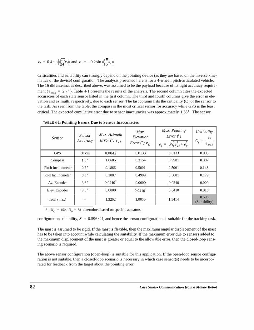
82 Case Study- Communication from a Mobile Robot

and

Criticalities and suitability can strongly depend on the pointing device (as they are based on the inverse kine-matics of the device) configuration. The analysis presented here is for a 4-wheel, pitch-articulated vehicle. The 16 dB antenna, as described above, was assumed to be the payload because of its tight accuracy require-

ment ( ). Table 4-1 presents the results of the analysis. The second column cites the expected accuracies of each state sensor listed in the first column. The third and fourth columns give the error in ele-vation and azimuth, respectively, due to each sensor. The last column lists the criticality (C) of the sensor to the task. As seen from the table, the compass is the most critical sensor for accuracy while GPS is the least critical. The expected cumulative error due to sensor inaccuracies was approximately . The sensor

configuration suitability, , and hence the sensor configuration, is suitable for the tracking task.

The mast is assumed to be rigid. If the mast is flexible, then the maximum angular displacement of the mast has to be taken into account while calculating the suitability. If the maximum error due to sensors added to the maximum displacement of the mast is greater or equal to the allowable error, then the closed-loop sens-ing scenario is required.

The above sensor configuration (open-loop) is suitable for this application. If the open-loop sensor configu-ration is not suitable, then a closed-loop scenario is necessary in which case sensor(s) needs to be incorpo-rated for feedback from the target about the pointing error.

*. , determined based on specific actuators.

TABLE 4-1: Pointing Errors Due to Sensor Inaccuracies

SensorSensor

Accuracy

Max. Azimuth

Error ( )

Max. Elevation

Error ( )

Max. Pointing

Error ( )Criticality

GPS 30 cm 0.0042 0.0133 0.0133 0.005

Compass 1.0685 0.3154 0.9981 0.387

Pitch Inclinometer 0.1866 0.5001 0.5001 0.143

Roll Inclinometer 0.1087 0.4999 0.5001 0.179

Az. Encoder 0.0240* 0.0000 0.0240 0.009

Elev. Encoder 0.0000 0.0410* 0.0410 0.016

Total (max) - 1.3262 1.0050 1.54140.596

(Suitability)

zl 0.42π24------xl

sin= zr 0.2–2π16------xr

sin=

emax 2.7°=

1.55°

° eα j ° eγj

°

ej γp2eα j

2eγ j

2+=

Cj

ej

emax----------=

1.0°

0.5°

0.5°

3.6°

Nα 150= Nγ 88=

3.6°

S 0.596 1≤=

Case Study- Communication from a Mobile Robot 83

4.3.5 Planner

Morphin [63] was the only planner available for Nomad1. Fortunately, Morphin is appropriate for this research. After considering hazards, it determines a safe speed and path for the robot. Although not implemented, a track-ing hazard module could be added that would assign a high hazard value to any path unsuitable for tracking (e.g., large obstacle, a dense obstacle field).

4.4 Tracking Design- Synthesis and Evaluation

In this case the configuration space is 8-D (LOCO, POINT, ANTENNA, v, l, D, h, ) such that,

, where LOCO =1 represents a 4-wheel pitch articulation configuration, and LOCO = 2 denotes a 6-wheel Rocker-Bogie configuration,

, where POINT=1 denotes a Az/El configuration,

, where ANTENNA=1 denotes the 8dB gain antenna, and ANTENNA=2 represents the 16 dB gain antenna, and

, the wavelength of the sinusoid, denotes obstacle distribution. Thus, the vehicle should be able to traverse one step every fifteen vehicle-lengths at a minimum, up to one step for every five vehicle-lengths.

As discussed in the task specifications:

v:

l:

D:

h: .

Each point in this 8-dimensional configuration space is a design. In other words, a design is generated by assign-

ing values to each of the variables (LOCO, POINT, ANTENNA, v, l, D, h, ).

1. The robot developed for the Atacama Desert Trek was named Nomad.

λ

LOCO 1 2,{ }∈

POINT 1{ }∈

ANTENNA 1 2,{ }∈

λ 5l 15l,[ ]=

0.25m s⁄ v≤ 1.0m s⁄≤ ∆v 0.25m s⁄=

1.8m l≤ 2.4m≤ ∆l 0.2m=

0.4l D≤ 0.6l≤ ∆D 0.1l=

0.25m h≤ 0.55m≤ ∆h 0.05m=

λ

84 Case Study- Communication from a Mobile Robot

For example, (1,1,1,0.25, 1.6, 0.8, 0.4, 16) represents a tracking design. This design represents a 4-wheel pitch articulated chassis, with a wheel base of 1.6 m and diameter of 0.8m. It can travel up to maximum speed of 0.25 m/s and can traverse steps of up to 40 cm height. Approximate obstacle distribution is one step (40 cm height) every 16m of traverse. It uses an Az/El pointing configuration. (2,1,1,0.25, 1.6, 0.8, 0.4, 16) represents another design that is based on a 4-wheel articulated chassis. Everything else remains the same as for the previous case.

The designs were evaluated by simulating the motion over a sinusoidal terrain (Figure 4-6). Each side of the wheel traversed a different sinusoid. The initial position of the vehicle was assumed to be (1000m, 1000m, 0) while the target was fixed at (0, 0, 1000m) in some fixed frame. The robot was assumed to be moving at a

commanded speed, v. A fixed yaw rate ( rad/s) was also imposed on the robot by virtue of the terrain and the speed.

A design was considered valid if all of the following conditions were satisfied:

Communication Range

Sensor Suitability

Pointing Power &

So, a valid design is a point, (LOCO, POINT, ANTENNA, v, l, D, h, ), in the configuration space such that all of the above conditions are satisfied.

π 4⁄

d 8km≥

S 0.80≤

PAZ 2.0W≤ PEl 0.15W≤

λ

Case Study- Communication from a Mobile Robot 85

FIGURE 4-6: Terrain

lambda = 18 m

l = 1.8m

A = 0.37m

D=0.75m

Left wheelsRight wheels

86 Case Study- Communication from a Mobile Robot

The evaluation of the complete configuration space (2592 designs) resulted in 78 valid designs. Some of the more interesting ones are shown in Table 4-2. These designs are either for high travel speed or large steps.

Notice that azimuth torques and power are similar for all these configurations. This is expected as all the configurations are experiencing the same yaw. None of the 8dB antenna passed as valid designs.

2592 designs were generated during the evaluation process. Without using VSF or coupling for screening (meaning considering the conventional chassis and X-Y Pointing as well), 7776 designs would have been generated. As more component configurations are considered, VSF, coupling, and suitability eliminate more unsuitable options. This can save considerable computing time. In particular, for search using genetic algo-rithms these metrics provide appropriate measure to evaluate configurations, and hence guide the search of the design space.

For comparison purposes, designs were also generated using a conventional chassis and an X-Y pointing device in a separate simulation. Tracking with a 4-wheel conventional chassis and/or X-Y pointing configu-

*. Average over the course of terrain

TABLE 4-2: Valid Designs

No.Valid DesignC = [L, P, A, v, l, R, h, ]

Power (W) Torque (N-m) Comm Range (Km)

SensorSuitability

Avg.* Coupling

Avg.* VSFAz El Az El

1 [1, 1, 3, 0.75, 2, 0.5, 0.5, 30] 1.96 0.11 2.05 0.57 10.2 0.42 0.33 1.58

2 [1, 1, 3, 0.75, 2.4, 0.48, 0.48, 36] 1.96 0.11 2.04 0.55 10.2 0.41 0.33 1.52

3 [1, 1, 3, 1, 2.4, 0.45, 0.45, 18] 1.96 0.15 2.04 0.6 10.2 0.4 0.33 1.32

4 [1, 1, 3, 1, 2.4, 0.40 0.48, 36] 1.96 0.13 2.04 0.6 10.2 0.41 0.32 1.68

5 [2, 1, 3, 0.75, 1.8, 0.27, 0.54, 18] 1.96 0.1 2.04 0.58 10.2 0.4 0.33 2.47

6 [2, 1, 3,0.75, 2, 0.25, 0.5, 10] 1.96 0.15 2.05 0. 10.2 0.39 0.32 2.33

7 [2, 1, 3, 0.75, 2.2, 0.28, 0.55, 22] 1.96 0.1 2.05 0.56 10.2 0.4 0.33 3.07

8 [2, 1, 3, 1, 1.8, 0.23, 0.45, 18] 1.96 0.08 2.04 0.53 10.2 0.38 0.32 2.41

9 [2, 1, 3, 1, 2.4, 0.24, 0.48, 36] 1.96 0.07 2.04 0.46 10.2 0.39 0.32 2.51

λ

Case Study- Communication from a Mobile Robot 87

ration required high torque/power and were valid only for lower speeds and obstacle heights. The following table shows some invalid designs:

In this table, the first design is based on the 8 dB gain antenna. The communication range in this case is 4.08 km, which is less than desirable. All of the designs based on the 8 dB gain antenna were invalid for this reason. The second design is based on an X-Y pointing configuration. In this case, the torques and power are very high and so the designs did not qualify. This was already expected based on the coupling value. The high coupling (and suit-ability) value indicates that the mechanism operates near singular configuration. The third design, based on the conventional 4-wheel chassis, did not qualify because of small traversable obstacle sizes. For larger obstacles, the power required is more than the limit.

4.5 Design Selection

The next step is the design selection. As is clear from Table 4-2, there are only two valid topologies- one uses a 4-wheel pitch articulated vehicle, and the other has a 6-wheel Rocker-Bogie chassis. Both these use Az/El point-ing for orienting the 16dB antenna. As a result, choosing either the 4-wheel pitch articulated vehicle or the Rocker-Bogie chassis was a central decision.

One of the main objectives was to maximize speed. The maximum speed of 1.0 m/s corresponds to design-4 and design-9 for pitch articulation and Rocker-Bogie respectively. The corresponding rows from Table 4-5 are copied below:

TABLE 4-3: Some Invalid Designs

S. No. C = [L, P, A, v, l, R, h, ]

Power (W) Torque (N-m)Comm Range (Km)

SensorSuitability

Avg. Coupling

Avg. VSFAz El Az El

1 [2, 1, 2, 0.25, 1.8, 0.18, 0.18, 9] 1.72 0.01 1.79 0.11 4.08 0.13 0.29 2.45

2 [2, 2, 3, 0.25, 1.8, 0.18, 0.18, 9] 5.84 2.87 1.98 3.43 10.2 98.5 207 2.52

3 [3, 1, 3, 0.5, 1.8, 0.36, 0.18, 9] 1.71 0.05 1.79 0.20 10.2 0.13 0.30 1.00

No.Valid DesignC = [L, P, A, v, l, R, h, ] Power (W) Torque (N-m)

Comm Range (Km)

SensorSuitability

Avg. Coupling

Avg. VSF

4 [1, 1, 3, 1, 2.4, 0.40 0.48, 36] 1.96 0.13 2.04 0.6 10.2 0.41 0.32 1.68

9 [2, 1, 3, 1, 2.4, 0.24, 0.48, 36] 1.96 0.07 2.04 0.46 10.2 0.39 0.32 2.51

λ

λ

88 Case Study- Communication from a Mobile Robot

The Rocker-Bogie has a slight advantage in torque and power. But the major portion of power consumption is in the azimuth actuator (approximately 4 times that of elevation) and Rocker-Bogie does not provide any advantage there over the pitch-articulation. Neither the Rocker-Bogie nor the pitch-articulated vehicle has a yaw averaging capability. Although the Rocker-Bogie consumes less power for tracking, it is more complex than a 4-wheel articulated vehicle (2 additional wheels, more linkages, possibly more actuators). The power savings were judged to not be worth the added complexity and so design-4 was chosen for further develop-ment.

This does not mean that the Rocker-Bogie would only be minimally superior for other tracking applications. For applications where azimuth is not key (e.g., tracking an overhead target) the Rocker-Bogie would be much better.

4.6 Dynamic Simulation

The objective here is to design a simple controller that meets the tracking requirements. A dynamic model as detailed in Appendix A was used for the simulation. To begin, a PID control and a computed torque control were implemented. Figure 4-7 shows some performance graphs for a PID controller. The graph shows point-ing errors (azimuth and elevation) in the presence of two types of disturbance inputs (rover pitch)- an impulse input and a sinusoidal input. As is clear from the graphs, the nominal pointing error is quite small

(less than ).

Similar simulations were performed using computed torque strategy. The computed torque control per-formed better (nominal errors- ~ ) than the PID controller. However, the performance improvement is

minimal compared to the error due to sensors ( ), derived in earlier sections. Also, the computed torque control is very susceptible to modeling errors.

The combined error due to the sensors ( ) and PID controller ( ) is , which is within the allowable range ( ). Since the errors are within the allowable margin, and PID control is easier to imple-ment, it was selected as the control strategy.

4.7 Detailed Design

The final design chosen was [1, 1, 3, 1, 2.4, 0.40 0.48, 36], which implies a pitch-articulated chassis with an Az/El point-ing device. The wheel base is about 2.4 m and the wheel diameters are 0.8 m. The tracking can handle obstacles up to 40 cm in height while traversing at 1 m/s horizontal speed. The following sections discuss the design in detail.

0.2°

0.1°1.55°

1.55° 0.2° 1.75°2.7°

Case Study- Communication from a Mobile Robot 89

0 0.5 1 1.5 2 2.5 3 3.5 4 4.5 5 5.5−2

−1.5

−1

−0.5

0

0.5

1

1.5

2

time (s)

erro

r (d

eg)

PID Control, Sinusoidal Input

0 0.5 1 1.5 2 2.5 3 3.5 4 4.5 5 5.5−5

−4

−3

−2

−1

0

1

2

3

4

5

time (s)

erro

r (d

eg)

PID Control, Impulse InputImpulse Disturbance Input

Poi

nti

ng O

ffse

t (d

eg)

Poi

nti

ng O

ffse

t (d

eg)

Sinusoidal Disturbance Input

Time (s)

Time (s)

Azimuth Offset

Elevation Offset

Azimuth Offset

Elevation Offset

FIGURE 4-7: PID Control- Pointing Offset Vs. Time

90 Case Study- Communication from a Mobile Robot

4.7.1 Locomotion

Nomad’s chassis is pitch articulated [5] (Figure 4-8). The two wheels on each side of the robot are attached to a bogie which pitches relative to the body about a central axis. This ensures that all four wheels are always in contact with the ground. With the pivot placed in the middle of each bogie, the vertical excursion of the pivot is the average vertical excursion of that bogie’s two wheels. Since this happens on both sides of the vehicle, the average pitch of the body is fixed at the average of the pitches of two bogies. The wheels are 76.2 cm in diameter and each wheel is individually powered.

Nomad’s chassis (Figure 4-9) expands, compacts, and steers by driving a pair of four-bar mechanisms on either side of the robot. In the “deployed” mode, Nomad’s stability and propulsion over variable terrain are drastically improved. The nominal wheel base of 2.4 m reduces to 1.8 m in the compact mode.

4.7.2 Antenna Pointing Mechanism

The antenna pointing based on the result of the design process is a single stage Az/El device. Once the con-figuration is fixed, the next step, before building the device, is to derive the performance requirements.

Requirements. The specifications required are the excursions and rates required for tracking, and the mass and size of the payload. Now, elevation range is a combination of three factors:

• Motion of the rover, e.g., rocking and turning

• Terrain characteristics, e.g., slopes and steps

• Distance from the relay station

FIGURE 4-8: Nomad’s Pitch Articulated Chassis

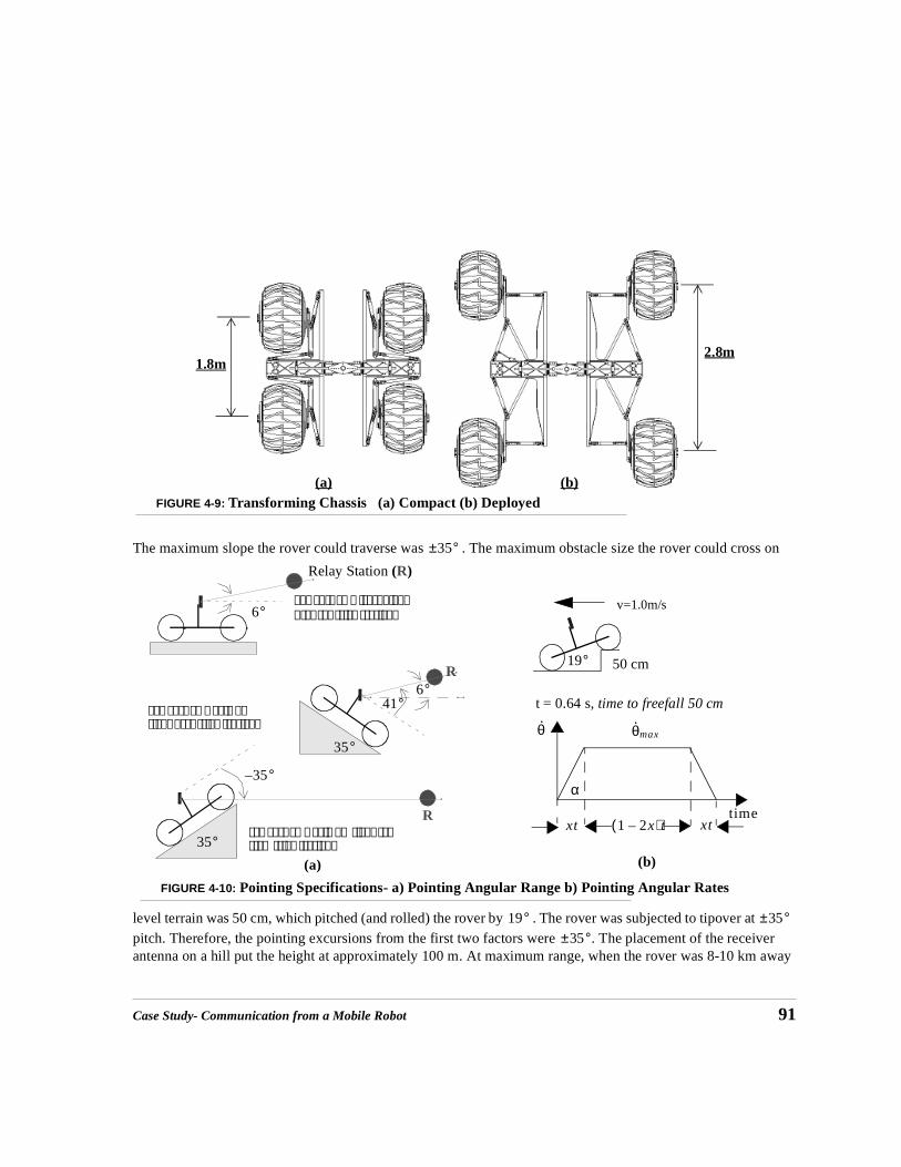
Case Study- Communication from a Mobile Robot 91

The maximum slope the rover could traverse was . The maximum obstacle size the rover could cross on

level terrain was 50 cm, which pitched (and rolled) the rover by . The rover was subjected to tipover at pitch. Therefore, the pointing excursions from the first two factors were . The placement of the receiver antenna on a hill put the height at approximately 100 m. At maximum range, when the rover was 8-10 km away

FIGURE 4-9: Transforming Chassis (a) Compact (b) Deployed(a) (b)

2.8m1.8m

35°±

35– °

35°

35°

6°

6°

41°

Relay Station (R)

R

R

a) Rover on a level planenear the relay station.

b) Rover on maximumslope near relay station.

c) Rover on maximum slope farfrom relay station.

(a)

FIGURE 4-10: Pointing Specifications- a) Pointing Angular Range b) Pointing Angular Rates

50 cm19°

t = 0.64 s, time to freefall 50 cm

v=1.0m/s

(b)

θ·

time

α

θ·max

xt xt1 2x–( )t

19° 35°±35°±

92 Case Study- Communication from a Mobile Robot

from the receiver antenna, the elevation angle of the antenna with the rover on flat ground was effectively

zero. Restricting the minimum range to 1 km, the corresponding angle was approximately . As shown in Figure 4-10a, the required total elevation was to + . Including a safety factor, the antenna pointing

mechanism was specified for to + . The azimuth specified was continuous.

The elevation rate was approximated as the rate at which the angle changes when the robot falls from a 50 cm step (Figure 4-10b). The rates and accelerations shown in Table 4-4 are based on a trapezoidal velocity profile (Figure 4-10b) and include a safety factor.

The pointing accuracy, payload mass, and payload size in the above table is specified for the 16 dB antenna chosen during the design process. The requirements for the APM are tabulated above. The following table gives specifications of some other antenna pointing systems for comparison. Toshiba APM-1 [34] and HST STAPS [34] are antenna positioners for satellite applications while KVH’s TracVision [74] is for antenna pointing from boats. As seen from the table, the pointing rates for these applications are much lower than the rates required for the mobile robot pointing task described in this chapter; therefore they are not useful here.

TABLE 4-4: Antenna Pointing Requirements

Item Value

Elevation range to +

Azimuth range continuous

Elevation Rate

Azimuth Rate

Elevation Acceleration

Pointing Accuracy

Payload Mass 2 kg

Payload Size 27.3 x 34 x 2 cm

TABLE 4-5: Comparison of Various Antenna Pointing Mechanisms

ToshibaAPM-1

HST STAPS KVHTracVision

CMU(objective)

Configuration X-Y X-Y Az/EL Az/EL

Excursion( )+/- 15 both axes

+/- 110 x+/- 110 y

+/- 110 ElAz. Cont.

+/- 60 ElAz. Cont.

Rate ( ) 0.31 0.5 12 75

Mass (kg) 9.90 17.2 10.1 10*

6°35°– 41°

40°– 60°

40°– 60°

75° s⁄

30° s⁄

3000° s2⁄

2.7°

°

° s⁄

Case Study- Communication from a Mobile Robot 93

The final configuration chosen and developed was a single stage, 2-dof mechanism with brushed actuator and harmonic drive reducer. Figure 4-11 shows the configuration. The main features of the mechanism are:

1. Azimuth/Elevation configuration: The mechanism consists of an azimuth and an elevation assembly. The ele-vation actuator lies above the azimuth actuator. This configuration has less coupling (dynamic and kinematic) compared to the X-Y configuration for the given Atacama mission scenario.

2. Slip ring for elevation actuator: A slip ring is used for power, sensing (encoder signal) and command of the elevation actuator. Slip rings, although considered more complex and less reliable than cable wraps, are suit-able for this application for several reasons. A slip ring:

• allows continuous rotation, unlike a cable wrap.

*. Based on the initial mass and power budgets.

Power (W)39 Peak, 4.5 Avg

30 Nominal54 Peak28 Nom

25*

Accuracy ( ) 0.0029 0.6 3 2.7

TABLE 4-5: Comparison of Various Antenna Pointing Mechanisms

ToshibaAPM-1

HST STAPS KVHTracVision

CMU(objective)

°

Antenna

Counter Mass

Elevation Actuator

Azimuth Assembly

Slip Ring/RF Joint Assembly

FIGURE 4-11: Antenna Pointing Mechanism

94 Case Study- Communication from a Mobile Robot

• reduces size because management of cables to avoid minimum bend radii (of RF flexible cable and other wires) is difficult in a compact package.

• does not introduce unpredictable and/or variable resistant torques, which are inherent in a cable wrap solution.

3. RF rotary joint: An RF rotary joint is used to send RF signals from the transmitter to the antenna. The RF rotary joint is co-axial with the slip ring. The RF rotary joint has certain advantages over flexible cable:

• The RF characteristics remain nearly constant. With flexible cable, the RF characteristics change ran-domly with cable motion.

• A RF rotary joint introduces fewer losses. Typical loss in flexible RF cable is about 0.2 dB/ft. Total loss using cable wrap is about 1.2 dB compared to 0.5 dB for RF rotary joint.

4. Harmonic drive and brushed motor: Brushed motors are used with harmonic reduction for both azimuth and elevation actuators. The primary rationale was to minimize backlash. A typical off-the-shelf plane-

tary gear train has a backlash about of , which is unsuitable for the application.

5. Balanced system: The payload is balanced using a counter mass. This minimizes disturbance torques, thus reducing the size of the actuators and complexity of the controller.

This configuration using RF rotary joint, slip rings and balanced payload proved to be suitable for this appli-cation.

4.7.3 State Sensors

As discussed earlier, an open-loop control strategy is suitable for the task. Several state sensors are needed to measure the position of the receiver antenna, robot position, and robot orientation as well as azimuth and elevation angles. The following sensors were used for antenna pointing:

• DGPS: A Differential Global Positioning System was used to derive the positions of the robot and the relay station in the inertial frame. One GPS unit was mounted on the rover, another (the master unit) at the relay station. The two receivers were used in a differential configuration to provide good position accuracy.

• Compass: A stabilized gyro compass was used to measure the magnetic azimuth of the vehicle.

• Inclinometers: Inclinometers were used to measure the roll and pitch of the vehicle.

• Encoders: Incremental encoders mounted on the motors were used to sense the positions of azimuth and elevation motors. Optical switches were used on the output end of azimuth and elevation gear trains to generate an absolute signal for indexing.

The result of sensitivity analysis on this configuration is presented in Table 4-1. The maximum pointing error due to the sensors is approximately , which is 60% of the total allowable error. So, the controller

error, even in the worst case, should not exceed (40% of the total allowable error).

1° 2°–

1.55°1.15°

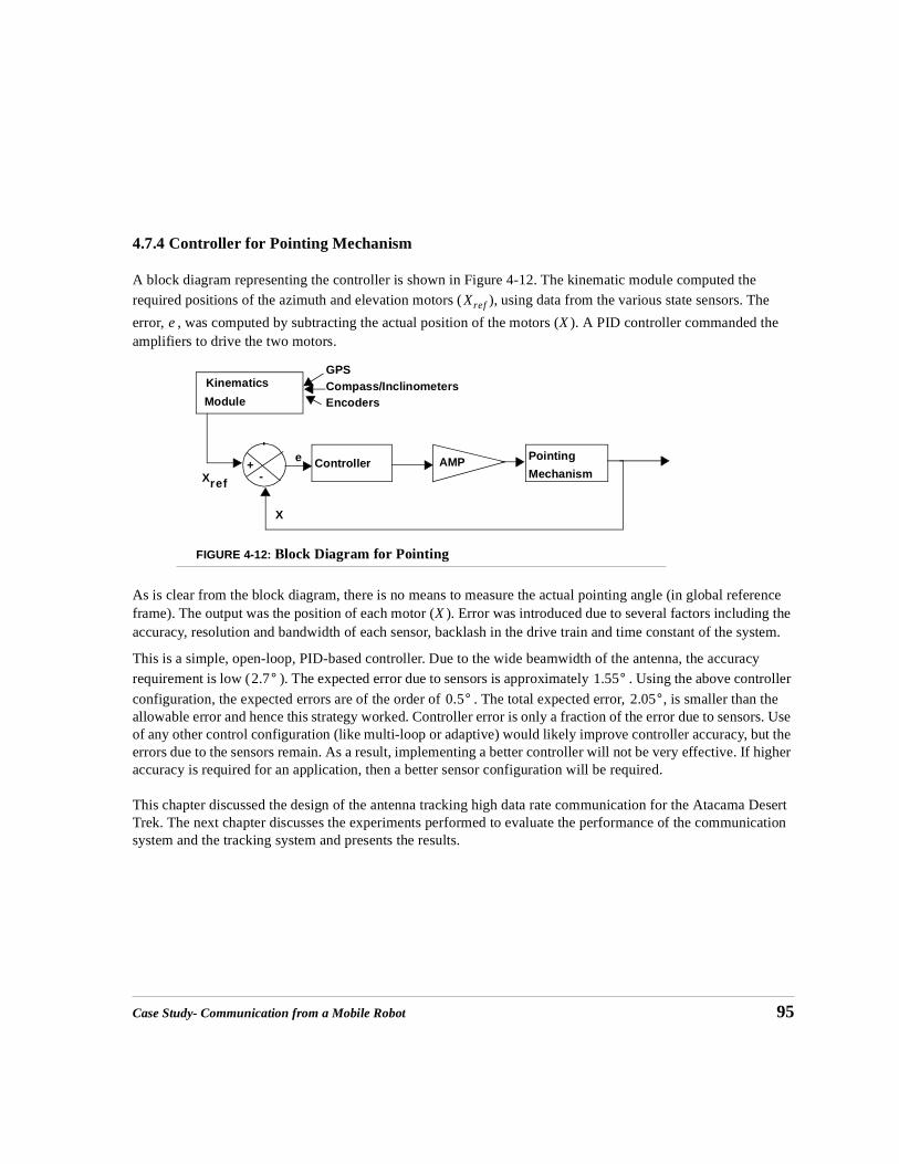
Case Study- Communication from a Mobile Robot 95

4.7.4 Controller for Pointing Mechanism

A block diagram representing the controller is shown in Figure 4-12. The kinematic module computed the required positions of the azimuth and elevation motors ( ), using data from the various state sensors. The

error, , was computed by subtracting the actual position of the motors ( ). A PID controller commanded the amplifiers to drive the two motors.

As is clear from the block diagram, there is no means to measure the actual pointing angle (in global reference frame). The output was the position of each motor ( ). Error was introduced due to several factors including the accuracy, resolution and bandwidth of each sensor, backlash in the drive train and time constant of the system.

This is a simple, open-loop, PID-based controller. Due to the wide beamwidth of the antenna, the accuracy requirement is low ( ). The expected error due to sensors is approximately . Using the above controller

configuration, the expected errors are of the order of . The total expected error, , is smaller than the allowable error and hence this strategy worked. Controller error is only a fraction of the error due to sensors. Use of any other control configuration (like multi-loop or adaptive) would likely improve controller accuracy, but the errors due to the sensors remain. As a result, implementing a better controller will not be very effective. If higher accuracy is required for an application, then a better sensor configuration will be required.

This chapter discussed the design of the antenna tracking high data rate communication for the Atacama Desert Trek. The next chapter discusses the experiments performed to evaluate the performance of the communication system and the tracking system and presents the results.

Xref

e X

FIGURE 4-12: Block Diagram for Pointing

Kinematics

Module

+-

Controller AMP Pointing

Mechanism

GPSCompass/InclinometersEncoders

Xref

X

e

X

2.7° 1.55°0.5° 2.05°

96 Case Study- Communication from a Mobile Robot

Experiments 96

CHAPTER 5 Experiments

Experiments were performed during the final demonstration of the Atacama Desert Trek to evaluate the performance of the communication link and the pointing device. The main objectives of the experiments were:

Objective 1: Long Range Communication. Long range communication at a high data rate is an important capability for outdoor mobile robots and was one of the main fea-tures tested during the Atacama Desert Trek. The objective of this particular experi-ment was to determine the maximum range over which the communication link could deliver the required data rate from the robot while moving over various types of natu-ral terrain.

Objective 2: Performance Quantification. This research quantifies the influence of various robot parameters on tracking system design performance for mobile robot applications. The objectives of these experiments were to study the effect of the parameter variations on the pointing performance and to verify the results obtained in previous chapters.

97 Experiments

5.1 Long Range Communication

The communication scenario for the desert trek was to transmit data from the robot to a relay station, which would then relay the data back to a satellite truck. (The satellite truck subsequently relayed the data to the remote control station using a satellite link.) A principal objective was to maximize the distance between the robot and the relay station, thus minimizing the number of relay stations required.

A system-level long range communication test was performed by starting the robot near a relay station (~200 m) and then allowing it to travel as far as possible, so long as there was no appreciable degradation in the data rate (Figure 5-1). During the course of the several day experiment, the robot moved over diverse ter-rains (soft and hard, with different sizes, shapes, and distribution of obstacles) of the Atacama desert, at a range of speeds (up to 40 cm/s). During the test, the vehicle disturbance rates (roll/pitch/yaw rates) were up

to . The data rate, although not directly measured, was qualitatively judged on the basis of the high resolution images received at the control stations. The robot was allowed to move farther and farther from the relay station as long as complete images were received at the remote control stations.

25° s⁄

FIGURE 5-1: Long Range Communication Experiment

100m

~0.2-11km

Relay Station

Experiments 98

During this experiment, several communication drop outs occurred, but they were primarily due to line-of-sight occlusions. The radio used could operate only when in line-of-sight of the hilltop relay station. The antenna pointing mechanism performed without failure and enabled communication at ranges of up to 11 km- to our knowledge, a record for this class of machines. These results also agree with the simulation results presented in Chapter 3, which predicted a 10.2 km range.

5.2 Performance Quantification

The objectives of these experiments were to study the effects of various parameters (speed, turn radius, obstacle heights, and wheel base) on the pointing performance and to verify the results obtained in the previous chapters. In all cases, the pointing was maintained to enable a constant communication link. As discussed below, this link was actually used to log the experimental data. One limitation of the experiment, which is described in a section below, is that no direct measure of antenna pointing accuracy with respect to the target was available. Therefore, pointing error was inferred from sensor performance predictions and measured servo errors.

5.2.1 Experimental Setup

The tests were performed in the Atacama Desert, Chile, during experiments with the Nomad robot. The test ter-rain was located approximately 1 km from the relay station. The height of the relay station with respect to the test terrain was 100 m (Figure 5-2). The ground was mostly flat and covered with small pebbles with soft terrain beneath.

~1000m

100m

FIGURE 5-2: Experimental Setup

99 Experiments

All the tests were performed in the same region. Although the intention was to move the robot over identical paths for all the tests, slight variations occurred due to the slippage of the robot’s wheels from one circuit to the next. This is clear from the sample GPS plot shown in Figure 5-3. For this experiment, the robot was commanded to traverse a circle with a radius of 8 m twice.

For the tests, Nomad was commanded remotely, either from the relay station or local control station, to drive at a specific speed along a specific path. The test data was also logged remotely at the local control station. The data was logged in Matlab format for easy analysis.

5.2.2 Data Logged

The following parameters were changed in a controlled manner (Table 5-1): obstacle size, vehicle speed, turning radius, and wheel base.

TABLE 5-1: Variables for the Pointing Experiments

VariableNominal

ValueRange of Values Comments

Vehicle Speed (m/s) 0.3 0.15, 0.3,0.4 These are commanded speeds and might be slightly different from the actual speed.

Turning Radius (m) 8 4, 8, 12 At constant speed, this is equivalent to vary-ing the vehicle yaw rate.

FIGURE 5-3: GPS Plot

1355 1360 1365 1370

−90

−88

−86

−84

−82

−80

−78

−76

X (m)

Y (

m)

Experiments 100

The following data were collected during each experiment.

Obstacle Size (cm) 0 (flat terrain) 0, 12.5, 17.5, 25.0 Obstacles were not exact steps. This is the height at the highest point.

Wheel Base (m) 2.4 1.8, 2.4 1.8 m is wheelbase for the most compact configuration and 2.4 m is the wheelbase for the deployed configuration

TABLE 5-2: Data Logged During the Experiments

Item Units Sensor Notation

X coordinate of the robot with respect to the relay station m DGPS X

Y coordinate of the robot with respect to the relay station m DGPS Y

Z coordinate of the robot with respect to the relay station m DGPS Z

Roll of the robot rad AGDC

Pitch of the robot rad AGDC

Yaw of the robot rad AGDC

Current azimuth of the antenna rad Azimuth Motor Encoder

Current elevation of the antenna rad Elevation Motor Encoder

Desired azimuth of the antenna rad Inverse Kinematic

Desired elevation of the antenna rad Inverse Kinematic

Command to azimuth amplifier Volts Controller (software)

Command to elevation amplifier Volts Controller (software)

Command to each wheel amplifier Volts Controller (software) ,

Time msec System clock t

TABLE 5-1: Variables for the Pointing Experiments

VariableNominal

ValueRange of Values Comments

φ

θ

ψ

α

γ

α0

γ0

cα

cγ

co c1,

c2 c3,

101 Experiments

5.2.3 Derivation of the Performance Parameters

For the pointing device, the specific variables of interest are torque, power and error. These were computed from the data in Table 5-2 using the method shown below.

Azimuth and elevation torques. The azimuth and elevation torques, and , were computed using the

commands, and , to the azimuth and elevation actuators.

where

amplifier gain for the azimuth amplifier

torque constant for the azimuth actuator.

Similarly,

where

amplifier gain for the elevation amplifier

torque constant for the elevation actuator.

As is clear from the above computations, the torques are computed using the commanded signal. The actual measurement of either the current to the motors or torque was not available; hence, the indirect approach was used. The amplifier gain formula was however verified from an isolated motor/amplifier test. Figure 5-4 shows the results of one such test, when the motor was first commanded to move counterclockwise and then clockwise at the maximum speed. Both the commanded current and the actual current were recorded. As is clear from the graph, they match fairly closely.

Azimuth and elevation power. As robots are usually limited in power, power is one of the key performance parameters for pointing tasks from mobile robots. The power for the pointing device was computed as:

τα τγ

cα cγ

τα aαcαkα=

aα 0.8Amp

V-----------=

kα 2.46Nm

Amp-----------=

τγ aγcγkγ=

aγ 0.8Amp

V-----------=

kγ 5.08Nm

Amp-----------=

Experiments 102

where,

azimuth pointing power

voltage across the azimuth actuator

current for the azimuth actuator

, voltage constant for the azimuth actuator.

Similarly,

where

elevation pointing power

0 2 4 6 8 10 12 14 16 18−0.5

−0.4

−0.3

−0.2

−0.1

0

0.1

0.2

0.3

0.4

0.5

Time (s)

Cur

rent

(A

mps

)

Commanded CurrentActual Current

FIGURE 5-4: Commanded Current vs. Monitored Current

Pα VαIα Kvαα·( ) aαcα( )= =

Pα

Vα

Iα

Kvα 0.26V

rpm----------

7.8π-------

Vrad s⁄---------------= =

Pγ VγIγ Kvγγ·( ) aγcγ( )= =

Pγ

103 Experiments

voltage across the elevation actuator

current for the elevation actuator

voltage constant for the elevation actuator.

As for the torque, the direct measurements of the power (or current and voltage) were not available: the val-ues were computed using the commanded signal to the amplifiers and angular rates of the motor (which were obtained by differentiating the angular positions).

Azimuth and elevation errors. These errors are the antenna pointing servo errors. The computation of the errors is given below.

(where 150 is the gear reduction ratio for azimuth)

(where 88 is the gear reduction for elevation)

where and are the azimuth and elevation pointing errors, respectively.

Also the average torque, power and error values shown in the tables below are the averages of corresponding absolute values.

5.2.4 Dependence on Various Parameters

Dependence on vehicle speed. Since the speed of the robot can be controlled using the planner, it can be considered to be a design variable for the tracking system. The effect of changing speed on the pointing per-formance was experimentally evaluated.

Vγ

Iγ

Kvγ 0.53V

rpm----------

15.π-------

Vrad s⁄---------------= =

eαα0 α–( )

150--------------------=

eγγ0 γ–( )

88------------------=

eα eγ

Experiments 104

The experiments were performed by moving the robot in circles (two revolutions). This was done at different speeds over flat terrain. Tests were also performed by traversing an obstacle (front right wheel traversing a 25 cm obstacle) at multiple speeds. The results of these tests are summarized in Table 5-3.

Figure 5-5 shows these pointing variables with respect to time over the course of the tests. Note that the time scale is different for the two speeds shown. Since the tests were performed by moving the robot over a specific path, less time was required to complete the path at higher speed.

As expected, and as predicted by simulation, at higher vehicle speeds, more power is required to keep the pay-load pointed. The planner can help to reduce torque and power by choosing appropriate speeds, especially while traversing obstacles.

Dependence on Turning Radius. The turning radius is directly related to the yaw rate at a given vehicle speed

( ). Therefore, the results of evaluating performance with respect to the constant turning radius is equiv-alent to constant yaw rate tests.

The tests were performed again by moving the robot in circles over a flat terrain. The speed was kept constant at

30 cm/s and the robot was moved in circles of radius 4 m ( ): 8 m ( ) and 12 m

( ) several times. Figure 5-6 shows the torques, power and errors at different turning radii.

TABLE 5-3: Dependence on Vehicle Speed

Speed Average Torque (N-m) Average Power (W) Average Error ( )

Azimuth Elevation Azimuth Elevation Total Azimuth Elevation

Over flat Terrain, 4m radius, deployed chassis

15 cm/s 0.08 0.61 0.48 0.34 0.83 0.28 0.05

30 cm/s 0.13 0.74 1.54 0.62 2.16 0.01 0.001

Over 25 cm obstacle, 8m radius, deployed chassis

15 cm/s 0.07 0.64 0.20 0.24 0.45 0.04 0.07

30 cm/s 0.11 0.52 0.87 0.69 1.57 0.04 0.05

°

ψ· v r⁄=

ψ· 4.3° s⁄= ψ· 2.15° s⁄=

ψ· 1.43° s⁄=

105 Experiments

The average values of the torques, power and errors from the tests are tabulated Table 5-4.

TABLE 5-4: Dependence on Turning Radius

Turning Radius

Average Torque (N-m) Average Power (W) Average Error ( )

Azimuth Elevation Azimuth Elevation Total Azimuth Elevation

Flat terrain, speed = 30 cm/s, deployed chassis

4 m 0.13 0.73 1.52 0.65 2.17 0.24 0.06

FIGURE 5-5: Pointing Performance vs. Speed (level terrain)

0 20 40 60 80 100−0.5

0

0.5

1

1.5

Ele

vatio

n T

orqu

e (N

−m

)

0 20 40 60 80 100−4

−2

0

2

4

6

Azi

mut

h P

ower

(W

)

0 20 40 60 80 100−4

−2

0

2

4

6

Ele

vatio

n P

ower

(W

)

0 20 40 60 80 100−4

−2

0

2

x 10−3

Time (s)

Azi

mut

h E

rror

(de

g)

0 20 40 60 80 100−4

−2

0

2

4x 10

−3

Time (s)

Ele

vatio

n E

rror

(de

g)

0 20 40 60 80 100−0.2

0

0.2

0.4

0.6

Azi

mut

h T

orqu

e (N

−m

)

v = 15 cm/sV = 30cm/s

°

Experiments 106

8m 0.07 0.84 0.49 0.74 1.24 0.26 0.08

12 m 0.07 0.83 0.28 0.84 1.13 0.20 0.07

TABLE 5-4: Dependence on Turning Radius

Turning Radius

Average Torque (N-m) Average Power (W) Average Error ( )

Azimuth Elevation Azimuth Elevation Total Azimuth Elevation

°

FIGURE 5-6: Pointing Performance vs. Turning Radius

0 100 200 300 400 50−1

0

1

2

Ele

vatio

n T

orqu

e (N

−m

)

0 100 200 300 400 500−5

0

5

Azi

mut

h P

ower

(W

)

0 100 200 300 400 50−5

0

5

10

Ele

vatio

n P

ower

(W

)

0 100 200 300 400 500−5

0

5x 10

−3

Azi

mut

h E

rror

(de

g)

0 100 200 300 400 50

−2

0

2

4

6x 10

−3

Ele

vatio

n E

rror

(de

g)

0 100 200 300 400 500−0.4

−0.2

0

0.2

0.4

Azi

mut

h T

orqu

e (N

−m

)

r = 12 mr = 4m

107 Experiments

As expected, the power, and especially the azimuth power, decreases with increasing turning radius. At smaller turning radii (or correspondingly higher yaw rates), more pointing power is required. The planner can aid here by choosing the appropriate combination of speeds and turning radii to keep the power within budget.

Dependence on Obstacle Size. Path planners by nature control the obstacles that a robot is to traverse; this can be exploited to achieve good tracking performance. Tests were performed to evaluate the effects of obstacle size on tracking performance.

These tests were performed by moving the robot in circles (r = 8m) multiple times (Figure 5-7). Three rocks (12.5 cm, 17.5 cm and 25 cm in height) were distributed approximately apart on the circle such that, while traversing, the wheels on the right side of the robot had to traverse these obstacles. The tests were

FIGURE 5-7: Experiments to Evaluate Dependence on Obstacle Size

Obstacle1

Obstacle2

Obstacle3

1355 1360 1365 1370

−90

−88

−86

−84

−82

−80

−78

−76

X (m)

Y (

m)

120°

Experiments 108

repeated several times at different speeds.The results of these tests are shown in Table 5-5. The numbers in the table pertains to short period while crossing obstacle of the particular size.

Figure 5-8 shows these pointing performance parameters as a function of time (Figure 5-8).

As expected based on simulation results and intuition, power (especially elevation power) is approximately pro-portional to obstacle size. The pointing errors, however, are quite small. Because of this, no direct conclusion can be made about the dependence of error and obstacle size.

The above three variables- vehicle speed, turning radius, and the obstacle size- can be controlled using the plan-ner. Although not implemented in the thesis, the planner can contribute to the tracking performance in several ways. It can choose the vehicle speed and paths to ensure that tracking is maintained. For cases where power is at a premium, the planner can contribute by choosing path/speed combination such that the power required for tracking is minimized. It can also provide feed-forward information to the controller. Since the allowable offset is finite (Figure 5-9): if it is known that the rover is going to follow a specific path and encounter specific size obstacles, it is possible to an plan appropriate trajectory of the actuators for optimal (e.g., time, power) perfor-mance. The zero-offset trajectory for each actuator can be computed and based on the allowable offset, an opti-mal trajectory can be generated as shown in Figure 5-9.

TABLE 5-5: Dependence on Obstacle Height

ObstacleHeight

Average Torque (N-m) Average Power (W) Average Error ( )

Azimuth Elevation Azimuth Elevation Total Azimuth Elevation

Speed- 15cm/s, 8 m radius, deployed chassis

12.5 cm 0.07 0.43 0.25 0.17 0.43 0.04 0.04

25.0 cm 0.07 0.64 0.20 0.24 0.45 0.04 0.07

Speed- 30 cm/s, 8 m radius, deployed chassis

12.5 cm 0.05 0.54 0.71 0.17 0.88 0.04 0.05

17.5 cm 0.09 0.49 0.51 0.29 0.80 0.04 0.03

25.0 cm 0.11 0.52 0.87 0.69 1.57 0.04 0.05

°

109 Experiments

FIGURE 5-8: Pointing Performance vs. Obstacle Size

t = 0 t = 4s

0 1 2 3 4−0.2

0

0.2

0.4

0.6

Azi

mut

h T

orqu

e (N

−m

)

h = 12.5 cmh = 25 cm

0 1 2 3 4−0.5

0

0.5

1

1.5

Ele

vatio

n T

orqu

e (N

−m

)

0 1 2 3 4−1

0

1

2

3

Azi

mut

h P

ower

(W

)

0 1 2 3 4−2

0

2

4

Ele

vatio

n P

ower

(W

)

0 1 2 3 4−1

0

1

2x 10

−3

Time (s)

Azi

mut

h E

rror

(de

g)

0 1 2 3 4−2

0

2

4x 10

−3

Time (s)

Ele

vatio

n E

rror

(de

g)

Experiments 110

Dependence on Wheel Base. As shown in Chapter 3, in general a larger wheel base is better for tracking tasks as it tends to smooth terrain disturbances. Nomad’s unique transforming chassis provided an opportunity to experimentally verify this. The chassis had a wheelbase of 1.8 m in the compact position: its base increased to 2.4 m in the fully deployed position (Figure 5-10).

The tests were performed by moving the robot up and down a slope (Figure 5-11) in both the compact and deployed configurations. Speed was maintained at a constant 30 cm/s for these tests.

Exact (zero-offset) Trajectory

Allowable OffsetOptimal Trajectory

FIGURE 5-9: Optimal Trajectory Planning

FIGURE 5-10: Nomad Chassis (a) Compact (b) Deployed

(a) (b)

2.8m1.8m

111 Experiments

The results of these tests are summarized in Table 5-6.

Figure 5-12 shows the pointing variables as a function of time. As expected, the wider wheel base is better for tracking tasks and, given a choice, should be favored during design.

5.3 Communication Link Performance

No direct method was available for measuring the link performance (data rate, drop outs) as a function of the pointing offset while the robot was moving. Link performance depended on many factors, including the reflections caused by the region’s topology and local area network traffic. Moreover, four high gain antennas (one pair for rover-to-relay station communication and another pair for relay station-local control truck com-munication) were used to pass the data from the rover to the local control truck (see a, b, c, d in Figure 5-13).

TABLE 5-6: Dependence on Wheel Base

Variable Average Torque (N-m) Average Power (W) Average Error ( )

Azimuth Elevation Azimuth Elevation Total Azimuth Elevation

l = 2.4 m 0.08 0.34 0.06 0.33 0.41 0.04 0.04

l = 1.8 m 0.07 0.38 0.16 0.56 0.73 0.04 0.05

FIGURE 5-11: Path for Testing Dependence on Wheel Base

13001305

13101315

13201325

13301335

−170

−160

−150

−140

−130−107

−106.5

−106

−105.5

−105

−104.5

−104

−103.5

−103

−102.5

X (m)Y (m)

Z (

m)

l = 2.4 ml = 1.8 m

X (m)Y (m)

Z (

m)

°

Experiments 112

The most effective method available for measuring the data rate was to monitor the input data rates on the router in the local control truck, which at minimum were affected by offsets on four antennas.

Figure 5-14 shows the input data rate on the router recorded at random times for a period of about one hour. Dur-ing this time, pointing experiments were performed as the robot was commanded to move in circles on difficult terrains, i.e, obstacle fields at different velocities. As can be seen, even though the data rate fluctuated, it remained fairly high at all times. This graph offers a qualitative estimate of the pointing mechanism’s perfor-mance. Assuming that the other three antennas (b, c, d in Figure 5-13) were properly pointed and there were no errors due to factors such as reflection or interference, this graph depicts the performance of the pointing mecha-nism.

FIGURE 5-12: Pointing Performance Vs. Wheel Base

0 50 100 150−0.5

0

0.5

1

Ele

vatio

n T

orqu

e (N

−m

)

0 50 100 150−2

−1

0

1

2

Azi

mut

h P

ower

(W

)

0 50 100 150−2

0

2

4

6

Ele

vatio

n P

ower

(W

)

0 50 100 150−2

−1

0

1

2

3x 10

−3

Time (s)

Azi

mut

h E

rror

(de

g)

0 50 100 150

−2

0

2

4x 10

−3

Time (s)

Ele

vatio

n E

rror

(de

g)

0 50 100 150

−0.2

0

0.2

0.4

Azi

mut

h T

orqu

e (N

−m

) l = 2.4 ml = 1.8 m

113 Experiments

Figure 5-15 shows the theoretical offset vs. data rate curve. The curve was computed assuming perfect align-ment at 1.21 Mbps. The minimum data rate from Figure 5-14 is 1.11 Mbps, which corresponds to an offset

of . The performance graphs in the previous section indicated the measured controller errors of the order of (measured) maximum. As discussed in Chapter 4, the predicted cumulative error due to state

sensors was approximately (estimated). Therefore, the estimated total pointing error was

Robot

Local Control Truck

Desert Site

Relay Station

Routera

bc

d

FIGURE 5-13: Communication Overview

FIGURE 5-14: Data Rate

Dat

a R

ate

(Mbp

s)

Dat

a R

ate

(Mbp

s)

Data Sample Number0 10 20 30 40 50 60

1.1

1.15

1.2

1.11 Mbps

1.21 Mbps

4.77°0.6°

1.55° 2.15°≤

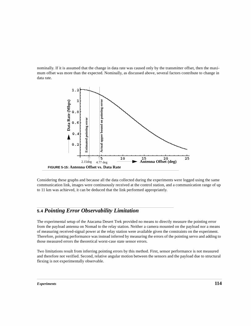
Experiments 114

nominally. If it is assumed that the change in data rate was caused only by the transmitter offset, then the maxi-mum offset was more than the expected. Nominally, as discussed above, several factors contribute to change in data rate.

Considering these graphs and because all the data collected during the experiments were logged using the same communication link, images were continuously received at the control station, and a communication range of up to 11 km was achieved, it can be deduced that the link performed appropriately.

5.4 Pointing Error Observability Limitation

The experimental setup of the Atacama Desert Trek provided no means to directly measure the pointing error from the payload antenna on Nomad to the relay station. Neither a camera mounted on the payload nor a means of measuring received-signal power at the relay station were available given the constraints on the experiment. Therefore, pointing performance was instead inferred by measuring the errors of the pointing servo and adding to those measured errors the theoretical worst-case state sensor errors.

Two limitations result from inferring pointing errors by this method. First, sensor performance is not measured and therefore not verified. Second, relative angular motion between the sensors and the payload due to structural flexing is not experimentally observable.

Antenna Offset (deg)

Dat

a R

ate

(Mbp

s)

2.15deg 4.77 deg

Est

imat

ed p

oint

ing

erro

r

Act

ual u

pper

bou

nd o

n po

inti

ng e

rror

FIGURE 5-15: Antenna Offset vs. Data Rate

115 Experiments

Nonetheless, as mentioned above, the successful functioning of the communications link provides a coarse indication of pointing performance. Furthermore, a key objective of this research, that is, developing and experimentally verifying relationships between various robot system parameters and resulting pointing per-formance measures (i.e. accuracy, power and torque), is met in spite of these limitations. The primary risk due to these limitations is incurred if the results of this research are extrapolated to predict the performance of higher accuracy pointing designs. Even this risk is minimal because, as is discussed later, improving pointing accuracy beyond the objectives set for Nomad would likely be accomplished by employing closed-loop pointing control due to accuracy limitations of available open-loop sensors.

5.5 Experimental Conclusions

Communication was a key to the success of the Atacama Desert Trek and it surpassed the performance expectations. The antenna pointing mechanism performed without failure during the two months of the Ata-cama Desert Trek and enabled communication at ranges of up to 11 km, a record to our knowledge. The suc-cess can be contributed to factors such as appropriate choices of payload, locomotion, state sensors and

mission. The use of a large beamwidth antenna resulted in relaxed ( ) accuracy requirement. An articu-lated chassis with large wheels and large wheel base, combined with slower speed, resulted in smooth robot motion and minimal disturbances to the pointing mechanism. An appropriate choice of sensors limited the predicted cumulative error from the sensors to . The result is a simple pointing mechanism and a suc-cessful open-loop control strategy.

The design was based on a holistic approach and systemic analysis. The experimental results clearly show the effects of different parameters on pointing performance and agree with the simulation results. There were, however, some shortcomings in the experimental method:

• The pointing clearly worked, but with the current experimental setup it was not possible to determine quantitative performance. Closed-loop sensing would enable quantitative measurement of performance. This could be achieved in a variety of ways. For example, pointing errors can be computed by analyzing a video image of the target taken from a camera mounted on the pointing system (possible since target is line-of-sight.) Another method is to use a radio that provides a measurement of signal strength.

• Data rate is the most direct indicator of the communication link performance for this application. How-ever, no clear measurements of the data rate were available. A direct measurement of data rate, probably by computing in real time based on images and telemetry received at the relay station, would give an estimate of the quality of the communication link as well the pointing performance.

This chapter described the experiments performed to evaluate the performance of the communication link and the pointing mechanism. Results were also discussed. Using the systemic approach as discussed in Chapters 3 and 4, tracking exceeded expectations. The next chapter discusses research conclusions.

2.7°

1.55°

Summary and Conclusions 117

CHAPTER 6 Summary and Conclusions

This research investigated the generic problem of tracking from a mobile robot. Tracking is important for many applications including high bandwidth communica-tion by active pointing of high gain antennas and active camera vision. Mobile robot payload tracking requires high slew rates and large articulation ranges in order to sta-bilize and orient a payload while moving over uneven terrain. Both requirements become more demanding as speed and terrain roughness increase. Payload tracking is addressed in other domains, but the solutions from those domains are not directly applicable to the mobile robot payload tracking problem either because power and mass constraints are less stringent (such as for battle tanks and oil rigs), or because slew rate requirements are less severe (such as for satellites and balloons). Mobile robots and especially exploratory robots, however, are usually limited in mass, power and available space, necessitating precision tracking approaches that can meet these additional requirements.

This research considers the complete robot (mechanism, planning and control) to achieve tracking. This systemic approach is important because an independent fine pointing device such as a gimbal alone- without cooperation from locomotion, sus-pension and isolation devices- might not provide the angular excursions and distur-bance rejection needed in rough terrain. As the terrain roughness and corresponding excursions and disturbances increase, so does the need for robot subsystems to func-tionally cooperate to achieve payload tracking.

118 Summary and Conclusions

A tracking strategy based on subsystem interactions was developed along with tools to model and evaluate payload tracking, metrics for evaluating tracking configurations, and guidelines for developing configura-tions suitable for payload tracking from mobile robots.

Communication from mobile robots, especially outdoor mobile robots, is an important capability and was chosen as the application area for this research. A specific challenge is to achieve high data rate communica-tion over an extended range (> 3-4 km) from a robot moving over rough terrain. One method to achieve this is to use an actively pointed high gain antenna. The research configured, designed and demonstrated a mobile robot antenna tracking system capable of tracking a receiver antenna by a robot-mounted transmitter antenna. Tracking design employed a design process, metrics, and analysis tools developed during the research. An antenna pointing device was built and tested. The communication system was successfully demonstrated by achieving high data rate communication from the robot, Nomad, over distances greater than 10 km during the Atacama Desert Trek.

The following sections discuss the contributions, lessons learned and future research directions related to this work.

6.1 Contributions

The main contributions of the work are:

1. Systemic-based payload tracking design

The research developed a systemic-based payload tracking design process. This process optimizes the track-ing solution by evaluating a holistic model of tracking (including the locomotion, pointing device, state sen-sors, planner, control, payload, terrain, and the task). Designs are represented as points in the design space and optimization is achieved by an exhaustive search of this space.This process:

• enables rigorous investigation of the effects of all key system variables to overall tracking performance.

• results in tracking solutions that have advantage (in terms of accuracy, power and weight) over solutions obtained using conventional component-based design approaches.

This process enabled the design and implementation of a simple and successful solution for antenna pointing for Nomad to achieve high bandwidth communication. A seemingly complicated and extremely challenging problem was solved using a simple scheme due to judicious choices of locomotion, pointing device, sensor configuration, payload and mission variables (e.g., speed and range).

Summary and Conclusions 119

2. Payload isolation metrics

In general, greater isolation of payload from terrain disturbances results in a tracking design that is easier to con-trol, and has lower mass and lower power. Vehicle Smoothing Factor (VSF) and coupling together estimate the isolation of the payload due to terrain disturbances. VSF estimates the isolation of the pointing device base from the disturbances caused by traversing terrain, while the coupling estimates the isolation of the payload from dis-turbances incurred at the base of the pointing device.

VSF quantifies the terrain smoothing capability of mobile robots; a higher VSF means that the vehicle provides greater attenuation of terrain disturbances to the pointing device. VSF, as verified in simulation, is inversely pro-portional to the torque and power required for pointing. VSF is important as it:

• can be used to characterize and compare locomotion configurations for tracking tasks and guide optimization searches;

• is the first attempt to characterize low frequency/high amplitude disturbances isolation; and

• captures the relevant functionality (providing smooth motions) of the vehicles for the tracking tasks.

Using this metric, the research quantified the smoothing ability of several wheeled robots and used the metric effectively for screening locomotion configurations during the initial design phase.

Coupling is a measure of disturbances transmission to the pointing payload from disturbances at the base of the pointing device. Kinematic coupling, as developed in this work, gives an estimate of the joint velocities required to maintain an acceptable pointing tolerance. Since this metric is based purely on kinematics of the pointing device, it is relatively easy to calculate. Kinematic coupling is task dependent and hence is suitable for compar-ing pointing devices for a given tracking task. A higher value of kinematic coupling reflects higher torques and the power necessary for tracking, as verified in simulation.

Dynamic coupling, adapted from the work done by Bergerman et al. [13] in regards to underactuated manipula-tors, relates the pointing actuators accelerations, as needed to maintain acceptable pointing, to the disturbance accelerations at the base of the pointing device. The formulation is based on dynamics and hence is a higher fidelity indication of performance (power, torques). As for the case of kinematic coupling, a higher dynamic cou-pling reflects higher torques and the power necessary for tracking.

Global coupling, either kinematic or dynamic, has been defined as the average value of coupling over a represen-tative terrain. This method of calculating coupling is valuable as it is task dependent; hence, it is a useful metric to compare various pointing device options for a given task. It can also be used to characterize pointing devices for tracking tasks and to guide optimization searches.

120 Summary and Conclusions

3. Metrics for sensor configuration

The accuracy of pointing is ultimately limited by the accuracy of the state sensors used. This research devel-oped an analysis technique and proposed two metrics, Sensor Criticality and Senor Configuration Suitabil-ity, to evaluate sensors for tracking tasks. For a given tracking task requirement, the technique evaluates each sensor as well as the sensor configuration as a whole. It is useful for deriving sensor requirements and esti-mating open-loop control error.

Sensor criticalities estimate the appropriateness of each sensor for the task under consideration. Low criti-cality for a sensor means that the output error caused by that particular sensor is small compared to the max-imum allowable error; hence, it indicates whether the given sensor is adequate for the application. Suitability quantifies the appropriateness of a sensor configuration for the task under consideration. Criticality and suit-ability are important metrics as they guide the selection of an adequate sensor configuration. The sensor con-figuration should satisfy the accuracy objectives without incurring unnecessary complexity or cost.

4. Tools to model and evaluate tracking

The research developed a set of analytic and simulation tools to model and evaluate payload tracking perfor-mance of mobile robot configurations. The design process from Chapter 3 is implemented in C-programs, where the inputs are tracking specifications. Several locomotion, pointing and sensor modules are imple-mented in a modular software structure; additional modules can be added easily. These programs can com-pute VSF, as well as kinematic and dynamic coupling; additionally, they can perform the sensitivity analysis for sensors. Mathematica programs were developed to compute the dynamics based on the input forward kinematics. The dynamics can be directly imported in a C-program where the chosen designs can be fine-tuned along with controller design and implementation.

These programs allow rapid generation and evaluation of tracking designs for mobile robot applications.

5. A successful tracking design development and demonstration

The research configured, designed and demonstrated a mobile robot antenna tracking system capable of tracking a receiver antenna by a robot-mounted transmitter antenna. Tracking design used the design process and tools developed during the research. Tracking was demonstrated during the course of the 200 km, 2 month experiment with the vehicle traversing diverse terrains of the Atacama desert at speeds of up to 40 cm/s, and at varying ranges and orientations with respect to the target. During the test, the vehicle distur-

bance rates (roll/pitch/yaw rates) were up to .This demonstrated:

• low power tracking from a mobile robot traversing natural terrain, and

• high data rate communication over extended ranges from outdoor mobile robots for the first time. This technology is key to planetary exploration by robots.

25° s⁄

Summary and Conclusions 121

6.2 Lessons Learned

• Closed-loop sensing is desirable: Controller error was quite small as compared to the error due to sensors even for a simple PID controller. The estimated cumulative error due to the sensors was approximately

. The sensors used on Nomad were among the best available and so alternate sensors in the same con-figuration may be inadequate for higher precision applications. Sensor fusion should enable somewhat better accuracies. A better strategy, however, is to implement closed-loop sensing, e.g. by using a camera to sight the target which is visible due to line-of-sight communication restriction, or by using a signal strength mea-surement. Closed-loop sensing is key to the higher precision applications.

• Include risk mitigation in initial planning: The Atacama Desert Trek was a fast track project with a design cycle of less than a year. The pointing system, being the product of this research, was experimental, and thus pointing performance could not be guaranteed a priori. Therefore, because the communication function was required for the other objectives of the Atacama Desert Trek, contingencies were planned. If the pointing per-

formance was not achieved for the beamwidth antenna (having a maximum allowable offset- ), an

beamwidth antenna (with a maximum allowable offset- ) could be used at the expense of reduced communication range. If pointing performance was unable to meet the requirements for this second antenna, a third antenna, with a beamwidth, would have been used with a further reduction in the range. In the worst case (pointing mechanism failure), an omnidirectional antenna would have been used (range ~ 1 km). Thus, alternates assured a path to success.

• Phased arrays are not yet ready: Phased array antennas were considered for the communication system because they enable electronic pointing. Although the technology continues to advance, it is still is not ready for use in this class of mobile robots due to higher cost and mass in comparison to mechanical pointing con-trol.

• RF rotary joints proved effective: An RF rotary joint worked well for this application. RF rotary joints do not impose the high losses of flexible RF which would effectively negate the gain advantage provided by a high gain antenna. Hence, flexible RF cables should be avoided for these applications.

6.3 Research Directions

Locomotion: Active control of locomotion has interesting implications for tracking performance. In general, controllable suspensions (active or semi-active suspension) have better terrain smoothing capabilities than pas-sive suspensions and could be advantageous for tracking tasks, but at the cost of added complexity. Complexity in locomotion can be traded for complexity in the pointing device.

Planner: It would be useful to implement another hazard module in Morphin that considers tracking needs. Speeds, obstacle sizes and turning radius could be actively changed to either improve pointing performance or reduce the mass and power of the pointing system.

1.55°

27° 2.7°80° 8.0°

180°

122 Summary and Conclusions

Coupling: The coupling metrics developed were not fully exploited in the thesis. Coupling could also be used for minimal power trajectory generation for the pointing actuators. Since global coupling is state dependent, it is possible to choose trajectories such that the coupling, and hence power, is minimized. If the payload has to be moved from A (Az1, El1) to B(Az2, El2), a trajectory based on coupling metric can be generated such that the power required for pointing is minimized. Also, since the dynamic coupling depends on the geometric and inertia parameters, it can be used for the optimal placement on the pointing device as well as the design of the pointing device [73].

A coupling metric could also be developed for energy. For example, in the formulation of kinematic cou-pling, if each of the speeds is multiplied by the inertia tensors at the outset, a similar derivation procedure could lead to a metric that minimizes energy instead of the sum of the actuator speeds.

Closed-loop pointing error feedback: As discussed above, the pointing accuracy was limited because pointing was accomplished using open-loop sensing. The key to further improve pointing performance is to implement closed-loop pointing error feedback. Improved pointing accuracies would allow the use of higher gain antennas for extended range. Also, appreciable literature exists on the end pointing control of manipula-tors, which could be extended to the tracking control problem once closed-loop sensing is available.

Robot-satellite communication: Direct satellite communication, an extension of the problem, is relevant to planetary missions where a robot could directly communicate with the Earth and would not need to be in the vicinity of a lander-based relay station or within view of an orbiting relay station. In Atacama Desert Trek-like scenarios, it would completely eliminate the local relay station, thus greatly simplifying total system complexity and logistics. The challenge is to align a larger, higher gain, narrower beamwidth antenna, neces-

sary due to increased range, with far better accuracy (~ ).

An alternate approach to pointing a dish mechanically is to use a phased array antenna. Phased array anten-nas have the following advantages over conventional dish antennas: electronic pointing, conformal surfaces, no moving parts, and slightly better efficiencies. Also by virtue of the design, it is easier to implement signal strength measurement in a phased array. Although the phased arrays are not cost effective at this time, within a few years they might be common. These could revolutionize high bandwidth communication for mobile applications.

This research investigated the generic problem of tracking from a mobile robot. A tracking strategy based on subsystem interactions was developed along with tools to model and evaluate payload tracking, metrics for evaluating tracking configurations, and guidelines for developing configurations suitable for payload track-ing from mobile robots. The strategy was implemented to design a communication system to achieve high bandwidth communication from a desert exploring mobile robot using active pointed high gain antennas. This was demonstrated during the course of the 200 km, two month experiment with the vehicle traversing diverse terrains of the Atacama desert, at speeds up to 40 cm/s, and at varying ranges and orientations with respect to the target. The antenna pointing mechanism performed without failure and enabled communica-tion at ranges of up to 11 km, to our knowledge, a record for this class of machines. This work, although lim-ited in scope, is hopefully an important step towards designing tracking systems for mobile robot applications.

0.2°

123

Appendix A Dynamic Model

Simulations were performed to estimate the effects of coupling and to evaluate vari-ous control algorithms. To simplify the analysis, the robot was assumed to be moving in a plane (Figure A-1). To point anywhere in the world, two axes (azimuth and eleva-tion) are required.

The equations governing dynamics of the mechanism were obtained using the formu-lation given in [42]. The dynamics can be represented as:

FIGURE A-1: Simplified Model for Simulation

Robot

Z

Y

γ Relay Station

Antenna Pointing Mechanism (2 dof)

Mq·· V q· q,( )q· G+ + τ=

124

where is the generalized position vector, is a inertia matrix, is a

matrix s.t. gives the centripetal and coriolis forces, is a matrix of gravity terms, and is vector of generalized forces. Here,

Y-coordinate of the vehicle in the inertial frame

Z-coordinate of the vehicle in the inertial frame

Pitch of the vehicle

Azimuth of the pointing device

Elevation of the pointing device

The complete system is 5 dof, but only two ( and ) of these of these are controllable. These correspond

to the last two rows of the matrices in the above equation. After rearranging we get the following equation corresponding to two controllable dofs,

where,

, , ,

, , , and .

The terms of these matrices are defined below.

Mass Matrix

q yv zv γ αp γp, , , ,[ ]= M 5 5× V 5 5×

Vq· G 5 1× τ 5 1×

yv

zv

γ

αp

γp

αp γp

Mq··

Vq·

G+ + τ Mbq··

– Vbq·

–=

Mm44 m45

m54 m55

= Vv44 v45

v54 v55

= GG4

G5

=

ττ4

τ5= Mb

m41 m42 m43

m51 m52 m53= Vc

v41 v42 v43

v51 v52 v53= q q4 q5,[ ]

T= qb q1 q2 q3, ,[ ]

T=

m41 γ a42– e42 γpcos– e43 γpsin+( ) αp a41 e41+( ) αpcos+sin[ ]cos=

125

Coriolis and Centripetal Terms

m42 γsin a42– e42 γpcos– e43 γpsin+( ) αp a41 e41+( ) αpcos+sin[ ]=

m43 αp a31– zp a41 e41+( )– e31 γpcos– e21 γpsin–{ } αp a32 zp a42 e42 γpcos e43 γpsin+ +( )e23 2γpcos 0.5e22 e33–( ) 2γpsin

+

+ +

{}

sin+cos=

m44 a11 a22 e11 0.5 1 2γpcos+( )e22 e23 2γpsin– 0.5 1 2γpcos–( )e33+ + + +=

m45 e13 γpcos– e12 γpsin–=

m51 e42 γpsin e43 γpcos+( ) αpcos γ e43 γpsin e42– γpcos( ) γsin+cos–=

m52 e42 γpsin e43 γpcos+( ) αpcos γ e43 γpsin e42– γpcos( )– γcossin–=

m53 zp e42 γpsin e43 γpcos+( ) αpcos e22 e33+( ) αp e12 γpcos e13 γpsin–( ) αpyp– e43 γpsin e42– γpcos( )

sin+cos+=

m54 m45=

m55 e22 e33+=

v41 0=

v42 0=

ν43 yp αp e24 γp e34 γpsin–cos a24+( ) 0.5 a12 e12 γpcos e13 γpsin–+( ) 2αp yp– αp a14 e14+( )

0.5 2αp a11– a22 e11– e22 γpcos( )2

e33 γpsin( )2

2e23 2γpsin–+ + + sin+

coscos–sin

q3·

αp e22 γpcos( )2

e33 γpsin( )2

e23 2γpsin–+ αp e13 γpsin e12 γpcos–( )cos+sin q5

·+

=

126

Gravity Terms

In the above equations, and are the terms of inertia tensors for azimuth and elevation assem-

blies respectively.

v44 e23– 2γpcos 0.5 2γp e33 e22–( )sin+[ ]q·5=

v45 αp e22 γpcos( )2

e33 γpsin( )2

e23 2γpsin–+ αp e13 γpsin e12 γpcos–( )cos+sin q·3

e23– 2γpcos 0.5 2γp e33 e22–( )sin+[ ]q·4 e12 γpcos– e13 γpsin+[ ]q·5+ +

=

v51 0=

v52 0=

v53 αpsin–( )2

e23 2γpcos 0.5 2γp e22 e33–( )sin+{ } yp αp e34 γpcos e24 γpsin+( )

zp e34 γpsin e24 γpcos–( ) 0.5 2αp e13 γpcos e12 γpsin+( )sin+ +

cos+

q·3

αp e– 22 γpcos( )2

e33– γpsin( )2

e23 2γpsin+ αp e13 γpsin e12 γpcos–( )cos–sin q·4+

=

v54 αp e– 22 γpcos( )2

e33– γpsin( )2

e23 2γpsin+ αp e13 γpsin e12 γpcos–( )cos–sin q·3

e23 2γpcos 0.5e22 e33–( ) 2γpsin+[ ]q·4+

=

v55 0=

G4 g γ αp a24 e24 γpcos e34– γpsin+( ) a14 e14+( ) αpcos+sin–[ ]sin=

G5 g αpcos γ e24– γpsin e34 γpcos–( ) γ e24 γpcos e34 γpsin–( )cos+sin[ ]=

aij eij 4 4×

127

APPENDIX B References

[1] J. Aloimonos and D.P. Tsakiris, “On the Mathematics of Visual Tracking”, Computer Science Technical Report Series, University of Maryland, College Park. CAR-TR-390, CS-TR-2102, September 1988.

[2] W.W. Anderson, N.J. Groom and C.T. Woolley, “The Annular Suspension and Pointing System”, Automatic Control in Space, Proceedings of the 8th IFAC Symposium, Oxford, England, 2-6 July 1979 Editor C.W. Munday, pp 41-49.

[3] J. Andrus and E. Korzeniowski”, Modular Antenna Pointing System for the Explorer Platform Satellite”, 26th Aerospace Mechanisms Symposium, Green-belt, Maryland, May 13-15, 1992, pp 111-126.

[4] M. Bachmann, J.H. Decanini, and J.G. Zaremba, “Development and Testing of a Precision Pointer/Tracker for a Spinning aircraft”, Guidance and Control 1985, Vol 57. Proceedings of the Annual Rocky Mountain Guidance and Con-trol Conference, Feb 2-6, 1985, Keystone, CO. Edited by Robert D. Culp, Edward J. Bauman, Charles A. Cullian, pp89-118.

[5] D. Bapna, E. Rollins, J. Murphy, M. Maimone, W. Whittaker, and D. Wettergreen, “The Atacama Desert Trek: Outcomes”, Proceedings of the1998 IEEE International Confer-ence on Robotics and Automation, Leuven, Belgium, May 16-20, 1998.

[6] D. Bapna, E. Rollins, A. Foessel, and W. Whittaker, “Antenna Pointing for High Band-width Communications from Mobile Robots”, Proceedings of the1998 IEEE Interna-tional Conference on Robotics and Automation, Leuven, Belgium, May 16-20, 1998.

128

[7] D. Bapna, J.P. Teza, E. Rollins, and W. Whittaker, “An Innovative High Bandwidth Communication System for Mobile Robots”, 27th International Conference on Environmental Systems, Lake Tahoe, Nevada, July 14-17, 1997, SAE Technical Series, Paper 972488.

[8] D. Bapna, W. Whittaker and N. Colella, “Direct Communication from a Lunar Rover to Earth Enabled by Precision Pointing”, International Lunar Exploration Conference, San Diego, Nov, 1994.

[9] David Baraff, “SIMKITTM User Reference Manual”, Internal document, Carnegie Mellon University. SIMKITTM was developed at CMU by Dr. David Baraff.

[10] J. E. Bares and W. L. Whittaker, “Configuration of Autonomous Walkers for Extreme Terrain”, The International Journal of Robotics Research, Vol. 12, No. 6, December 1993, pp. 535-559.

[11] K.E. Barker, “A Simple Demonstration of Laser Beam Stabilization”, Guidance and Control 1988, Advances in the Astronautical Sciences, Volume 66, pp203-210.

[12] M.G. Bekker, “Introduction to Terrain-Vehicle Systems”, The University of Michigan Press, Ann Arbor, 1969.

[13] M. Bergerman, C. Lee and Y. Xu, “Dynamic Coupling of Underactuated Manipulators”, Proceedings of the 4th IEEE Conference on Control Applications, Albany, USA, Sept. 1995, pp. 500-505.

[14] A.J. Besonis and C.J. Chang, “Evaluation of Communication Antenna Drive System Requirements to Allow TDRS Tracking During LST Fine Pointing”, Space Shuttle Missions of the 80's, Advances in the Astronautical Sciences, Volume 32, Part 1, pp413-417.

[15] B. Brown, “Gyroscopic Stabilization”, Personal Communication, The Robotics Institute, Carnegie Mellon University, Pittsburgh, PA 15213.

[16] C.P. Chaloner, M.E. Farman and A.L. Hardie, “A Balloon-Borne Three Axis Stabilized Platform for Large Astronomy Experiments”, Automatic Control in Space, Proceedings of the 8th IFAC Sympo-sium, Oxford, England, 2-6 July 1979, Editor C.W. Munday, pp 9-17.

[17] J. E. Chottiner, “Simulation of a Six Wheeled Martian Rover called a Rocker Bogie”, Masters thesis, Department of Mechanical Engineering, The Ohio State University, 1992.

[18] E.G. Cowart, “Lunar Roving Vehicle: Spacecraft on wheels”, The Institution of Mechanical Engineers, Proceedings 1973, Volume 187 45/73, pp463-491.

[19] X. Cui and K.G. Shin, “Robot Trajectory Tracking With Self-Tuning Predicted Control”, Center for Research on Integrated Manufacturing, The University of Michigan, Ann Arbor, Michigan, RSD-TR-13-87, August 1987.

[20] N.D. Dang, B. Claydon and P. Crilley, “A Stabilized Satellite Terminal for Hostile Marine Environ-ments”. Source Unknown.

[21] R.B. Deadrick, “Design and Performance of a Satellite Laser Communication Pointing System”, Guid-ance and Control 1985, Vol 57. Proceedings of the Annual Rocky Mountain Guidance and Control Conference, Feb 2-6, 1985, Keystone, CO. Edited by Robert D. Culp, Edward J. Bauman, Charles A. Cullian, pp155-166.

[22] J. R. Ellis, “Vehicle Dynamics”, Business Books, London, 1969.

129

[23] J. Emura et. al., “Development of the Semi-Active Suspension System Based on the Sky-Hook Damper Theory”, Vehicle Suspension System Advancements, SP-1031, Published by Society of Automotive Engi-neers, Inc., February 1994, pp17-26.

[24] R.L. Gates, H.H. Wine, R.W. Seiferth, and N.A. Osborne, “Development of a Large-Inertia Fine-Pointing and Dimensional Stability Simulator”, Space Shuttle Missions of the 80's, Advances in the Astronautical Sciences, Volume 32, Part 1, pp409-412.

[25] T.D. Gillespie, “Fundamentals of Vehicle Dynamics”, Society of Automotive Engineers, Inc., Warrendale, PA, U.S.A., 1992.

[26] A.A. Gupta and L.M. Germann, “Precision Pointing and Inertial Line-of-sight Stabilization Using Fine-Steering Mirror, and Strap-Down Inertial Sensors”, Guidance and Control 1989, Advances in the Astro-nautical Sciences, Volume 68, pp325-336.

[27] S. Hanagud, S. Sarkar, G.L. NageshBabu and E.K. Hall, “Adaptive Sensors and Actuators in the Vibration Control of Rotating and Pointing Systems”, Second Joint Japan/U.S. Conference on Adaptive Structures, November 12-14 1991, Nagoya, Japan. Edited by Y. Matsuzaki and B.K. Wada, pp164-183.

[28] C.W. Henrikson and E.E. Schmidt, “A Small Instrument Pointing System For Shuttle Sortie Missions”, Space Shuttle Missions of the 80's, Advances in the Astronautical Sciences, Volume 32, Part 1, pp418-421.

[29] M. Herald and L. C. Wai, “Two-Axis Antenna Pointing Mechanism”, 28th Aerospace Mechanisms Sympo-sium, Cleveland, Ohio, May 18-20, 1994, pp 183-197.

[30] H. Heusmann and J.C. Jones, “A Fine-Pointing Facility for Spacelab Experiments in the 1980's- The Instrument Pointing Subsystem”, Space Shuttle Missions of the 80's, Advances in the Astronautical Sci-ences, Volume 32, Part 1, pp422-425.

[31] C.O. Highman, “A Scanning Mirror System for the Apollo Telescope Mount Ultraviolet Spectroheliome-ter”, 5th Aerospace Mechanisms Symposium, Greenbelt, Maryland, June 15-16, 1970, pp 113-120.

[32] S. Hirose and N. Ootsukasa, “Design and Development of a Quadra-Rhomb Rover for Mars Exploration”, ICAR 1993, pp109-112.

[33] I.C. Holm, “Articulated, Wheeled Off-the-Road Vehicles”, Journal of Terramechanics, 1970, volume 7, No. 1, pp19-54, Pergamon Press, Great Britain.

[34] G. Hyde, ed. “NASA/NSF Panel Report on- Satellite Communications Systems and Technology”, Interna-tional Technology Research Institute, JTEC/WTEC Program, Loyala College in Maryland, July, 1993.

[35] G. R. Jessop. “VHF/UHF Manual”, Fourth Edition, Radio Society of Great Britain. Garden City Press Ltd., Letchworth, Hertfordshire, 1983.

[36] L. Katragadda, J. Murphy and W. Whittaker, “Rover Configuration for Entertainment-based Lunar Excur-sion”, International Lunar Exploration Conference, San Diego, Nov, 1994.

[37] A. J. Kelly, “An Intelligent Predictive Controller for Autonomous Vehicles”, CMU Robotics Institute Tech-nical Report CMU-RI-TR-94-20.

[38] A. Kemurdjian, et. al., “Small Marsokhod Configuration”, Proceedings of the 1992 IEEE International Conference on Robotics and Automation, Nice, France- May 1992, pp165-168.

130

[39] T. Kitsuregawa. “Advanced technology in satellite communication antennas: electrical and mechanical design”. Artech House, Norwood, Mass., 1990.

[40] P.R. Klarer and J.W. Purvis, “A Highly Agile Chassis Design for a Robotic All-Terrain Lunar Explora-tion Rover”, American Nuclear Society Conference, Knoxville TN, 1993.

[41] W. J. Larson and J. R. Wertz. “Space Mission Analysis and Design”, second Edition, Kluwer Aca-demic Publishers, 1992.

[42] F.L. Lewis, C.T. Abdallah, and D.M. Dawson, “Control of Robot Manipulators”, Macmillan Publish-ing Company, New York, 1993.

[43] D. Lukaszewski and N. Osborne, “Payload Isolation for Fine Pointing”, Aerospace Century XXI: Space Flight Technologies, Advances in the Astronautical Sciences, Volume 64, Part II, pp 747-763, Proceedings of the 33rd Annual AAS International Conference held October 26-29, 1986, Boulder, CO.

[44] R.A. Lindemann and H.J. Eisen, “Mobility Analysis, Simulation and Scale Model Testing for the Design of Wheeled Planetary Rovers”, Proceedings of the Conference on Missions, Technology and Design of Planetary Mobile Vehicles, Toulouse, France, 1992, pp. 531-536.

[45] M. F. Luniewicz, J.P. Gilmore, Tze Thong Chein, J. E. Negro and Captain R. L. Wingler, “Comparison of Wide-band inertial Line of Sight Stabilization Reference Mechanizations”, Presented at SPIE Aero-space Sensing, Acquisition, Tracking and Pointing VI, Orlando, Florida, April 21-24, 1992.

[46] R. Malueg, N.J. Colella and D. Hakala “Stabilized Optical Tracking Platform for Airborne Applica-tions” Personal Communication.

[47] D. Manko, “A General Model of Legged Locomotion on Natural terrain”, Ph.D. thesis, Department of Civil Engineering, Carnegie Mellon University, 1990.

[48] J.R. Mitchell, H.E. Worley and S.M. Seltzer, “Digital Control System Design for a Precision Pointing System”, Guidance and Control 1983, Advances in the Astronautical Sciences, Volume 51, pp39-51.

[49] D. Moline et. al., “Simulation and Evaluation of Semi-Active Suspensions”, Vehicle Suspension Sys-tem Advancements, SP-1031, Published by Society of Automotive Engineers, Inc., February 1994, pp27-37.

[50] W. L. Morgan and G. D. Gordon. “Communications Satellite Handbook”, John Wiley & Sons, New York, 1989.

[51] J. Murphy, “Application of Panospheric Imaging to a Teleoperated Lunar Rover,” IEEE Intl. Conf on Systems, Man and Cybernetics. 1995. Vol 4.

[52] K.S. Narendra and A.M. Annaswamy, “Stable Adaptive Systems”, Prentics Hall Inc., Englewood Cliffs, N.J., U.S.A, 1989.

[53] K. Ogatta, “Modern Control Engineering”, Second Edition, Prentice-Hall, Inc., Englewood Cliffs, N.J., U.S.A, 1992.

[54] Orbit Advanced Technologies, 905 Sheehy Drive, Bldg. G, Babylon Business Campus, Horsham, PA 19044, USA.

131

[55] M.A. Ostaszewski and L.J. Guy, “Pointing/Roll Mechanism for the Ultraviolet Coronagraph Spectrome-ter”, 25th Aerospace Mechanisms Symposium, Pasadena, California, May 8-10, 1991, pp93-105.

[56] S.J. Paddack, “Pointing Requirements for Space Station Science”, Guidance and Control 1983, Advances in the Astronautical Sciences, Volume 51, pp247-256.

[57] C.D. Padula, et. al., Automatic Control in Space, Proceedings of the 8th IFAC Symposium, Oxford, England, 2-6 July 1979,Editor C.W. Munday, pp 19-23.

[58] M. Pelizzari and D. Driswell. Lunar dust transport by photoelectric charging at sunset. Proc. of the Lunar Planetary Science Conference. 1978

[59] Linda S. Robeck, David B. Rathbun, and David H. Lehman. “Precision Pointing for an Orbital Earth Observing System”. Presented at the 1990 American Control Conference, San Diego, CA, May 23-25, 1990.

[60] F. Schmitt, “Mechanisms of the Space Active Vibration Isolation (SAVI)”, 26th Aerospace Mechanisms Symposium, Greenbelt, Maryland, May 13-15 1992, pp245-262.

[61] J.T. Sears and V.T. Durnell, “Cost-Effective Two-Axis Pointing Gimbal”, Guidance and Control 1983, Advances in the Astronautical Sciences, Volume 51, pp129-134.

[62] S. W. Sirlin and R.A. Laskin, “Payload Isolation and Precision Pointing for the 1990", Guidance and Con-trol 1985, Vol 57. Proceedings of the Annual Rocky Mountain Guidance and Control Conference, Feb 2-6, 1985, Keystone, CO. Edited by Robert D. Culp, Edward J. Bauman, Charles A. Cullian, pp39-60.

[63] R. Simmons, L. Henriksen, L. Chrisman, and G. Whelan, “Obstacle Avoidance and Safeguarding for a Lunar Rover”, Proc. AIAA Forum on Advanced Developments in Space Robotics, Aug. 1996, Madison, WI.

[64] N. Takada, T. Amano, T. Ohhashi and S. Wachi, “An Antenna-Pointing Mechanism for the ETS-VI K-Band Single Access (KSA) Antenna”, 25th Aerospace Mechanisms Symposium, Pasadena, California, May 8-10, 1991, pp77-92.

[65] K. Tani, et. al., “Active Suspension Four-Wheel Model for a Terrain Robot”, IEEE/RSJ International Workshop on Intelligent Robots and Systems (IROS), Tsukuba, Japan, pp. 408-413, September 4-6, 1989.

[66] D. Wettergreen, H. Pangels and J. Bares, “Behavior-based Gait Execution for the Dante II Walking Robot”, Proc. IEEE/RSJ conf. on Intelligent Robots and Systems, Vol. 3, August 1995, pp. 274-279.

[67] W. Whittaker, D. Bapna, M. Maimone, and E. Rollins, “Atacama Desert Trek: A Planetary Analog Field Experiment”, Proceedings of i-SAIRAS 97, Tokyo, Japan, July 14-16, 1997, pp355-360.

[68] W. Whittaker et al. “JTEC Panel Report on Space Robotics in Japan”, Japanese technology Evaluation Center, Coordinated by Loyala College in Maryland, 1991.

[69] W. Whittaker et al.,”Entertainment Based Lunar Rover Mission Concept”, Technical Report, Lunar Rover Initiative, CMU, Pittsburgh, PA, December 1994.

[70] P. Wiktor, “A Reactionless Precision Pointing Actuator”, 21st Aerospace Mechanisms Symposium, Hous-ton, Texas, April 29-May1 1987, pp 165- 174.

132

[71] B. Wilcox, et. al., “Robotic Vehicles for Planetary Exploration”, Proceedings of the 1992 IEEE Inter-national Conference on Robotics and Automation, Nice, France- May 1992, pp175-180.

[72] J.I. Woodfill, “Motion Vision and Tracking for Robots in Dynamic, Unstructured Environments”, Ph.D. thesis, Department of Computer Science, Stanford University, Stanford, CA, Report No. STAN-CS-92-1440, August 1992.

[73] Y. Xu, “The Measure of Dynamic Coupling of Space Robot Systems”, Proceedings of the IEEE Inter-national Conference on Robotics and Automation, Atlanta, GA, May 1993.

[74] http://kvh home page