Maria-Florina Balcan

04/08/2015

PCA, Kernel PCA, ICA

Learning Representations.

Dimensionality Reduction.

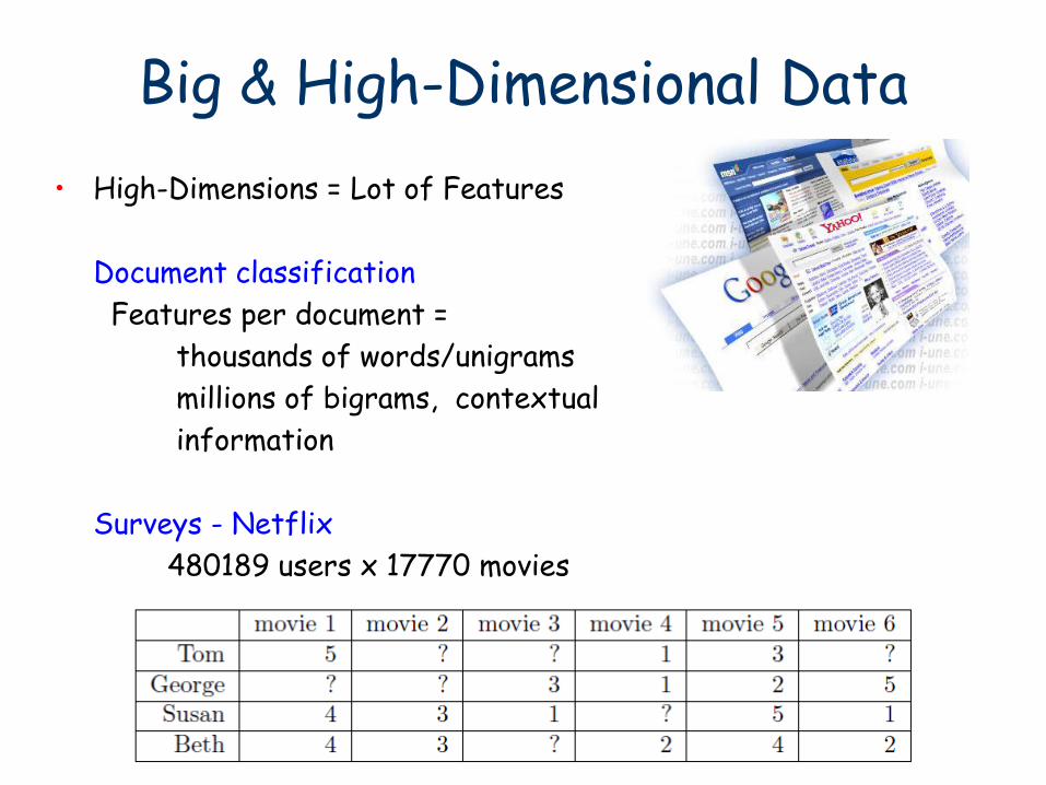
• High-Dimensions = Lot of Features

Document classification

Features per document =

thousands of words/unigrams

millions of bigrams, contextual

information

Surveys - Netflix

480189 users x 17770 movies

Big & High-Dimensional Data

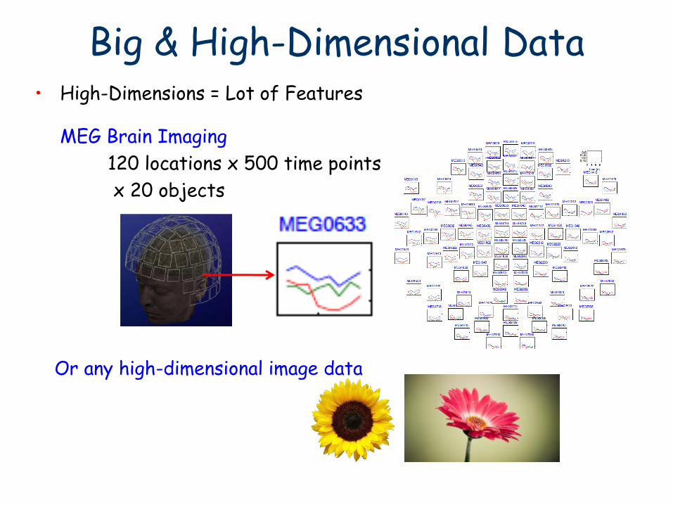
• High-Dimensions = Lot of Features

MEG Brain Imaging

120 locations x 500 time points

x 20 objects

Big & High-Dimensional Data

Or any high-dimensional image data

• Useful to learn lower dimensional representations of the data.

• Big & High-Dimensional Data.

PCA, Kernel PCA, ICA: Powerful unsupervised learning techniques for extracting hidden (potentially lower dimensional) structure from high dimensional datasets.

Learning Representations

Useful for:

• Visualization

• Further processing by machine learning algorithms

• More efficient use of resources (e.g., time, memory, communication)

• Statistical: fewer dimensions better generalization

• Noise removal (improving data quality)

Principal Component Analysis (PCA)

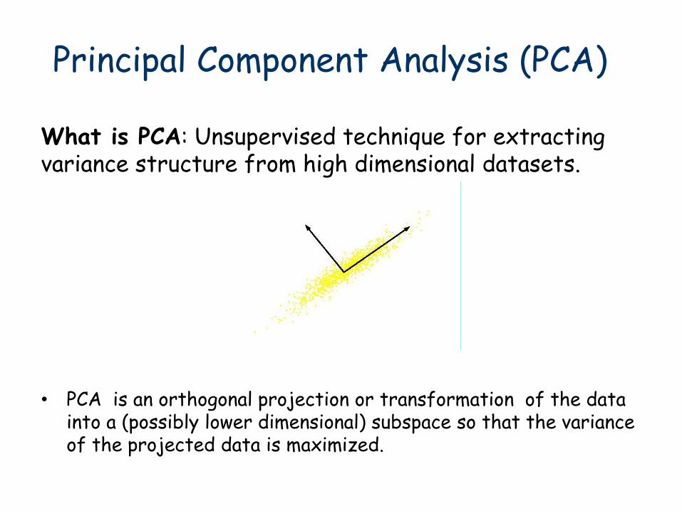
What is PCA: Unsupervised technique for extracting variance structure from high dimensional datasets.

• PCA is an orthogonal projection or transformation of the data into a (possibly lower dimensional) subspace so that the variance of the projected data is maximized.

Principal Component Analysis (PCA)

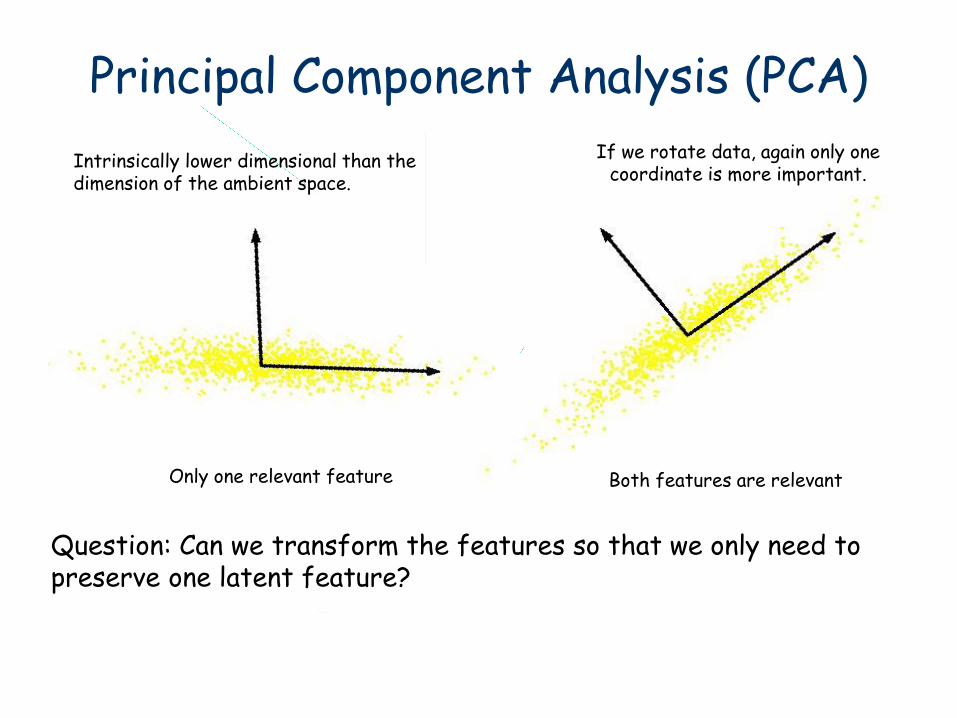
Both features are relevant Only one relevant feature

Question: Can we transform the features so that we only need to preserve one latent feature?

Intrinsically lower dimensional than the dimension of the ambient space.

If we rotate data, again only one coordinate is more important.

Principal Component Analysis (PCA)

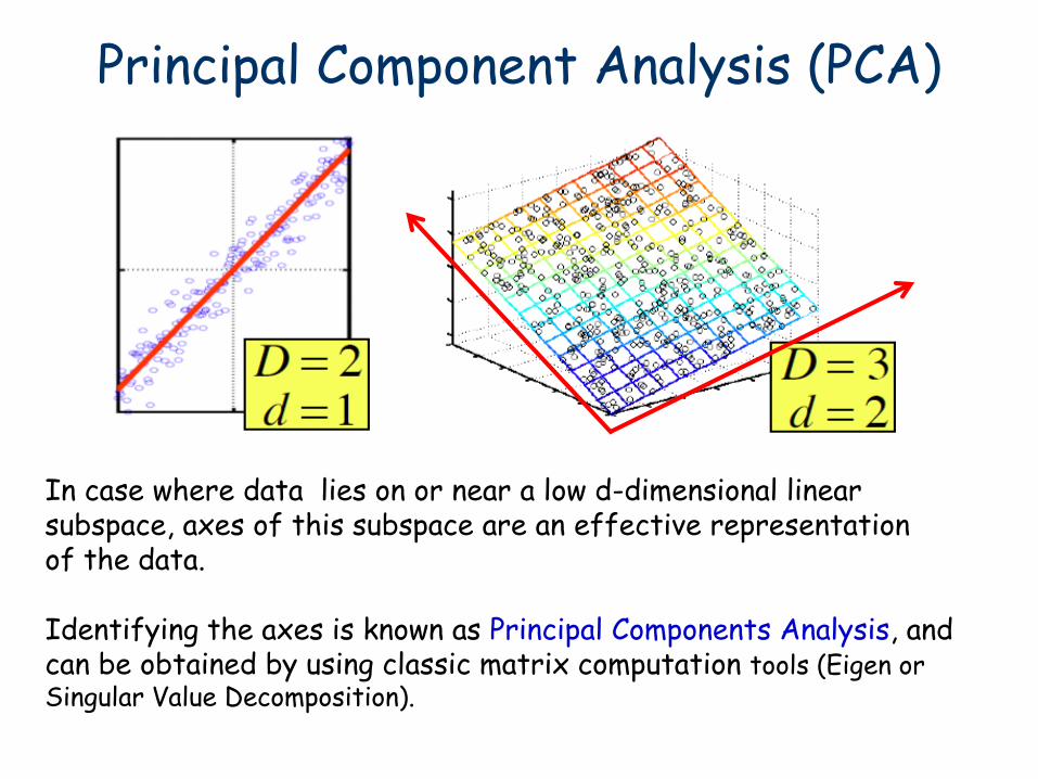
In case where data lies on or near a low d-dimensional linear subspace, axes of this subspace are an effective representation of the data.

Identifying the axes is known as Principal Components Analysis, and can be obtained by using classic matrix computation tools (Eigen or Singular Value Decomposition).

Principal Component Analysis (PCA)

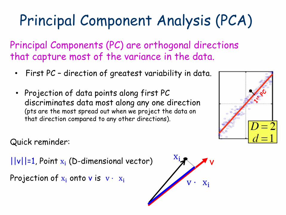
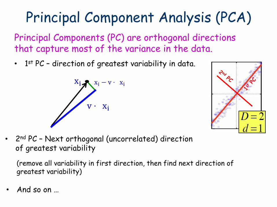
Principal Components (PC) are orthogonal directions that capture most of the variance in the data.

xi v

v ⋅ xi

• Projection of data points along first PC discriminates data most along any one direction (pts are the most spread out when we project the data on that direction compared to any other directions).

||v||=1, Point xi (D-dimensional vector)

Projection of xi onto v is v ⋅ xi

• First PC – direction of greatest variability in data.

Quick reminder:

Principal Component Analysis (PCA) Principal Components (PC) are orthogonal directions that capture most of the variance in the data.

xi − v ⋅ xi xi

v ⋅ xi

• 1st PC – direction of greatest variability in data.

• 2nd PC – Next orthogonal (uncorrelated) direction of greatest variability

(remove all variability in first direction, then find next direction of greatest variability)

• And so on …

Principal Component Analysis (PCA)

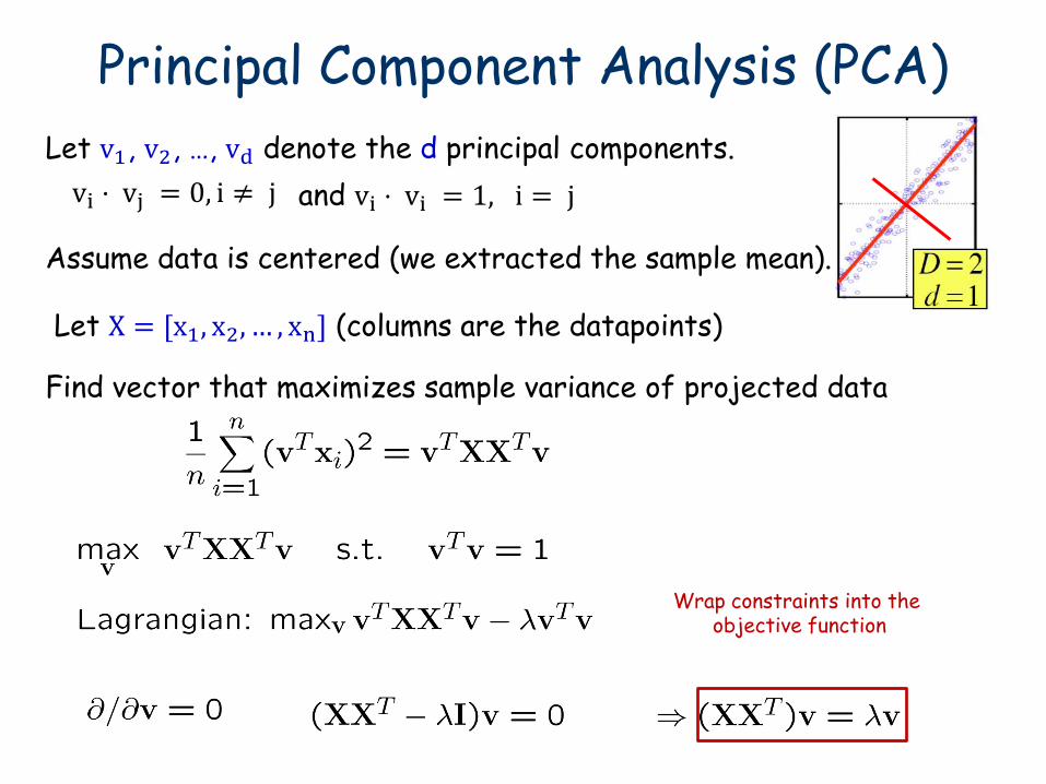
Let v1, v2, …, vd denote the d principal components.

Wrap constraints into the objective function

vi ⋅ vj = 0, i ≠ j

Find vector that maximizes sample variance of projected data

and vi ⋅ vi = 1, i = j

Let X = [x1, x2, … , xn] (columns are the datapoints)

Assume data is centered (we extracted the sample mean).

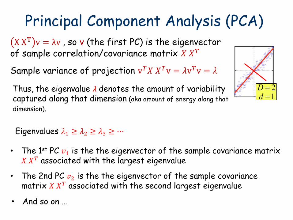
Principal Component Analysis (PCA) X XT v = λv , so v (the first PC) is the eigenvector

of sample correlation/covariance matrix 𝑋 𝑋𝑇

Sample variance of projection v𝑇𝑋 𝑋𝑇v = 𝜆v𝑇v = 𝜆

Thus, the eigenvalue 𝜆 denotes the amount of variability captured along that dimension (aka amount of energy along that

dimension).

Eigenvalues 𝜆1 ≥ 𝜆2 ≥ 𝜆3 ≥ ⋯

• The 1st PC 𝑣1 is the the eigenvector of the sample covariance matrix 𝑋 𝑋𝑇 associated with the largest eigenvalue

• The 2nd PC 𝑣2 is the the eigenvector of the sample covariance matrix 𝑋 𝑋𝑇 associated with the second largest eigenvalue

• And so on …

x1

x2

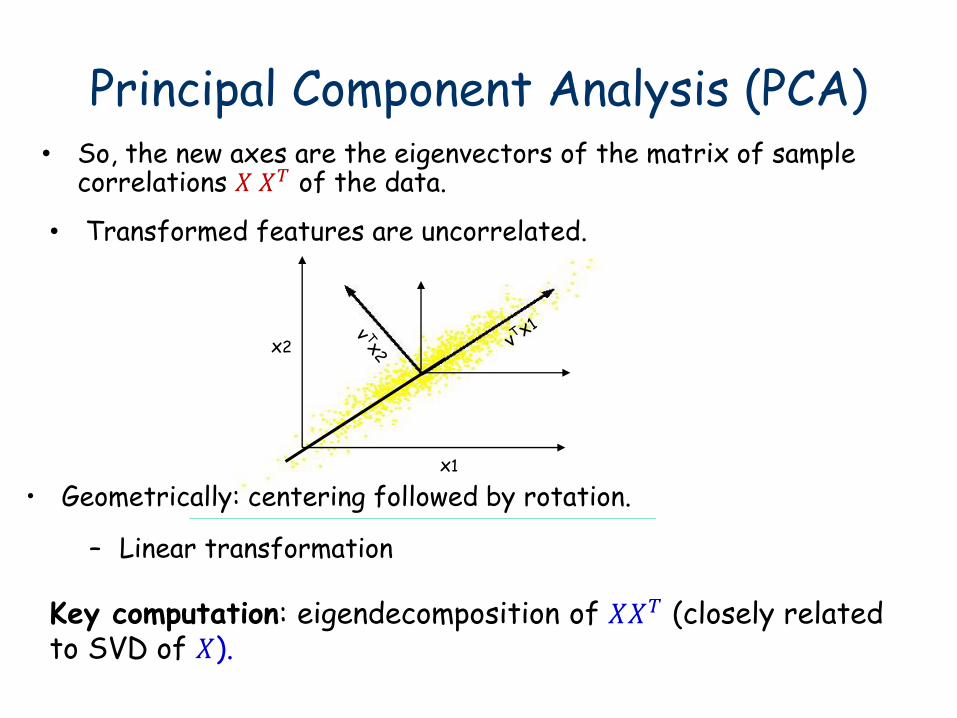
• Transformed features are uncorrelated.

• So, the new axes are the eigenvectors of the matrix of sample correlations 𝑋 𝑋𝑇 of the data.

• Geometrically: centering followed by rotation.

Principal Component Analysis (PCA)

– Linear transformation

Key computation: eigendecomposition of 𝑋𝑋𝑇 (closely related to SVD of 𝑋).

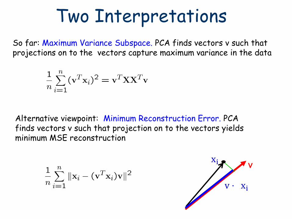
Two Interpretations So far: Maximum Variance Subspace. PCA finds vectors v such that projections on to the vectors capture maximum variance in the data

Alternative viewpoint: Minimum Reconstruction Error. PCA finds vectors v such that projection on to the vectors yields minimum MSE reconstruction

xi v

v ⋅ xi

Two Interpretations

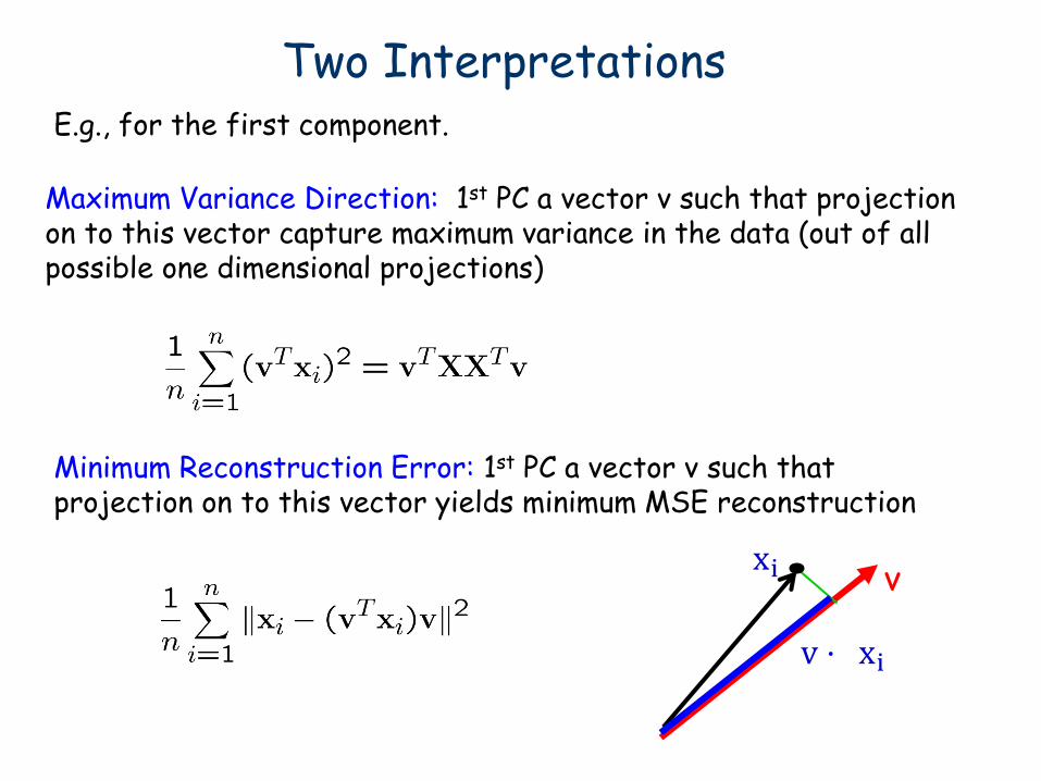
Maximum Variance Direction: 1st PC a vector v such that projection on to this vector capture maximum variance in the data (out of all possible one dimensional projections)

Minimum Reconstruction Error: 1st PC a vector v such that projection on to this vector yields minimum MSE reconstruction

xi v

v ⋅ xi

E.g., for the first component.

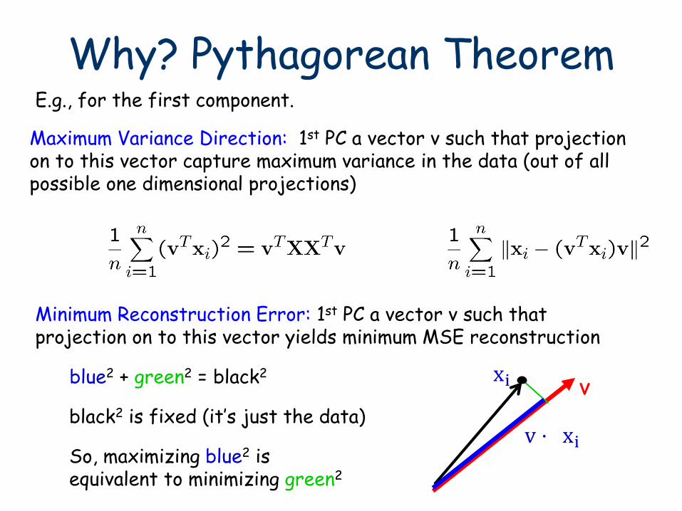
Why? Pythagorean Theorem

xi v

v ⋅ xi

blue2 + green2 = black2

black2 is fixed (it’s just the data)

So, maximizing blue2 is equivalent to minimizing green2

Maximum Variance Direction: 1st PC a vector v such that projection on to this vector capture maximum variance in the data (out of all possible one dimensional projections)

Minimum Reconstruction Error: 1st PC a vector v such that projection on to this vector yields minimum MSE reconstruction

E.g., for the first component.

Dimensionality Reduction using PCA

xi v

vTxi

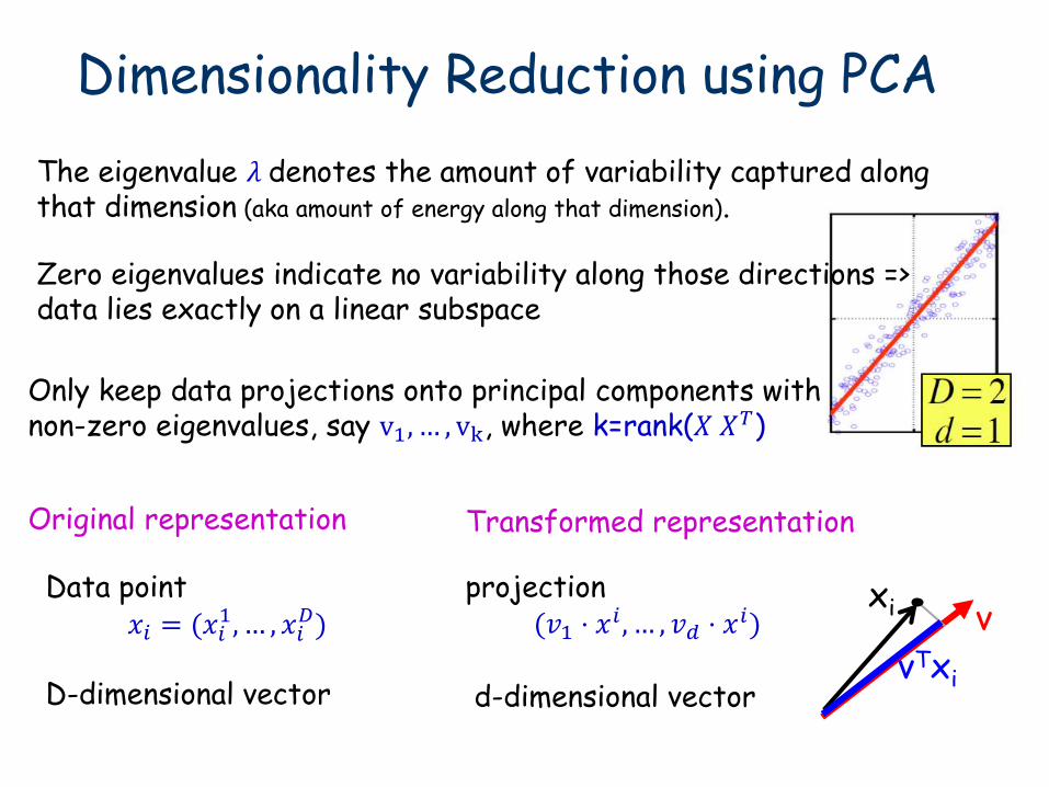
The eigenvalue 𝜆 denotes the amount of variability captured along that dimension (aka amount of energy along that dimension).

Zero eigenvalues indicate no variability along those directions => data lies exactly on a linear subspace

Only keep data projections onto principal components with non-zero eigenvalues, say v1, … , vk, where k=rank(𝑋 𝑋𝑇)

Original representation

Transformed representation

Data point

𝑥𝑖 = (𝑥𝑖1, … , 𝑥𝑖

𝐷)

projection

(𝑣1 ⋅ 𝑥𝑖 , … , 𝑣𝑑 ⋅ 𝑥𝑖)

D-dimensional vector

d-dimensional vector

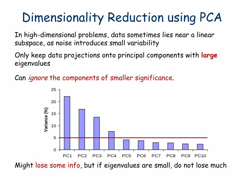
Dimensionality Reduction using PCA In high-dimensional problems, data sometimes lies near a linear subspace, as noise introduces small variability

Only keep data projections onto principal components with large eigenvalues

0

5

10

15

20

25

PC1 PC2 PC3 PC4 PC5 PC6 PC7 PC8 PC9 PC10

Var

ian

ce (

%)

Can ignore the components of smaller significance.

Might lose some info, but if eigenvalues are small, do not lose much

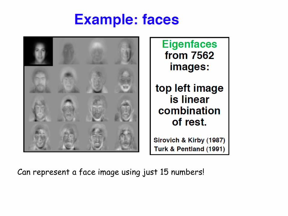
Can represent a face image using just 15 numbers!

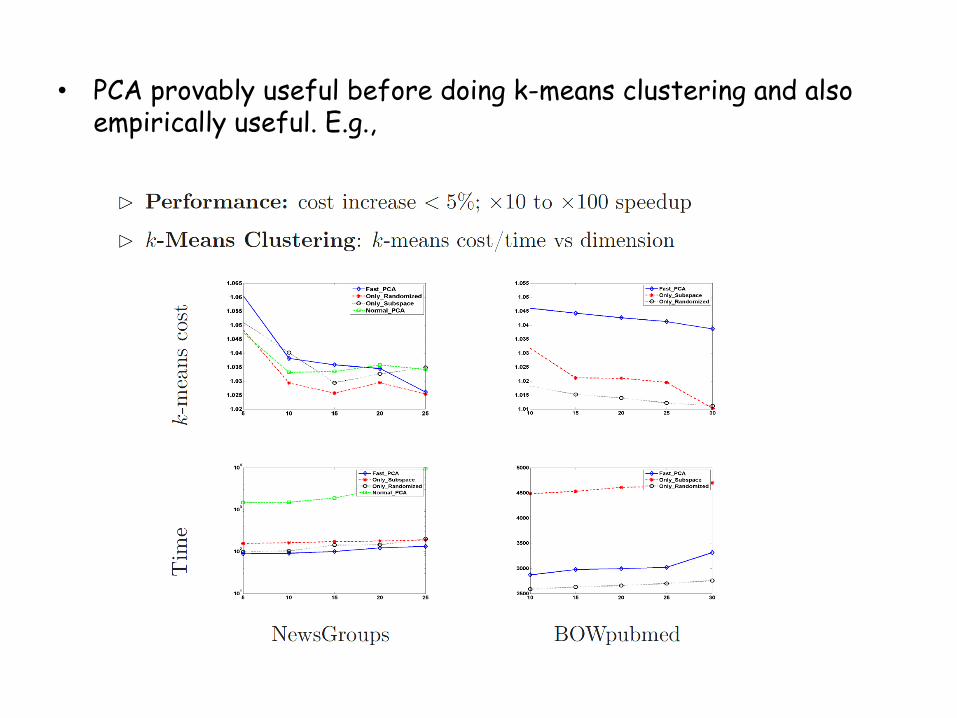
• PCA provably useful before doing k-means clustering and also empirically useful. E.g.,

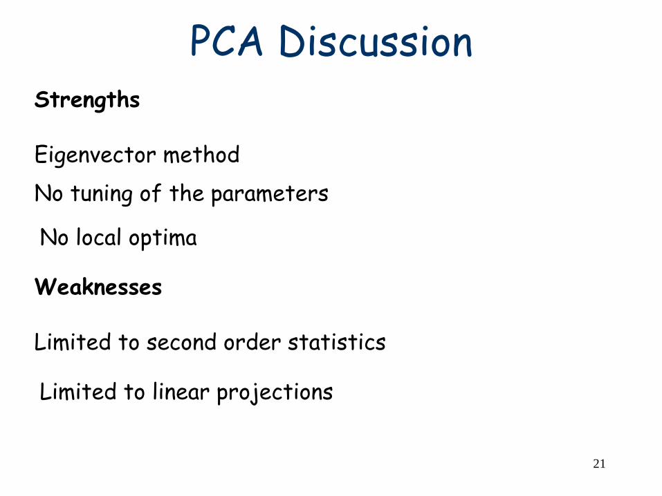
PCA Discussion Strengths

21

Eigenvector method

No tuning of the parameters

No local optima

Weaknesses

Limited to second order statistics

Limited to linear projections

Kernel PCA (Kernel Principal Component Analysis)

Useful when data lies on or near a low d-dimensional linear subspace of the 𝜙-space associated with a kernel

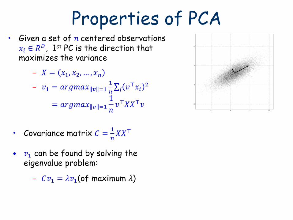
Properties of PCA • Given a set of 𝑛 centered observations

𝑥𝑖 ∈ 𝑅𝐷, 1st PC is the direction that maximizes the variance

– 𝐶𝑣1 = 𝜆𝑣1(of maximum 𝜆)

– 𝑋 = 𝑥1, 𝑥2, … , 𝑥𝑛

– 𝑣1 = 𝑎𝑟𝑔𝑚𝑎𝑥 𝑣 =11

𝑛 𝑣⊤𝑥𝑖

2𝑖

= 𝑎𝑟𝑔𝑚𝑎𝑥 𝑣 =1

1

𝑛𝑣⊤𝑋𝑋⊤𝑣

• Covariance matrix 𝐶 =1

𝑛𝑋𝑋⊤

• 𝑣1 can be found by solving the eigenvalue problem:

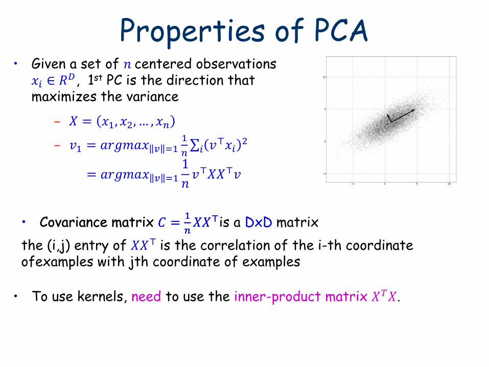
Properties of PCA

• Covariance matrix 𝐶 =1

𝑛𝑋𝑋⊤is a DxD matrix

the (i,j) entry of 𝑋𝑋⊤ is the correlation of the i-th coordinate ofexamples with jth coordinate of examples

• To use kernels, need to use the inner-product matrix 𝑋𝑇𝑋.

• Covariance matrix 𝐶 =1

𝑛𝑋𝑋⊤

• Given a set of 𝑛 centered observations 𝑥𝑖 ∈ 𝑅𝐷, 1st PC is the direction that maximizes the variance

– 𝑋 = 𝑥1, 𝑥2, … , 𝑥𝑛

– 𝑣1 = 𝑎𝑟𝑔𝑚𝑎𝑥 𝑣 =11

𝑛 𝑣⊤𝑥𝑖

2𝑖

= 𝑎𝑟𝑔𝑚𝑎𝑥 𝑣 =1

1

𝑛𝑣⊤𝑋𝑋⊤𝑣

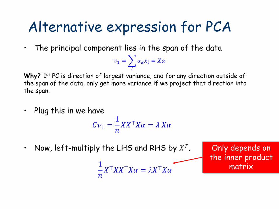
Alternative expression for PCA • The principal component lies in the span of the data

𝑣1 = 𝛼𝑘𝑥𝑖

𝑖

= 𝑋𝛼

Why? 1st PC is direction of largest variance, and for any direction outside of the span of the data, only get more variance if we project that direction into the span.

Only depends on the inner product

matrix

• Plug this in we have

𝐶𝑣1 =1

𝑛𝑋𝑋⊤𝑋𝛼 = 𝜆 𝑋𝛼

• Now, left-multiply the LHS and RHS by 𝑋𝑇.

1

𝑛𝑋⊤𝑋𝑋⊤𝑋𝛼 = 𝜆𝑋⊤𝑋𝛼

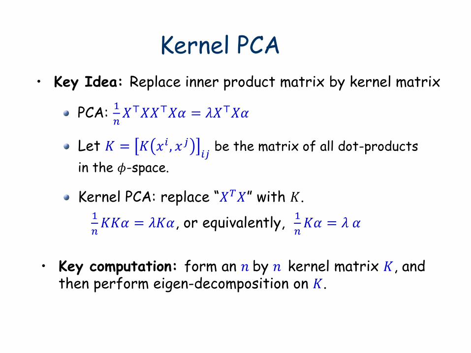
Kernel PCA

• Key Idea: Replace inner product matrix by kernel matrix

PCA: 1

𝑛𝑋⊤𝑋𝑋⊤𝑋𝛼 = 𝜆𝑋⊤𝑋𝛼

Let 𝐾 = 𝐾 𝑥𝑖 , 𝑥𝑗𝑖𝑗

be the matrix of all dot-products

in the 𝜙-space.

Kernel PCA: replace “𝑋𝑇𝑋” with 𝐾.

• Key computation: form an 𝑛 by 𝑛 kernel matrix 𝐾, and then perform eigen-decomposition on 𝐾.

1

𝑛𝐾𝐾𝛼 = 𝜆𝐾𝛼, or equivalently,

1

𝑛𝐾𝛼 = 𝜆 𝛼

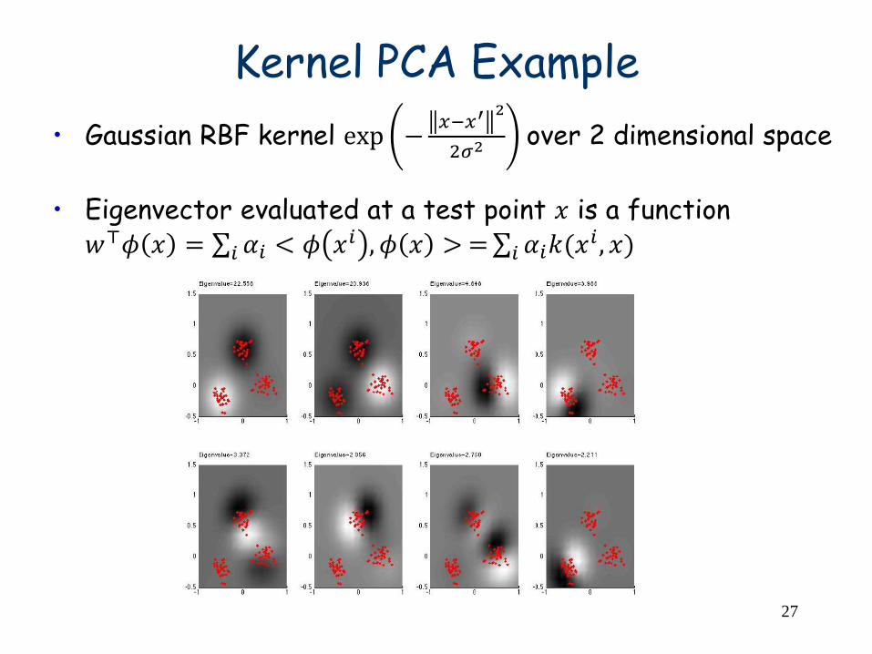
Kernel PCA Example

27

• Gaussian RBF kernel exp −𝑥−𝑥′ 2

2𝜎2 over 2 dimensional space

• Eigenvector evaluated at a test point 𝑥 is a function 𝑤⊤𝜙 𝑥 = 𝛼𝑖 < 𝜙 𝑥𝑖 , 𝜙 𝑥 > =𝑖 𝛼𝑖𝑘(𝑥

𝑖 , 𝑥)𝑖

What You Should Know

• Principal Component Analysis (PCA)

• Kernel PCA

• What PCA is, what is useful for.

• Both the maximum variance subspace and the

minimum reconstruction error viewpoint.

Additional material on computing the principal

components and ICA

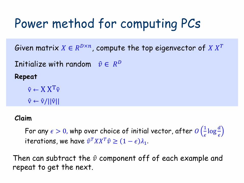
Power method for computing PCs

Given matrix 𝑋 ∈ 𝑅𝐷×𝑛, compute the top eigenvector of 𝑋 𝑋𝑇

Initialize with random 𝑣 ∈ 𝑅𝐷

Repeat

v ← X XTv

v ← v /||v ||

Claim

Then can subtract the 𝑣 component off of each example and repeat to get the next.

For any 𝜖 > 0, whp over choice of initial vector, after 𝑂1

𝜖log

𝑑

𝜖

iterations, we have 𝑣 𝑇𝑋𝑋𝑇𝑣 ≥ 1 − 𝜖 𝜆1.

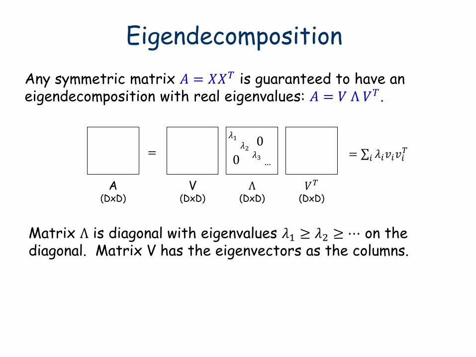
Eigendecomposition

Any symmetric matrix 𝐴 = 𝑋𝑋𝑇 is guaranteed to have an eigendecomposition with real eigenvalues: 𝐴 = 𝑉 Λ 𝑉𝑇 .

A (DxD)

=

V (DxD)

Λ (DxD)

𝜆1 𝜆2

𝜆3 …

0

0

𝑉𝑇 (DxD)

= 𝜆𝑖𝑣𝑖𝑣𝑖𝑇

𝑖

Matrix Λ is diagonal with eigenvalues 𝜆1 ≥ 𝜆2 ≥ ⋯ on the diagonal. Matrix V has the eigenvectors as the columns.

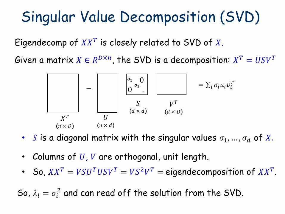
Singular Value Decomposition (SVD)

• 𝑆 is a diagonal matrix with the singular values 𝜎1, … , 𝜎𝑑 of 𝑋.

• Columns of 𝑈, 𝑉 are orthogonal, unit length.

So, 𝜆𝑖 = 𝜎𝑖2 and can read off the solution from the SVD.

Given a matrix 𝑋 ∈ 𝑅𝐷×𝑛, the SVD is a decomposition: 𝑋𝑇 = 𝑈𝑆𝑉𝑇

Eigendecomp of 𝑋𝑋𝑇 is closely related to SVD of 𝑋.

𝑋𝑇 (𝑛 × 𝐷)

=

𝑈 (𝑛 × 𝑑)

𝑆 (𝑑 × 𝑑)

𝜎1 𝜎2

…

0 0

𝑉𝑇 (𝑑 × 𝐷)

= 𝜎𝑖𝑢𝑖𝑣𝑖𝑇

𝑖

• So, 𝑋𝑋𝑇 = 𝑉𝑆𝑈𝑇𝑈𝑆𝑉𝑇 = 𝑉𝑆2𝑉𝑇 = eigendecomposition of 𝑋𝑋𝑇.

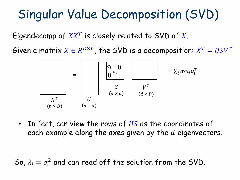
Singular Value Decomposition (SVD)

So, 𝜆𝑖 = 𝜎𝑖2 and can read off the solution from the SVD.

Given a matrix 𝑋 ∈ 𝑅𝐷×𝑛, the SVD is a decomposition: 𝑋𝑇 = 𝑈𝑆𝑉𝑇

Eigendecomp of 𝑋𝑋𝑇 is closely related to SVD of 𝑋.

𝑋𝑇 (𝑛 × 𝐷)

=

𝑈 (𝑛 × 𝑑)

𝑆 (𝑑 × 𝑑)

𝜎1 𝜎2

…

0 0

𝑉𝑇 (𝑑 × 𝐷)

= 𝜎𝑖𝑢𝑖𝑣𝑖𝑇

𝑖

• In fact, can view the rows of 𝑈𝑆 as the coordinates of each example along the axes given by the 𝑑 eigenvectors.

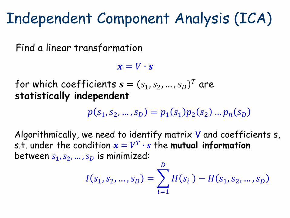
Independent Component Analysis (ICA)

𝑝 𝑠1, 𝑠2, … , 𝑠𝐷 = 𝑝1 𝑠1 𝑝2 𝑠2 …𝑝𝑛 𝑠𝐷

𝒙 = 𝑉 ∙ 𝒔

Find a linear transformation

for which coefficients 𝒔 = 𝑠1, 𝑠2, … , 𝑠𝐷𝑇 are

statistically independent

Algorithmically, we need to identify matrix V and coefficients s, s.t. under the condition 𝒙 = 𝑉𝑇 ∙ 𝒔 the mutual information between 𝑠1, 𝑠2, … , 𝑠𝐷 is minimized:

𝐼 𝑠1, 𝑠2, … , 𝑠𝐷 = 𝐻 𝑠𝑖 − 𝐻 𝑠1, 𝑠2, … , 𝑠𝐷

𝐷

𝑖=1

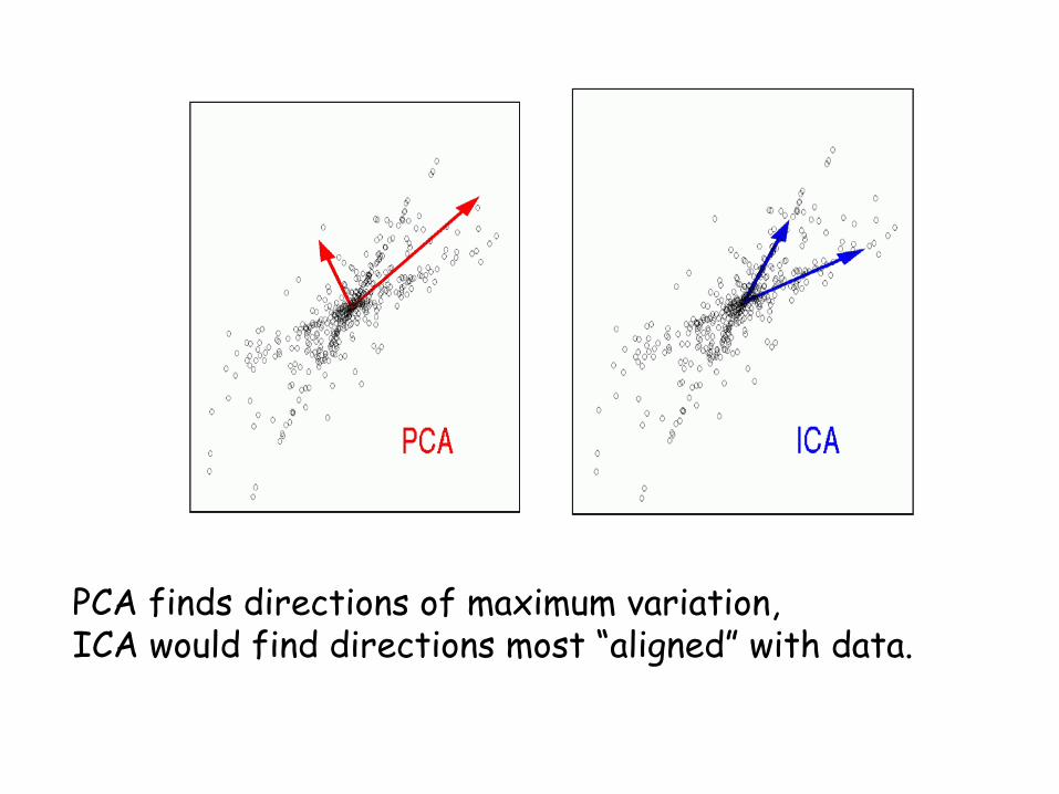
PCA finds directions of maximum variation, ICA would find directions most “aligned” with data.