Embed Size (px)
Citation preview
Copyright c© 2004 Tech Science Press CMES, vol.6, no.4, pp.373-395, 2004
PDE-Driven Level Sets, Shape Sensitivity and Curvature Flow for StructuralTopology Optimization
Michael Yu Wang1 and Xiaoming Wang2
Abstract: This paper addresses the problem of struc-tural shape and topology optimization. A level setmethod is adopted as an alternative approach to the pop-ular homogenization based methods. The paper focuseson four areas of discussion: (1) The level-set model ofthe structure’s shape is characterized as a region andglobal representation; the shape boundary is embedded ina higher-dimensional scalar function as its “iso-surface.”Changes of the shape and topology are governed by apartial differential equation (PDE). (2) The velocity vec-tor of the Hamilton-Jacobi PDE is shown to be naturallyrelated to the shape derivative from the classical shapevariational analysis. Thus, the level set method providesa natural setting to combine the rigorous shape variationsinto the optimization process. (3) Perimeter regulariza-tion is incorporated in the method to make the optimiza-tion problem well-posed. It also produces an effect ofthe geometric heat equation, regularizing and smoothingthe geometric boundaries as an anisotropic filter. (4)Wefurther describe numerical techniques for efficient androbust implementation of the method, by embedding arectilinear grid in a fixed finite element mesh defined ona reference design domain. This would separate the is-sues of accuracy in numerical calculations of the physicalequation and in the level-set model propagation. Finally,the benefit and the advantages of the developed methodare illustrated with several 2D examples that have beenextensively used in the recent literature of topology opti-mization, especially in the homogenization based meth-ods.
keyword: Topology optimization, level set method,shape sensitivity, curvature flow
1 Department of Automation and Computer-Aided Engineering,The Chinese University of Hong Kong, Shatin, NT, HongKong. Tel.: +852-2609-8487; Fax: +852-2603-6002. E-mail:[email protected] (M. Y. Wang).
2 School of Mechanical Engineering Dalian University of Technol-ogy Dalian 116024, China
1 Introduction
Structural optimization, in particular the shape and topol-ogy optimization, has been identified as one of the mostchallenging tasks in structural design. Various tech-niques have been developed in the past decades. Typi-cal procedures are based on an explicit boundary repre-sentation with a fixed topology of the structure (Bendsoe(1997); Rozvany (1998); Sokolowski et al. (1992)). Inthe direct approach, the problem of structural optimiza-tion is a well-posed mathematical problem, and numeri-cal algorithms can be developed based on rigorous analy-ses for shape sensitivity and necessary optimality condi-tions (Haug et al. (1986); Sokolowski et al. (1992)). As aresult, these optimization procedures are widely availablein commercial finite element software systems. However,these procedures do not admit changes in the connectiv-ity of the geometry of the structure, imposing a signif-icant constraint on the design and thus limiting the po-tential of the structural performance. Perhaps as a ma-jor motivation to overcome the fixed-topology limitation,the concept of topology optimization has been introducedin recent years (Bendsoe (1989, 1997); Bendsoe et al.(1988, 1993)), often with a “raster” geometric model of arefined finite element grid covering the candidate designdomain. Over the past decade, there have been some ex-tensive developments of various approaches to this prob-lem.
Unfortunately, the problem of topology optimization of astructure is an ill-posed problem in its mathematical the-ory and numerical methods (Haber et al. (1996)). Asfirst observed numerically in (Cheng et al. (1981)) fora variable-thickness plate design problem, the optimiza-tion problem may not admit a solution. Particularly forthe problem of minimizing the structural compliance ofan elastic body for a specified set of loads and supports,it has been illustrated that a non-convergent design se-quence can be constructed such that the compliance re-duces monotonically (Bendsoe (1997)). The resulting
374 Copyright c© 2004 Tech Science Press CMES, vol.6, no.4, pp.373-395, 2004
design has a configuration with an unbounded number ofmicroscopic holes, rather than a finite number of macro-scopic holes.
For the reason to generate a well-posed topology opti-mization problem, the so-called homogenization methodhas been extensively developed in recent years andevolved into the state-of-the-art (Bendsoe (1989, 1997);Bendsoe et al. (1988, 1993)). In this approach, the de-sign space is first extended to explicitly include mate-rials with periodic, perforated microstructures and thenhomogenization theory is utilized to compute effectivematerial properties. This procedure is known as relax-ation and, as a result, solutions to the relaxed problemare guaranteed to exist. A “side-effect” of the relaxationis that the optimal solutions generated by homogeniza-tion methods commonly have perforated microstructuresin the resulting design, as expected in consistence withthe relaxation. Unfortunately, perforated microstructuresare difficult to manufacture. Thus, the “relaxed” optimalsolutions may not lead directly to useful designs.
Therefore, it becomes necessary to be able to suppressperforated microstructures in the optimal design by mod-ifying the relaxed formulation. Several suppression tech-niques have been developed. Introducing a priori re-strictions on the configuration of the microstructure isan approach presented in (Bendsoe (1997); Bendsoe etal. (1988)), while the suppression may also be achievedby explicitly penalizing intermediate values of the bulkdensity. The later technique becomes quite popular, es-pecially with the “solid isotropic material with penaliza-tion” (SIMP) approach for its conceptual and practicalsimplicity (Bendsoe (1997); Mlejnek (1992); Rozvany(2001)). It has been pointed out that certain configurationrestrictions are equivalent to explicit penalties on inter-mediate densities (Bendsoe et al. (1999)), thus yieldingsimilar designs. Various “engineering approaches” havealso been suggested, including adding more constraintsinto the problem such as perimeter controls (Petersson(1999)) and slope constraints (Petersson et al. (1998)),and employing filters for chattering solutions (Bourdin(2001); Sigmund (2000, 2001); Sigmund et al. (1998);Wang and Zhou (2004); Tapp et al. (2004)). Althoughthese suppression techniques have been widely appliedto problems with multiple physics and multiple materials(Bendsoe (1997); Bourdin (2001); Bulman et al. (2001);Rozvany (2001); Suzuki et. al. (1991)), the solutions areoften mesh dependent. Further, numerical instabilities
are inherent and may introduce “non-physical” artifactsin the results to make the designs sensitive to variations inthe physical and numerical parameters of the system suchas loading (Bourdin (2001); Bulman et al. (2001); Roz-vany (2001); Sigmund et al. (1998)). The suppressionsdo not directly address the chattering problem underlyingthe relaxation concept.
An alternative approach for generating a well-posedtopology optimization problem is to define the designspace to exclude chattering designs (Ambrosio et al.(1993); Larsen et al. (2001)). A common approach isto introduce an upper bound constraint on the perimeterof the design (Haber et al. (1995)). A numerical investi-gation of the “perimeter constraint method” was givenin (Haber et al. (1995)), which shows that a perime-ter constraint can effectively exclude perforated materialand result in a well-posed macroscopic design. A morefundamental approach is to use the perimeter as a pe-nalization for regularizing the ill-posedness of the topol-ogy optimization problem. A mathematical analysis ofthe perimeter regularization method was first presentedin (Ambrosio et al. (1993)). Other studies also providemore mathematical support for the approach (Larsen etal. (2001)), which in fact has been extensively utilizedin the field of digital image processing over the years(Sapiro (2001)).
Another essential feature of most of the existing topol-ogy optimization approaches is the “raster” geometricmodel. A finite element grid is used both for represent-ing the structure and for physical analysis of the struc-tural mechanics. In the final optimal design, an effectiveindicator value of either 0 or 1 (or in between) is obtainedfor each element to define the design geometry implicitly.In the end, the designer must interpret the resulting dis-tribution and extract the boundaries of the solid region(Lin et al. (2000)). This is in contrast to the boundarymodels that are commonly used in finite element proce-dures for shape optimization. Boundary representationsare always essential for design description and for designautomation with CAD and CAE systems. These funda-mental issues are still argued in the literature (Rozvany(2001)).
Adopting the same spirit of using boundary-representation geometric models, a new approachwas recently proposed using the versatile level-setmodels (Osher et al. (2001); Sethian et al. (2000);Wang et al. (2003); Sheen et al. (2003)). The level
Structural Topology Optimization 375
set method was developed in (Osher et al. (2003)) toprovide an efficient way of describing time evolvingcurves and surfaces which may undergo topologicalchanges. It has been recognized that the level-set modelsare well suited to the structural topology optimization,as they can form holes, split into multiple pieces, ormerge with others to form a single one (Osher et al.(2001); Wang et al. (2003); Wang et al. (2004)). Theyare used in (Sethian et al. (2000)) to accommodate anevolutionary procedure of removing (or adding) materialin regions according to the stress levels computed withan explicit jump immersed interface method withoutusing meshes. The general topology optimizationproblem can be formulated as a problem of tracking thegeometric boundaries as motion of level sets driven bythe optimization conditions (Allaire et al. (2002); Wanget al. (2003); Wang et al. (2004)).
In this paper we address the topology optimization prob-lem of a linearly elastic structure with the level-set for-mulation. For a given design objective and a set of con-straints, a global minimization criterion is introduced,consisting of the design objective and a perimeter penaltyproportional to the Hausdorff measure of the designboundary. In using the level-set model, the boundary ofthe structure is embedded in a scalar function of a higherdimensionality. Based on the level set theory, the dy-namic change of the structural boundary is governed bya partial differential equation (PDE) of Hamilton-Jacobitype. Thus, the topology optimization is described as asolution of the Hamilton-Jacobi equation. More specif-ically, the paper focuses on the following three areas ofdiscussions:
1. Evolution of geometric boundary embedded in ahigher-dimensional space. The level set model is de-fined as a region representation of the structure’s shape.A comprehensive understanding of the structural shapeinvolves both the notions of its boundary and its in-terior. While the classical shape optimization has fo-cused mainly on the process of changing the boundariesof the shape, the modern notion of topology optimiza-tion captures the regions bounded by the boundaries.The level set model provides this extra “dimension” ofinformation by allowing for an evolution of the three-dimensional boundaries in a higher four-dimensionalspace constrained to embed the original problem. Thepermissible changes of the boundaries are further con-strained by the dynamic motions of the level sets defined
by their partial differential equations. Within this globaland region-based framework, the topology optimizationof the structure is transformed into a process of motionof the PDE-driven level-set.
2. The velocity field in level-set evolution and theclassical shape derivative. We will further examine therole of the velocity field in the Hamilton-Jacobi equationand its relationship to the shape derivative of the classicalshape optimization. We will show that the shape deriva-tive defined in the framework of shape diffeomorphismis naturally associated with the flow of the velocity fieldof the evolution of the level set model. Thus, the levelset representation can be naturally combined with an ap-plication of the classical shape analysis. Such a combi-nation provides a proper and determinant choice of thevelocity field to lead a convergent process of minimizingthe objective functional.
3. Perimeter regularization and curvature-based diffu-sion. We will study the regularizing effect of the perime-ter penalty for the topology optimization problem. Theprimary effect of a perimeter penalization is that it en-sures the existence of smooth solutions. For the levelset representation, this effect is shown to be equivalentto curvature diffusion. In other words, the regulariza-tion effect can be viewed as running the geometric shapethrough a nonlinear heat equation. Since the geometricheat equation may be regarded as a nonlinear Guassiansmoothing process, the perimeter regularization can alsobe related to an anisotropic filtering which gives a num-ber of advantages as widely used in imaging processing.
4. Numerical computations for approximated solu-tions. We shall describe numerical techniques for effi-cient and robust implementation of the proposed method.Since it is convenient to numerically solve the level setPDE with a fixed rectilinear spatial grid, we suggest thatsuch a grid is embedded as nodes in a finite element meshwhich is defined in a fixed reference domain for numeri-cal calculations of the linear elastic system. This schemewould allow for a complete separation in the accuracyof the geometric model and the accuracy of numericalcalculations of the physical system. A local computa-tion scheme can be used to keep the computational com-plexity linear to the complexity of the physical boundaryof the structure, while either first order or higher orderapproximation methods are available for the space-timediscretization.
We have developed a numerical implementation of the
376 Copyright c© 2004 Tech Science Press CMES, vol.6, no.4, pp.373-395, 2004
level set method for the structural optimization problem.The benefit and the advantages of the proposed methodare illustrated with several 2D examples that have beenextensively used in the recent literature of topology opti-mization, especially in the homogenization based meth-ods.
2 The Optimization Problem
In this paper we use a linear elastic structure to describethe problem of structural optimization. Conceptually,the approach presented here would apply to a generalstructure model. Let Ω ⊆ Rd (d = 2 or 3) be an openand bounded set occupied by a linear isotropic elasticstructure. The boundary of Ω consists of three parts:Γ = ∂Ω = Γ0 ∪Γ1 ∪Γ2, with Dirichlet boundary condi-tions on Γ1 and Neumann boundary conditions on Γ2. Itis assumed that the boundary segment Γ0 is traction free.The displacement field u in Ω is the unique solution ofthe linear elastic system
−div σ(u) = f in Ωu = u0 on Γ1
σ(u) ·n = h on Γ2 (1)
where the strain tensor ε and the stress tensor σ at anypoint x ∈ Ω are given in the usual form as
ε(u) =12
(∇u+∇uT )
σ(u) = Eε(u) (2)
with E as the elasticity tensor, u0 the prescribed displace-ment on Γ1, f the applied body force, h the boundarytraction force applied on Γ2 such as an external pressureload exerted by a fluid, and n the outward normal to theboundary.
The general problem of structure optimization is speci-fied as
MinimizeΩ
Q(u,Ω) =∫
ΩF (u)dΩ+µ |∂Ω|
sub ject to :∫
ΩdΩ ≤ M (3)
where |∂Ω| is the Hausdorff measure of the boundary, orperimeter of ∂Ω and µ is a positive parameter. The in-equality describes the limit on the amount of material interms of the maximum admissible volume M of the de-
sign. The variational equation of the linear elastic equi-librium is written as∫
ΩEε(u) : ε(v)dΩ
=∫
Ωf · vdΩ+
∫Γ2
h · vdΓ, for all v ∈U
U =
u : u ∈ H1 (Ω) ; u = u0 on Γ1
(4)
with U denoting the space of kinematically admissibledisplacement fields and ‘:’ representing the second or-der tensor operator. The goal of optimization is to finda minimizer Ω for the global criterion Q(u,Ω) whichyields an optimized structure with respect to a specificfunction described by F (u). This is a standard notionof structural optimization (Bendsoe (1997); Sethian etal. (2000)) augmented with the perimeter regularization(Ambrosio et al. (1993)).
The design function F (u) may involve any physical orgeometric quantity of the design. While the most com-mon choice for F (u) might be the mean compliance ofthe structure, i.e.,
J(u,Ω)≡∫
ΩF (u)dΩ =
∫Ω
Eε(u) : ε(u)dΩ (5)
it may deal with a stress consideration F (σ(u)) or a dis-placement function F (u,x0) = u(x)δ(x−x0) for x, x0 ∈Ω and δ(·) being the Dirac delta function.
A fundamental question regarding this class of struc-tural optimization problems (3) is about the existence andsmoothness of the solutions. The issue and its signifi-cance has been a subject of extensive studies in a classof more general problems of domain identification withregularization (Bourdin et al. (2000); Chenais (1975)).For the structural problems of displacement fields satis-fying the linear elasticity system, the issue has been in-vestigated in (Ambrosio et al. (1993); Bourdin (2000);Larsen (2001)) with some substantial analysis resultssuggesting that this class of perimeter-regularized prob-lems are well-posed with the existence of smooth solu-tions. While the mathematical analyses are yet com-plete, various numerical experiences seem to confirm thatthe problem formulation provides a well-behaved frame-work for seeking meaningful optimal solutions, particu-larly when the models of the structure have finite perime-ter. The level set model is indeed such a model as to bepresented next.
Structural Topology Optimization 377
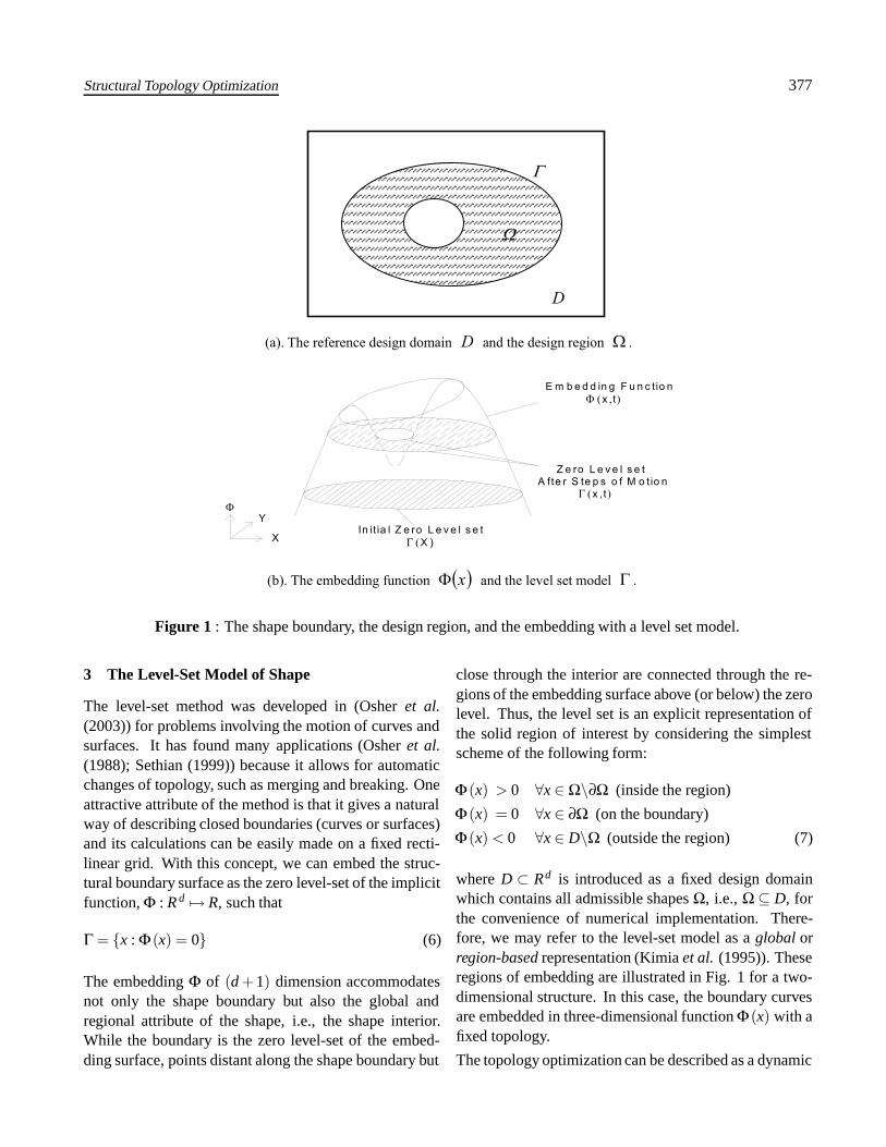
(a). The reference design domain D and the design region .
D
In it ia l Z e ro L e v e l s e t
X )
E m b e d d in g F u n c tio n
x t
Z e ro L e v e l s e t A fte r S te p s o f M o tio n x , t
X
Y
(b). The embedding function x and the level set model .
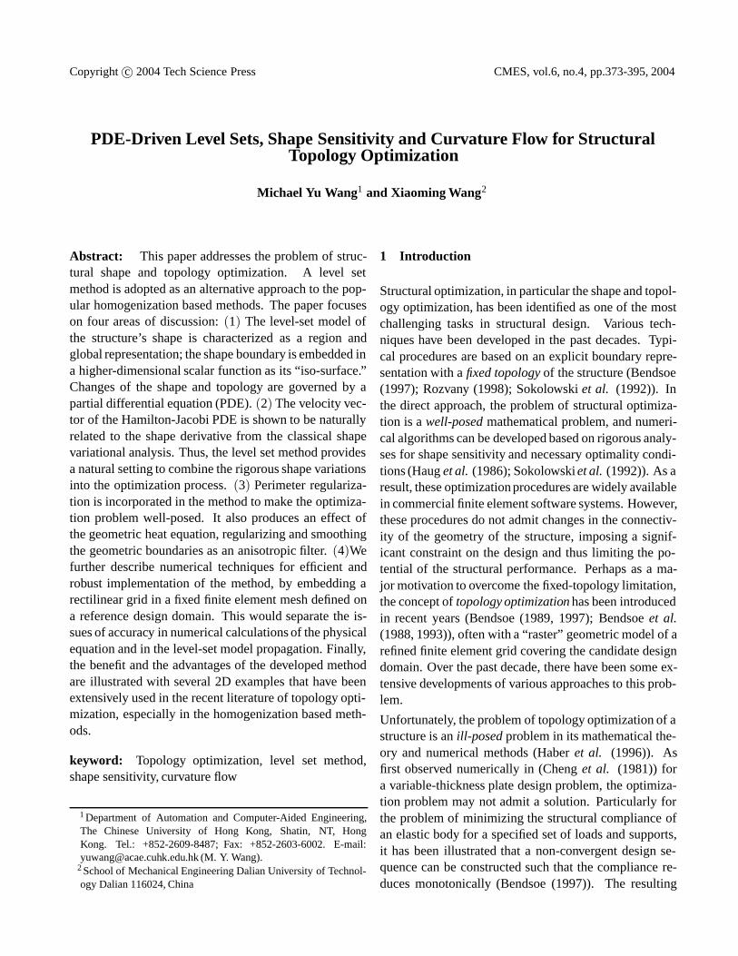
Figure 1 : The shape boundary, the design region, and the embedding with a level set model.
3 The Level-Set Model of Shape
The level-set method was developed in (Osher et al.(2003)) for problems involving the motion of curves andsurfaces. It has found many applications (Osher et al.(1988); Sethian (1999)) because it allows for automaticchanges of topology, such as merging and breaking. Oneattractive attribute of the method is that it gives a naturalway of describing closed boundaries (curves or surfaces)and its calculations can be easily made on a fixed recti-linear grid. With this concept, we can embed the struc-tural boundary surface as the zero level-set of the implicitfunction, Φ : R d → R, such that
Γ = x : Φ (x) = 0 (6)
The embedding Φ of (d +1) dimension accommodatesnot only the shape boundary but also the global andregional attribute of the shape, i.e., the shape interior.While the boundary is the zero level-set of the embed-ding surface, points distant along the shape boundary but
close through the interior are connected through the re-gions of the embedding surface above (or below) the zerolevel. Thus, the level set is an explicit representation ofthe solid region of interest by considering the simplestscheme of the following form:
Φ (x) > 0 ∀x ∈ Ω\∂Ω (inside the region)
Φ (x) = 0 ∀x ∈ ∂Ω (on the boundary)
Φ (x) < 0 ∀x ∈ D\Ω (outside the region) (7)
where D ⊂ Rd is introduced as a fixed design domainwhich contains all admissible shapes Ω, i.e., Ω ⊆ D, forthe convenience of numerical implementation. There-fore, we may refer to the level-set model as a global orregion-based representation (Kimia et al. (1995)). Theseregions of embedding are illustrated in Fig. 1 for a two-dimensional structure. In this case, the boundary curvesare embedded in three-dimensional function Φ (x) with afixed topology.
The topology optimization can be described as a dynamic
378 Copyright c© 2004 Tech Science Press CMES, vol.6, no.4, pp.373-395, 2004
process of level set changing in pseudo-time t. The sur-face of the embedding function may move up and downon a fixed coordinate system without ever altering itstopology. The structural boundary embedded on Φ (x)can undergo drastic topological changes. However, thereis no need to directly track these structural topologicalchanges. The evolution of the implicit function Φ (x) isobtained by differentiating both sides of (6) with respectto time and by applying the chain rule, yielding the sim-ple Hamilton-Jacobi convection equation
∂Φ (x)∂t
+∇Φ (x) ·V (x) = 0 (8)
where V (x) is the velocity vector of x and it is often re-ferred to as the velocity function of the level-set evolu-tion, i.e.,
V (x) =dxdt
(9)
Furthermore, by definition of (7), we have n =−∇Φ
/|∇Φ| with |∇Φ| = (∇Φ ·∇Φ)1/2, and ∇Φ ·V =−(V ·n) |∇Φ|. Then, equation (8) can be written as
∂Φ (x)∂t
= Vn |∇Φ (x)| Vn = V ·n (10)
This is known as the level set equation (Osher et al.(1998, 2003); Sethian (1999)).
Several features and advantages of this method represent-ing the unknown solid shape through the level-set func-tion Φ (x) become apparent:
1. First, level set models are topologically flexible.The scalar function Φ is defined to always have a simpletopology; the representation does not rely on any kind ofexplicit parameterization. The shape representation is asgeneral as the underlying physical theory. These capabil-ities would allow the boundary models to easily changethe structural topology while undergoing optimization inthat they can form holes, split to form multiple bound-aries, or merge with other boundaries to form a singlesurface, in contrast to any conventional boundary shapedesign (Sethian (1999)).
2. Since the geometric shape is constrained to be thezero level-set of the embedding function Φ (x), motion ofthe level set in (10) is permitted only along the normal di-rection of Φ (x), driven by the normal velocity Vn =V ·n.Therefore, the change in the embedded geometric shape
is also only in its normal direction. It is well knownin differential geometry (Kimia et al. (1995); Sapiro(2001)) that for a general velocity vector V = dx
/dt its
tangential component does not influence the geometry ofthe shape deformation; it changes only its parameteriza-tion. Therefore, the level set equation will not change theparameterization of the solid shape; the level set formu-lation is a parameterization free formulation.
3. In the classical shape optimization theory, thereexists an important concept of velocity field of shape de-formation (Haug et al. (1986); Sokolowski et al. (1992)).Based on ideas of continuum mechanics, it has beenfound that shape derivatives for a diffeomorphism per-turbation of a solid exist only in the normal direction ofthe geometric boundary. The underlying principle of theclassical shape optimization is to find a suitable choiceof the normal velocity field Vn = V · n to ensure a con-vergent sequence for the optimal solution. Clearly, thelevel set model provides a natural way to accommodatethis requirement. We need to enforce the velocity func-tion Vn in the level set equation to ensure a decrease ofthe objective functional Q(u,Ω) such that it is necessarythat Vn (x) = 0 everywhere on the design boundary Γ atan optimal solution. This will be discussed in detail innext section.
4. Further, a number of numerical techniques havebeen developed (Osher et al. (1998, 2003); Sethian(1999)) to make the initial value problem of (10) com-putationally robust and efficient. In fact, in the generalcase of a three dimensional solid structure, the compu-tational complexity can be made proportional to the sur-face area of the structure rather than the size of its vol-ume. The solutions to the level-set PDE can be accuratelycomputed even when the boundary is not smooth and sin-gularities develop in classical derivatives (Sapiro (2001);Sethian (1999)). This robust property is determined bythe unique entropy condition of the Hamilton-Jacobi con-vection equation (Osher et al. (2003)).
With the level set model we can describe the topologyoptimal problem in terms of the scalar function Φ. It ismost convenient to use the Heaviside function H and theDirac delta function δ defined as
H (Φ) =
1 if Φ ≥ 00 if Φ < 0
and δ(Φ) =dHdΦ
(11)
Therefore, the optimization problem is now written as
Structural Topology Optimization 379
follows:
MinimizeΦ
Q(u,Φ)
=∫
DF (u)H (Φ)dΩ+µ
∫D
δ(Φ) |∇Φ|dΩ
sub ject to : g(Φ) =∫
DH (Φ) dΩ − M ≤ 0 (12)
while the variational equation is written in the energy bi-linear and the load linear form as
a(u,v,Φ) = L(ν,Φ) (13)
where
a(u,v,Φ) =∫
DEε(u) : ε(v)H(Φ)dΩ
L(v,Φ) =∫
D( f · v)H(Φ)dΩ +
∫D
(h · v)δ(Φ) |∇Φ|dΩ
(14)
It is useful to note that
|∂Ω| =∫
ΓdΓ =
∫D
δ(Φ) |∇Φ|dΩ
4 Shape Derivative and Velocity Field
4.1 Material Derivatives
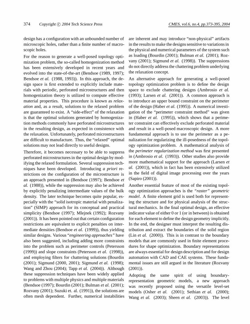
In the classical shape optimization theory, shape deriva-tive is an important concept as it relates a variation in theshape with the resulting variation in the objective func-tional. In this case, the design variable is not a functionbut the direct shape of a geometric domain Ω. (Haug etal. (1986); Sokolowski et al. (1992)). In order to definethe shape derivative, it is convenient to treat Ω. as a con-tinuous medium and to use the material derivative idea ofcontinuum mechanics (Haug et al. (1986)). Shape defor-mation can be viewed as a transformation defined by themapping T : x → xt (x) , x ∈ Ω, such that
xt = T (x, t) Ωt = T (Ω, t) (15)
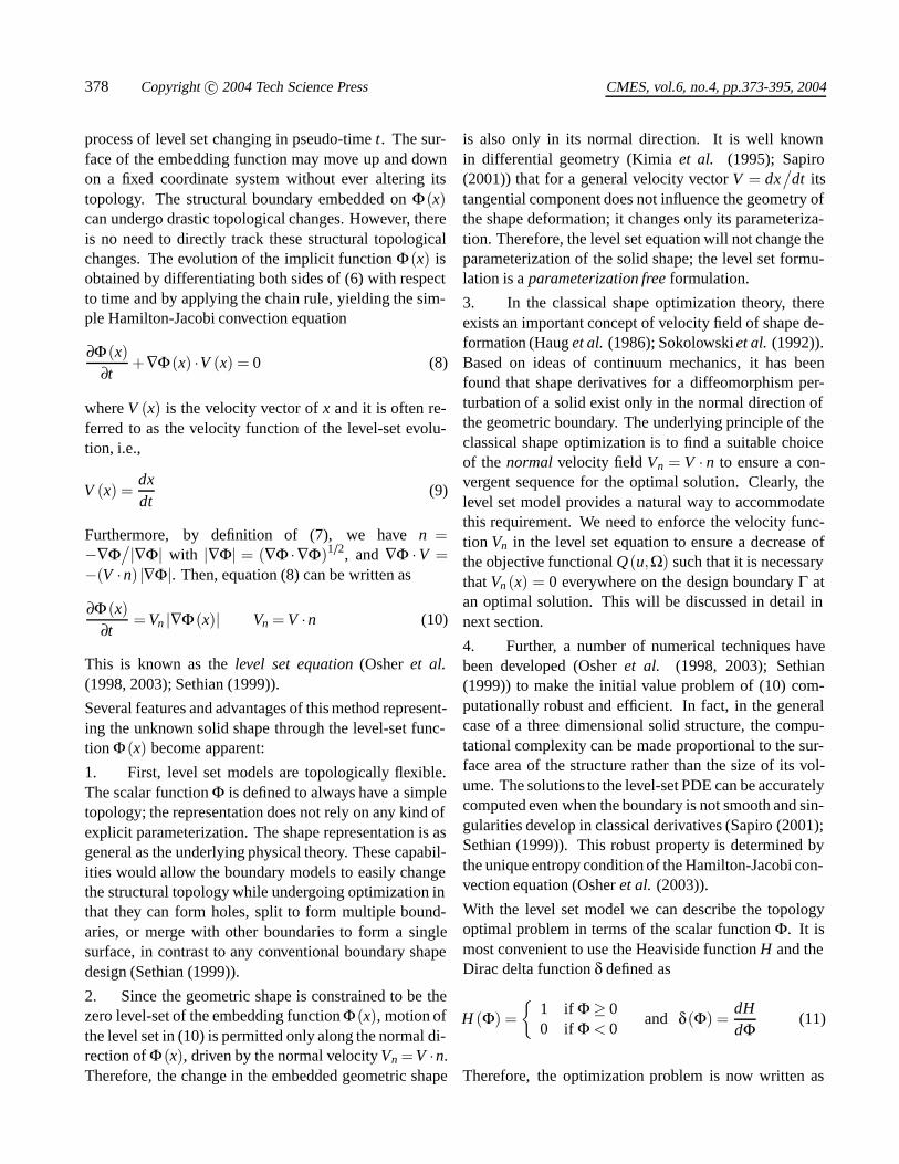
This mapping may be regarded as a dynamic process ofdeforming the shape with pseudo-time t as illustrated inFig. 2. In a more general method, this transformation canbe represented by its velocity
V (xt , t) =dxt
dt
xt
x
n
tV
tVn
t
Figure 2 : Shape mapping and variation of shape.
Under sufficient regularity conditions, such as that T −1
exists, then the velocity field is given by
V (xt , t) =∂T∂t
T−1 (xt , t)
Therefore, the shape deformation can be described by theinitial-value problem
dxt
dt= V (xt , t) x0 = x (16)
This shape deformation analysis leads to the so-called Lagrangian formulation of boundary propagation(Sokolowski et al. (1992)). When the steady state ofthis equation is achieved (i.e.,dxt
/dt = 0), an optimal
shape of the structure is obtained (Haug et al. (1986));Sokolowski et al. (1992)). The method has been ex-tensively studied and there are well-established numeri-cal implementations and software systems for boundaryshape design (Haug et al. (1986)). Unfortunately, thisformulation has a sever limitation that only geometry ofa fixed topology can be handled. In contrast, our level setequation (10) is known as the Eulerian formulation of theboundary propagation since the boundary is captured bythe implicit function Φ (x).
Within this context, the shape transformation is definedby the identity
xt = T (x, t) = x+ tV (x) V (x) = V (x,0) (17)
380 Copyright c© 2004 Tech Science Press CMES, vol.6, no.4, pp.373-395, 2004
This diffeomorphism was introduced by Murat and Si-mon (see, e.g., (Sokolowski et al. (1992)). Thus, aunique velocity field is given as similar to what is de-fined in the level-set equation (10). Since our global costQ(u,Φ) is a functional that depends on the displacementfield u and on the shape domain Ω rather than a directfunction, we need to use the concept of material deriva-tives in order to derive the shape derivative of the objec-tive functional (Haug et al. (1986)). A comprehensiveanalysis of the concept has been extensively describedin the literature (Haug et al. (1986); Sokolowski et al.(1992)). We shall utilize three most relevant lemmasthat are presented in Appendix. The reader is referredto (Haug et al. (1986)) for their proofs.
4.2 Shape Derivative of the Objective Functional
For a given velocity vector V , we now can find the shapederivative of an objective functional. First, we take thematerial derivative of both sides of the variational equa-tion (14). For the self-adjoint energy bilinear form
a(u,v,Ω) =∫
ΩEε(u) : ε(v)dΩ
we obtain the following form, by applying Lemma 1,
a ′ (u,v,Ω)
=∫
ΩEε(u) : ε(v)dΩ +
∫Γ
Eε(u) : ε(v) (V ·n)dΓ (18)
For the load linear form,
l (v,Ω) =∫
Ωf · vdΩ +
∫Γ2
h · vdΓ
we consider first the conservative loading in which thetraction h in (4) depends on position only. ApplyingLemma 1 and Lemma 2, it yields the following materialderivative
l′ (v,Ω)
=∫
Γ( f · v) (V ·n)dΓ
+∫
Γ2
(∇(h · v) ·n+κh · v) (V ·n)dΓ (19)
We can also consider the more general non-conservativeloading case. For example, the traction force of pressureloading in (4) is given as
h(x) = −p(x)n(x) , x ∈ Γ2 (20)
Then the material derivative becomes the following, us-ing Lemma 3,
l′ (v,Ω)
=∫
Γ( f · v)(V ·n)dΓ −
∫Γ2
(div(pv)) (V ·n)dΓ (21)
Further, consider our optimization objective functional inthe general form
J(u,Ω)≡∫
ΩF (u)dΩ
Its Eulerian derivative in the direction of the velocity vec-tor V is obtained by applying Lemma 1, such that,
J′(u,Ω)≡ dJ (Ω,V)/
dt
=∫
ΩF ′ (u) udΩ+
∫Γ
F (u) (V ·n)dΓ (22)
Finally, the general variable formulation gives rise to thefollowing adjoint equation
a(u,v) =∫
ΩF ′ (u) udΩ (23)
Thus, equating (18) with (19) and (21) respectively andthen using (22) and (23), we obtain the Eulerian deriva-tive of the objective functional, respectively for the con-servative traction loading as,
J ′(u,Ω)
=∫
Γ[F (u)+ f · v+κh · v+∇(h · v) ·n−Eε(u) : ε(v)]
(V ·n)dΓ (24)
and for the non-conservative loading of pressure tractionas,
J ′(u,Ω)
=∫
Γ[F (u)+ f · v−div(pv)−Eε(u) : ε(v)] (V ·n)dΓ
(25)
Therefore, this derivative can then be expressed in termsof the level set model Φ as
J ′(u,Φ) =∫
Ωδ(Φ)G(Φ)Vn |∇Φ|dΩ (26)
Structural Topology Optimization 381
where, respectively
G(u,v,Φ)= −(F (u)+( f +κh) · v+∇(h · v) ·n−Eε(u) : ε(v))
and
G(u,v,Φ)= −(F (u)+ f · v−div(pv)−Eε(u) : ε(v))
In the gradient of the objective functional (26) G(u,Ω) isknown as the shape gradient density (Haug et al. (1986)).Here, we use the identity that dΓ = δ(φ) |∇φ|dΩ andthe fact that Γ = x : Φ (x) = 0 in changing the bound-ary integral into the use of the level set geometric rep-resentation. Also, n(Φ) = −∇Φ
/|∇Φ| and κ(Φ) =−∇ · (∇Φ
/|∇Φ|).
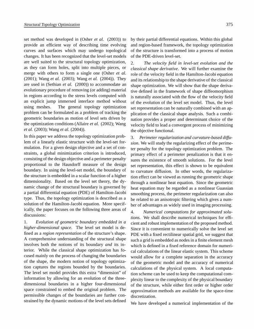
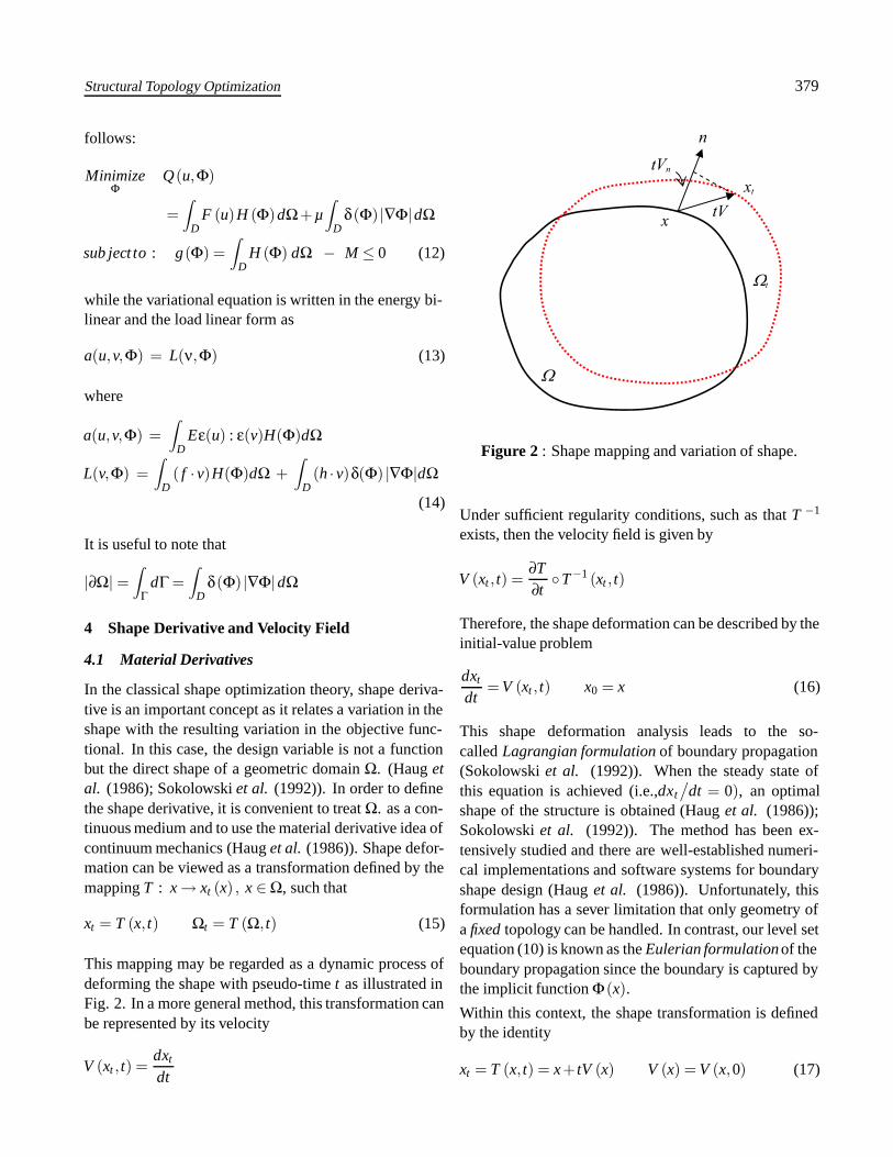
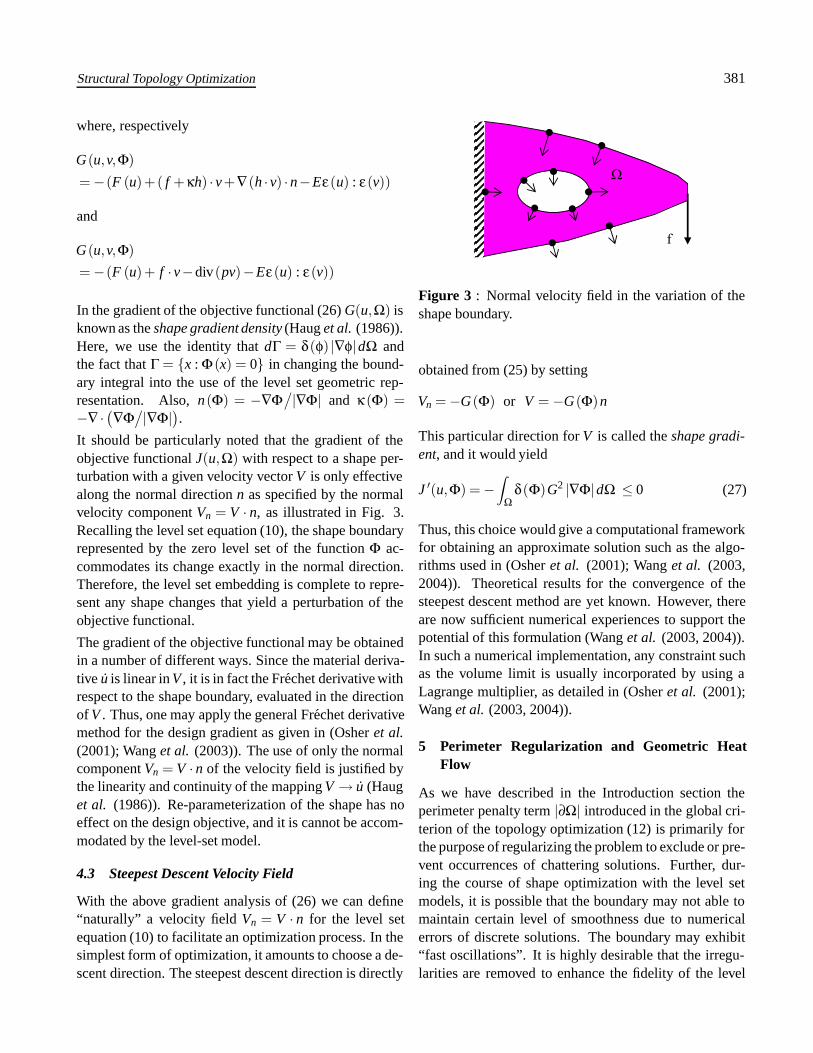
It should be particularly noted that the gradient of theobjective functional J(u,Ω) with respect to a shape per-turbation with a given velocity vector V is only effectivealong the normal direction n as specified by the normalvelocity component Vn = V · n, as illustrated in Fig. 3.Recalling the level set equation (10), the shape boundaryrepresented by the zero level set of the function Φ ac-commodates its change exactly in the normal direction.Therefore, the level set embedding is complete to repre-sent any shape changes that yield a perturbation of theobjective functional.
The gradient of the objective functional may be obtainedin a number of different ways. Since the material deriva-tive u is linear in V , it is in fact the Frechet derivative withrespect to the shape boundary, evaluated in the directionof V . Thus, one may apply the general Frechet derivativemethod for the design gradient as given in (Osher et al.(2001); Wang et al. (2003)). The use of only the normalcomponent Vn = V · n of the velocity field is justified bythe linearity and continuity of the mapping V → u (Hauget al. (1986)). Re-parameterization of the shape has noeffect on the design objective, and it is cannot be accom-modated by the level-set model.
4.3 Steepest Descent Velocity Field
With the above gradient analysis of (26) we can define“naturally” a velocity field Vn = V · n for the level setequation (10) to facilitate an optimization process. In thesimplest form of optimization, it amounts to choose a de-scent direction. The steepest descent direction is directly
f
Figure 3 : Normal velocity field in the variation of theshape boundary.
obtained from (25) by setting
Vn = −G(Φ) or V = −G(Φ)n
This particular direction for V is called the shape gradi-ent, and it would yield
J ′(u,Φ) = −∫
Ωδ(Φ)G2 |∇Φ|dΩ ≤ 0 (27)
Thus, this choice would give a computational frameworkfor obtaining an approximate solution such as the algo-rithms used in (Osher et al. (2001); Wang et al. (2003,2004)). Theoretical results for the convergence of thesteepest descent method are yet known. However, thereare now sufficient numerical experiences to support thepotential of this formulation (Wang et al. (2003, 2004)).In such a numerical implementation, any constraint suchas the volume limit is usually incorporated by using aLagrange multiplier, as detailed in (Osher et al. (2001);Wang et al. (2003, 2004)).
5 Perimeter Regularization and Geometric HeatFlow
As we have described in the Introduction section theperimeter penalty term |∂Ω| introduced in the global cri-terion of the topology optimization (12) is primarily forthe purpose of regularizing the problem to exclude or pre-vent occurrences of chattering solutions. Further, dur-ing the course of shape optimization with the level setmodels, it is possible that the boundary may not able tomaintain certain level of smoothness due to numericalerrors of discrete solutions. The boundary may exhibit“fast oscillations”. It is highly desirable that the irregu-larities are removed to enhance the fidelity of the level
382 Copyright c© 2004 Tech Science Press CMES, vol.6, no.4, pp.373-395, 2004
sets, while the meaningful discontinuities in the bound-ary representing topological changes remain to be kept.This is similar to the problem of “denoising” in imageprocessing (Sapiro (2001); Sethian (1999)).
The perimeter regularization used in (12) is essentiallydefined as a variational problem (Sapiro (2001)). For theboundary perimeter
E (Ω)≡ |∂Ω|=∫
ΓdΓ =
∫D
δ(φ) |∇φ|dΩ (28)
by applying Lemma 2, we have its Eulerian gradient as
E ′ (Ω)≡ dE (Ω)/
dt =∫
Γκ(V ·n)dΓ
=∫
Ωδ(Φ)κ(Φ)Vn |∇Φ|dΩ
Again, the steepest descent direction for E (Ω) can beobtained if we set
Vn = V ·n = −κ (29)
and this would yield
E ′(Ω) = −∫
Ωδ(Φ)κ2 |∇Φ|dΩ ≤ 0 (30)
Once we introduce this velocity field Vn = V · n = −κinto the level set equation (10), we include an importantclass of shape changes (or deformations) into the pro-cess of optimization: curvature deformation. It is wellknown that the curvature deformation corresponds to aparabolic diffusion equation (Kimia et al. (1995); Sapiro(2001)). This is also known as the geometric heat equa-tion or nonlinear heat equation since the mean curvature1/(d−1)κ is a function of time. It represents a global
process. In fact, the geometric heat equation would even-tually shrink any embedded surface to a circular point(Sapiro (2001)). This property serves as a strong meansto prevent any microscopic holes from existing in theprocess of optimization, thus making the problem well-posed. In addition, the geometric heat deformation has aremarkable smoothing effect: it decreases the local max-ima of κ while increases its local minima. Thus, large os-cillations are immediately smoothed out, and a long termsolution results from dissipation of information about theinitial state of ∂Ω (Sapiro (2001); Sethian (1999)). Moreimportantly, this mean curvature flow is an anisotropicdiffusion (Wang and Zhou (2004)), unlike a linear heat
equation of the Gaussian filtering (Bourdin (2001)). Thegeometric boundary gets diffused only in the tangentialdirection of the surface, and there is no “side-effect” of“averaging”. Therefore, the regularization term of (27)plays a role in fairing the level sets only without any ef-fect on their normal motion. This property can also beexplained from the point of view of the so-called totalvariation energy (Osher et al. (1988); Sapiro (2001)),since the perimeter regularization has the identical re-sult as reducing the total variation of the boundary. Theadvantages of anisotropic smoothing have been widelyexploited in imaging processing (Sapiro (2001)), i.e., inedge detection and image segmentation.
In a perspective of nonlinear heat equations, there mightbe other successful regularization strategies rather thanthe perimeter measure, such as affine geometric heatflow
(Vn = −κ1/3
)and constant velocity flow (Vn = −1).
In the level-set framework, a heat equation is naturallyaccommodated for geometric singularities defined bytopology changes. Based on the theory of viscosity solu-tions, the level set equation allows for extensions of flowssuch as the geometric heat flow to non-smooth curves andsurfaces, as to be discussed in the next section.
6 Numerical Computations
Now, we can combine the Eulerian gradients of the ob-jective functional (27) and the perimeter penalty (30) toobtain the velocity field for minimizing the global cri-terion G(u,Ω) (12), expressed in terms of the level setmodel, as follows
Vn(u,w,Φ) = −G(u,w,Φ)−µκ(Φ) (31)
Therefore, by substituting (31) into the level set equation(10), we need to solve a final PDE to obtain the steepestdescent solution for an optimal solution of Q(u,Ω):
∂Φ (x)∂t
− [G(Φ)+µκ(Φ)] |∇Φ (x)| = 0 (32)
There are a number of computational issues that areimportant to the proposed level set method. First, thelevel set embedding is defined at the particular zerolevel Φ (x, t) = 0. This fact can be exploited to develophighly efficient algorithms which reduce the computa-tional complexity to the physical level of the structural(Osher et al. (1988); Sethian (1999)). Second, a setof highly accurate and robust numerical algorithms have
Structural Topology Optimization 383
been developed for a discrete solution of the PDE of (10)(Osher et al. (1988, 2003); Peng et al. (1999)). Third, anapproximate solution to the system equation of the lin-ear elasticity is usually obtained with a finite elementmethod. In this section, we discuss a numerical imple-mentation of the level set method with a structure finiteelement mesh and a rectilinear spatial grid. Some keyaspects of the implementation are described here, whileother details related to the standard level set calculus arereferred to (Sethian, (1999)).
6.1 Numerical and Finite Element Approximation
Numerical approximation for the level set equation (32)can be easily implemented using the standard approachof discretizing x −t space into a collection of grid pointswith ∆x = hx and ∆t = ht . For convenience, usually arectilinear grid for x ∈ R d is used.
In general, the linear elastic equation (4) may be solvedby using a finite element method. For the purpose, onemay chose to use an adaptive meshing scheme with amore explicit description of the boundary as discussed in(Bourdin et al. (2000)). Such an implementation is typ-ically complicated. Another technique is to use a fixed,structured mesh, as it is often seen in homogenization-based topology optimization (Bendsoe (1997); Bendsoeet al. (1988); Haber et al. (1996)). This has an addedadvantage that a fixed, rectilinear grid for the numericalapproximation of the level set PDE can be made coinci-dental to some nodes of a rectilinear finite element mesh,rendering a more straightforward numerical implementa-tion.
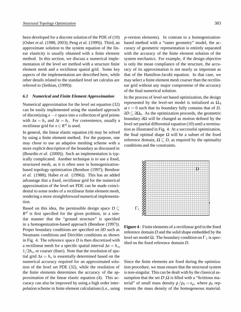
Based on this idea, the permissible design space D ⊆Rd is first specified for the given problem, in a sim-ilar manner that the “ground structure” is specifiedin a homogenization-based approach (Bendsoe (1997)).Proper boundary conditions are specified on ∂D such asNeumann conditions and Dirichlet conditions as shownin Fig. 4. The reference space D is then discretized witha rectilinear mesh for a specific spatial interval ∆x = hx,1/
2hx, or coarser (finer). Note that the resolution of spa-tial grid ∆x = hx is essentially determined based on thenumerical accuracy required for an approximated solu-tion of the level set PDE (32), while the resolution ofthe finite elements determines the accuracy of the ap-proximation of the linear elastic equation (4). This ac-curacy can also be improved by using a high order inter-polation scheme in finite element calculations (i.e., using
p-version elements). In contrast to a homogenization-based method with a “raster geometry” model, the ac-curacy of geometric representation is entirely separatedwith the accuracy of the finite element solution of thesystem mechanics. For example, if the design objectiveis only the mean compliance of the structure, the accu-racy of its approximation is not nearly as important asthat of the Hamilton-Jacobi equation. In that case, wemay select a finite element mesh coarser than the rectilin-ear grid without any major compromise of the accuracyof the final numerical solution.
In the process of level-set based optimization, the designrepresented by the level-set model is initialized as Ω 0
at t = 0 such that its boundary fully contains that of D,∂D ⊆ ∂Ω0. As the optimization proceeds, the geometricboundary ∂Ω will be changed as motion defined by thelevel-set partial differential equation (10) until a termina-tion as illustrated in Fig. 4. At a successful optimization,the final optimal shape Ω will be a subset of the fixedreference domain, Ω ⊆ D, as required by the optimalityconditions and the constraints.
f
D
Figure 4 : Finite elements of a rectilinear grid in the fixedreference domain D and the solid shape embedded by thelevel set model Ω. The boundary condition on Γ 1 is spec-ified on the fixed reference domain D.
Since the finite elements are fixed during the optimiza-tion procedure, we must ensure that the structural systemis non-singular. This can be dealt with by the classical as-sumption that the set D\Ω is filled with a “fictitious ma-terial” of small mass density ρ
/ρ0 = ερ, where ρ0 rep-
resents the mass density of the homogeneous material.
384 Copyright c© 2004 Tech Science Press CMES, vol.6, no.4, pp.373-395, 2004
Therefore,
ρ(Φ) = ρ0[(1−ερ
)H (Φ)+ερ] (33)
Further, in the numerical implementation, functions δ(Φ)and H(Φ) have to be approximated with a first order ac-curate, smoothed version such as defined in (Osher et al.(1988, 2001)). Thus, we define the following approxima-tion functions (Wang et al. (2003))
H(Φ) =
⎧⎪⎨⎪⎩
0 Φ < −ξ34
(Φξ − Φ3
3ξ3
)+ 1
2 −ξ ≤ Φ < ξ1 Φ ≥ ξ
δ(Φ) = dH (Φ)/
dΦ (34)
where ξ is a parameter of choice to determine the size ofthe bandwidth of numerical smoothing.
In this fashion, the geometric boundary of the structureunder optimization is always implicitly described as thezero level set of Φ (x, t) = 0. There is no need to explic-itly recover the boundary until the end of the optimiza-tion (Wang et al. (2003)). There exist many techniquesin most of the popular scientific software systems to com-pute iso-curves and iso-surfaces. For example, the well-known marching-cubes technique in computer graphicscan be directly applied to recover 2D and 3D level sets.
6.2 Discrete Computation Schemes
The discrete solution to the Hamilton-Jacobi equation(10) is computed using finite differences over discretetime steps ∆t = ht and on the discrete grid ∆x = hx overthe level set function. A highly robust and accurate com-putational method was developed by Osher and Sethian(1988) to address the problem of overshooting. Basedon the notion of weak solutions and entropy limits, a socalled “up-wind scheme” is proposed to solve (10) withthe following first order update equation
φn+1i jk
= φni jk −∆t
(max
((Vn)i jk ,0
)∇++min
((Vn)i jk ,0
)∇−
)(35)
where
∇+ = max(D−xi jk,0)2 +min(D+x
i jk,0)2
+max(D−yi jk,0)2 +min(D+y
i jk,0)2
+max(D−zi jk,0)2 +min(D+z
i jk,0)21/2,
∇− = max(D+xi jk,0)2 +min(D−x
i jk,0)2
+max(D+yi jk,0)2 +min(D−y
i jk,0)2
+max(D+zi jk,0)2 +min(D−z
i jk,0)21/2
and, ∆t is the time step, and D±xi jk,D
±yi jk and D±z
i jk are the re-spective forward (+) and backward (−) difference oper-ators on Φ n
i jk in the three dimensions of x ∈R3 separately.In addition, the time steps ∆t must be limited to ensurethe stability of the up-wind scheme (35). The Courant-Friedrichs-Lewy (CFL) condition requires ∆t to satisfy
∆t max∣∣∣(Vn)i jk
∣∣∣ ≤ ∆min ∆min = min(∆x,∆y,∆z) (36)
where ∆min stands for the minimum grid space among thethree spatial dimensions (Osher et al. (2003)).
Higher order schemes can also be obtained for thespace quantities ∇+ and ∇− for discrete approximation.They are typically constructed with an essentially non-oscillatory (ENO) interpolation as fully described in (Shuet al. (1988)). We have implemented this so-called “highresolution” scheme and fount that it is indeed more ac-curate than the first order scheme (Wang et al. (2003)).The first order time-explicit scheme (35) is well knownfor its numerical stability. It can be made of higher or-der through a total variation diminishing (TVD) Runge-Kutta scheme (Shu (1988)). As outlined in the literature(Sethian (1999); Shu (1988); Wang et al. (2003)), theseschemes are explicit schemes and hence can be imple-mented in a straightforward manner.
6.3 Local Schemes of Level Set Computation
While the up-wind scheme makes the level set methodnumerically robust, the level set equation can also bemade with its computational complexity proportional tothe boundary area of the structure being optimized ratherthan the size of the volume in which it is embedded. Thisis because the structural boundary is defined to be a sin-gle level set (at the zero level), thus the calculation ofsolutions over the entire range of the function Φ is un-necessary.
Structural Topology Optimization 385
An efficient method has been developed in (Peng et al.(1999)) by making the embedding function Φ as a dis-tance function. Then, while the function Φ is maintainedto be a signed distance function, a local computationof the level set requires update only those points whereΦ ≈ 0. This local computation scheme is simple and ef-ficient. It has been shown that this method has a formalcomplexity of O(N) in the 2D case and O(N 2) in the 3Dsolid case, where N is the size of the spatial grid in eachdirection of the level set (Peng et al. (1999)). In otherwords, the complexity of the level set model computa-tion remains at the level of its physical dimension, notof the higher dimension of its embedding function. Thisadvantage makes the local level set method practicallyattracting.
In this scheme we compute the signed distance functionas defined as the Eikonal equation
|∇Φ(x, t)|= 1 (37)
This gives rise to another PDE to solve for its steadystate,
∂Φ∂t
= sign(Φ)(1−|∇Φ|) (38)
where sign(Φ) = 2H (Φ)−1 is the signed distance func-tion (Osher et al. (1988)). This approach allows us toavoid finding the design boundary explicitly. Further-more, it also serves a purpose of re-initialization of thelevel set function Φ(x, t) in order to obtain highly accu-rate numerical results (Osher et al. (1988)). The solutionof this PDE would prevent Φ(x, t) from deviating awayfrom the signed distance function.
6.4 Velocity Extension and Smoothing
In the level set formulation, we need the normal velocityVn in a neighborhood of the design boundary or the zerolevel set Γ(t). As suggested in (Sethian (1999)), the mostnatural way to extend Vn off the design boundary is to letthe velocity Vn be constant along the normal to Γ(t) suchthat
∇Vn ·∇Φ = 0 (39)
This leads to the following hyperbolic partial differentialequation
∂Vn
∂t+ sign(Φ)
∇Φ|∇Φ| ·∇Vn = 0 (40)
Accurate and robust numerical schemes, such as the firstorder upwind method, exist to compute discrete solu-tions to partial differential equations of velocity exten-sion (Sethian (1999)). For simplicity of the presentation,the reader is referred to (Osher et al. (1988); Peng et al.(1999)) for detailed formulae.
As a notable advantage of the level set method, the struc-tural boundary is not tracked explicitly while the level setequation is solved over the rectilinear grids. Therefore,the velocity field defining the level set movement cannotbe directly evaluated for the boundary surface. We use asmoothing method to evaluate the velocity field over thefinite element nodes. We may introduce a general andpositive function with tight support as a weighting func-tion, such as the Gaussian function
α(x) =1√
2π∆mine−Φ2(x)
/∆2
min (41)
with a constant ∆min representing the minimal width ofthe along the level sets. The purpose is to use it to smooththe velocity vector Vn with an effect on the gradient of theobjective functional such that
minVn
∫D
(α (x)Vn (Φ)−Vn (u,w,Φ)δ(Φ)
)2dΩ (42)
By solving this least squares smoothing equation, we ob-tain a new non-local velocity field Vn (Φ) defined on therectilinear grid of computation.
7 Numerical Examples
Numerical examples are presented in this section formean compliance optimization problems that have beenwidely studied in the relevant literature (Bendsoe (1997);Bulman et al. (2001)). The objective function of theproblem is the strain energy of the structure with a mate-rial volume constraint,
J(u,Ω) =∫
DEε(u) : ε(u)dΩ (43)
For all examples, the material used is steel with a mod-ulus of elasticity of 200 GPa and a Poisson’s ratio of ν=0.3. For clarity in presentation, the examples are in 2Dunder plane stress condition.
7.1 MBB Beams
This example is known as MBB beams related to a prob-lem of designing a floor panel of a passenger airplane in
386 Copyright c© 2004 Tech Science Press CMES, vol.6, no.4, pp.373-395, 2004
(a)(b)
(c) (d)
(e) (f)
(g) (h)
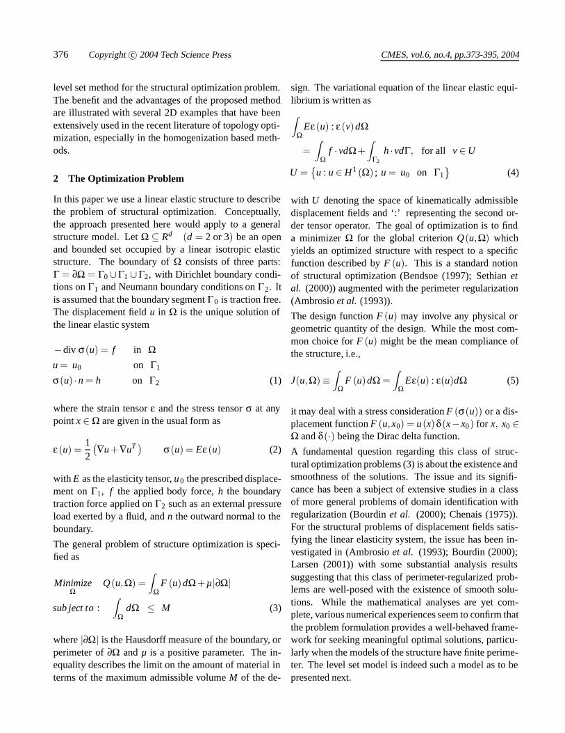
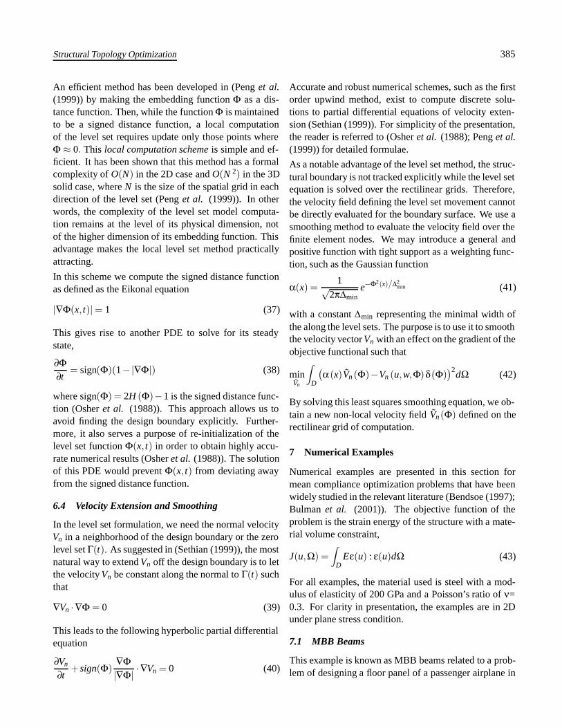
Figure 5 : A mid-point loaded MBB beam with fixed-simple supports and a volume ratio of 0.3. (a) Initial designof the right half. (b – g) Intermediate results. (h) Final solution.
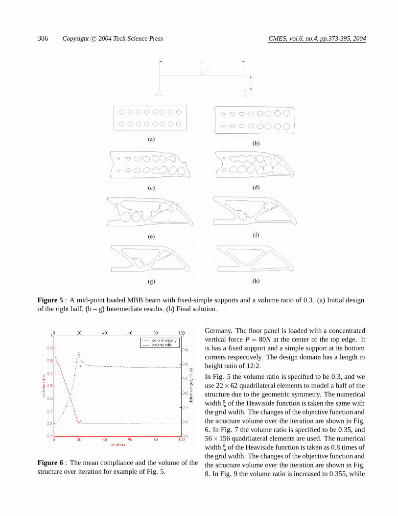
Figure 6 : The mean compliance and the volume of thestructure over iteration for example of Fig. 5.
Germany. The floor panel is loaded with a concentratedvertical force P = 80N at the center of the top edge. Itis has a fixed support and a simple support at its bottomcorners respectively. The design domain has a length toheight ratio of 12:2.
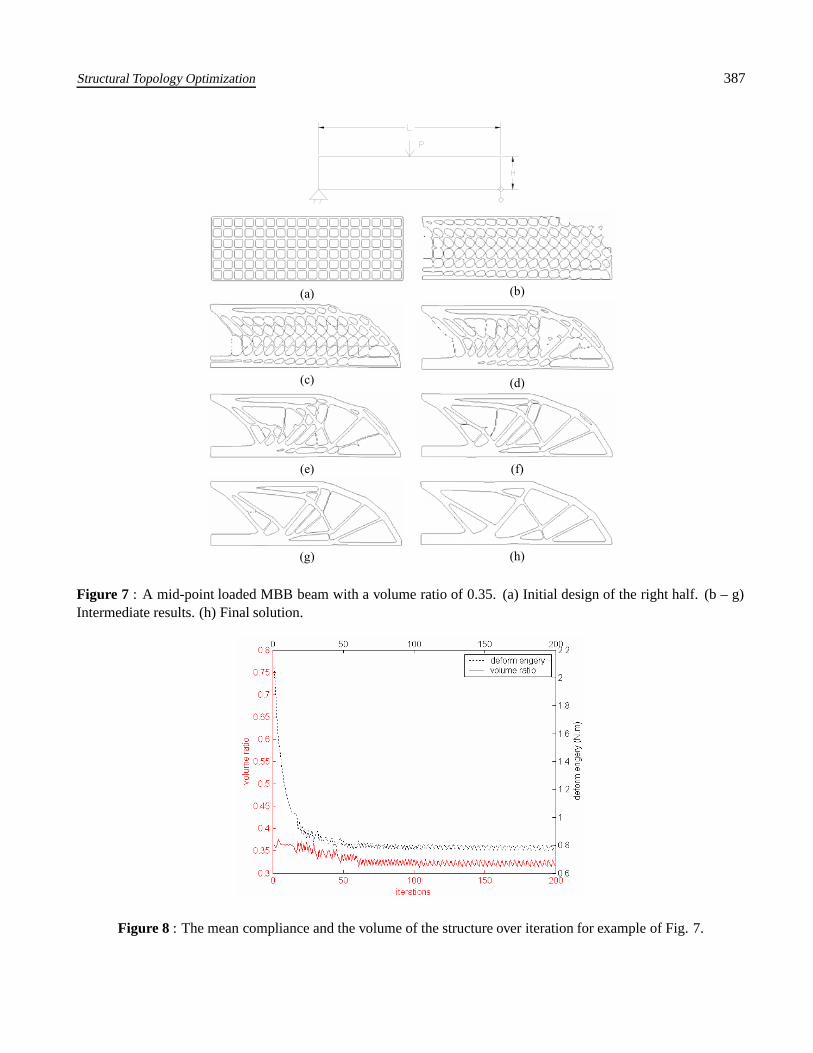
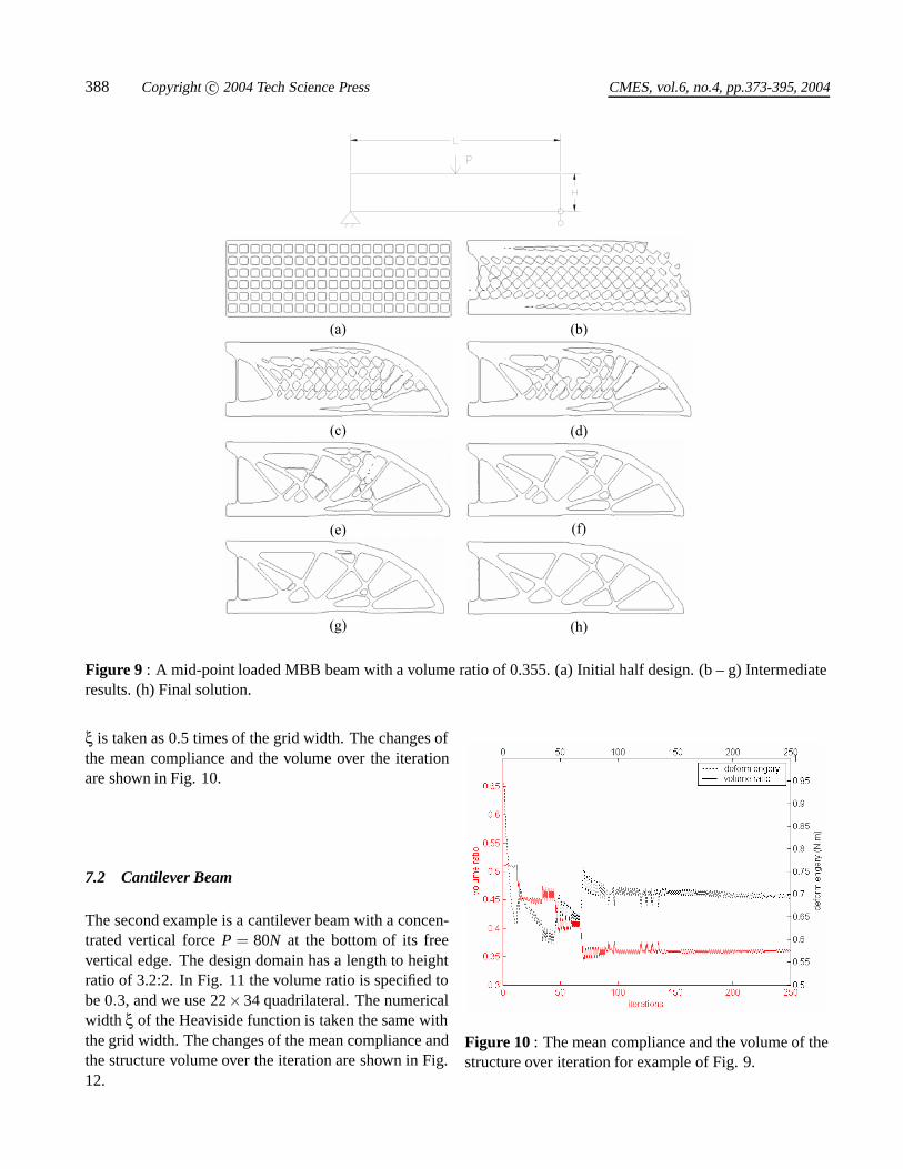
In Fig. 5 the volume ratio is specified to be 0.3, and weuse 22×62 quadrilateral elements to model a half of thestructure due to the geometric symmetry. The numericalwidth ξ of the Heaviside function is taken the same withthe grid width. The changes of the objective function andthe structure volume over the iteration are shown in Fig.6. In Fig. 7 the volume ratio is specified to be 0.35, and56×156 quadrilateral elements are used. The numericalwidth ξ of the Heaviside function is taken as 0.8 times ofthe grid width. The changes of the objective function andthe structure volume over the iteration are shown in Fig.8. In Fig. 9 the volume ratio is increased to 0.355, while
Structural Topology Optimization 387
(a) (b)
(c) (d)
(e) (f)
(g) (h)
Figure 7 : A mid-point loaded MBB beam with a volume ratio of 0.35. (a) Initial design of the right half. (b – g)Intermediate results. (h) Final solution.
Figure 8 : The mean compliance and the volume of the structure over iteration for example of Fig. 7.
388 Copyright c© 2004 Tech Science Press CMES, vol.6, no.4, pp.373-395, 2004
(a) (b)
(c) (d)
(e) (f)
(g) (h)
Figure 9 : A mid-point loaded MBB beam with a volume ratio of 0.355. (a) Initial half design. (b – g) Intermediateresults. (h) Final solution.
ξ is taken as 0.5 times of the grid width. The changes ofthe mean compliance and the volume over the iterationare shown in Fig. 10.
7.2 Cantilever Beam
The second example is a cantilever beam with a concen-trated vertical force P = 80N at the bottom of its freevertical edge. The design domain has a length to heightratio of 3.2:2. In Fig. 11 the volume ratio is specified tobe 0.3, and we use 22×34 quadrilateral. The numericalwidth ξ of the Heaviside function is taken the same withthe grid width. The changes of the mean compliance andthe structure volume over the iteration are shown in Fig.12.
Figure 10 : The mean compliance and the volume of thestructure over iteration for example of Fig. 9.
Structural Topology Optimization 389
(a) (b)
(c) (d)
(e) (f)
(g)(h)
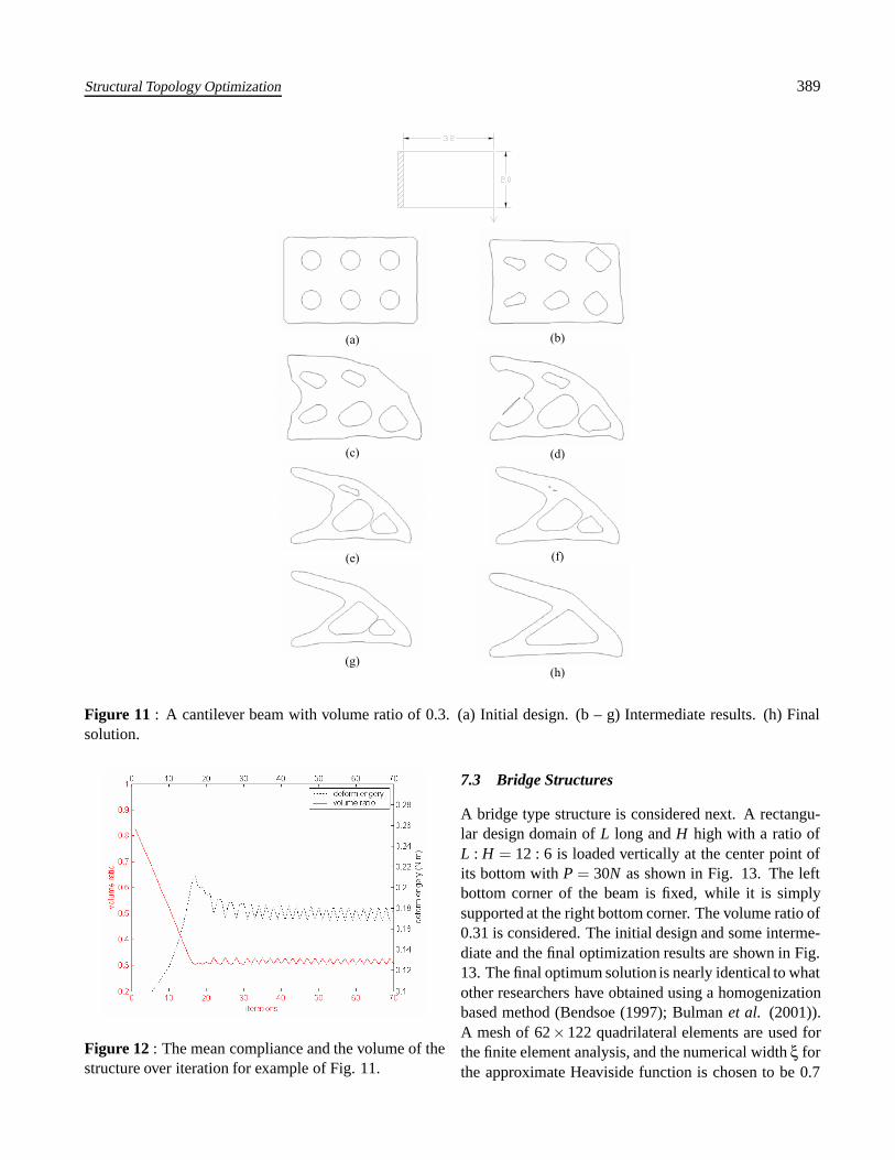
Figure 11 : A cantilever beam with volume ratio of 0.3. (a) Initial design. (b – g) Intermediate results. (h) Finalsolution.
Figure 12 : The mean compliance and the volume of thestructure over iteration for example of Fig. 11.
7.3 Bridge Structures
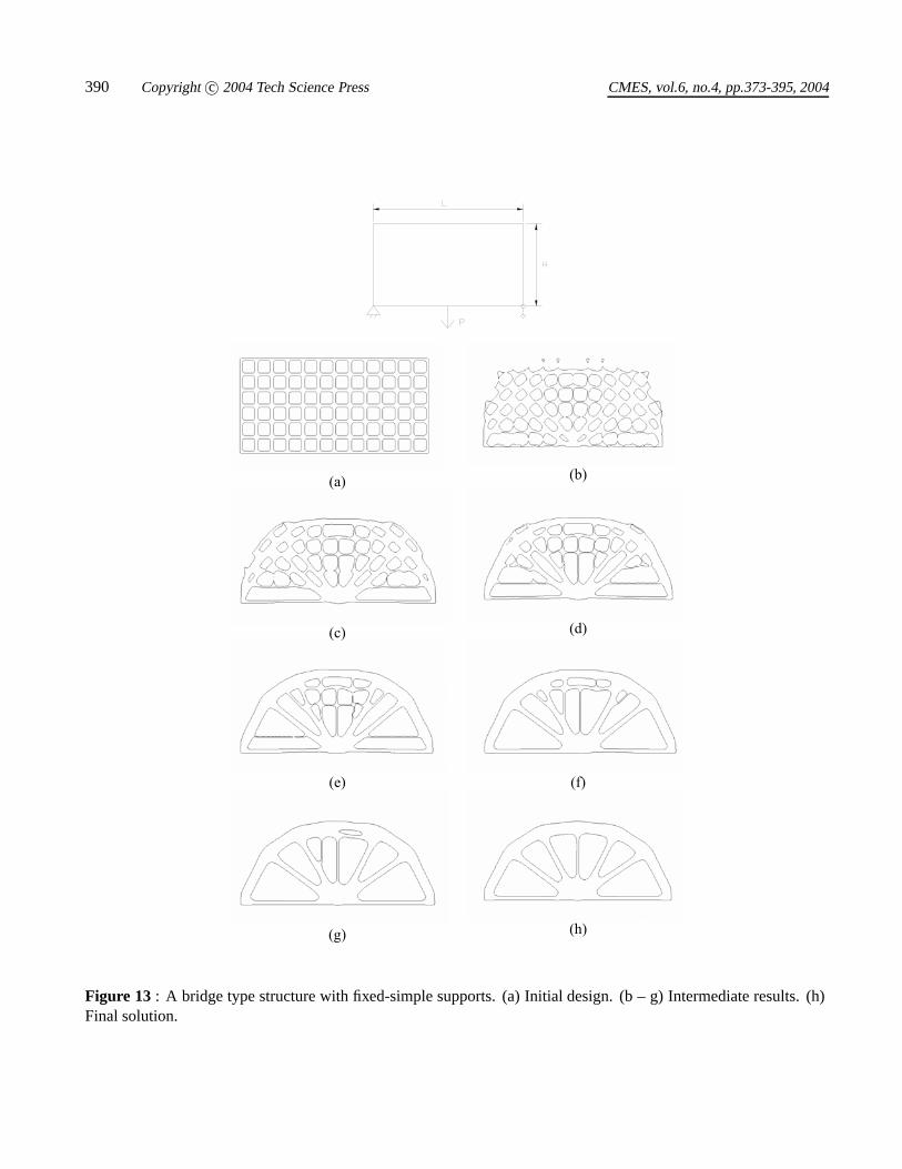
A bridge type structure is considered next. A rectangu-lar design domain of L long and H high with a ratio ofL : H = 12 : 6 is loaded vertically at the center point ofits bottom with P = 30N as shown in Fig. 13. The leftbottom corner of the beam is fixed, while it is simplysupported at the right bottom corner. The volume ratio of0.31 is considered. The initial design and some interme-diate and the final optimization results are shown in Fig.13. The final optimum solution is nearly identical to whatother researchers have obtained using a homogenizationbased method (Bendsoe (1997); Bulman et al. (2001)).A mesh of 62×122 quadrilateral elements are used forthe finite element analysis, and the numerical width ξ forthe approximate Heaviside function is chosen to be 0.7
390 Copyright c© 2004 Tech Science Press CMES, vol.6, no.4, pp.373-395, 2004
(a)(b)
(c) (d)
(e) (f)
(g) (h)
Figure 13 : A bridge type structure with fixed-simple supports. (a) Initial design. (b – g) Intermediate results. (h)Final solution.
Structural Topology Optimization 391
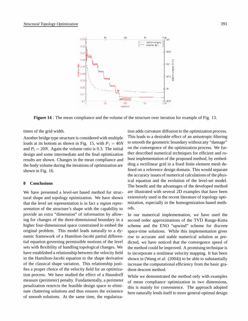
Figure 14 : The mean compliance and the volume of the structure over iteration for example of Fig. 13.
times of the grid width.
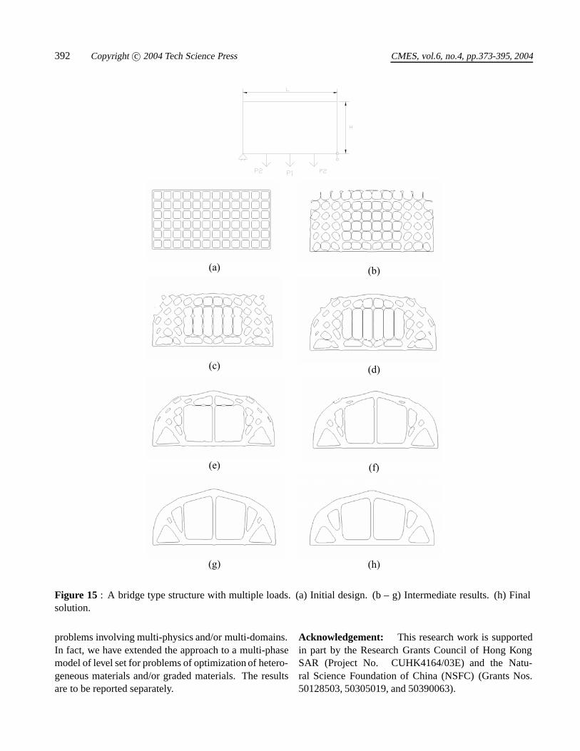
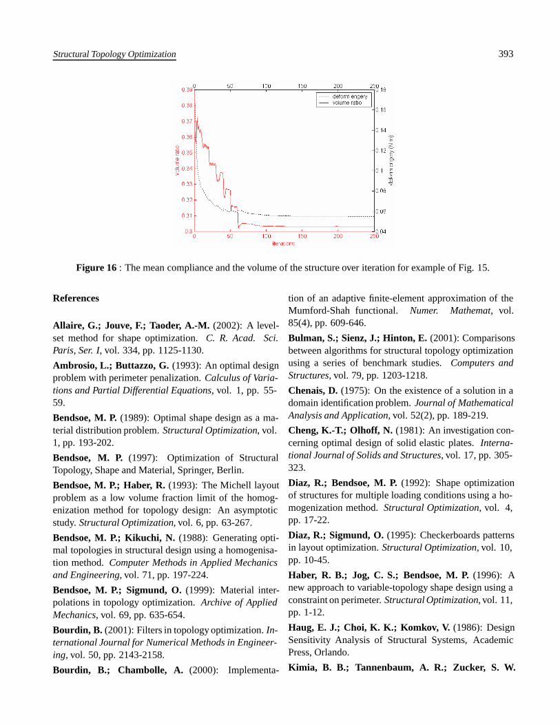
Another bridge type structure is considered with multipleloads at its bottom as shown in Fig. 15, with P1 = 40Nand P2 = 20N. Again the volume ratio is 0.3. The initialdesign and some intermediate and the final optimizationresults are shown. Changes in the mean compliance andthe body volume during the iterations of optimization areshown in Fig. 16.
8 Conclusions
We have presented a level-set based method for struc-tural shape and topology optimization. We have shownthat the level set representation is in fact a region repre-sentation of the structure’s shape with the capability toprovide an extra “dimension” of information by allow-ing for changes of the three-dimensional boundary in ahigher four-dimensional space constrained to embed theoriginal problem. This model leads naturally to a dy-namic framework of a Hamilton-Jacobi partial differen-tial equation governing permissible motions of the levelsets with flexibility of handling topological changes. Wehave established a relationship between the velocity fieldin the Hamilton-Jacobi equation to the shape derivativeof the classical shape variation. This relationship justi-fies a proper choice of the velocity field for an optimiza-tion process. We have studied the effect of a Hausdorffmeasure (perimeter) penalty. Fundamentally, a perimeterpenalization restricts the feasible design space to elimi-nate chattering solutions and thus ensures the existenceof smooth solutions. At the same time, the regulariza-
tion adds curvature diffusion to the optimization process.This leads to a desirable effect of an anisotropic filteringto smooth the geometric boundary without any “damage”on the convergence of the optimization process. We fur-ther described numerical techniques for efficient and ro-bust implementation of the proposed method, by embed-ding a rectilinear grid in a fixed finite element mesh de-fined on a reference design domain. This would separatethe accuracy issues of numerical calculations of the phys-ical equation and the evolution of the level-set model.The benefit and the advantages of the developed methodare illustrated with several 2D examples that have beenextensively used in the recent literature of topology opti-mization, especially in the homogenization based meth-ods.
In our numerical implementation, we have used thesecond order approximations of the TVD Runge-Kuttascheme and the ENO “upwind” scheme for discretespace-time solutions. While this implementation givesrise to accurate and stable numerical solution as pre-dicted, we have noticed that the convergence speed ofthe method could be improved. A promising technique isto incorporate a nonlinear velocity mapping. It has beenshown in (Wang et al. (2004)) to be able to substantiallyincrease the computational efficiency from the basic gra-dient descent method.
While we demonstrated the method only with examplesof mean compliance optimization in two dimensions,this is mainly for convenience. The approach adoptedhere naturally lends itself to more general optimal design
392 Copyright c© 2004 Tech Science Press CMES, vol.6, no.4, pp.373-395, 2004
(a) (b)
(c) (d)
(e) (f)
(g) (h)
Figure 15 : A bridge type structure with multiple loads. (a) Initial design. (b – g) Intermediate results. (h) Finalsolution.
problems involving multi-physics and/or multi-domains.In fact, we have extended the approach to a multi-phasemodel of level set for problems of optimization of hetero-geneous materials and/or graded materials. The resultsare to be reported separately.
Acknowledgement: This research work is supportedin part by the Research Grants Council of Hong KongSAR (Project No. CUHK4164/03E) and the Natu-ral Science Foundation of China (NSFC) (Grants Nos.50128503, 50305019, and 50390063).
Structural Topology Optimization 393
Figure 16 : The mean compliance and the volume of the structure over iteration for example of Fig. 15.
References
Allaire, G.; Jouve, F.; Taoder, A.-M. (2002): A level-set method for shape optimization. C. R. Acad. Sci.Paris, Ser. I, vol. 334, pp. 1125-1130.
Ambrosio, L.; Buttazzo, G. (1993): An optimal designproblem with perimeter penalization. Calculus of Varia-tions and Partial Differential Equations, vol. 1, pp. 55-59.
Bendsoe, M. P. (1989): Optimal shape design as a ma-terial distribution problem. Structural Optimization, vol.1, pp. 193-202.
Bendsoe, M. P. (1997): Optimization of StructuralTopology, Shape and Material, Springer, Berlin.
Bendsoe, M. P.; Haber, R. (1993): The Michell layoutproblem as a low volume fraction limit of the homog-enization method for topology design: An asymptoticstudy. Structural Optimization, vol. 6, pp. 63-267.
Bendsoe, M. P.; Kikuchi, N. (1988): Generating opti-mal topologies in structural design using a homogenisa-tion method. Computer Methods in Applied Mechanicsand Engineering, vol. 71, pp. 197-224.
Bendsoe, M. P.; Sigmund, O. (1999): Material inter-polations in topology optimization. Archive of AppliedMechanics, vol. 69, pp. 635-654.
Bourdin, B. (2001): Filters in topology optimization. In-ternational Journal for Numerical Methods in Engineer-ing, vol. 50, pp. 2143-2158.
Bourdin, B.; Chambolle, A. (2000): Implementa-
tion of an adaptive finite-element approximation of theMumford-Shah functional. Numer. Mathemat, vol.85(4), pp. 609-646.
Bulman, S.; Sienz, J.; Hinton, E. (2001): Comparisonsbetween algorithms for structural topology optimizationusing a series of benchmark studies. Computers andStructures, vol. 79, pp. 1203-1218.
Chenais, D. (1975): On the existence of a solution in adomain identification problem. Journal of MathematicalAnalysis and Application, vol. 52(2), pp. 189-219.
Cheng, K.-T.; Olhoff, N. (1981): An investigation con-cerning optimal design of solid elastic plates. Interna-tional Journal of Solids and Structures, vol. 17, pp. 305-323.
Diaz, R.; Bendsoe, M. P. (1992): Shape optimizationof structures for multiple loading conditions using a ho-mogenization method. Structural Optimization, vol. 4,pp. 17-22.
Diaz, R.; Sigmund, O. (1995): Checkerboards patternsin layout optimization. Structural Optimization, vol. 10,pp. 10-45.
Haber, R. B.; Jog, C. S.; Bendsoe, M. P. (1996): Anew approach to variable-topology shape design using aconstraint on perimeter. Structural Optimization, vol. 11,pp. 1-12.
Haug, E. J.; Choi, K. K.; Komkov, V. (1986): DesignSensitivity Analysis of Structural Systems, AcademicPress, Orlando.
Kimia, B. B.; Tannenbaum, A. R.; Zucker, S. W.
394 Copyright c© 2004 Tech Science Press CMES, vol.6, no.4, pp.373-395, 2004
(1995): Shape, shock, and deformations I: the compo-nents of two-dimensional shape and reaction-diffusionspace. International Journal of Computer Vision, vol.15, pp. 189-224.
Larsen, J. (2001): Regularity in two-dimensional vari-ational problems with perimeter penalties. C. R. Acad.Sci. Paris Ser. I Math., vol. 333(3), pp. 261-266.
Lin, C.Y.; Chao, L.-S. (1992): Automated image inter-pretation for integrated topology and shape optimization.Structural and Multidisciplinary Optimization, vol. 20,pp. 124-137.
Mlejnek, H. P. (1992): Some aspects of the genesis ofstructures. Structural Optimization, vol. 5, pp. 64-69.
Osher, S.; Sethian, J. A. (2003): Front propagatingwith curvature-dependent speed: Algorithms based onHamilton-Jacobi formulations. Journal of Computa-tional Physics, vol. 79, pp. 12-49.
Osher, S.; Fedkiw, R. (2003): Level Set Methods andDynamic Implicit Surfaces, Springer, New York.
Osher, S. J.; Santosa, F. (2001): Level set methodsfor optimization problems involving geometry and con-strains I. Frequencies of a two-density inhomogeneousdrum. Journal of Computational Physics, vol. 171, pp.272-288.
Peng, D. et al. (1999): A PED-based fast local level setmethod, Journal of Computational Physics, vol. 155, pp.410-438.
Petersson, J. (1999): Some convergence results inperimeter-controlled topology optimization. ComputerMethods in Applied Mechanics and Engineering, vol.171, pp. 123-140.
Petersson, J.; Sigmund, O. (1998): Slope constrainedtopology optimization, International Journal for Numer-ical Methods in Engineering, vol. 41, pp. 1417-1434.
Rozvany, G. (1988): Structural Design via OptimalityCriteria, Kluwer, Dordrecht.
Rozvany, G. (2001): Aims, scope, methods, history andunified terminology of computer aided topology opti-mization in structural mechanics. Structural and Mul-tidisciplinary Optimization, vol. 21, pp. 90-108.
Sapiro, G. (2001): Geometric Partial Differential Equa-tions and Image Analysis, Cambridge University Press,Cambridge.
Sethian, J. A.; Wiegmann, A. (2000): Structural bound-ary design via level set and immersed interface methods.
Journal of Computational Physics, vol. 163(2), pp. 489-528.
Sethian, J. A. (1999): Level Set Methods and FastMarching Methods: Evolving Interfaces in Computa-tional Geometry, Fluid Mechanics, Computer Vision, andMaterials Science, Cambridge University Press.
Sheen, D.; Seo, S.; Cho, J. (2003): A level set approachto optimal homogenized coefficients. CMES: ComputerModeling in Engineering & Sciences Vol. 4, No. 1, pp.21-30.
Shu, C.-W. (1988): Total-variation-diminishing timediscretization. SIAM J. Sci. Stat. Comput, vol. 9, pp.1073-1084.
Shu, C.-W.; Osher, S. (1988): Efficient implementationof essentially non-oscillatory shock capture schemes.Journal of Computational Physics, vol. 77, pp. 439-471.
Sigmund, O. (2000): Topology optimization: A tool forthe tailoring of structures and materials. Phil. Trans.:Math. Phys. Eng. Sci., vol. 358, pp. 211-228.
Sigmund, O. (2001): A 99 topology optimization codewritten in Matlab. Structural and Multidisciplinary Op-timization, vol. 21, pp. 120-718.
Sigmund, O.; Petersson, J. (1998): Numerical instabil-ities in topology optimization: a survey on proceduresdealing with checkerboards, mesh-dependencies and lo-cal minima, Structural Optimization, vol. 16(1), pp. 68-75.
Sokolowski, J.; Zolesio, J. P. (1992): Introductionto Shape Optimization: Shape Sensitivity Analysis,Springer-Verlag, New York.
Suzuki, K.; Kikuchi, N. (1991): A homogenizationmethod for shape and topology optimization. ComputerMethods in Applied Mechanics and Engineering, vol. 93,pp. 291-381.
Tapp, C.; Hansel, W.; Mittelstedt, C.; Becker, W.(2004): Weight-minimization of sandwich structures bya heuristic topology optimization algorithm. CMES:Computer Modeling in Engineering & Sciences, Vol. 5,No. 6, pp. 563-574.
Wang, M. Y.; Wang, X.; Guo, D. (2003): A level setmethod for structural topology optimization. ComputerMethods in Applied Mechanics and Engineering, vol.192(1-2), pp. 227-246.
Wang, M. Y.; Wang, X. (2004): “Color” level sets: Amulti-phase method for structural topology optimization
Structural Topology Optimization 395
with multiple materials. Computer Methods in AppliedMechanics and Engineering, vol. 193(6-8), pp. 469 –496.
Wang, X.; Wang, M. Y.; Guo, D. (2004): Structuralshape and topology optimization in a level-set frame-work of region representation. Structural and Multidis-ciplinary Optimization, vol. 27(1-2), pp. 1-19.
Wang, M. Y.; Zhou, S. (2004): Nonlinear diffusions instructural topology optimization. Structural and Multi-disciplinary Optimization, published online and in press.
Appendix A: Material and Shape Derivatives
We present a brief description of the material and shapederivatives relevant to the work discussed in the paperwith the following materials adapted from (Haug et al.(1986)):
Definition: For a given velocity vector V (x) in the shapetransformation (17), the material derivative u(x;V) ofu(x;V ) for x ∈ Ω is defined by
u(x;V ) = limt→0
1t[u(x+ tV )−u(x)]
Lemma 1: For a regular function f (x) defined on Ω,with an integral over Ω defined by
ψ1 =∫
Ωf (x)dΩ
the material derivative of ψ1 at Ω is given by
ψ′1 =
∫Ω
f ′ (x)dΩ+∫
Γf (x) (V ·n)dΓ
where Γ = ∂Ω and n is the unit normal to the infinitesimalarea dΓ.
Lemma 2: Consider an integral over Γ,
ψ2 =∫
Γg(x)dΓ
where g(x) is a regular scalar function defined on Γ.Then the material derivative of ψ2 at Ω is given by
ψ′2 =
∫Γ
g′ (x)dΓ+∫
Γ(∇g ·n+κg(x)) (V ·n)dΓ
where κ = div n = ∇ · n is the curvature of Γ in R2 andtwice the mean curvature of Γ in R3.
Lemma 3: Consider an integral over Γ,
ψ3 =∫
Γg(x) ·ndΓ
where g(x) is a regular vector function defined on Γ andn is the normal vector of Γ. Then the material derivativeof ψ3 at Ω is given by
ψ′3 =
∫Γ
(g′ (x) ·n+div g(x) (V ·n)
)dΓ