Embed Size (px)
Citation preview

PDE (Math 4163) Spring 2016
Some historical notes.
PDE arose in the context of the development of models in the physics ofcontinuous media, e.g. vibrating strings, elasticity, the Newtonian gravita-tional field of extended matter, electrostatics, fluid flows, and later bythe theories of heat conduction, electricity and magnetism. In addition,problems in differential geometry gave rise to nonlinear PDE’s such as theMonge˘ Ampe re equation and the minimal surface equations. The classi-cal calculus of variations in the form of the Euler-Lagrange principle gaverise to PDE’s and the Hamilton-Jacobi theory, which had arisen in mechan-ics, stimulated the analysis of first order PDE’s. During the 18th century,the foundations of the theory of a single first order PDE and its reductionto a system of ODE’s was carried through in a reasonably mature form.The classical PDE’s which serve as paradigms for the later developmentalso appeared first in the 18th and early 19th century. The one dimensionalwave equation
utt − c2uxx = 0 ,
was introduced and analyzed by d’Alembert in 1752 as a model of a vibrat-ing string. His work was extended by Euler (1759) and later by D. Bernoulli(1762) to 2 and 3 dimensional wave equations
utt − c2∆u = 0 ,
in the study of acoustic waves.
The Laplace equation
∆u = 0 ,
was first studied by Laplace in his work on gravitational potential fieldsaround 1780. The heat equation
ut − c2∆u = 0 ,
was introduced by Fourier in his celebrated memoir “The orie analytique dela chaleur” (1810-1822). Thus, the three major examples of second-orderPDE’s hyperbolic, elliptic and parabolic had been introduced by the firstdecade of the 19th century, though their central role in the classification ofPDE’s, and related boundary value problems, were not clearly formulateduntil later in the century. Besides the three classical examples, a profusion
1

of equations, associated with major physical phenomena, appeared in theperiod between 1750 and 1900:
The Euler equation of incompressible fluid flows, 1755.
The minimal surface equation by Lagrange in 1760 (the first major appli-cation of the Euler-Lagrange principle in PDE’s).
The Monge-Ampere equation by Monge in 1775.
The Laplace and Poisson equations, as applied to electric and magneticproblems, starting with Poisson in 1813, the book by Green in 1828 andGauss in 1839.
The Navier Stokes equations for fluid flows in 1822-1827 by Navier, followedby Poisson (1831) and Stokes (1845).
Linear elasticity, Navier (1821) and Cauchy (1822).
Maxwell’s equation in electromagnetic theory in 1864.
The Helmholtz equation and the eigenvalue problem for the Laplace oper-ator in connection with acoustics in 1860.
The Plateau problem (in the 1840’s) as a model for soap bubbles.
The Korteweg - De Vries equation (1896) as a model for solitary waterwaves.
(Adapted from
Haim Brezis, Felix Browder,
Partial Differential Equations in the 20th Century
Advances in Mathematics 135, 76-144 (1998).
Conservation laws on the real line
We begin the discussion of PDEs showing how some of theses can be ob-tained from basic physical conservation laws.
We consider a substance or other physical quantities like electrical chargedistributed over an interval (a, b) of the real line, during time interval (q, s) ,say, with the “space” variable denoted by x , and the “time“ variable de-noted by t ,
In order to be able to describe the situation mathematically, we make the
2

following basic assumptions.
(A1) Density:There is a (smooth) function u(x, t) defined on (a, b)× (q, s) , such that
Uα,β(t) =
∫ β
α
u(x, t)dx
is the amount of the quantity at time t in the interval (α, β) for all α, β .
The function u is called the density of the quantity.
(A2) Flux:
There is a smooth function φ(x, t) defined on (a, b)× (q, s) , such that
Φσ,τ (x) =
∫ τ
σ
φ(x, t)dt
is the amount of the quantity passing (in the direction of the) space variablethrough “a point” x ∈ (a, b) for any time interval (σ, τ); the function φ iscalled the flux of the quantity
(A3) Source (or Sink):There is a function f(x, t) on (a, b)× (q, s) , such that
Gα,β,σ,τ =
∫ τ
σ
∫ β
α
f(x, t) dxdt
the gain (or loss) of the quantity in (τ, σ)× (α, β) ; the function f is calledthe source function.
Now our experience relates those three quantities in the following manner:
The change
Uα,β(τ)− Uα,β(σ)
of the quantity in an interval (α, β) from a time t = σ to a time t = τ equals
Φσ,τ (α)− Φσ,τ (β)
the amount passed into (α, β) through x = α , minus the amount passedout of the interval at x = β,plus the amount Gα,β,σ,τ generated on (α, β) in the time interval (σ, τ)i.e.:
Uα,β(τ)− Uα,β(σ) =
Φσ,τ (α)− Φσ,τ (β) +Gα,β,σ,τ .
3
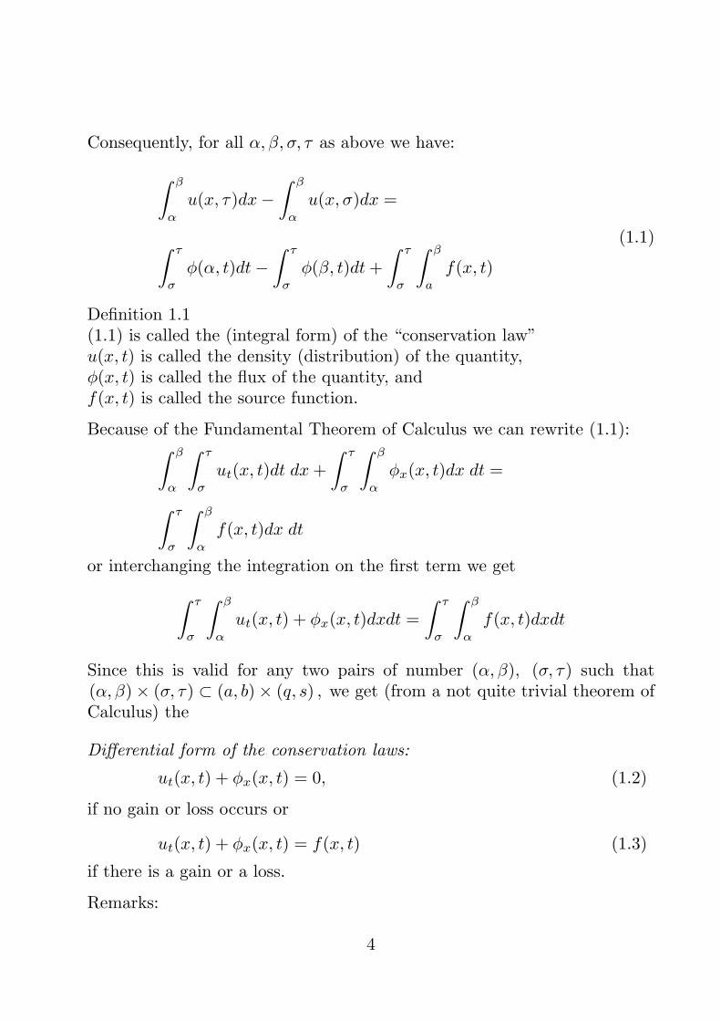
Consequently, for all α, β, σ, τ as above we have:
∫ β
α
u(x, τ)dx−∫ β
α
u(x, σ)dx =
(1.1)∫ τ
σ
φ(α, t)dt−∫ τ
σ
φ(β, t)dt+
∫ τ
σ
∫ β
a
f(x, t)
Definition 1.1(1.1) is called the (integral form) of the “conservation law”u(x, t) is called the density (distribution) of the quantity,φ(x, t) is called the flux of the quantity, andf(x, t) is called the source function.
Because of the Fundamental Theorem of Calculus we can rewrite (1.1):∫ β
α
∫ τ
σ
ut(x, t)dt dx+
∫ τ
σ
∫ β
α
φx(x, t)dx dt =
∫ τ
σ
∫ β
α
f(x, t)dx dt
or interchanging the integration on the first term we get
∫ τ
σ
∫ β
α
ut(x, t) + φx(x, t)dxdt =
∫ τ
σ
∫ β
α
f(x, t)dxdt
Since this is valid for any two pairs of number (α, β), (σ, τ) such that(α, β)× (σ, τ) ⊂ (a, b)× (q, s) , we get (from a not quite trivial theorem ofCalculus) the
Differential form of the conservation laws:
ut(x, t) + φx(x, t) = 0, (1.2)
if no gain or loss occurs or
ut(x, t) + φx(x, t) = f(x, t) (1.3)
if there is a gain or a loss.
Remarks:
4

1) These “laws” (1.1)-(1.3) are not proven in a mathematical sense, butconsequence from our basic assumption in order to use mathematics todescribe “real life” phenomena.
2) This law provides only one equation for the two unknown quantities u
and φ , so we need further information providing a relation betweenflux and the density to determine how the quantity evolves in time.Those may vary considerably with the particular situation under con-sideration. Usually, the resulting relations are called constitutive rela-tions, often provided in the form φ(x.t) = g(x, t, u, ux, ...).
Example:
Assume we have observed that a density function u(x, t) moves along a linewith a constant speed c , say, a signal along a wire. That is we have
u(x+ ch, t+ h) = u(x, t) ,
for (x, t) ∈ (−∞,∞)× (−∞,∞), and h in R .
On the other hand, we must have that∫ σ+h
σ
φ(α, t)dt ,
the amount of the quantity which passed through x = α in the time interval(σ, σ + h) equals
∫ α
α−ch
u(x, σ)dx ,
the amount of the quantity in the interval (α− ch, α) at time σ. So we get∫ σ+h
σ
φ(α, t)dt =
∫ α
α−ch
u(x, σ)dx (1.5)
If φ and u are continuous, then the mean value theorem provides∫ σ+h
σ
φ(α, t)dt = h · φ(α, s)
for some s , with σ < s < σ + h . and∫ α
α−ch
u(x, σ)dx = ch · u(ξ, σ)
for some ξ , with α− ch < ξ < α ,
5
Hence dividing (1.5) by h and letting h go to zero we find
cu(x, t) = φ(x, t) .
That is: the density is proportional to the flux, and for all(x, t) ∈ (−∞, ∞)× (−∞,∞) we get from (1.2):
ut + cux = 0.
Suppose now that we have obtained the information that for a certain quan-tity with density function u(x, t) on ((−∞,∞) × (−∞,∞) say) the flux isproportional to the density function. Can we conclude that the densityfunction is moving with constant speed?
In mathematical terms that is: Does a solution of
ut(x, t) + cux(x, t) = 0.
has the form
u(x, t) = u(x+ ch, t+ h) ?
Remark:
There are, of course, other constitutive relations. Such as φ = aux i.e.the flux is proportional to the slope of the distribution, as for the heat anddiffusion equations. We will be concerned with those later.
1. Linear First order PDE’s.
Definition:The equation.
aux + buy + du = g ,
for R = (x, y) ∈ (α, β)× (γ, δ) ,
with a, b, d, g (continuous) functions on R is called a linear first order PDEon R .
If g ≡ 0 then the equation is called homogeneous.
Equations of the form
aux + buy = 0 , (1.6)
Recall: Directional derivatives:
6

In calculus we have defined
fv(w) = (∂
∂vf)(w) = lim
h→0
1
h(f(w + hv)− f(w))
to be the derivative of f at w in the direction of v. Here f is a real valuedfunction defined, say, on D an open subset Rn, w ∈ D and v is any vectorin Rn.
Examples:
The partial derivatives are directional derivatives in the direction of thebasis vectors of the standard basis in Rn, i.e.:
fek=
∂
∂ekf =
∂
∂xkf = fxk
In general we have
fv = v · ∇f =∑
i=1
n
vi∂
∂xif
for functions
f = f(x1, . . . , xn) and vectors v = (v1, . . . , vn) .
In our case we get from (1.6) for v = (a, b) and u = u(x, y) that
0 = aux + buy = v · ∇u = uv
i..e.: if we are moving along a line with direction vector v then the derivativeof u in this direction is zero, hence there is no change along this line. Inother words u(x, y) is constant along lines of direction v.
Next we recall that any point r = (x, y) on a line L satisfies the equation
r = r0 + tv
for some fixed point r0 = (x0, y0) on that line and with direction vectorv = (a, b).
Since n · v = 0 for n = (b,−a) we find:
0 = n · (r − r0) = bx− ay − b · x0 + ay0 ,
or
bx− ay = c , (1.7)
for some constant c = bx0 − ay0.
7

The above observation includes that for each real number c we have a linegiven by (1.7) along which the solution u is constant, say f(c), i.e., thesolution u defines a function f : c → f(c) and we have
u(x, y) = f(c) , if (bx− ay) = c.
Hence a solution of (1.6) ( if there is one) has to be of the form,
u(x, y) = f(bx− ay) .
On the other hand, if f is differentiable we get
ux(x, y) =d
dx(f(bx− ay)) = f ′(bx− ay)b
and
uy(x, y) =d
dy(f(bx− ay)) = −f ′(bx− ay)a
and so
(aux − buy)(x, y) = (ab− ba)(f ′(bx− ay)) = 0 .
We found indeed a solutions of (1.6) .
Initial value problems:
With the fact that u(x, y) = f(bx − ay) we have used all the informationprovided by the PDE. We have to infer auxiliary condition to determined thesolution uniquely. The most important one is the so called initial condition:
Suppose that u(x, y) satisfies the PDE above and we know the function ofu is g(x) at a certain line, y = 0, say. Then we must solve
(IV P )
{
aux + buy = 0u(x, 0) = g(x)
This is called an initial value problem (IVP).
We know, the solutions must be of the form
u(x, y) = f(bx− ay)
implying
g(x) = u(x, 0) = f(bx− 0) = f(bx) .
8
We know the function g by assumption and want to determine f .
Setting r = bx we solve for x and get
x =r
b.
That is, the function f must be given by
f(r) = g(1
br) ,
writing r for the independent variable. Hence for the solution we get
u(x, y) = f(bx− ay) = g(1
b(bx− ay)) ,
So
u(x, y) = g(x− a
by) ,
is a solution of the (IVP).As shown earlier it solves the PDE and we have
u(x, 0) = g(x) .
Change of variables
A slightly different approach is to introduce “characteristic” variables:
First we consider equation of the form
a(x, y)ux + b(x, y)uy = 0
We introduce the new coordinate system{
ξ = s(x, y)η = y
where s(x, y) = c is an implicit solution of the ODE
y′(x) =b(x, y)
a(x, y),
or more generally an implicit solution of the ODE
a(x, y)dy = b(x, y)dx .
That later equation showing clearly that it is equivalent to think of thosecurves as functions in x or functions in y .
9

To motivate that choice of coordinate system, we consider u(x, y) along agraph given by the solution y(x) of the above ODE. Then we have
d
dxu(x, y(x)) = ux + uyy
′ = 0 ,
and so
a(x, y)ux + b(x, y)uy = 0
Hence the solution does not change along the integral curves of the ODE.The curves defined by the equations s(x, y) = c are called the characteristicsof the PDE.Note, differentiating s(x, y(x)) = c , with respect to x we get
asx + bsy = 0 , orsx(x, y)
sy(x, y)= − b(x, y)
a(x, y).
For the second variable η we can chose any linear combination of x and y ,
as long as that is not colinear with ξ in an open subset of the plane.
Now, with the above change of variables, we get a function U = U(ξ, η) bysetting
U(ξ, η)ξ=s(x,y)
η=y
= u(x, y) .
So u(x, y) = U(s(x, y), y)and we have
ux = Uξsx and uy = Uξsy + Uη .
From the PDE we obtian the equation
0 = aUξsx + b(Uξsy + Uη) = (asx + bsy)Uξ + bUη = bUη .
or
Uη = 0 .
That is U has to be constant in η , so it can vary only in ξ , and we musthave
U(ξ, η) = G(ξ)
for some function G , providing
u(x, y) = G(s(x, y)) .
10
Again G has to be determined by auxiliary conditions.
Example:
Consider
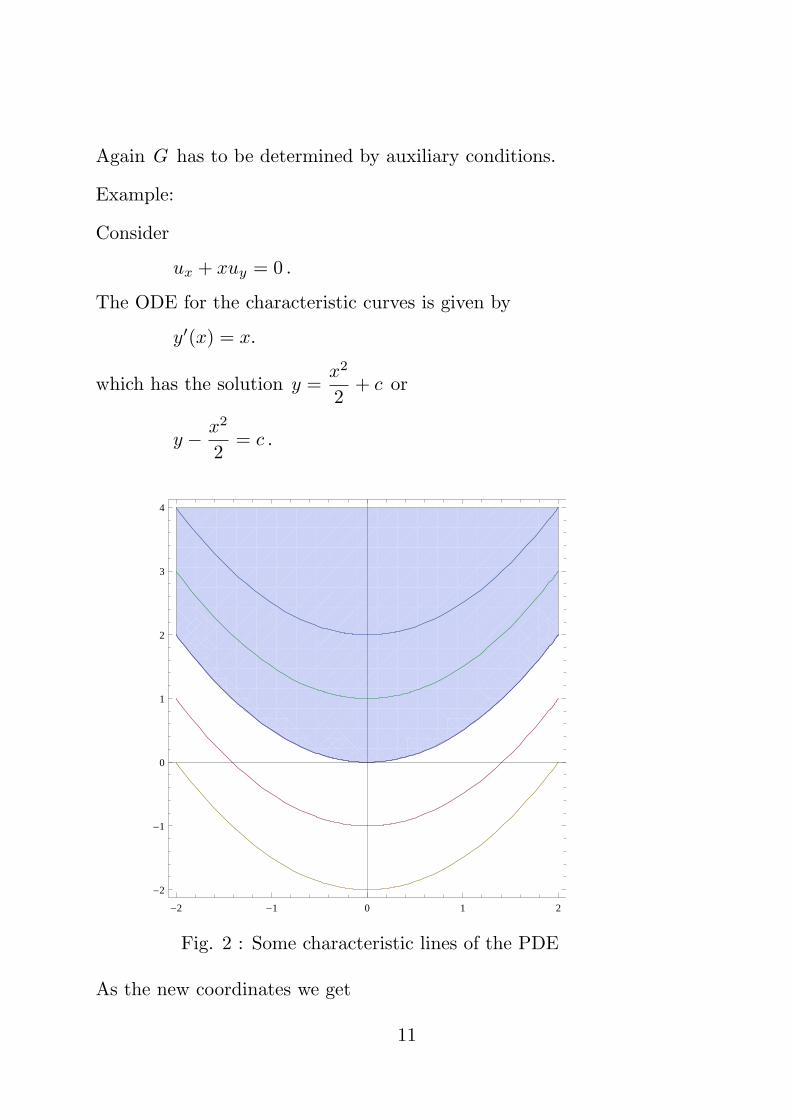
ux + xuy = 0 .
The ODE for the characteristic curves is given by
y′(x) = x.
which has the solution y =x2
2+ c or
y − x2
2= c .
-2 -1 0 1 2
-2
-1
0
1
2
3
4
Fig. 2 : Some characteristic lines of the PDE
As the new coordinates we get
11

{
ξ = y − x2
2,
η = y
So introducing the function U = U(ξ, η) such that
U(ξ, η)ξ=y− x2
2
η=y
= u(x, y) ,
we get
ux = −Uξ x and uy = Uξ + Uη ;
Because of the PDE we must have
Uη = 0 i.e: U(ξ, η) = G(ξ)
Consequently the general solution of the PDE is
u(x, y) = G(y − x2
2) .
Now consider the auxiliary condition
u(x, 0) = g(x) .
It provides
g(x) = u(x, 0) = G(−x2
2) .
To find G as a function of a real variable, r say, we set r = −x2
2and solve
for x . This gives
x =√−2r .
So the function G(r) = g(√−2r) and the solution of the initial value prob-
lem is
u(x, y) = g(
√
−2(y − x2
2) ) = g(
√
x2 − 2y) .
Note that u(x, y) = g(√
x2 − 2y) is defined for all (x, y) for which 2y ≤ x2 .
Since for negative x we have x = −√x2 we need g(x) = g(−x) in order
for that initial value problem to have a solution at all.
Also, for the region in the plane for which 2y > x2 , that is the area (shaded
12
in Fig. 2) above the parabola through the origin, the solution is not deter-mined by g at all.
Apparently the auxiliary condition cannot be chosen freely on just anycurve. Note, the line given by y = 0 is parallel to the tangent of thecharacteristic through the origin at that very point.
We say the problem is “well posed” if the auxiliary condition(s) provide theexistence of a unique solution in the domain in which we consider the PDE.The above example indicates that possibly problems are not well posed ifthe auxiliary conditions are given on curves which are characteristic at somepoints i.e.: the auxiliary condition are chosen on curves which are tangentto a characteristic curve at some points.
The line given by x = 0 is nowhere tangent to characteristics and we obtaina unique solution for
(∗){
ux + xuy = 0u(0, y) = φ(y)
.
Indeed we must have
φ(y) = u(0, y) = G(y − x2
2)x=0
= G(y) .
So the solution has to be of the form u(x, t) = φ(y − x2
2) and it is straight
forward to check that it is indeed a solution of (∗) .
Exmaple 2
For constant coefficients,
aux + buy = 0 ,
the ODE for the characterstics is
y′ =b
a,
which has the solutions y =b
ax + d, foe some constant d . Since a is
constant we get equivalently
ay − bx = c , with c = da .
Setting
13
{
ξ = ay − bx ,
η = y
we define the function U by
U(ξ, η)ξ=ay−bx
η=y
= u(x, y)
i.e.:
u(x, y) = U(ay − bx, y)
Note: that in the new variables U does not vary if we keep ξ , constant. Sono matter would linear combination of x and y we choose for the secondvariable η , such that ξ and η are linearly independent,the solution doesnot change if ξ is fixed and η changes. We always will have Uη = 0 .
Indeed we get
ux = −bUξ and uy = aUξ + Uη ;
or
0 = aux + buy = −abUξ + baUξ + bUη
and for b 6= 0 , (otherwise ξ and η would be linearly independent.
Uη = 0 .
Hence
U = C(ξ) i.e.: u(x, y) = C(ay − bx) .
For u = u(x, t) and the equation
ut + cux = 0 ,
we have a = c and b = 1 so ξ = t− x
c, η = t and the general solution
u(x, t) = C(ct− x) = C̃(x− ct) .
Back to our problem: does the solution of
ut + cux = 0 ,
model a fixed shape moving along a line with constant speed?
14

As a solution of the PDE u(x, t) must be of the form u(x, t) = f(x − ct).Does this describe a density moving to the right? Let’s see:
u(x+ ch, t+ h) = f(x+ ch− c(t+ h)) =
f(x− ct) = u(x, t).
Yes, it does.
Note: The argument of u is a point, (vector) in R2, where as the argumentof f is a real number!
Example:
g(x) =
{
cosx ,π
2≤ x ≤ π
2;
0 , otherwise ;
then
u(x, t) =
{
cos(x− ct) ,π
2≤ x− ct ≤ π
2;
0 , otherwise .
Fig. 1 : Solution of the IPV
There are many curves along which we can prescribe the values for u , for
15

instance consider
(IV P )
{
ut + cux = 0u(0, t) = φ(t)
then we must have
φ(t) = u(0, t) = f(−ct) .
With τ = −ct we get t = −τ
c, and f(τ) = φ(−τ
c) , providing the solution,
u(x, t) = φ(t− x
c) .
1.2 Linear equation with non-constant coefficients:
We consider equation of the form
a(x, y)ux + b(x, y)uy + d(x, y)u = f(x, y)
and again introduce the new coordinate system{
ξ = s(x, y)η = y
where s(x, y) = c is a implicit solution of the ODE.
y′(x) =b(x, y)
a(x, y),
For U = U(ξ, η)U(ξ, η)
ξ=s(x,y)
η=y
= u(x, y) .
i.e.: u(x, y) = U(s(x, y), y)we have
ux = Uξsx and uy = Uξsy + Uη .
and obtain from the PDE the equation
b(x, y)Uη(ξ, η))ξ=s(x,y)
η=y
+ d(x, y)u = f(x, y) .
With D(ξ, η) and F(ξ, η) given by
16
D(ξ, η)ξ=s(x,y)
η=y
=d(x, y)
b(x, y)and F(ξ, η)
ξ=s(x,y)
η=y
=f(x, y)
b(x, y),
respectively, we find that U is subject to the linear ODE
Uη +DU = F ,
in η , (for fixed ξ .) For fixed ξ the (general) solution are determined up toa constant C , which may depend on ξ , i.e.: the solution is of the form
U(ξ, η) = w(η, ξ) + C(ξ)h(η, ξ) .
and we determine C(ξ) using the auxiliary condition, where w(η, ξ) is onesolution of the inhomogeneous ODE
Uη +D(ξ, η)U = F (ξ, η) ,
and h(η, ξ) is a solution of the homogeneous ODE
Uη +D(ξ, η)U = 0 ,
in η for fixed ξ . The dependence of h,w and C on ξ is then determinedwith the help of th auxiliary condition.
Recall: The general formular for the solution of a linear first order ODE
y′ + P (x)y = Q(x) ,
is given by
y = e−
∫
P (x)dx(
∫
Q(x)e∫
P (x)dxdx+ C) ;
Also recall that the integrating factor is given by
ρ(x) = exp(
∫
P (x))dx .
Example 1
For the general initial boundary value problem with constant coefficients{
aux + buy + du = g, ,
u(x, 0) = h(x) .,
we get
y′ =b
a,
17
so s(x, y) = ay − bx , and we have to solve the ODE
Uη +d
bU =
g
b,
which has the soltion
U = C(ξ)e−dbη +
g
d,
and we get the general solution
u(x, y) = C(ay − bx)e−dby +
g
d.
The initial condition provides
h(x) = u(x, 0) = C(−bx) + +g
d.
With r = −bx , and x = −r
b, we find
C(r) = h(−r
b)− g
d,
which yields the solution
u(x, y) = (h(x− a
by)− g
d)e−
dby +
g
d.
Example 2:{
xux + yuy + yu = x ,
u(x, 1) = g(x) .
First lets find the general solution of the PDE:
The ODE for the characteristics is given by
y′(x) =y
x.
which is a separable ODE with the solution y = c̃x or
c̃ =y
xor equivalently c =
x
y.
18

-2 -1 1 2
-2
-1.5
-1
-0.5
0.5
1
1.5
2
Fig. 3 : Some characteristic lines of the PDE
As the new coordinates we get
ξ =x
y,
η = y
So for
U(ξ, η)ξ= x
y
η=y
= u(x, y)
We get
ux = Uξ1
yand uy = −Uξ
x
y2+ Uη ;
Because of the PDE we must have
yUηξ= x
y
η=y
+ yu = x ,
or
19
Uη + U = ξ ,
which has the solution:
U(ξ, η) = ξ + C(ξ)e−η .
Consequently the general solution of the PDE is
u(x, y) = (x
y) + C(
x
y)e−y .
The initial condition provides
g(x) = u(x, 1) = x+ C(x)e−1 .
With r = x, we get
C(r) = e · (g(r)− r) ,
and so the solution of the problem is
u(x, y) =x
y+ e1−y(g(
1
x)− x
y) .
Example 3:
{
ux + y2uy + u = x+1
y,
u(x, 0) = g(x)(?) .
First lets find the general solution of
ux + y2uy + u = x+1
y.
The ODE for the characteristics is given by
y′(x) = y2.
which is a separable ODE with the solution −1
y= x+ c or y =
1
c− x.
20

-3 -2 -1 1 2 3
-2
-1.5
-1
-0.5
0.5
1
1.5
2
c = 0 c > 0
c < 0 c = 0
Fig. 4 : Some characteristic lines of the PDE
Note that the sketch shows, that the initial value problem is ill posed.
As the new coordinates we get{
ξ = x+1
y,
η = y
So for
U(ξ, η)ξ=x+ 1
y
η=y
= u(x, y)
We get
ux = Uξ and uy = −Uξ1
y2+ Uη .
Because of the PDE and x = ξ − 1
ηwe must have
Uη +1
η2U =
1
η2ξ .
That is a linear first oder ODE which has the solution
U = ξ + C(ξ)e1/η .
(Integrating factor (exp(
∫
pdη) , p =1
η2. )
Consequently the general solution of the PDE is
21

u(x, y) = x+1
y+ C(x+
1
y)e1/y . (∗)
Since the problem as intended is ill posed, let us consider two other auxiliaryconditions u(x, 1) = g(x) , and u(0, y) = f(y) .
For u(x, 1) = g(x) , we have
g(x) = u(x, 1) = x+ 1 + C(x+ 1)e ,
With r = x+ 1 and x = r − 1 this implies
C(r) =−r + g(r − 1)
e.
and so inserting the argument x+1
yin C we get the soltion
u(x, y) = x+1
y+ (−(x+
1
y) + g(x+
1
y− 1))e
1
y−1
The second auxiliary condition f(y) = u(0, y) provides
f(y) = u(0, y) =1
y+ C(
1
y)e1/y ,
With r =1
yand y =
1
rthis implies
C(r) =−r + f(
1
r)
er.
Again we have to replace r by the argument of C in (*) that is x+1
y, and
we get
u(x, y) = x+1
y+ (f(
y
xy + 1)− x− 1
y)e−x .
22