A&A 594, A90 (2016)DOI: 10.1051/0004-6361/201527612c© ESO 2016

Astronomy&Astrophysics

Transient effects in Herschel/PACS spectroscopyDario Fadda1,2,?, Jeffery D. Jacobson3, and Philip N. Appleton3

1 Instituto de Astrofisica de Canarias, 38205 La Laguna, Tenerife, Spaine-mail: darioflute@gmail.com

2 Universidad de La Laguna, Dpto. de Astrofísica, 38206 La Laguna, Tenerife, Spain3 NASA Herschel Science Center – California Institute of Technology, MC 100-22, Pasadena, CA 91125, USA

e-mail: [jdj;apple]@ipac.caltech.edu

Received 21 October 2015 / Accepted 18 January 2016

ABSTRACT

Context. The Ge:Ga detectors used in the PACS spectrograph onboard the Herschel space telescope react to changes of the incidentflux with a certain delay. This generates transient effects on the resulting signal which can be important and last for up to an hour.Aims. The paper presents a study of the effects of transients on the detected signal and proposes methods to mitigate them especiallyin the case of the unchopped mode.Methods. Since transients can arise from a variety of causes, we classified them in three main categories: transients caused by suddenvariations of the continuum due to the observational mode used; transients caused by cosmic ray impacts on the detectors; transientscaused by a continuous smooth variation of the continuum during a wavelength scan. We propose a method to disentangle these effectsand treat them separately. In particular, we show that a linear combination of three exponential functions is needed to fit the responsevariation of the detectors during a transient. An algorithm to detect, fit, and correct transient effects is presented.Results. The solution proposed to correct the signal for the effects of transients substantially improves the quality of the final reductionwith respect to the standard methods used for archival reduction in the cases where transient effects are most pronounced.Conclusions. The programs developed to implement the corrections are offered through two new interactive data reduction pipelinesin the latest releases of the Herschel Interactive Processing Environment.

Key words. methods: data analysis – techniques: spectroscopic – infrared: general

1. Introduction

The Herschel Space Observatory (Pilbratt et al. 2010) completedits mission on April 29, 2013 after performing a total of 23 400 hof scientific observations during almost 4 years of activity (1446operational days). One of the most used instruments aboardHerschel was the PACS spectrometer (Poglitsch et al. 2010). Ap-proximately one quarter of the total scientific time was devotedto PACS spectroscopy. Although most of the observations wereperformed in the standard chop-nod mode, a substantial frac-tion (30% of the observations, corresponding to the 25% of thetotal spectroscopy time) used two alternative modes. The wave-length switching mode was released to users after the start of themission to allow PACS spectrometer observations to be made incrowded fields where chopping was not possible. A year later,this mode was replaced by the so-called unchopped mode. Bythe end of the Herschel operation mission, this mode was usedfor approximately one-third of all PACS spectroscopic observa-tions. The primary focus of this paper is to describe an optimalway to reduce data taken in the unchopped mode.

The PACS spectrometer was able to observe spectroscopi-cally between 60 µm and 210 µm using Ge:Ga photo-conductorarrays. This type of detectors suffers from systematic mem-ory effects of the response which can bias the photometry ofsources and increase the noise in the signal. Such effects havebeen documented and studied for similar detectors on previousspace observatories such as ISOCAM (Coulais & Abergel 2000;Lari et al. 2001) and MIPS (Fadda et al. 2006, Fig. 17).

? Moving to the SOFIA Science Center (USRA).

In this paper we briefly review the observational modesof the PACS spectrograph and the data reduction techniques.We describe how the unchopped mode is particularly sensitiveto sudden changes in incident flux, and cosmic ray glitches,which cause memory effects in the detector responses. Finally,we introduce the technique used to correct most of these ef-fects, and show a few selected examples. The methods andsoftware described in the paper are now implemented in theHerschel Interactive Processing Environment (HIPE1; Ott 2010).The comparisons presented in the paper are between the archivedSPG (standard product generation) products, generated withHIPE 14.0 and calibration data version 72, and our pipeline inHIPE 15.

2. The PACS spectrometer

We recommend reading Poglitsch et al. (2010) and the PACS ob-servational manual for a detailed description of the PACS spec-trometer. As a way to introduce some terminology used in thepaper, we give here a concise description of the instrument andhow it works.

The PACS spectrometer was an IFU (integral field unit) com-posed by a matrix of 5 × 5 spatial pixels (spaxels or spacemodules) covering a field of 47′ × 47′ square arcminutes. The5 × 5 pixel image passed into an image slicer, which rearrangedthe 5 × 5 two-dimensional image into one-dimension (1 × 25),which then fed a Littrow-mounted diffraction grating where it

1 www.cosmos.esa.int/web/herschel/hipe-download

Article published by EDP Sciences A90, page 1 of 14

A&A 594, A90 (2016)

operated at 1s, 2nd, and 3rd order. The first order (red) andsecond or third order (blue) were separated with a dichroicbeam-splitter, where the spectra were re-imaged onto separatedetectors. The wavelength range covered is 51–105 µm for theblue (choice of 51–73 and 71–105 µm for the 3rd and 2nd order)and 102–220 µm for the red, respectively.

The dispersed light was detected by two (low and high-stressed) Ge:Ga photo-conductors arrays with 25 × 16 pixels. Inthe following we call spectral pixels the individual pixels of thetwo arrays. We call module or spaxel (from spatial pixel) the setof 16 spectral pixels corresponding to the dispersed light from asingle patch of 9.4 × 9.4 square arcseconds on the sky.

Since the instantaneous wavelength range covered by16 spectral pixels is small (∼1500 km s−1 for many observa-tions), the grating was typically stepped through a range of grat-ing angles during an observation. This operation is referred asa wavelength scan. During a standard observation, the desiredwavelength range is covered by moving the grating back andforth. These movements are called up- and down-scans, sincethe wavelength seen by a single spectral pixel first increases andthen decreases as the grating executes a scan first in one direc-tion, and then back.

The other mobile part of the system is the chopper which liesat the entrance to the whole PACS instrument. This is a mirrorwhich allows the IFU to point at different parts of the sky. Instandard chop-nod mode, the chopping mirror is used to alter-natively point rapidly to the source and then a background posi-tion, while maintaining the same telescope pointing. The largestchopper throw available is 6 arcmin, which is a limitation of thechop-nod mode. If the chopper mirror is moved to larger angles,it can access two internal calibrators (BB1 and BB2) which areused for calibration during the slew to the target source.

Since the mirror is passively cooled, the emission of the tele-scope is significant, and typically dominates the total signal. Forinstance, in the red, the emission seen by a given pixel at 120 µmis around 300 Jy. This high telescope background level, althoughnot generally desirable in IR astronomy, has the advantage thatit helps to mitigate transient effects in the detectors by helping tokeep the signal level constant at the detectors. A second propertyof the dominant telescope signal is that it is always present, andcan be used as a relatively constant reference flux. This propertycan be positively exploited in the analysis of these PACS data.

3. Observational modes

Spectroscopic observations consist of a calibration block fol-lowed by a series of science blocks. The calibration block isperformed when the telescope is slewing to reach the targetand involves rapid chopping between the two internal refer-ence black-bodies. The science target is then observed in one ormore bands using either the chop-nod or the unchopped obser-vational mode. The chop-nod mode is used for isolated sourcesand involves the continuous chopping between target and anoff position. The unchopped mode is used to observe crowdedfields or extended sources. It consists of a staring observationof the science target followed by an observation of the refer-ence off position by moving the telescope. This mode replacedthe wavelength-switching mode used for earlier observations. In-stead of chopping, the wavelength switching used a wavelengthmodulation to move the line on the detector array by a wave-length equivalent to the FWHM of the line. This allowed thedifferential spectrum to be measured, but it was found to be in-efficient during the verification phase and deprecated. Observa-tions in unchopped mode suffered from detector transient effects.

Time [s]

Dec

[d

egs]

310 320 330 340 350

−10.70

−10.66

−10.62

−10.58

Chop 1

Chop1

Chop2

Slew

Nod B Chop 2

Nod A

On

Off

Off

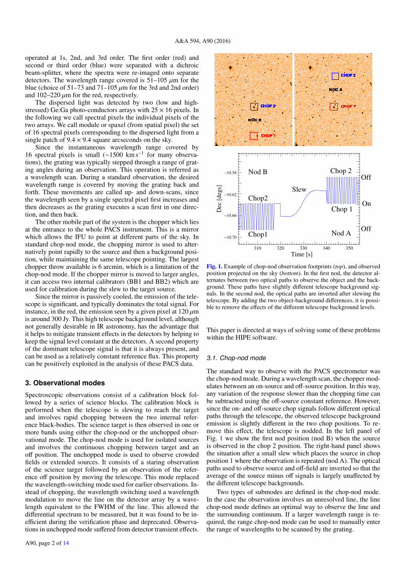
Fig. 1. Example of chop-nod observation footprints (top), and observedposition projected on the sky (bottom). In the first nod, the detector al-ternates between two optical paths to observe the object and the back-ground. These paths have slightly different telescope background sig-nals. In the second nod, the optical paths are inverted after slewing thetelescope. By adding the two object-background differences, it is possi-ble to remove the effects of the different telescope background levels.

This paper is directed at ways of solving some of these problemswithin the HIPE software.

3.1. Chop-nod mode

The standard way to observe with the PACS spectrometer wasthe chop-nod mode. During a wavelength scan, the chopper mod-ulates between an on-source and off-source position. In this way,any variation of the response slower than the chopping time canbe subtracted using the off-source constant reference. However,since the on- and off-source chop signals follow different opticalpaths through the telescope, the observed telescope backgroundemission is slightly different in the two chop positions. To re-move this effect, the telescope is nodded. In the left panel ofFig. 1 we show the first nod position (nod B) when the sourceis observed in the chop 2 position. The right-hand panel showsthe situation after a small slew which places the source in chopposition 1 where the observation is repeated (nod A). The opticalpaths used to observe source and off-field are inverted so that theaverage of the source minus off signals is largely unaffected bythe different telescope backgrounds.

Two types of submodes are defined in the chop-nod mode.In the case the observation involves an unresolved line, the linechop-nod mode defines an optimal way to observe the line andthe surrounding continuum. If a larger wavelength range is re-quired, the range chop-nod mode can be used to manually enterthe range of wavelengths to be scanned by the grating.

A90, page 2 of 14

D. Fadda et al.: Transient effects in Herschel/PACS spectroscopy

The data reduction is done on each individual pixel. The sim-plest reduction technique uses the calibration block to computethe average response during the observation. The response is de-fined for each pixel as the ratio between the measured and ex-pected signal from the internal calibrators which was measuredin the laboratory. The measured signal is composed of the tele-scope background (TA and TB in the two chopping positions),source flux (s), and dark (d) signal. The telescope background isdominated by the emission of the primary mirror, and dependson the temperature of the spot which is seen by the detector.Because of differential variations in the mirror temperature, andits emissivity with position on the mirror, the different chopperpositions tend to see differing degrees of telescope background.Although, during a given observation, the overall temperatureof the mirror changed slowly, it was measured to vary due tochanges in illumination of the spacecraft by the Sun on longertimescales than a single observation.

For the measured signal C, in V/s, in a chop-nod observationwe have:

C1 = (TA + d + s) · R(t) C2 = (TB + d) · R(t)

C′1 = (TA + d) · R(t) C′2 = (TB + d + s) · R(t) (1)

for the two chop positions in the first (C1 and C2) and secondnods (C′1 and C′2), respectively. Here R(t) = ρλ · r(t) is the prod-uct of the relative spectral response function (RSRF) ρλ and theresponse function r(t) (V s−1 Jy−1) which can vary with time.TA and TB correspond to the signal detected from the telescopebackground at the chopper positions A and B, respectively.

The simplest technique consists in estimating the signalsource by computing the differential signal, s, between the chop-ping positions and combining the nods:

s = [(C1 −C2) + (C′1 −C′2)]/(2 · ρλ · rCB), [Jy] (2)

where rCB = 〈r(t)〉 is the average response estimated from thecalibration block. As we can see, the method works if r(t) isapproximately constant during a chopping period (1 s) so that thesubtraction cancels the effect of a transient. This approach wasused by the so called SPG (standard product generation) pipelineto populate the Herschel Science Archive (HSA) for chop-nodobservations2 until recently.

Since SPG 13, an alternative approach exploiting the knowl-edge of the telescope background is used. This technique doesnot require the application of the RSRF and response correctionssince it uses the ratios between the observations in the two chop-ping directions. Nevertheless, the accuracy of the results dependson the knowledge of the mean telescope background. Also, ra-tios introduce more noise in the final signal with respect to thestandard reduction.

In formulae, if we define normalization as:

N =C1 −C2

C1 + C2+

C′1 −C′2C′1 + C′2

=2s

TA + TB + 2d + s, (3)

the signal normalized to the average telescope background canbe expressed as:

s〈T 〉 + d

=s

(TA + TB)/2 + d=

N1 − N/2

· (4)

The source flux can be therefore derived by multiplying thenormalized signal by the telescope background (dark included).

2 http://www.cosmos.esa.int/web/herschel/science-archive

This method frees the result from the effects of the variable re-sponse although it requires the knowledge of the dark. SincePACS has no shutter, the dark was measured in the laboratorybefore the launch of Herschel. It is not known with great accu-racy although its value is negligible with respect to the telescopebackground. The telescope background was derived in flight bycalibrating the emission of the mirror with observed spectra ofbright asteroids.

3.2. Unchopped mode

At the end of the verification phase, the wavelength switchingmode (see Poglitsch et al. 2010) was released3 and used in a fewkey programs. Several disadvantages became apparent with thismode during its early use, leading to its replacement with theunchopped mode. For example, by construction, the continuumof the source could not be measured. Moreover, only observa-tions of unresolved lines could be measured correctly. Asym-metric lines or lines broader than the wavelength switching in-terval were found to be difficult to recover. For large wavelengthranges, SED shape variations can lead to peculiar baselines inthe final differential spectrum. This made observations over largewavelength ranges challenging. Finally, the rapid switching ofthe grating between two distant wavelength positions createdmechanical oscillations which required a long time to damp.This effect was more severe in space than during ground test-ing, leading to longer time intervals between useful observa-tional samples and thus preventing an efficient removal of rapidresponse variations.

It appeared clear that performing a slow grating scan whilestaring at an object, followed by a similar observation pointedto an off position, yielded superior results compared withwavelength-switching. This unchopped mode had the advantageof allowing large wavelength range scans, such as far-IR SEDsof confused or extended regions. Unlike the chop-nod mode,where the two chopper positions sample different optical pathsand therefore different mirror temperatures, in the unchoppedmode the optical paths used for on- and off-source observationsare the same. Therefore, the mirror temperature in the on- andoff-source are exactly the same. Moreover, in the case of chop-nod, the footprint of the detector on the sky rotates slightly be-tween the two chop positions (see the PACS observer manual,Fig. 4.7). The effect, though small, is worse for the larger chop-per throws. This means that in the two nod positions, the onlyspaxel seeing precisely the same part of the source is the centralone. Spaxels further from the center become successively mis-matched in the two nods. So, the reduction works best for thecentral spaxel. This problem does not exist for the unchoppedmode because the observation of the on- and off-positions aremade with a fixed central chopper position.

The unchopped line and range modes were released onSeptember 2010, superseding the previous wavelength switchingmode4. A specific unchopped mode for bright lines was releasedon April 20115.

3 herschel.esac.esa.int/Docs/AOTsReleaseStatus/PACS_WaveSwitching_ReleaseNote_20Jan2010.pdf4 herschel.esac.esa.int/Docs/AOTsReleaseStatus/PACS_Unchopped_ReleaseNote_20Sep2010.pdf5 herschel.esac.esa.int/twiki/pub/Public/PacsAotReleaseNotes/PACS_UnchoppedReleaseNote_BrightLines_15Apr2011.pdf Note that all the AOT releasenotes will be provided on the Herschel Legacy Library website startingfrom 2017.

A90, page 3 of 14

A&A 594, A90 (2016)

20 30 40 50 60 70 80 90 100 110

0.85

0.90

0.95

1.00

1.05

1.10

20 30 40 50 60 70 80 90 100 110

0.85

0.90

0.95

1.00

1.05

1.10

10 20 30 40 50 60 70 80 90 100 110 1200.0

0.5

1.0

1.5

2.0

2.5

Time [s] Time [s]

0 10 20 30 40 50 60 70 80 90 100 110 120

Flu

x /

<F

lux

>

Blue array

BB2

BB1

Blue array

BB1

values

Previous

Calibration block

BB2

Obs

Previous

values

Calibration block

BB2

BB1

Transient

1

2

3

4

5

6

7

8

9

10

Observation

Flu

x [

V/s

]

Red array

BB2BB1

Red array

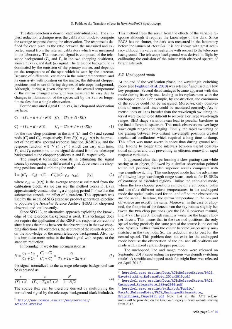
Fig. 2. Transients affecting the calibration block for the red (left) and blue (right) arrays. During the calibration block, the detectors see alternativelythe two blackbodies (top panels). Since the initial flux is significantly different from the fluxes of the internal blackbodies, a strong transient occursduring the first minute of the observation. The signals normalized to the median values of each blackbody (bottom panels) show how the sametransient affects the fluxes from the two blackbodies (blue and red lines). The transient effect is more pronounced for the red array.

In unchopped mode, a complete wavelength scan is done firston the on-source (hereafter ON) position and then later on a off-source (hereafter OFF) position clear of source emission. Unfor-tunately, variations of the response during the ON scan cannotbe corrected using the OFF scan because the two scans are per-formed at different times. So, although unchopped observationsoffer some advantages over the chop-nod mode, the effects oftransients require mitigation. In this paper, we show the typicaltransients found in the signal, and some techniques to model andsubtract them.

Three different sub-modes exist for the unchopped mode:

– unchopped line, for single line observations.– unchopped bright line, for single bright lines. It is 30% more

time efficient than the standard line mode since bright linesrequire less continuum to compute the line intensity.

– unchopped range, for observations of the continuum or acomplex of lines.

A further difference between these sub-modes is that the refer-ence OFF is observed during the same AOR (Astronomical Ob-servation Request) in the case of the unchopped line, but has tobe provided as a separate AOR in the unchopped range. In orderto ensure the observations are performed sequentially, the OFFobservation in the unchopped range scan is concatenated to themain observation within the observation sequence.

4. Transients

The term transient refers to a delayed response of a detectorto the variation of the incident flux. Transients are particularly

evident after sudden variations of flux on detector arrays (see,e.g., Coulais & Abergel 2000). In Fig. 2 we show the signaldetected during the calibration block when the chopper pointsalternatively between the two internal black bodies (which havedifferent temperatures). Passing from the previous observation tothe internal black bodies causes a clear transient effect which ismore important in the case of the red array (left panels). Whenthe signal is normalized to the asymptotic flux (bottom panels),the response variation becomes evident. It is interesting to note(left bottom panel) that the short transients due to cosmic hits onthe array have a timescale longer than the chopping time. Thisallows the correction of these effects using the chop-node mode.

We can classify three separate types of transients:

– continuum-jump transients: transients due to a suddenchange of the incident flux from one almost constant levelto another almost constant level;

– cosmic ray transients: transients induced by cosmic ray hitswhich produce glitches, followed by a response variation;

– scan dependent transients: transients along a wavelengthscan produced by rapid variations of the (dominant) tele-scope background and continuum (in the case of a brighttarget).

It is worth mentioning that the Standard Product Generation(SPG) pipeline, which populates the HSA, does not use any typeof transient correction. So the products available in the archivefor the frequency switched and unchopped-mode observationscontain many transient effects that could adversely affect sciencegoals. However, from HIPE 14 onward, users have the option of

A90, page 4 of 14

D. Fadda et al.: Transient effects in Herschel/PACS spectroscopy

processing their data with special scripts designed specifically tocorrect transients. The current paper describes how these correc-tions are made. In the following we describe in detail the differ-ent types of transients.

4.1. Continuum-jump transients

A sudden change in the illumination of a detector pixel passingfrom one flux level to another, can induce a major transient inthe signal. This occurs typically at the beginning of each obser-vation just after the completion of the calibration block. Becauseof the difference between the flux from internal calibrators andthe telescope background, a transient is usually visible duringthe entire observation.

Another common form of this kind of transients is when achange of band, or change of wavelength occurs while observinga source. For example, the user may have requested two differ-ent lines occurring at different wavelengths. When the grating iscommanded to access a different part of the spectrum, or changeto a completely different region of the spectrum, a jump in thesignal usually occurs because of the changing emission spec-trum of the telescope background at different wavelengths (seeSect. 5.2). If the source is very bright, differences in continuumlevel from the source can also induce a transient.

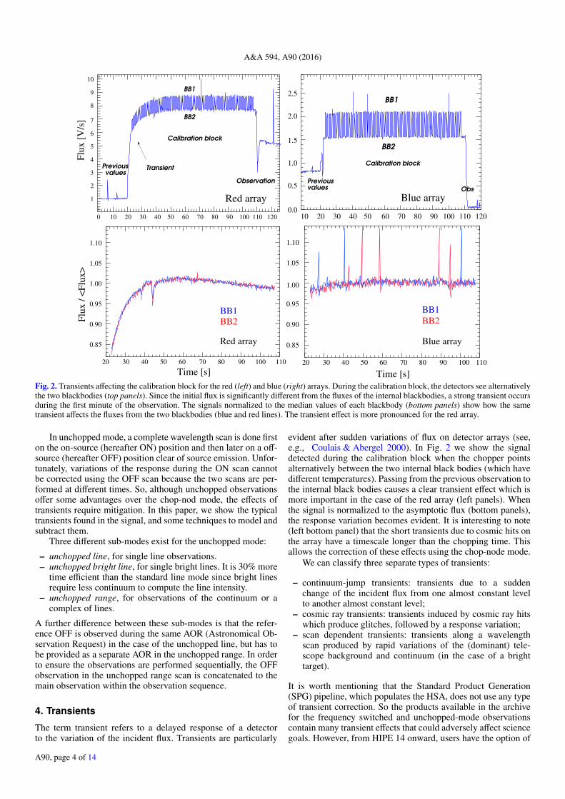
If the source continuum is negligible with respect to the tele-scope background, it is possible to normalize the signal duringthe whole observation to the telescope background which hasbeen previously calibrated. The transient due to the jump in con-tinuum between the calibration block and the target observationappears clearly, see Fig. 3. It is possible, in this case, to fit thebehaviour with a model and subtract it from the observation. It isinteresting to note that, without this correction, an OFF observa-tion can have a measured flux greater than an ON observation ifit happens to be performed during a period of response stabiliza-tion. This effect is not taken into account by the SPG pipeline,so that many observations in the archive have an artificial andconfusing negative background.

Some observations that used the unchopped mode containedrequests for more than one band in a single AOR. For extendedsources, a typical raster observation allows one to cover an ex-tended region by moving the telescope to cover a grid of posi-tions. However, for efficiency reasons, the AOR was designedto cycle through all the requested bands at each raster position,before moving the telescope to the next position in the rastersequence. An unexpected side effect of this strategy was thegeneration of transients at each band change. It is not possibleto remove these jump-transients in a clean way in case of suchmultiple-band observations.

There is an important lesson to be learned from this expe-rience with PACS. In retrospect, it would have been better toobserve the complete raster in a single band, before cycling tothe next band. This would have minimized the effects of band-induced jump-transient. We advise that any future mission wheretransient could be an issue, should avoid as much as possiblesudden changes in flux during the observation. This is probablythe case of FIFI-LS onboard SOFIA, which is essentially a cloneof the PACS spectrograph. Unfortunately, when the observa-tional mode was introduced for Herschel, the reduction pipelinewas not fully developed, and it was very difficult to evaluate allthe effects. Since the response was known to stabilize relativelyfast, it was assumed that the effect of a band change was mini-mal, compared with the advantage of being more time efficient.Experience later showed that jump-transient transient caused byband changes appear to limit the quality of the observation, even

0.00 0.05 0.10 0.15

0.9

51.0

01.0

51.1

01.1

50.0 0.3 0.6 0.9 1.2 1.5 1.8

0.9

51.0

01.0

51.1

01.1

51.2

0Time [hour]

Sig

nal / T

elB

kg

Fig. 3. When the signals from a spaxel are normalized to the ex-pected telescope background a long-term transient after the calibra-tion block becomes clear. In this example (an observation of M81,ObsID 1342269535) an OFF position is observed at the beginning andat the end of the observation (blue dots), while a 2×2 raster observationis performed in the middle (green dots). Since the continuum emissionof the object is negligible with respect to the telescope background, itis possible to fit the general long-term transient (red line) and correctthe signal. Note that many huge transients appear in individual spectralpixels because of cosmic ray hits on the detectors. If this correction isnot made, and an average background is subtracted from the signal, thefinal image will present an artificial gradient and the flux will be nega-tive in some regions. Top inset panel: a close-up of the initial part of thesignal just after the calibration block, showing the strong transient. Theperiodic variation in the signal is a left-over from the imperfect tele-scope background estimate used for normalization. The empty spacesbetween points occur during telescope slewing.

with the most advanced data reduction. Indeed, we are able to seejump-transients even in the blue channel, which has the fastestresponse stabilization compared with the red (see Fig. 4).

4.2. Cosmic ray transients

It is well known that for Ge:Ga detectors, energetic cosmic raysusually produce glitches in the signal, followed by response vari-ations. Depending on the energy of the cosmic ray, the glitchcan be followed by a tail or the variation can be more compli-cated (lowering temporarily the response). A similar behaviorwas noted in the past for pixels in the ISOCAM array on the In-frared Space Observatory (see, for example, Lari et al. 2001).We will show that the response variation can be described witha combination of exponential functions (see Sect. 5). The mainchallenge to correcting and masking the damage in the signalfrom cosmic ray hits is to select the most significant events, andthen find the starting time which marks the beginning of the dis-continuity in the signal.

A90, page 5 of 14

A&A 594, A90 (2016)

Drift

CR transients

Time [hours]

Sig

nal

/ T

elB

kg

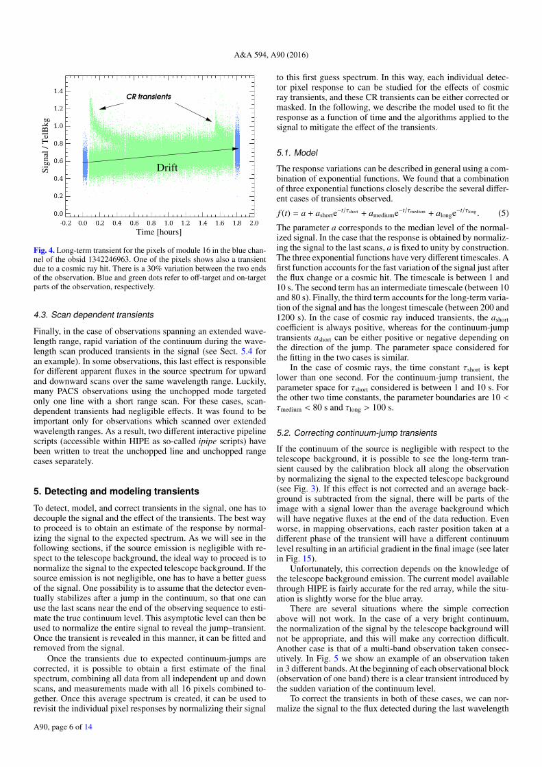
Fig. 4. Long-term transient for the pixels of module 16 in the blue chan-nel of the obsid 1342246963. One of the pixels shows also a transientdue to a cosmic ray hit. There is a 30% variation between the two endsof the observation. Blue and green dots refer to off-target and on-targetparts of the observation, respectively.

4.3. Scan dependent transients

Finally, in the case of observations spanning an extended wave-length range, rapid variation of the continuum during the wave-length scan produced transients in the signal (see Sect. 5.4 foran example). In some observations, this last effect is responsiblefor different apparent fluxes in the source spectrum for upwardand downward scans over the same wavelength range. Luckily,many PACS observations using the unchopped mode targetedonly one line with a short range scan. For these cases, scan-dependent transients had negligible effects. It was found to beimportant only for observations which scanned over extendedwavelength ranges. As a result, two different interactive pipelinescripts (accessible within HIPE as so-called ipipe scripts) havebeen written to treat the unchopped line and unchopped rangecases separately.

5. Detecting and modeling transients

To detect, model, and correct transients in the signal, one has todecouple the signal and the effect of the transients. The best wayto proceed is to obtain an estimate of the response by normal-izing the signal to the expected spectrum. As we will see in thefollowing sections, if the source emission is negligible with re-spect to the telescope background, the ideal way to proceed is tonormalize the signal to the expected telescope background. If thesource emission is not negligible, one has to have a better guessof the signal. One possibility is to assume that the detector even-tually stabilizes after a jump in the continuum, so that one canuse the last scans near the end of the observing sequence to esti-mate the true continuum level. This asymptotic level can then beused to normalize the entire signal to reveal the jump–transient.Once the transient is revealed in this manner, it can be fitted andremoved from the signal.

Once the transients due to expected continuum-jumps arecorrected, it is possible to obtain a first estimate of the finalspectrum, combining all data from all independent up and downscans, and measurements made with all 16 pixels combined to-gether. Once this average spectrum is created, it can be used torevisit the individual pixel responses by normalizing their signal

to this first guess spectrum. In this way, each individual detec-tor pixel response to can be studied for the effects of cosmicray transients, and these CR transients can be either corrected ormasked. In the following, we describe the model used to fit theresponse as a function of time and the algorithms applied to thesignal to mitigate the effect of the transients.

5.1. Model

The response variations can be described in general using a com-bination of exponential functions. We found that a combinationof three exponential functions closely describe the several differ-ent cases of transients observed.

f (t) = a + ashorte−t/τshort + amediume−t/τmedium + alonge−t/τlong . (5)

The parameter a corresponds to the median level of the normal-ized signal. In the case that the response is obtained by normaliz-ing the signal to the last scans, a is fixed to unity by construction.The three exponential functions have very different timescales. Afirst function accounts for the fast variation of the signal just afterthe flux change or a cosmic hit. The timescale is between 1 and10 s. The second term has an intermediate timescale (between 10and 80 s). Finally, the third term accounts for the long-term varia-tion of the signal and has the longest timescale (between 200 and1200 s). In the case of cosmic ray induced transients, the ashortcoefficient is always positive, whereas for the continuum-jumptransients ashort can be either positive or negative depending onthe direction of the jump. The parameter space considered forthe fitting in the two cases is similar.

In the case of cosmic rays, the time constant τshort is keptlower than one second. For the continuum-jump transient, theparameter space for τshort considered is between 1 and 10 s. Forthe other two time constants, the parameter boundaries are 10 <τmedium < 80 s and τlong > 100 s.

5.2. Correcting continuum-jump transients

If the continuum of the source is negligible with respect to thetelescope background, it is possible to see the long-term tran-sient caused by the calibration block all along the observationby normalizing the signal to the expected telescope background(see Fig. 3). If this effect is not corrected and an average back-ground is subtracted from the signal, there will be parts of theimage with a signal lower than the average background whichwill have negative fluxes at the end of the data reduction. Evenworse, in mapping observations, each raster position taken at adifferent phase of the transient will have a different continuumlevel resulting in an artificial gradient in the final image (see laterin Fig. 15).

Unfortunately, this correction depends on the knowledge ofthe telescope background emission. The current model availablethrough HIPE is fairly accurate for the red array, while the situ-ation is slightly worse for the blue array.

There are several situations where the simple correctionabove will not work. In the case of a very bright continuum,the normalization of the signal by the telescope background willnot be appropriate, and this will make any correction difficult.Another case is that of a multi-band observation taken consec-utively. In Fig. 5 we show an example of an observation takenin 3 different bands. At the beginning of each observational block(observation of one band) there is a clear transient introduced bythe sudden variation of the continuum level.

To correct the transients in both of these cases, we can nor-malize the signal to the flux detected during the last wavelength

A90, page 6 of 14

D. Fadda et al.: Transient effects in Herschel/PACS spectroscopy

−0.05 0.00 0.05 0.10 0.15 0.20 0.25 0.300

50

100

150

200

250

300

On−source Off−source

Band 3

Band 1Band 2

Band 3

Band 1

Band 2

Transients

Time [hours]

No

rmal

ized

sig

nal

[Jy

]

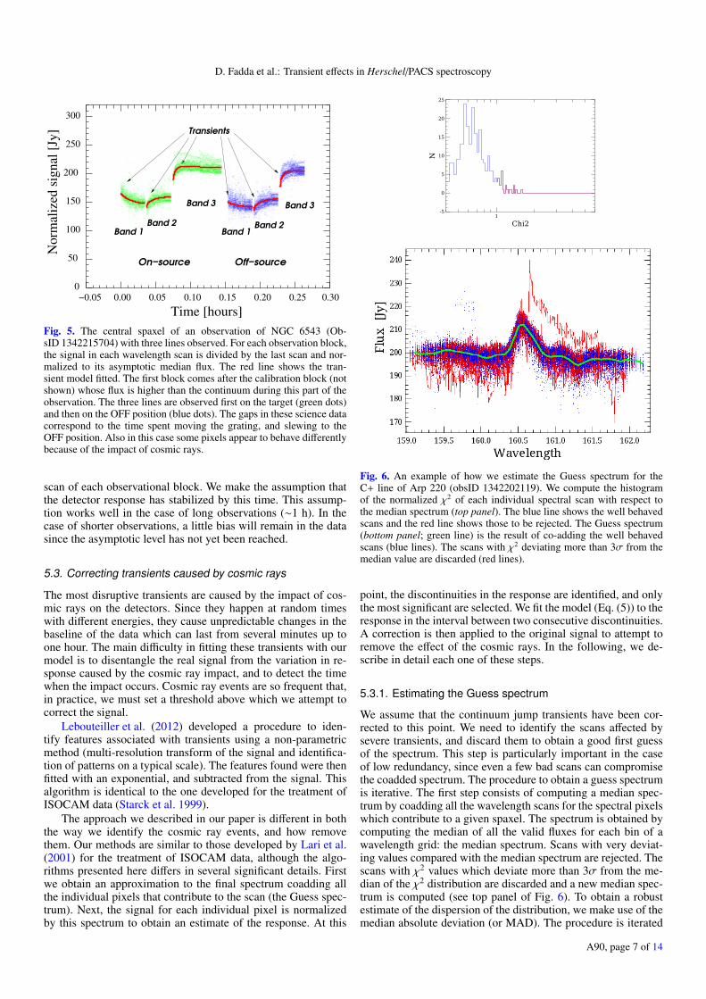
Fig. 5. The central spaxel of an observation of NGC 6543 (Ob-sID 1342215704) with three lines observed. For each observation block,the signal in each wavelength scan is divided by the last scan and nor-malized to its asymptotic median flux. The red line shows the tran-sient model fitted. The first block comes after the calibration block (notshown) whose flux is higher than the continuum during this part of theobservation. The three lines are observed first on the target (green dots)and then on the OFF position (blue dots). The gaps in these science datacorrespond to the time spent moving the grating, and slewing to theOFF position. Also in this case some pixels appear to behave differentlybecause of the impact of cosmic rays.

scan of each observational block. We make the assumption thatthe detector response has stabilized by this time. This assump-tion works well in the case of long observations (∼1 h). In thecase of shorter observations, a little bias will remain in the datasince the asymptotic level has not yet been reached.

5.3. Correcting transients caused by cosmic rays

The most disruptive transients are caused by the impact of cos-mic rays on the detectors. Since they happen at random timeswith different energies, they cause unpredictable changes in thebaseline of the data which can last from several minutes up toone hour. The main difficulty in fitting these transients with ourmodel is to disentangle the real signal from the variation in re-sponse caused by the cosmic ray impact, and to detect the timewhen the impact occurs. Cosmic ray events are so frequent that,in practice, we must set a threshold above which we attempt tocorrect the signal.

Lebouteiller et al. (2012) developed a procedure to iden-tify features associated with transients using a non-parametricmethod (multi-resolution transform of the signal and identifica-tion of patterns on a typical scale). The features found were thenfitted with an exponential, and subtracted from the signal. Thisalgorithm is identical to the one developed for the treatment ofISOCAM data (Starck et al. 1999).

The approach we described in our paper is different in boththe way we identify the cosmic ray events, and how removethem. Our methods are similar to those developed by Lari et al.(2001) for the treatment of ISOCAM data, although the algo-rithms presented here differs in several significant details. Firstwe obtain an approximation to the final spectrum coadding allthe individual pixels that contribute to the scan (the Guess spec-trum). Next, the signal for each individual pixel is normalizedby this spectrum to obtain an estimate of the response. At this

Fig. 6. An example of how we estimate the Guess spectrum for theC+ line of Arp 220 (obsID 1342202119). We compute the histogramof the normalized χ2 of each individual spectral scan with respect tothe median spectrum (top panel). The blue line shows the well behavedscans and the red line shows those to be rejected. The Guess spectrum(bottom panel; green line) is the result of co-adding the well behavedscans (blue lines). The scans with χ2 deviating more than 3σ from themedian value are discarded (red lines).

point, the discontinuities in the response are identified, and onlythe most significant are selected. We fit the model (Eq. (5)) to theresponse in the interval between two consecutive discontinuities.A correction is then applied to the original signal to attempt toremove the effect of the cosmic rays. In the following, we de-scribe in detail each one of these steps.

5.3.1. Estimating the Guess spectrum

We assume that the continuum jump transients have been cor-rected to this point. We need to identify the scans affected bysevere transients, and discard them to obtain a good first guessof the spectrum. This step is particularly important in the caseof low redundancy, since even a few bad scans can compromisethe coadded spectrum. The procedure to obtain a guess spectrumis iterative. The first step consists of computing a median spec-trum by coadding all the wavelength scans for the spectral pixelswhich contribute to a given spaxel. The spectrum is obtained bycomputing the median of all the valid fluxes for each bin of awavelength grid: the median spectrum. Scans with very deviat-ing values compared with the median spectrum are rejected. Thescans with χ2 values which deviate more than 3σ from the me-dian of the χ2 distribution are discarded and a new median spec-trum is computed (see top panel of Fig. 6). To obtain a robustestimate of the dispersion of the distribution, we make use of themedian absolute deviation (or MAD). The procedure is iterated

A90, page 7 of 14

A&A 594, A90 (2016)

4200 4400 4600 4800 5000 5200

0.85

0.90

0.95

1.00

1.05

1.10

1.15

1.20

Frame No.

Res

ponse

190

195

200

205

210

215

220

225

230

235

240

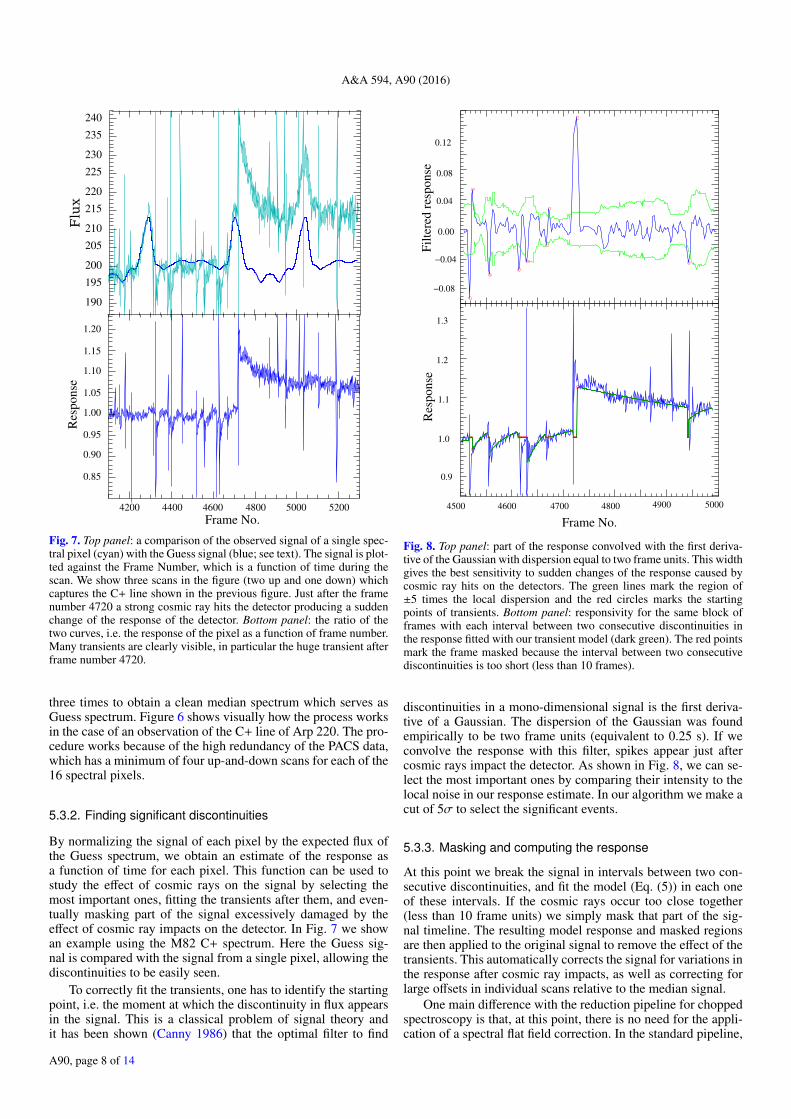
Fig. 7. Top panel: a comparison of the observed signal of a single spec-tral pixel (cyan) with the Guess signal (blue; see text). The signal is plot-ted against the Frame Number, which is a function of time during thescan. We show three scans in the figure (two up and one down) whichcaptures the C+ line shown in the previous figure. Just after the framenumber 4720 a strong cosmic ray hits the detector producing a suddenchange of the response of the detector. Bottom panel: the ratio of thetwo curves, i.e. the response of the pixel as a function of frame number.Many transients are clearly visible, in particular the huge transient afterframe number 4720.

three times to obtain a clean median spectrum which serves asGuess spectrum. Figure 6 shows visually how the process worksin the case of an observation of the C+ line of Arp 220. The pro-cedure works because of the high redundancy of the PACS data,which has a minimum of four up-and-down scans for each of the16 spectral pixels.

5.3.2. Finding significant discontinuities

By normalizing the signal of each pixel by the expected flux ofthe Guess spectrum, we obtain an estimate of the response asa function of time for each pixel. This function can be used tostudy the effect of cosmic rays on the signal by selecting themost important ones, fitting the transients after them, and even-tually masking part of the signal excessively damaged by theeffect of cosmic ray impacts on the detector. In Fig. 7 we showan example using the M82 C+ spectrum. Here the Guess sig-nal is compared with the signal from a single pixel, allowing thediscontinuities to be easily seen.

To correctly fit the transients, one has to identify the startingpoint, i.e. the moment at which the discontinuity in flux appearsin the signal. This is a classical problem of signal theory andit has been shown (Canny 1986) that the optimal filter to find

4500 4600 4700 4800 4900 5000

0.9

1.0

1.1

1.2

1.3

0.00

−0.04

−0.08

0.04

0.08

0.12

Frame No.

Res

ponse

Fil

tere

d r

esponse

Fig. 8. Top panel: part of the response convolved with the first deriva-tive of the Gaussian with dispersion equal to two frame units. This widthgives the best sensitivity to sudden changes of the response caused bycosmic ray hits on the detectors. The green lines mark the region of±5 times the local dispersion and the red circles marks the startingpoints of transients. Bottom panel: responsivity for the same block offrames with each interval between two consecutive discontinuities inthe response fitted with our transient model (dark green). The red pointsmark the frame masked because the interval between two consecutivediscontinuities is too short (less than 10 frames).

discontinuities in a mono-dimensional signal is the first deriva-tive of a Gaussian. The dispersion of the Gaussian was foundempirically to be two frame units (equivalent to 0.25 s). If weconvolve the response with this filter, spikes appear just aftercosmic rays impact the detector. As shown in Fig. 8, we can se-lect the most important ones by comparing their intensity to thelocal noise in our response estimate. In our algorithm we make acut of 5σ to select the significant events.

5.3.3. Masking and computing the response

At this point we break the signal in intervals between two con-secutive discontinuities, and fit the model (Eq. (5)) in each oneof these intervals. If the cosmic rays occur too close together(less than 10 frame units) we simply mask that part of the sig-nal timeline. The resulting model response and masked regionsare then applied to the original signal to remove the effect of thetransients. This automatically corrects the signal for variations inthe response after cosmic ray impacts, as well as correcting forlarge offsets in individual scans relative to the median signal.

One main difference with the reduction pipeline for choppedspectroscopy is that, at this point, there is no need for the appli-cation of a spectral flat field correction. In the standard pipeline,

A90, page 8 of 14

D. Fadda et al.: Transient effects in Herschel/PACS spectroscopyF

lux

120

110

140

150

160

170

180

190

200

130

1800 2600 2800240022002000

120

110

100

140

150

160

170

180

190

130

Flu

x

Frame No.

SPG

TC

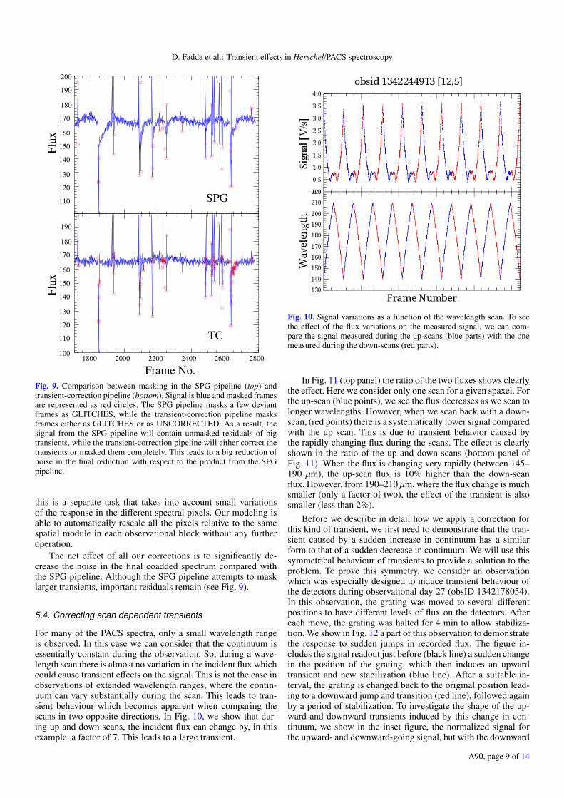
Fig. 9. Comparison between masking in the SPG pipeline (top) andtransient-correction pipeline (bottom). Signal is blue and masked framesare represented as red circles. The SPG pipeline masks a few deviantframes as GLITCHES, while the transient-correction pipeline masksframes either as GLITCHES or as UNCORRECTED. As a result, thesignal from the SPG pipeline will contain unmasked residuals of bigtransients, while the transient-correction pipeline will either correct thetransients or masked them completely. This leads to a big reduction ofnoise in the final reduction with respect to the product from the SPGpipeline.

this is a separate task that takes into account small variationsof the response in the different spectral pixels. Our modeling isable to automatically rescale all the pixels relative to the samespatial module in each observational block without any furtheroperation.

The net effect of all our corrections is to significantly de-crease the noise in the final coadded spectrum compared withthe SPG pipeline. Although the SPG pipeline attempts to masklarger transients, important residuals remain (see Fig. 9).

5.4. Correcting scan dependent transients

For many of the PACS spectra, only a small wavelength rangeis observed. In this case we can consider that the continuum isessentially constant during the observation. So, during a wave-length scan there is almost no variation in the incident flux whichcould cause transient effects on the signal. This is not the case inobservations of extended wavelength ranges, where the contin-uum can vary substantially during the scan. This leads to tran-sient behaviour which becomes apparent when comparing thescans in two opposite directions. In Fig. 10, we show that dur-ing up and down scans, the incident flux can change by, in thisexample, a factor of 7. This leads to a large transient.

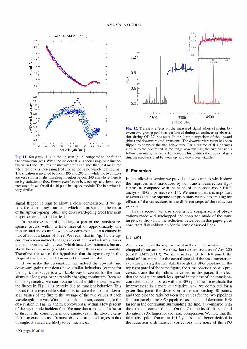
Fig. 10. Signal variations as a function of the wavelength scan. To seethe effect of the flux variations on the measured signal, we can com-pare the signal measured during the up-scans (blue parts) with the onemeasured during the down-scans (red parts).

In Fig. 11 (top panel) the ratio of the two fluxes shows clearlythe effect. Here we consider only one scan for a given spaxel. Forthe up-scan (blue points), we see the flux decreases as we scan tolonger wavelengths. However, when we scan back with a down-scan, (red points) there is a systematically lower signal comparedwith the up scan. This is due to transient behavior caused bythe rapidly changing flux during the scans. The effect is clearlyshown in the ratio of the up and down scans (bottom panel ofFig. 11). When the flux is changing very rapidly (between 145–190 µm), the up-scan flux is 10% higher than the down-scanflux. However, from 190–210 µm, where the flux change is muchsmaller (only a factor of two), the effect of the transient is alsosmaller (less than 2%).

Before we describe in detail how we apply a correction forthis kind of transient, we first need to demonstrate that the tran-sient caused by a sudden increase in continuum has a similarform to that of a sudden decrease in continuum. We will use thissymmetrical behaviour of transients to provide a solution to theproblem. To prove this symmetry, we consider an observationwhich was especially designed to induce transient behaviour ofthe detectors during observational day 27 (obsID 1342178054).In this observation, the grating was moved to several differentpositions to have different levels of flux on the detectors. Aftereach move, the grating was halted for 4 min to allow stabiliza-tion. We show in Fig. 12 a part of this observation to demonstratethe response to sudden jumps in recorded flux. The figure in-cludes the signal readout just before (black line) a sudden changein the position of the grating, which then induces an upwardtransient and new stabilization (blue line). After a suitable in-terval, the grating is changed back to the original position lead-ing to a downward jump and transition (red line), followed againby a period of stabilization. To investigate the shape of the up-ward and downward transients induced by this change in con-tinuum, we show in the inset figure, the normalized signal forthe upward- and downward-going signal, but with the downward

A90, page 9 of 14

A&A 594, A90 (2016)

Fig. 11. Top panel: flux in the up-scan (blue) compared to the flux inthe down-scan (red). When the incident flux is decreasing (blue line be-tween 140 and 195 µm) the measured flux is higher than that measuredwhen the flux is increasing (red line in the same wavelength region).The situation is inverted between 195 and 205 µm, while the two fluxesare very similar in the wavelength region beyond 205 µm where there isno big variation in flux. Bottom panel: ratio between up- and down-scanmeasured fluxes for all the 16 pixel in a space module. The behaviour isvery similar.

signal flipped in sign to allow a close comparison. If we ig-nore the cosmic ray transients which are present, the behaviorof the upward-going (blue) and downward-going (red) transientresponses are almost identical.

In the above example, the largest part of the transient re-sponse occurs within a time interval of approximately oneminute, and the example we chose corresponded to a change influx of about a factor of three. We recall that in Fig. 11, the up-and-down scan induced changes in continuum which were largerthan this over the whole scan (which lasted two minutes), but areabout the same order (roughly a factor of three) in one minute.Therefore, the test of the hypothesis that the symmetry in theshape of the upward and downward transient is valid.

If we make the assumption that indeed the upward- anddownward-going transients have similar behaviors (except forthe sign), this suggests a workable way to correct for the tran-sients in a long scan over a rapidly changing continuum. Becauseof the symmetry, we can assume that the differences betweenthe fluxes in Fig. 11 is entirely due to transient behavior. Thismeans that a reasonable solution is to scale the up- and down-scan values of the flux to the average of the two values at eachwavelength interval. With this simple solution, according to theobservation in Fig. 12, the flux recovered is within a few percentof the asymptotic incident flux. We note that a change of a factorof three in the continuum in one minute (as in the above exam-ple) is an extreme case. In most observations, the changes in fluxthroughout a scan are likely to be much less.

0.8

0.9

1.0

1.1

No

rmali

zed

Flu

x

400 8000

Frame No.

450035002500

Frame No.

0.3

0.6

0.9

1.2

Flu

xFig. 12. Transient effects on the measured signal when changing be-tween two grating positions performed during an engineering observa-tion during OD 27 (see text). In the inset, comparison of the upward(blue) and downward (red) transients. The downward transient has beenflipped to compare the two behaviours. For a regime of flux changessimilar to the one found in the range observations, the two transientsfollow essentially the same behaviour. This justifies the choice of get-ting the median signal between up- and down-scan signals.

6. Examples

In the following section we provide a few examples which showthe improvements introduced by our transient-correction algo-rithms, as compared with the standard unchopped-mode HIPEanalysis (SPG pipeline, vers. 14). We remind that it is importantto avoid executing pipeline scripts blindly without examining theeffects of the corrections in the different steps of the reductionprocess.

In this section we also show a few comparisons of obser-vations made with unchopped and chop-nod mode of the sametargets, to show how the reduction described in this paper givesconsistent flux calibration for the same observed lines.

6.1. Line

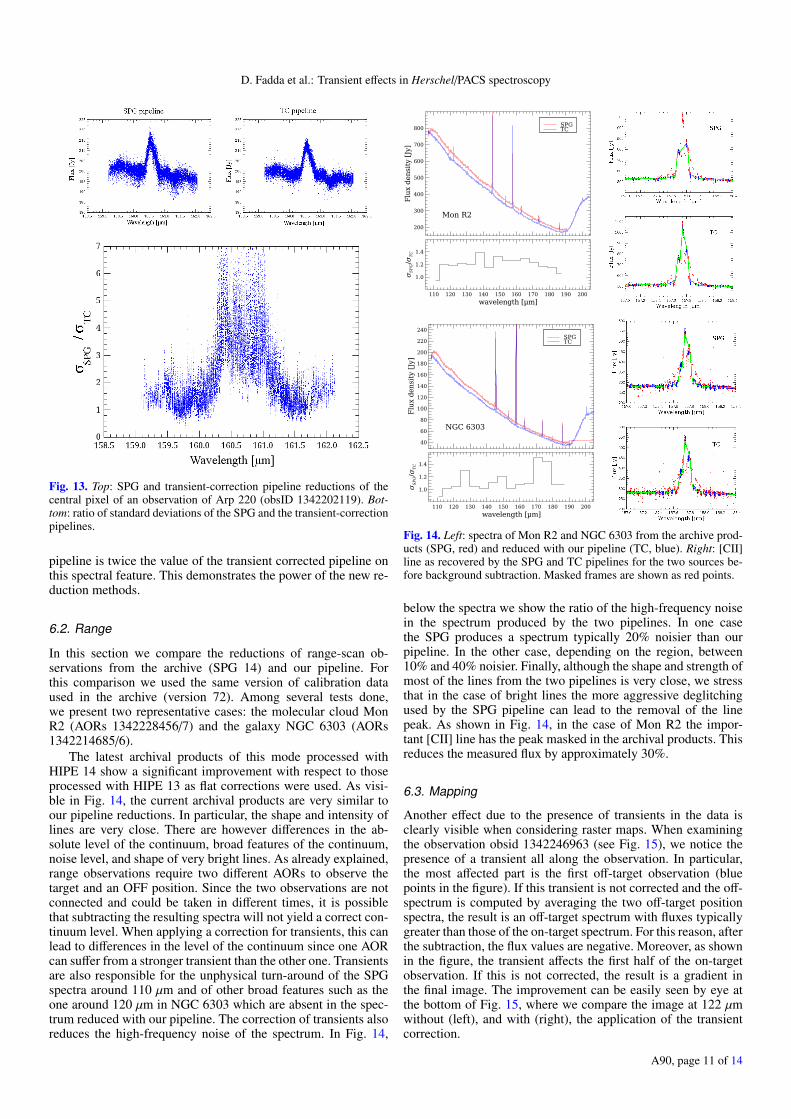
As an example of the improvement in the reduction of a line un-chopped observation, we show here an observation of Arp 220(obsID 1342202119). We show in Fig. 13 (top left panel) thecloud of flux-points for the central spaxel of the spectrometer ar-ray after passing the raw data through the SPG pipeline. In thetop right panel of the same figure, the same observation was pro-cessed using the algorithms described in this paper. It is clearthat the points are much less spread in the case of the transient–corrected data compared with the SPG pipeline. To evaluate theimprovement in a more quantitative way, we computed for agiven flux point, the dispersion in the surrounding 30 points,and then plot the ratio between the values for the two pipelines(bottom panel). The SPG pipeline has a standard deviation 40%larger in the continuum surrounding the line, as compared withthe transient-corrected data. On the C+ line itself, the standarddeviation is 3× larger for the same comparison. We note that thefaint absorption feature at 161.3 µm is much better defined inthe reduction with transient corrections. The noise of the SPG

A90, page 10 of 14

D. Fadda et al.: Transient effects in Herschel/PACS spectroscopy

Fig. 13. Top: SPG and transient-correction pipeline reductions of thecentral pixel of an observation of Arp 220 (obsID 1342202119). Bot-tom: ratio of standard deviations of the SPG and the transient-correctionpipelines.

pipeline is twice the value of the transient corrected pipeline onthis spectral feature. This demonstrates the power of the new re-duction methods.

6.2. Range

In this section we compare the reductions of range-scan ob-servations from the archive (SPG 14) and our pipeline. Forthis comparison we used the same version of calibration dataused in the archive (version 72). Among several tests done,we present two representative cases: the molecular cloud MonR2 (AORs 1342228456/7) and the galaxy NGC 6303 (AORs1342214685/6).

The latest archival products of this mode processed withHIPE 14 show a significant improvement with respect to thoseprocessed with HIPE 13 as flat corrections were used. As visi-ble in Fig. 14, the current archival products are very similar toour pipeline reductions. In particular, the shape and intensity oflines are very close. There are however differences in the ab-solute level of the continuum, broad features of the continuum,noise level, and shape of very bright lines. As already explained,range observations require two different AORs to observe thetarget and an OFF position. Since the two observations are notconnected and could be taken in different times, it is possiblethat subtracting the resulting spectra will not yield a correct con-tinuum level. When applying a correction for transients, this canlead to differences in the level of the continuum since one AORcan suffer from a stronger transient than the other one. Transientsare also responsible for the unphysical turn-around of the SPGspectra around 110 µm and of other broad features such as theone around 120 µm in NGC 6303 which are absent in the spec-trum reduced with our pipeline. The correction of transients alsoreduces the high-frequency noise of the spectrum. In Fig. 14,

Fig. 14. Left: spectra of Mon R2 and NGC 6303 from the archive prod-ucts (SPG, red) and reduced with our pipeline (TC, blue). Right: [CII]line as recovered by the SPG and TC pipelines for the two sources be-fore background subtraction. Masked frames are shown as red points.

below the spectra we show the ratio of the high-frequency noisein the spectrum produced by the two pipelines. In one casethe SPG produces a spectrum typically 20% noisier than ourpipeline. In the other case, depending on the region, between10% and 40% noisier. Finally, although the shape and strength ofmost of the lines from the two pipelines is very close, we stressthat in the case of bright lines the more aggressive deglitchingused by the SPG pipeline can lead to the removal of the linepeak. As shown in Fig. 14, in the case of Mon R2 the impor-tant [CII] line has the peak masked in the archival products. Thisreduces the measured flux by approximately 30%.

6.3. Mapping

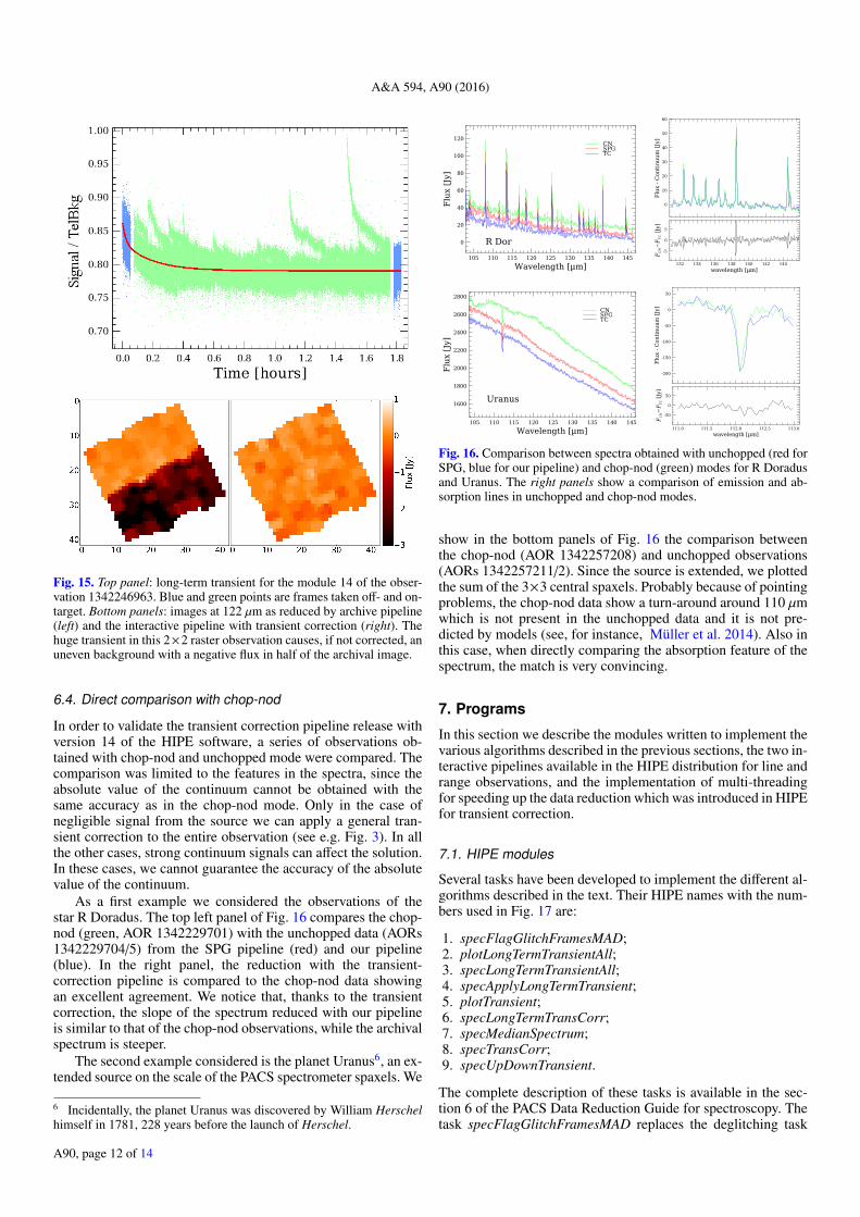
Another effect due to the presence of transients in the data isclearly visible when considering raster maps. When examiningthe observation obsid 1342246963 (see Fig. 15), we notice thepresence of a transient all along the observation. In particular,the most affected part is the first off-target observation (bluepoints in the figure). If this transient is not corrected and the off-spectrum is computed by averaging the two off-target positionspectra, the result is an off-target spectrum with fluxes typicallygreater than those of the on-target spectrum. For this reason, afterthe subtraction, the flux values are negative. Moreover, as shownin the figure, the transient affects the first half of the on-targetobservation. If this is not corrected, the result is a gradient inthe final image. The improvement can be easily seen by eye atthe bottom of Fig. 15, where we compare the image at 122 µmwithout (left), and with (right), the application of the transientcorrection.

A90, page 11 of 14

A&A 594, A90 (2016)

Fig. 15. Top panel: long-term transient for the module 14 of the obser-vation 1342246963. Blue and green points are frames taken off- and on-target. Bottom panels: images at 122 µm as reduced by archive pipeline(left) and the interactive pipeline with transient correction (right). Thehuge transient in this 2×2 raster observation causes, if not corrected, anuneven background with a negative flux in half of the archival image.

6.4. Direct comparison with chop-nod

In order to validate the transient correction pipeline release withversion 14 of the HIPE software, a series of observations ob-tained with chop-nod and unchopped mode were compared. Thecomparison was limited to the features in the spectra, since theabsolute value of the continuum cannot be obtained with thesame accuracy as in the chop-nod mode. Only in the case ofnegligible signal from the source we can apply a general tran-sient correction to the entire observation (see e.g. Fig. 3). In allthe other cases, strong continuum signals can affect the solution.In these cases, we cannot guarantee the accuracy of the absolutevalue of the continuum.

As a first example we considered the observations of thestar R Doradus. The top left panel of Fig. 16 compares the chop-nod (green, AOR 1342229701) with the unchopped data (AORs1342229704/5) from the SPG pipeline (red) and our pipeline(blue). In the right panel, the reduction with the transient-correction pipeline is compared to the chop-nod data showingan excellent agreement. We notice that, thanks to the transientcorrection, the slope of the spectrum reduced with our pipelineis similar to that of the chop-nod observations, while the archivalspectrum is steeper.

The second example considered is the planet Uranus6, an ex-tended source on the scale of the PACS spectrometer spaxels. We

6 Incidentally, the planet Uranus was discovered by William Herschelhimself in 1781, 228 years before the launch of Herschel.

Fig. 16. Comparison between spectra obtained with unchopped (red forSPG, blue for our pipeline) and chop-nod (green) modes for R Doradusand Uranus. The right panels show a comparison of emission and ab-sorption lines in unchopped and chop-nod modes.

show in the bottom panels of Fig. 16 the comparison betweenthe chop-nod (AOR 1342257208) and unchopped observations(AORs 1342257211/2). Since the source is extended, we plottedthe sum of the 3×3 central spaxels. Probably because of pointingproblems, the chop-nod data show a turn-around around 110 µmwhich is not present in the unchopped data and it is not pre-dicted by models (see, for instance, Müller et al. 2014). Also inthis case, when directly comparing the absorption feature of thespectrum, the match is very convincing.

7. Programs

In this section we describe the modules written to implement thevarious algorithms described in the previous sections, the two in-teractive pipelines available in the HIPE distribution for line andrange observations, and the implementation of multi-threadingfor speeding up the data reduction which was introduced in HIPEfor transient correction.

7.1. HIPE modules

Several tasks have been developed to implement the different al-gorithms described in the text. Their HIPE names with the num-bers used in Fig. 17 are:

1. specFlagGlitchFramesMAD;2. plotLongTermTransientAll;3. specLongTermTransientAll;4. specApplyLongTermTransient;5. plotTransient;6. specLongTermTransCorr;7. specMedianSpectrum;8. specTransCorr;9. specUpDownTransient.

The complete description of these tasks is available in the sec-tion 6 of the PACS Data Reduction Guide for spectroscopy. Thetask specFlagGlitchFramesMAD replaces the deglitching task

A90, page 12 of 14

D. Fadda et al.: Transient effects in Herschel/PACS spectroscopy

Level 0

Level 0.5

Level 1

Level 2

Common spectrometer processing modules

MAD deglitcher (1)

Dark, RSRF, Response

Plot long-term transient (2,3)

Can we fit wholeobservation transient ?

Correct whole observation transient (4)

Correct continuum-jump transients (6)

Correct cosmic-ray transients (7,8)

Mask outliers

Subtract off position

Common spectrometer projection block

NOYES

Line unchopped pipelineLevel 0

Level 0.5

Level 1

Common spectrometer processing modules

MAD deglitch (1)

Dark, RSRF, Response

Correct scan transient (9)

Correct continuum-jump transients (6)

Correct cosmic-ray transients (7,8)

Mask outliers

Range unchopped pipeline

Fig. 17. Flow-charts of the unchopped pipelines for the line and range modes (left and right, respectively). In the range mode the pipeline stops atlevel 1 products. In fact, two observations are required to complete the data reduction since the on-target and off-target observations are executedin different AORs. The numbers in brackets correspond to the tasks used for the step as described in Sect. 7.1.

specFlagGlitchFramesQTest used in the chop-nod pipeline. Thechop-nod task masks glitches and part of the resulting transient.In our case, we want to preserve these data to fit our transientmodel. We achieve this result by computing the local noise andmasking only outliers beyond a given threshold. The task spec-LongTermTransientAll fits the transient along the whole historyof the pixel (see Fig. 3). The fits of transients during scienceblocks are performed by the task specLongTermTransCorr (seeFig. 5). The task specMedianSpectrum evaluates the Guess spec-trum (see Fig. 6). An important bug in this task has been cor-rected in HIPE 15 (build 2845). Transients caused by cosmic rayhits are treated with the task specTransCor (see Figs. 7 and 8).This task creates a new mask (UNCORRECTED) which con-tains the part of the signal which cannot be fitted by our modelsince the interval between two consecutive discontinuities con-tains less than 10 points. Finally, the correction of scan depen-dent transients described in Sect. 5.4 is implemented in the taskspecUpDownTransient.

The unchopped transient correction pipelines make use ofMINPACK, a robust package for minimization. MINPACK ismore robust in its handling of inaccurate initial estimates ofthe parameter values than other conventional methods. Weimplemented MINPACK in HIPE as the MinpackPro LeastSquares Fitting Library. This implementation is based on theoriginal public domain version by Moré et al. (1980)7. OurJAVA version is based on a translation to the C languageby S. Moshier8. MinpackPro contains enhancements borrowed

7 http://www.netlib.org/minpack8 https://heasarc.gsfc.nasa.gov/ftools/caldb/help/HDmpfit.html

from C. Markwardt’s IDL fitting routine MPFIT9 (see alsoMarkwardt 2009).

7.2. HIPE pipelines

The flow-chart of the pipelines for the reduction of line and rangeunchopped data is shown in Fig. 17. In the case of the line mode,one AOR contains the on- and off-target observations. So, thepipeline goes from the raw data to the final projected spectra.We suggest to set the parameter interactive to True in order totrigger the interactive step described in the flow-chart to check ifthe transient across the entire observation is correctable. This pa-rameter is set to False in the script to allow for automatic checksof the pipeline during software updates.

In the case of the range mode, the main difference is the pres-ence of the transient correction due to the rapid change of thetelescope background during a wavelength scan. Also, the cor-rection of the whole observation transient is not necessary sincerange-mode AOR contain only a on- or off-target observation.For this reason, the range-mode pipeline stops at level 1 prod-ucts. To obtain level 2 products, one has to combine the reduc-tion of the on- and off-target AORs using the combine on-offscript available under the pipeline unchopped range scan menu.

7.3. Multi-threading

Since transient correction tasks are computationally intensive,we created the multi-threading framework ThreadByRange in

9 http://purl.com/net/mpfit

A90, page 13 of 14

A&A 594, A90 (2016)

HIPE to exploit the increasing availability of multiple cores inmodern computers. This multi-threading framework takes ad-vantage of the organization of the PACS data. In the pipeline,data are stored as Frames, i.e. time ordered sets of signal, wave-length, etc. for the 25 × 16 pixels. Frames are then organizedin blocks called Slices which correspond to the different partsof an observation (e.g. the calibration block, off-target observa-tions, several raster positions, etc.). The correction tasks can runon each spaxel independently, so that it is possible to run 25 par-allel processes. On the top of that, each Slice can be processedindependently. Therefore, we organize the threads into two poolsof threads for processing. One pool is for threads dedicated toprocessing the Slices, the other to operate on each spaxel. Re-source usage can be controlled by specifying the pool sizes astask parameters. The default is to create two threads for process-ing Slices and a number of threads for the spaxels equal to halfof the CPUs available.

The tasks implemented in HIPE require a combination of se-rial and parallel processes. Taking the signal from or applyingthe correction to Frames must be done serially, since the resultsof asynchronous updates to shared objects are undefined. Threemethods are defined in ThreadByRange to interact with data:

– preApply() Initialization that must be done serially for thecomputational unit. In the case of pipeline tasks, this involvescopying signal, wavelengths, masks, etc. to memory that isaccessed exclusively by the apply() method.

– apply() ThreadByRange schedules this method to be appliedin parallel. All of the work applied to spaxels in parallel isdone here, such as minimizations, discontinuity detection,application of corrections, etc.

– postApply() ThreadByRange calls this method after the com-pletion of each work unit. Transient correction tasks use thismethod to update Frames with the correction for each spaxel.

An absolute requirement for multi-threading is thread safety ofthe classes defined in the transient correction tasks. Fortunately,the level of thread safety was easy to determine due to the robust,clean design of the numerical package of HIPE.

Our multi-thread framework ThreadByRange sits on the JavaConcurrency Package from which we use the JAVA Execu-torCompletionService for synchronization, and the Executors’fixedThreadPool for scheduling. In the processing of spaxels orSlices, a Callable is created for each computational unit and issubmitted to the CompletionService. This service synchronizeson task completion by using the BlockingQueue to retrieve com-pleted tasks as Futures. For a complete description of the Javaclasses Callable, Executor, BlockingQueue, Futures, and of thismechanism see Goetz (2006, Sect. 6.3.5 “Java Completion Ser-vice: Executor meets BlockingQueue”).

8. Summary and conclusion

We presented a description of transient effects on the responseof the PACS spectroscopy detectors. Taking into account these

effects is paramount in the case of observations using the un-chopped modes. In fact, contrary to the chop-nod mode, there isno way to cancel these effects by constantly monitoring an off-target signal since on-target and off-target observations are madeat different times.

We showed how it is possible to disentangle and treat sep-arately transients due to different effects and how to improvedramatically the signal-to-noise ratio of the final products withrespect to those from the Herschel archive. In particular, in theline mode the signal-to-noise ratio of lines can easily triple. Inthe case of range-mode, the correction of transients can lead tochanges of slope, smoother spectra, and better reconstructionsof bright lines. The algorithms described in the paper have beenimplemented in programs available in HIPE since version 14,as part of the drop-down menu for so-called interactive (ipipe)scripts. In particular, two different pipelines scripts are availablefor the reduction of line and range unchopped modes. An impor-tant bug affecting the range unchopped mode was corrected inHIPE version 15 (build 2845).

Acknowledgements. The Herschel spacecraft was designed, built, tested, andlaunched under a contract to ESA managed by the Herschel/Planck Project teamby an industrial consortium under the overall responsibility of the prime con-tractor Thales Alenia Space (Cannes), and including Astrium (Friedrichshafen)responsible for the payload module and for system testing at spacecraft level,Thales Alenia Space (Turin) responsible for the service module, and Astrium(Toulouse) responsible for the telescope, with in excess of a hundred subcontrac-tors. HCSS and HIPE are a joint developments by the Herschel Science GroundSegment Consortium, consisting of ESA, the NASA Herschel Science Center,and the HIFI, PACS and SPIRE consortia. We are grateful to the entire spec-troscopy group of PACS for their help and support. In particular, we would liketo acknowledge P. Royer and B. Vanderbusche for testing the pipeline and point-ing out significant bugs, as well as A. Poglitsch, R. Vavrek, A. Contursi, and J.de Jong for many useful discussions. We thank K. Exter and the anonymous ref-eree for their careful reading of the manuscript and very useful suggestions. Wewould like to thank B. Ali and R. Paladini for their constant support at the NASAHerschel Science Center. Finally, D.F. is indebted to Prof. I. Perez-Fournon forhis support at the IAC in a particularly difficult moment of his scientific carrier.

ReferencesCanny, J. 1986, IEEE Transactions on Pattern Analysis and Machine

Intelligence, 8, 679Coulais, A., & Abergel, A. 2000, A&AS, 141, 533Fadda, D., Marleau, F. R., Storrie-Lombardi, L. J., et al. 2006, AJ, 131, 2859Goetz, B. 2006, Java Concurrency in Practice (New York: Addison-Wesley

Professional)Lari, C., Pozzi, F., Gruppioni, C., et al. 2001, MNRAS, 325, 1173Lebouteiller, V., Cormier, D., Madden, S. C., et al. 2012, A&A, 548, A91Markwardt, C. B. 2009, in Astronomical Data Analysis Software and Systems

XVIII, eds. D. A. Bohlender, D. Durand, & P. Dowler, ASP Conf. Ser., 411,251

Moré, J., Garbow, B., & Hillstrom, K. 1980, Technical Report Argonne NationalLaboratory, 80, 74

Müller, T., Balog, Z., Nielbock, M., et al. 2014, Exp. Astron., 37, 253Ott, S. 2010, in Astronomical Data Analysis Software and Systems XIX, eds.

Y. Mizumoto, K.-I. Morita, & M. Ohishi, ASP Conf. Ser., 434, 139Pilbratt, G. L., Riedinger, J. R., Passvogel, T., et al. 2010, A&A, 518, L1Poglitsch, A., Waelkens, C., Geis, N., et al. 2010, A&A, 518, L2Starck, J. L., Aussel, H., Elbaz, D., Fadda, D., & Cesarsky, C. 1999, A&AS, 138,

365

A90, page 14 of 14