A survey of the theory of coherent lowerprevisions

Enrique Miranda∗

Abstract

This paper presents a summary of Peter Walley’s theory of coherent lower pre-visions. We introduce three representations of coherent assessments: coherentlower and upper previsions, closed and convex sets of linear previsions, and setsof desirable gambles. We show also how the notion of coherence can be used toupdate our beliefs with new information, and a number of possibilities to modelthe notion of independence with coherent lower previsions. Next, we comment onthe connection with other approaches in the literature: de Finetti’s and Williams’earlier work, Kuznetsov’s and Weischelberger’s work on interval-valued probabil-ities, Dempster-Shafer theory of evidence and Shafer and Vovk’s game-theoreticapproach. Finally, we present a brief survey of some applications and summarizethe main strengths and challenges of the theory.

Keywords. Subjective probability, imprecision, avoiding sure loss, coherence, desir-ability, conditional lower previsions, independence.

1 IntroductionThis paper aims at presenting the main facts about the theory of coherent lower previ-sions. This theory falls within the subjective approach to probability, where the prob-ability of an event represents our information about how likely is this event to happen.This interpretation of probability is mostly used in the framework of decision making,and is sometimes referred to as epistemic probability [30, 43].

Subjective probabilities can be given a number of different interpretations. One ofthem is the behavioural one we consider in this paper: the probability of an event isinterpreted in terms of some behaviour that depends on the appearance of the event,for instance as betting rates on or against the event, or buying and selling prices on theevent.

The main goal of the theory of coherent lower previsions is to provide a number ofrationality criteria for reasoning with subjective probabilities. By reasoning we shallmean here the cognitive process aimed at solving problems, reaching conclusions ormaking decisions. The rationality of some reasoning can be characterised by means of

∗Rey Juan Carlos University, Dept. of Statistics and Operations Research. C-Tulipan, s/n. 28933Mostoles (Spain). e-mail: enrique.miranda@urjc.es

1

a number of principles and standards that determine the quality of the reasoning. In thecase of probabilistic reasoning, one can consider two different types of rationality. Theinternal one, which studies to which extent our model is self-consistent, is modelledin Walley’s theory using the notion of coherence. But there is also an external part ofrationality, which studies whether our model is consistent with the available evidence.The allowance for imprecision in Walley’s theory is related to this type of rationality.

Within the subjective approach to probability, there are two problems that mayaffect the estimation of the probability of an event: those of indeterminacy and incom-pleteness. Indeterminacy, also called indeterminate uncertainty in [34], happens whenthere exist events which are not equivalent for our subject, but for which he has nopreference, meaning that he cannot decide if he would bet on one over the other. Itcan be due for instance to lack of information, conflicting beliefs, or conflicting infor-mation. On the other hand, incompleteness is due to difficulties in the elicitation ofthe model, meaning that our subject may not be capable of estimating the subjectiveprobability of an event with an arbitrary degree of precision. This can be caused by alack of introspection or a lack of assessment strategies, or to the limits of the computa-tional abilities. Both indeterminacy and incompleteness are a source of imprecision inprobability models.

One of the first to talk about the presence of imprecision when modelling uncer-tainty was Keynes in [33], although there were already some comments about it in ear-lier works by Bernoulli and Lambert [58]. Keynes considered an ordering between theprobability of the different outcomes of an experiment which need only be partial. Hisideas were later formalized by Koopman in [35, 36, 37]. Other work in this directionwas made by Borel [4], Smith [61], Good [31], Kyburg [43] and Levi [45]. In 1975,Williams [85] made a first attempt to make a detailed study of imprecise subjectiveprobability theory, based on the work that de Finetti had done on subjective probability[21, 23] and considering lower and upper previsions instead of precise previsions. Thiswas developed in much more detail by Walley in [71], who established the arguablymore mature theory that we shall survey here.

The terms indeterminate or imprecise probabilities are used in the literature to referto any model using upper or lower probabilities on some domain, i.e., for a model wherethe assumption of the existence of a precise and additive probability model is dropped.In this sense, we can consider credal sets [45], 2- and n-monotone set functions [5],possibility measures [15, 27, 88], p-boxes [29], fuzzy measures [26, 32], etc. Ourfocus here is on what we shall call the behavioural theory of coherent lower previsions,as developed by Peter Walley in [71]. We are interested in this model mainly for tworeasons: from a mathematical point of view, it subsumes most of the other models in theliterature as particular cases, having therefore a unifying character. On the other hand,it also has a clear interpretation in terms of acceptable transactions. This interpretationlends itself naturally to decision making [71, Section 3.9]. Our aim in this paper is togive a gentle introduction to the theory for the reader who first approaches the field, andto serve him as a guide on his way through. However, this work by no means pretendsto be an alternative to Walley’s book, and we refer to [71] for a much more detailedaccount of the properties we shall present and for a thorough justification of the theory.

In order to ease the transition for the interested reader from this survey to Walley’sbook, let us give a short outline of the different chapters of the book. The book starts

2

with an introduction to reasoning and behavior in Chapter 1. Chapter 2 introduces co-herent lower and upper previsions, and studies their main properties. Chapter 3 showshow to coherently extend our assessments, through the notion of natural extension, andprovides also the expression in terms of sets of linear previsions or almost-desirablegambles. Chapter 4 discusses the assessment and the elicitation of imprecise probabili-ties. Chapter 5 studies the different sources of imprecision in probabilities, investigatesthe adequacy of precise models for cases of complete ignorance and comments onother imprecise probability models. The study of conditional lower and upper previ-sions starts in Chapter 6, with the definition of separate coherence and the coherenceof an unconditional and a conditional lower prevision. This is generalized in Chapter 7to the case of a finite number of conditional lower previsions, focusing on a number ofstatistical models. Chapter 8 establishes a general theory of natural extension of severalcoherent conditional previsions. Finally, Chapter 9 is devoted to the modelling of thenotion of independence.

In this paper, we shall summarize the main aspects of this book and the relation-ships between Walley’s theory of coherent lower previsions and some other approachesto imprecise probabilities. The paper is structured as follows: in Section 2, we presentthe main features of unconditional coherent lower previsions. We give three represen-tations of the available information: coherent lower and upper previsions, sets of desir-able gambles, and sets of linear previsions, and show how to extend the assessments tolarger domains. In Section 3, we outline how we can use the theory of coherent lowerprevisions to update the assessments with new information, and how to combine infor-mation from different sources. Thus, we make a study of conditional lower previsions.Section 4 is devoted to the notion of independence. In Section 5, we compare Walley’stheory with other approaches to subjective probability: the seminal work of de Finetti,first generalized to the imprecise case by Williams, Kuznetsov’s and Weischelberger’swork on interval-valued probabilities, the Dempster-Shafer theory of evidence, andShafer and Vovk’s recent work on game-theoretic probability. In Section 6, we reviewa number of applications. We conclude the paper in Section 7 with an overview ofsome questions and remaining challenges in the field.

2 Coherent lower previsions and other equivalent rep-resentations

In this section, we present the main facts about coherent lower previsions, their be-havioural interpretation and the notion of natural extension. We show that the infor-mation provided by a coherent lower prevision can also be expressed by means of aset of linear previsions or by a set of desirable gambles. Although this last approachis arguably better suited to understanding the ideas behind the behavioural interpreta-tion, we have opted for starting with the notion of coherent lower previsions, becausethis will help to understand the differences with classical probability theory and more-over they will be the ones we use when talking about conditional lower previsions inSection 3. We refer to [20] for an alternative introduction.

3

2.1 Coherent lower previsionsConsider a non-empty space Ω, representing the set of outcomes of an experiment. Thebehavioural theory of imprecise probabilities provides tools to model our informationabout the likelihood of the different outcomes in terms of our betting behavior on somegambles that depend on these outcomes. Specifically, a gamble f on Ω is a boundedreal-valued function on Ω. It represents an uncertain reward, meaning that we obtainthe price f (ω) if the outcome of the experiment is ω ∈ Ω. This reward is expressedin units of some linear utility scale, see [71, Section 2.2] for details. We shall denoteby L (Ω) the set of gambles on Ω.1 A particular case of gambles are the indicators ofevents, that is, the gambles IA defined by IA(ω) = 1 if ω ∈ A and IA(ω) = 0 otherwisefor some A⊆Ω.

Example 1. Jack has made it to the final of a TV contest. He has already won 50000euros,2 and he can add to this the amount he gets by playing with The Magic Urn.He must draw a ball from the urn, and he wins or loses money depending on itscolor: if he draws a green ball, he gets 10000 euros; if he draws a red ball, he gets5000 euros; and if he draws a black ball, he gets nothing. Mathematically, the setof outcomes of the experiment Jack is going to make (drawing a ball from the urn)is Ω = green,red,black, and the gamble f1 which determines his prize is given byf1(green) = 10000, f1(red) = 5000, f1(black) = 0.

Let K be a set of gambles on Ω. A lower prevision on K is a functional P :K → R. For any gamble f in K , P( f ) represents a subject’s supremum acceptablebuying price for f ; this means that he is disposed to pay P( f )− ε for the uncertainreward determined by f and the outcome of the experiment, or, in other words, that thetransaction f −P( f )+ ε , understood as a point-wise operation, is acceptable to himfor every ε > 0 (however, nothing is said about whether he would buy f for the priceP( f )).3

Given a gamble f we can also consider our subject’s infimum acceptable sellingprice for f , which we shall denote by P( f ). It means that the transaction P( f )+ ε− fis acceptable to him for every ε > 0 (but nothing is said about the transaction P( f )− f ).We obtain in this way an upper prevision P( f ) on some set of gambles K ′.

We shall see in Section 2.3 an equivalent formulation of lower and upper previsionsin terms of sets of desirable gambles. For the time being, and in order to justify therationality requirements we shall introduce, we shall only assume the following:

1. A transaction that makes our subject lose utiles, no matter the outcome of theexperiment, is not acceptable for him.

1Although Walley’s theory assumes the variables involved are bounded, the theory has also been general-ized to unbounded random variables in [63, 62]. The related formulation of the theory from a game-theoreticpoint of view, as we will present it in Section 5.6, has also been made for arbitrary gambles. See alsoSection 5.3.

2Such an amount of money is only added in order to justify the linearity of the utility scale, which in thecase of money only holds if the amounts at stake are small compared to the subject’s capital.

3In this paper, we use Walley’s notation of P for lower previsions and P for upper previsions; these canbe seen as lower and upper expectations, and will only be interpreted as lower and upper probabilities whenthe gamble f is the indicator of some event.

4

2. If he considers acceptable a transaction, he should also accept any other transac-tion that gives him a greater reward, no matter the outcome of the experiment.

3. A positive linear combination of acceptable transactions should also be accept-able.

Example 1(cont.). If Jack pays x euros in order to play at The Magic Urn, then theincrease in his wealth is given by 10000− x euros if he draws a green ball, 5000− xeuros if he draws a red ball, and of −x euros if he draws a black ball (i.e., he loses xeuros in that case). The supremum amount of money that he is disposed to pay willbe his lower prevision for the gamble f1. If for instance he is certain that there are noblack balls in the urn, he should be disposed to pay as much as 5000 euros, becausehis wealth is not going to decrease, no matter which color is the ball he draws. Andif he has no additional information about the composition of the urn and wants to becautious, he will not pay more than 5000 euros, because it could happen that all theballs in the urn are red, and by paying more than 5000 euros he would end up alwayslosing money.

On the other hand, and after Jack has drawn a ball from the urn, and before he seesthe color, he can sell the unknown prize attached to it to the 2nd ranked player (Kate)for y euros. If Jack does this, his increase in wealth will be y−10000 euros if the ballis green, y−5000 euros if the ball is red, and y euros if the ball is black. The minimumamount of money that he requires in order to sell it will be his upper prevision for thegamble f1. If he knows that there are only red and green balls in the urn, he shouldaccept to sell it for more than 10000 euros, because he is not going to lose money bythis, but not for less: it could be that all the balls are green and then by selling it forless that 10000 euros he would end up losing money, no matter the outcome.

Since by selling a gamble f for a price µ or alternatively by buying the gamble − ffor the price −µ our subject increases his wealth in µ− f in both cases, it may be ar-gued that he should be disposed to accept these transactions under the same conditions.Hence, his infimum acceptable selling price for f should agree with the opposite of hissupremum acceptable buying price for − f . As a consequence, given a lower previsionon a set of gambles K we can define an upper prevision P on −K := − f : f ∈K ,by P(− f ) = −P( f ), and vice versa. Taking this into account, all the developmentsfor lower previsions can also be done for upper previsions, and vice versa. We shallconcentrate in this survey on lower previsions.

Lower previsions are subject to a number of rationality criteria, which assure theconsistency of the judgements they represent. First of all, a positive linear combinationof a number of acceptable gambles should never result in a transaction that makesour subject lose utiles, no matter the outcome. This is modeled through the notion ofavoiding sure loss: for every natural number n≥ 0 and f1, . . . , fn in K , we should have

supω∈Ω

n

∑i=1

[ fi(ω)−P( fi)]≥ 0.

Otherwise, there would exist some δ > 0 such that ∑ni=1[ fi(ω)− (P( fi)− δ )] ≤ −δ ,

meaning that the sum of acceptable transactions [ fi− (P( fi)−δ )] results in a loss of atleast δ , no matter the outcome of the experiment.

5

Example 1(cont.). Jack decides to pay 5000 euros in order to play at The Magic Urn.The TV host offers him also another prize depending on the same outcome: he will win9000 euros if he draws a black ball, 5000 if he draws a red ball and nothing if he drawsa green ball. Let f2 denote this other prize. Jack decides to pay additionally as muchas 5500 euros to also get this other prize. But then he is paying 10500 euros, and totalprize he is going to win is 10000 euros with a green or a red ball, and 9000 euros with ablack ball. Hence, he is going to lose money, no matter the outcome of the experiment.Mathematically, this means that the assessments P( f1) = 5000 and P( f2) = 5500 incura sure loss.

But there is a stronger requirement, namely that of coherence. Coherence meansthat our subject’s supremum acceptable buying price for a gamble f should not beraised by considering a positive linear combination of a finite number of other accept-able gambles. Formally, this means that for every non-negative integers n and m andgambles f0, f1, . . . , fn in K , we have

supω∈Ω

n

∑i=1

[ fi(ω)−P( fi)]−m[ f0(ω)−P( f0)]≥ 0. (1)

A lower prevision satisfying this condition will in particular avoid sure loss, by consid-ering the particular case of m = 0.

Let us suppose that Equation (1) does not hold for some non-negative integers n,mand some f0, . . . , fn in K . If m = 0, this means that P incurs in a sure loss, which wehave already argued is an inconsistency. Assume then that m > 0. Then there existssome δ > 0 such that

n

∑i=1

[ fi(ω)− (P( fi)−δ )]≤ m[ f0(ω)− (P(ω)+δ )]

for all ω ∈Ω. The left-hand side is a positive linear combination of acceptable buyingtransactions, which should then be acceptable. The right-hand side, which gives abigger reward than this acceptable transaction, should be acceptable as well. But thismeans that our subject should be disposed to buy the gamble f0 at the price P( f0)+δ ,which is greater than the supremum buying price he established before. This is aninconsistency.

Example 1(cont.). After thinking again, Jack decides to pay as much as 5000 euros forthe first prize ( f1) and 4000 euros for the second ( f2). He also decides that he willsell this second prize to Kate for anything bigger than 6000 euros, but not for less.In the language of lower and upper previsions, this means that P( f1) = 5000,P( f2) =4000,P( f2) = 6000, or, equivalently, P(− f2) =−6000. The rise in his wealth is givenby the following table:

6

green red blackBuy f1 for 5000 5000 0 −5000Buy f2 for 4000 −4000 1000 5000Sell f2 for 6000 6000 1000 −3000

Table 1: Increase on Jack’s wealth depending on the color of the ball he draws.

These assessments avoid sure loss. However, the first one already implies that heshould sell f2 for anything bigger than 5000 euros: if he does so, the increase in hiswealth is 5000 euros with a green ball, 0 with a red ball, and −4000 with a black ball.This situation is better than the one produced by buying f1 for 5000 euros, which heconsidered acceptable. This is an inconsistency with his assessment of 6000 euros asinfimum acceptable selling price for f2.

When the domain K of a lower prevision is a linear space, i.e., closed underaddition of gambles and multiplication of gambles by real numbers, coherence takesa simpler form. It can be checked that in that case P is coherent if and only if thefollowing three axioms hold for all f ,g in K and all λ > 0:

(P1) P( f )≥ inf f [accepting sure gains].

(P2) P(λ f ) = λP( f ) [positive homogeneity].

(P3) P( f +g)≥ P( f )+P(g) [superlinearity].

A consequence of these axioms is that a convex combination, a lower envelope anda point-wise limit of coherent lower previsions is again a coherent lower prevision.

A coherent lower prevision defined on indicators of events only is called a coher-ent lower probability. The lower probability of an event A can also be seen as oursubject’s supremum betting rate on the event, where betting on A means that he gets1 if A appears and 0 if it does not; similarly, the upper probability of an event A canbe interpreted as our subject infimum betting rate against the event A. Here, in con-tradistinction with the usual approaches to classical probability theory, we start fromprevisions (of gambles) and deduce the probabilities (of events), instead of going fromprobabilities to previsions using some expectation operator (but see also [83] for a sim-ilar approach in the case of precise probabilities).

As Walley himself argues in [71, Section 2.11], the notion of coherence can beconsidered too weak to fully characterize the rationality of probabilistic reasoning. In-deed, other additional requirements could be added in order to achieve this: we mayfor instance use symmetry or independent principles, or the principle of direct infer-ence discussed in [71, Section 1.7.2]. In this sense, most of the notions of upper andlower probabilities considered in the literature (2- and n-monotone capacities, belieffunctions, necessity measures) are particular cases of coherent lower previsions. Nev-ertheless, the main point here is that coherence is a necessary condition for rationality,and that we should at least require our subject’s assessments to satisfy it. Other possi-ble rationality axioms, such as the notion of conglomerability, will be discussed laterin this paper.

7

The assessments expressed by means of a lower prevision can also be made in termsof two alternative representations: sets of linear previsions and sets of almost-desirablegambles.

2.2 Linear previsionsWhen the supremum buying price and the infimum selling price for a gamble f coin-cide, then the common value P( f ) := P( f ) = P( f ) is called a fair price or previsionfor f . More generally, a real-valued function defined on a set of gambles K is calleda linear prevision when for all natural numbers m,n and gambles f1, . . . , fm,g1, . . . ,gnin the domain,

supω∈Ω

[m

∑i=1

[ fi(ω)−P( fi)]−n

∑j=1

[g j(ω)−P(g j)]]≥ 0. (2)

Assume that this condition does not hold for certain gambles f1, . . . , fm,g1, . . . ,gnin K . Then there exists some δ > 0 such that

m

∑i=1

[ fi(ω)−P( fi)+δ ]+n

∑j=1

[P(g j)−g j +δ ]<−δ (3)

for all ω ∈ Ω. Since P( fi) is our subject’s supremum acceptable buying price for thegamble fi, he is disposed to pay P( fi)−δ for it, so the transaction fi−P( fi)+δ is ac-ceptable for him; on the other hand, since P(g j) is his infimum acceptable selling pricefor g j, he is disposed to sell it for the price P(g j)+δ , so the transaction P(g j)+δ −g jis acceptable. But Equation (3) tells us that the sum of these acceptable transactionsproduces a loss of at least δ , no matter the outcome of the experiment!

A linear prevision P is coherent, both when interpreted as a lower and as an upperprevision; the former means that P := P is a coherent lower prevision on K , the latterthat the functional P1 on −K := − f : f ∈K given by P1( f ) = −P(− f ) is a co-herent lower prevision on −K . However, not every functional which is coherent bothas a lower and as an upper prevision is a linear prevision. This is because coherenceas a lower prevision only guarantees that Equation (2) holds for n ≤ 1, and coherenceas an upper prevision only guarantees that the same equation holds for the case wherem ≤ 1. An example showing that these two properties do not imply that Equation (2)holds for all non-negative natural numbers n,m is the following:

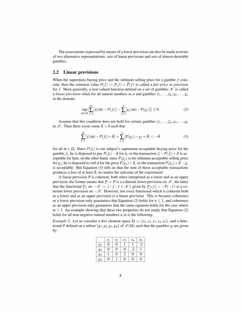
Example 2. Let us consider a five element space Ω := x1,x2,x3,x4,x5, and a func-tional P defined on a subset g1,g2,g3,g4 of L (Ω) such that the gambles gi are givenby:

x1 x2 x3 x4 x5g1 0 0 1 1 -2g2 0 0 0 -2 1g3 1 0 2 0 0g4 0 1 0 0 0

8

Consider P given by P(gi) = 0 for i = 1, . . . ,4. Then it can be checked that P iscoherent both as a lower and as an upper prevision. However, the gamble g1 + g2−g3− g4 has the constant value −1, and this implies that Equation (2) does not hold.Therefore P is not a linear prevision.

As it was the case with the coherence condition for lower previsions, when thedomain K satisfies some additional conditions, then Equation (2) can be simplified.For instance, if the domain K is self-conjugate, meaning that −K = K , then P is alinear prevision if and only if it avoids sure loss and satisfies P( f ) = −P(− f ) for allf ∈K . On the other hand, when K is a linear space of gambles, then P is a linearprevision if and only if

(P0) P( f +g) = P( f )+P(g) for all f ,g ∈K .

(P1) P( f )≥ inf f for all f ∈K .

It follows from these two conditions that P also satisfies

(P2) P(λ f ) = λP( f ) for all f ∈K ,λ > 0.

Hence, when the domain is a linear space of gambles linear previsions are coherentlower previsions which are additive instead of simply super-additive.

A linear prevision on a domain K is always the restriction of a linear prevision onall gambles, which is, by conditions (P0) and (P1), a linear functional on L (Ω). Weshall denote by P(Ω) the set of linear previsions on Ω.

Given a linear prevision P on all gambles, i.e., an element of P(Ω), we can con-sider its restriction Q to the set of indicators of events. This restriction can be seen inparticular as a functional on the class P(Ω) of subsets of Ω, using the identificationQ(A) = P(IA). It can be checked that this functional is a finitely additive probability,and P is simply the expectation with respect to Q. Hence, in case of linear previ-sions there is no difference in expressive power between representing the informationin terms of events or in terms of gambles: the restriction to events (the probability)determines the value on gambles (the expectation) and vice versa. This is no longertrue in the imprecise case, where there usually are infinitely many coherent extensionsof a coherent lower probability [71, Section 2.7.3], and this is why the theory is for-mulated in general in terms of gambles. The fact that lower previsions of events do notdetermine uniquely the lower previsions of gambles is due to the fact that we are notdealing with additive functionals anymore.

A linear prevision P whose domain is made up of the indicators of the events insome class A is called an additive probability on A . If in particular A is a fieldof events, then P is a finitely additive probability in the usual sense, and moreovercondition (2) simplifies to the usual axioms of finite additivity:

(a) P(A)≥ 0 for all A in A .

(b) P(Ω) = 1.

(c) P(A∪B) = P(A)+P(B) whenever A∩B = /0.

9

Example 1(cont.). Assume that Jack knows that there are only 10 balls in the urn,and that the drawing is fair, so that the probability of each color depends only on theproportion of balls of that color. If he knew the exact composition of the urn, forinstance that there are 5 green balls, 4 red balls and 1 black ball, then his expected gainwith the gamble f1 would be 0.5∗10000+0.4∗5000−0.1∗0 = 7000 euros, and thisshould be his fair price for the gamble. Any linear prevision will be determined by itsrestriction to events via the expectation operator. This restriction to events correspondsto some particular composition of the urn: if he knows that there are 4 red balls out of10 in the urn, then his betting rate on or against drawing a red ball (that is, his fair pricefor a gamble with reward 1 if he draws a red ball and 0 if he does not) should be 0.4.

We can characterize the coherence of a lower prevision P with domain K by meansof its set of dominating linear previsions, which we shall denote as

M (P) := P ∈ P(Ω) : P( f )≥ P( f ) for all f in K .

It can be checked that P is coherent if and only if it is the lower envelope of M (P),that is, if and only if

P( f ) = minP( f ) : P ∈M (P)

for all f in K . Moreover, the set of dominating linear previsions allows us to establisha one-to-one correspondence between coherent lower previsions P and closed (in theweak-* topology) and convex sets of linear previsions: given a coherent lower previsionP we can consider the (closed and convex) set of linear previsions M (P). Conversely,every closed and convex set M of linear previsions determines uniquely a coherentlower prevision P by taking lower envelopes. 4 Besides, it can be checked that thesetwo operations (taking lower envelopes of closed convex sets of linear previsions andconsidering the linear previsions that dominate a given coherent lower prevision) com-mute. We should warn the reader, however, that this equivalence does not hold in gen-eral for the conditional lower previsions that we shall introduce in Section 3, althoughthere exists an envelope result for the alternative approach developed by Williams thatwe shall present in Section 5.2.

The representation of coherent lower previsions in terms of sets of linear previsionsallows us to give them a Bayesian sensitivity analysis representation: we may assumethat there is a fair price for every gamble f on Ω, which results on a linear previsionP ∈ P(Ω), and such that our subject’s imperfect knowledge of P only allows him toplace it among a set of possible candidates, M . Then the inferences he can make fromM are equivalent to the ones he can make using the lower envelope P of this set. Thislower envelope is a coherent lower prevision.

Hence, all the developments we make with (unconditional) coherent lower previ-sions can also be made with sets of finitely additive probabilities, or equivalently withthe set of their associated expectation operators, which are linear previsions. In thissense, there is a strong link between this theory and robust Bayesian analysis [53]. We

4Remark nonetheless that convexity is not really an issue here, since a set of linear previsions representsthe same behavioural dispositions (has the same lower and upper envelopes) as its convex hull, and in manycases, the set of linear previsions compatible with some beliefs will not be convex; see [10, 13] for moredetails, and [55] for a more critical approach to the assumption of convexity in the context of decisionmaking.

10

shall see in Section 3 that, roughly speaking, this link only holds when we update ourinformation if we deal with finite sets of categories.Example 1(cont.). The lower previsions P( f1) = 5000 and P( f2) = 4000 that Jack es-tablished before for the gambles f1, f2 are coherent. The information P gives is equiva-lent to its set of dominating linear previsions, M (P). Any of these linear previsions ischaracterized by its restriction to events, which gives the probability of drawing a ballof some particular color. In this case, it can be checked that

M (P) := (p1, p2, p3) : p1 ≥ p3, p2 ≥ 4(p1− p3)− p3,

where p1, p2 and p3 denote the proportions of green, red and black balls in the urn,respectively. This means that his beliefs about the composition of the urn are that thereare at least as many green as black balls, and that the number of red and black balls isat least four times the difference of green and black balls.

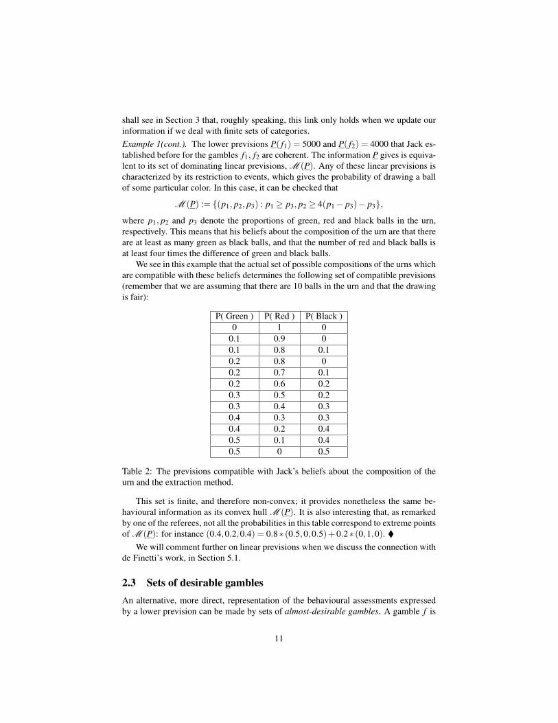
We see in this example that the actual set of possible compositions of the urns whichare compatible with these beliefs determines the following set of compatible previsions(remember that we are assuming that there are 10 balls in the urn and that the drawingis fair):

P( Green ) P( Red ) P( Black )0 1 0

0.1 0.9 00.1 0.8 0.10.2 0.8 00.2 0.7 0.10.2 0.6 0.20.3 0.5 0.20.3 0.4 0.30.4 0.3 0.30.4 0.2 0.40.5 0.1 0.40.5 0 0.5

Table 2: The previsions compatible with Jack’s beliefs about the composition of theurn and the extraction method.

This set is finite, and therefore non-convex; it provides nonetheless the same be-havioural information as its convex hull M (P). It is also interesting that, as remarkedby one of the referees, not all the probabilities in this table correspond to extreme pointsof M (P): for instance (0.4,0.2,0.4) = 0.8∗ (0.5,0,0.5)+0.2∗ (0,1,0).

We will comment further on linear previsions when we discuss the connection withde Finetti’s work, in Section 5.1.

2.3 Sets of desirable gamblesAn alternative, more direct, representation of the behavioural assessments expressedby a lower prevision can be made by sets of almost-desirable gambles. A gamble f is

11

said to be almost-desirable when our subject is almost disposed to accept it, meaningthat he considers the gamble f + ε to be desirable for every ε > 0 (although nothing issaid about the desirability of f ).

Following the behavioural interpretation we gave in Section 2.1 to lower previsions,we see that the gamble f −P( f ) must be almost-desirable for our subject: if P( f ) ishis supremum acceptable buying price, then he must accept the gamble f −P( f )+ ε ,which means paying P( f )− ε for the gamble f , for every ε > 0. The lower previsionof f is the maximum value of µ such that the gamble f −µ is almost-desirable to oursubject.

We can also express the requirement of coherence in terms of sets of almost-desirable gambles. Assume that, out of the gambles in L (Ω), our subject judges thegambles in D to be almost-desirable. His assessments are coherent, and we say that Dis coherent, if and only if the following conditions hold:

(D0) If f ∈D , then sup f ≥ 0 [avoiding sure loss].

(D1) If inf f > 0, then f ∈D [accepting sure gains].

(D2) If f ∈D ,λ > 0, then λ f ∈D [positive homogeneity].

(D3) If f ,g ∈D , then f +g ∈D [addition].

(D4) If f +δ ∈D for all δ > 0, then f ∈D [closure].

Let us give an interpretation of these axioms. D0 states that a gamble f whichmakes him lose utiles, no matter the outcome, should not be acceptable for our subject.D1 on the other hand tells that he should accept a gamble which will always increasehis wealth. D2 means that the almost-desirability of a gamble f should not dependon the scale of utility we are considering. D3 states that if two gambles f and g arealmost-desirable, our subject should be disposed to accept their combined transaction.Axioms D0-D3 characterize the so-called desirable gambles (see [71, Section 2.2.4]).A class of desirable gambles is always a convex cone of gambles. Axiom D4 is aclosure property, and allows us to give an interpretation in terms of almost-desirability.

It is a consequence of axioms (D1) and (D4) that any non-negative gamble f isalmost-desirable. From this and (D3), we can deduce that if a gamble f dominates analmost-desirable gamble g, then f (which is the sum of the almost-desirable gambles gand f−g) is also almost-desirable. Finally, it follows from (D2) and (D3) that a positivelinear combination of almost-desirable gambles is also almost-desirable. These are therationality requirements we have used in Section 2.1 to justify the notion of coherence.

A coherent set of almost-desirable gambles is a closed convex cone containing allnon-negative gambles and not containing any uniformly negative gambles. There is,moreover, a one-to-one correspondence between coherent lower previsions on L (Ω)and coherent sets of almost-desirable gambles: given a coherent lower prevision P onL (Ω), the class

DP := f ∈L (Ω) : P( f )≥ 0 (4)

is a coherent set of almost-desirable gambles. Conversely, if D is a coherent set ofalmost-desirable gambles, the lower prevision PD given by

PD ( f ) := maxµ : f −µ ∈D (5)

12

is coherent. Moreover, it can be checked that the operations given in Equations (4) and(5) commute, meaning that if we consider a coherent lower prevision P on L (Ω) andthe set DP of almost-desirable gambles that we can obtain from it via Equation (4),then the lower prevision PDP

that we define on L (Ω) by Equation (5) coincides withP; and similarly if we start with a set of almost-desirable gambles.

Since the assessments expressed by means of a coherent lower prevision P canalso be expressed by means of its set of dominating linear previsions M (P), we seethat this set is also equivalent to the set of almost-desirable gambles D we have justderived. Indeed, given a coherent set of almost-desirable gambles D , we can considerthe set of linear previsions

MD := P ∈ P(Ω) : P( f )≥ 0 for all f in D.

MD is a closed and convex set of linear previsions, and its lower envelope P coincideswith the coherent lower prevision induced by D through Equation (5).

Conversely, given a closed and convex set of linear previsions M , we can considerthe set of gambles

DM = f ∈L (Ω) : P( f )≥ 0 for all P in M .

DM is a coherent set of almost-desirable gambles, and the lower prevision PDMit

induces is equal to the lower envelope of M .

Example 1(cont.). From the set of linear previsions M (P) compatible with Jack’s co-herent assessments, we obtain the class of almost-desirable gambles

D = (a1,a2,a3) :a1 +a3 ≥ 0, a2 ≥ 0, a1 ≥max−4a2,−3(a1 +a2 +a3),−a2−4(a1 +a3),

where a1 = f (green),a2 = f (red),a3 = f (black).

Hence, we have three equivalent representations of coherent assessments: coher-ent lower previsions, closed and convex sets of linear previsions, and coherent sets ofalmost-desirable gambles. The use of one or another of these representations will de-pend on the context: for instance, a representation in terms of sets of linear previsionsmay be more useful if we want to give our model a Bayesian sensitivity analysis inter-pretation, while the use of sets of almost-desirable gambles may be more interesting inconnection when decision making.

Note however that these representations do not tell us anything about our subject’sbuying behavior for the gambles f at the price P( f ): he may accept it, as he does forthe price P( f )− ε for all ε > 0, but then he also might not. If we want to give infor-mation about the behavior for P( f ), we have to consider a more informative model:sets of really desirable gambles. These sets allow to distinguish between desirabilityand almost desirability, and they solve moreover some of the difficulties we shall seein Section 3 when talking about conditioning on sets of probability zero [77]. We referto [71, Appendix F], [77] and [20] for a more detailed account of this more generalmodel.

13

2.4 Natural extensionAssume now that our subject has established his acceptable buying prices rates for allgambles on some domain K . He may then wish to check which are the consequencesof these assessments for other gambles. If for instance he is disposed to pay a price µ1for a gamble f1 and a price µ2 for a gamble f2, he should be disposed to pay at leastthe price µ1 + µ2 for their sum f1 + f2. In general, given a gamble f which is not inthe domain, he would like to know which is the supremum buying price that he shouldfind acceptable for f , taking into account his previous assessments (P), and using onlythe condition of coherence.

Assume that for a given price µ there exist gambles g1, . . . ,gn in K and non-negative real numbers λ1, . . . ,λn, such that

f (ω)−µ ≥n

∑i=1

λi(gi(ω)−P(gi)).

Since all the transactions in the sum of the right-hand side are acceptable to him, soshould be the left-hand side, which dominates their sum. Hence, he should be disposedto pay the price µ for the gamble f , and therefore his supremum acceptable buyingprice should be greater than or equal to µ . To use the language of the previous section,the right-hand side of the inequality is an almost-desirable gamble, and as a conse-quence so must be the gamble on the left-hand side. And the correspondence betweenalmost-desirable gambles and coherent lower previsions implies then that the lowerprevision of f should be greater than, or equal to, µ .

The lower prevision that provides these supremum acceptable buying prices iscalled the natural extension of P. It is given, for f ∈L (Ω), by

E( f ) = supgi∈K ,λi≥0,

i=1,...,ni,ni∈N

infω∈Ω

f (ω)−

n

∑i=1

λi[gi(ω)−P(gi)]

. (6)

The reasoning above tells us that our subject should be disposed to pay the price E( f )−ε for the gamble f , and this for every ε > 0. Hence, his supremum acceptable buyingprice should dominate E( f ). But we can check also that this value is sufficient toachieve coherence ([71, Theorem 3.1.2]).

Therefore, E( f ) is the smallest, or more conservative, value we can give to thebuying price of f in order to achieve coherence with the assessments in P. There maybe other coherent extensions, which may be interesting in some situations; however,any other of these less conservative, coherent extensions will represent stronger assess-ments than the ones that can be derived purely from P and the notion of coherence.This is why we usually adopt E as our inferred model.

Coherent lower previsions constitute a very general model for uncertainty: theyinclude for instance as particular cases 2- and n-monotone capacities, belief functions,or probability measures. In this style, the procedure of natural extension includes asparticular cases many of the extension procedures present in the literature: Choquetintegration of 2- and n-monotone capacities, Lebesgue integration of probability mea-sures, or Bayes’s rule for updating probability measures. It provides the consequences

14

for other gambles of our previous assessments and the notion of coherence. If for in-stance we consider a probability measure on some σ -field of events A , the naturalextension to all events will determine the set of finitely additive extensions of P toP(Ω), and it will be equal to the lower envelope of this set. It coincides moreoverwith the inner measure of P.

Example 1(cont.). Jack is offered next a new gamble f3, whose reward is 2000 euros ifhe draws a green ball, 3000 if he draws a red ball, and 4000 euros if he draws a blackball. Taking into account his previous assessments, P( f1) = 5000, P( f2) = 4000, heshould at least pay

E( f3)

= supλ1,λ2≥0

min2000−5000λ1+4000λ2,3000−1000λ2,4000+5000λ1−5000λ2.

It can be checked that this supremum is achieved for λ1 = 0,λ2 = 0.2. We obtain thenE( f3) = 2800. This is the supremum acceptable buying price for f3 that Jack can derivefrom his previous assessments and the notion of coherence.

If the lower prevision P does not avoid sure loss, then Equation (6) yields E( f ) =∞

for all f ∈L (Ω). The idea is that if our subject’s initial assessments are such that hecan end up losing utiles no matter the outcome of the experiment, he will also loseutiles with any other gamble that they offer to him. Because of this, the first thing wehave to verify is whether the initial assessments avoid sure loss, and only then we canconsider their consequences on other gambles.

When P avoids sure loss, E is the smallest coherent lower prevision on all gamblesthat dominates P on K , in the sense that E is coherent and any other coherent lowerprevision E ′ on L (Ω) such that E ′( f ) ≥ P( f ) for all f ∈ K will satisfy E ′( f ) ≥E( f ) for all f in L (Ω). E is not in general an extension of P; it will only be sowhen P is coherent itself. Otherwise, the natural extension will correct the assessmentspresent in P into the smallest possible coherent lower prevision. Hence, the notion ofnatural extension can be used to modify the initial assessments into other assessmentsthat satisfy the notion of coherence, and it does so in the least-committal way, i.e., itprovides the smallest coherent lower prevision with the same property.

Example 1(cont.). Let us consider again the assessments P( f1) = 5000,P( f2) = 4000and P( f2) = 6000. These imply the acceptable buying transactions in Table 1, which,as we showed, avoid sure loss but are incoherent. If we apply Equation (6) to themwe obtain that their natural extension is E( f1) = 5000,E( f2) = 4000,E( f2) = 5000.Hence, it is a consequence of coherence that Jack should be disposed to sell the gamblef2 for anything bigger than 5000 euros.

The natural extension of the assessments given by a coherent lower prevision Pcan also be calculated in terms of the equivalent representations we have given in Sec-tions 2.2 and 2.3.

Consider a coherent lower prevision P with domain K , and let DP be the set ofalmost-desirable gambles associated with the lower prevision P by Equation (4):

DP := f ∈K : P( f )≥ 0.

15

The natural extension EDP of DP provides the smallest set of almost-desirable gamblesthat contains DP and is coherent. It is the closure (in the supremum norm topology) of

f : ∃ f j ∈DP,λ j > 0 such that f ≥n

∑j=1

λ j f j, (7)

which is the smallest convex cone that contains DP and all non-negative gambles. Thenthe natural extension of P to all gambles is given by

E( f ) = supµ : f −µ ∈ EDP.

If we consider the set M (P) of linear previsions that dominate P on K , then

E( f ) = minP( f ) : P ∈M (P). (8)

This last expression also makes sense if we consider the Bayesian sensitivity analysisinterpretation we have given to coherent lower previsions in Section 2.2: there is alinear prevision modelling our subject’s information, but his imperfect knowledge of itmakes him consider a set of linear previsions M (P), whose lower envelope is P. If hewants to extend P to a bigger domain, he should consider all the linear previsions inM (P) as possible models (he has no additional information allowing to disregard anyof them), or equivalently their lower envelope. He obtains then that M (P) = M (E).

The procedure of natural extension preserves the equivalence between the differ-ent representations of our assessments: if we consider for instance a coherent lowerprevision P with K and the set of almost-desirable gambles DP we derive from Equa-tion (4), then we can consider the natural extension of DP via Equation (7). The co-herent lower prevision we can derive from this set of acceptable gambles using Equa-tion (5) coincides with the natural extension E of P. This is because the notion ofnatural extension, both for lower or linear previsions or for sets of desirable gamblesdetermines the least-committal extension of our initial model that satisfies the notionof coherence.

On the other hand, we can also consider the natural extension of a lower previsionP from a domain K to a bigger domain K1 (not necessarily equal to L (Ω)). It canbe checked then that the procedure of natural extension is transitive, in the followingsense: if E1 denotes the natural extension of P to K1 and we later consider the naturalextension E2 of E1 to some bigger domain K2 ⊃K1, then E2 agrees with the naturalextension of P from K to K2: in both cases we are only considering the behaviouralconsequences of the assessments on K and the condition of coherence. This is easiestto see using Equation (8): we have M (E1) = M (E2) = M (P).

3 Updating and combining informationSo far, we have assumed that the only information that our subject possesses about theoutcome of the experiment is that it belongs to the set Ω. But it may happen that, afterhe has made his assessments, he comes to have some additional information about thisoutcome, for instance that it belongs to some element of a partition B of Ω. He thenhas to update his assessments, and the way to do this is by means of what we shall callconditional lower previsions.

16

3.1 Conditional lower previsionsLet B be a subset of the sampling space Ω, and consider a gamble f on Ω. Walley’stheory of coherent lower previsions gives two different interpretations of P( f |B): theupdated and the contingent one. The most natural in our view is the contingent in-terpretation, under which P( f |B) is our subject’s current supremum buying price forthe gamble f contingent on B, that is, the supremum value of µ such that the gambleIB( f −µ) is desirable for our subject.

In order to relate our subject’s current dispositions on a gamble f contingent onB with his dispositions towards this gamble if he later shall come to know whetherthe outcome of the experiment belongs to B, Walley introduces the so-called updatingprinciple. We say a gamble f is B-desirable for our subject when he is currently dis-posed to accept f provided he later observes that the outcome belongs to B. Then theupdating principle requires that a gamble is B-desirable if and only if IB f is desirable.In this way, we can relate the current and future dispositions of our subject.

Under the updated interpretation of conditional lower previsions, P( f |B) is the sub-ject’s supremum acceptable buying price he would pay for the gamble f now if he cameto know later that the outcome belongs to the set B, and nothing more. It coincides withthe value determined by the contingent interpretation of P( f |B) because of the updatingprinciple.

Let B be a partition of our sampling space, Ω, and consider an element B of thispartition. This partition could be for instance a class of categories of the set of out-comes. Assume that our subject has given conditional assessments P( f |B) for all gam-bles f on some domain HB. As it was the case for (unconditional) lower previsions,we should require that these assessments are consistent with each other. We say thatthe conditional lower prevision P(·|B) is separately coherent when the following twoconditions are satisfied:

(SC1) It is coherent as an unconditional prevision, i.e.,

supω∈Ω

n

∑i=1

[ fi(ω)−P( fi|B)]−m[ f0(ω)−P( f0|B)]≥ 0 (9)

for all non-negative integers n,m and all gambles f0, . . . , fn in HB;

(SC2) the indicator function of B belongs to HB and P satisfies P(B|B) = 1.

The coherence requirement (9) can be given a behavioural interpretation in thesame way as with (unconditional) coherence in Equation (1): if it does not hold forsome non-negative integers n,m and gambles f0, . . . , fn in HB, then it can be checkedthat either: (i) the almost-desirable gamble ∑

ni=1[ fi−P( fi|B)] incurs in a sure loss (if

m = 0) or (ii) we can raise P( f0|B) in some positive quantity δ , contradicting ourinterpretation of it as his supremum acceptable buying price (if m > 0).

On the other hand, Equation (9) already implies that P(B|B) should be smaller than,or equal to, 1. That we require it to be equal to one means just that our subject shouldbet at all odds on the occurrence of the event B after having observed it.

In this way, we can obtain separately coherent conditional lower previsions P(·|B)with domains HB for all events B in the partition B. It is a consequence of separate

17

coherence that the conditional lower prevision P( f |B) does only depend on the valuesthat f takes on B, i.e, for every two gambles f and g such that f (ω) = g(ω) for allω ∈ B, we should have P( f |B) = P(g|B). This property implies that all the domainsHB can be extended to the common domain H := f = ∑B∈B fB : fB ∈HB ∀B, andwe can define on H a conditional lower prevision P(·|B) by

P( f |B) := ∑B∈B

IBP( f |B),

i.e., the gamble on Ω that assumes the value P( f |B) on all elements of B. This con-ditional lower prevision is then called separately coherent when P(·|B) is separatelycoherent for all B ∈B. It provides the updated supremum buying price after learningthat the outcome of the experiment belongs to some particular element of B. We shalllater use the notation

G( f |B) := IB( f −P( f |B)), G( f |B) := ∑B∈B

G( f |B) = f −P( f |B). (10)

When the domain H of P(·|B) is a linear space containing all constant gambles,then separate coherence is equivalent to:

(C1) P( f |B)≥ infω∈B f (ω).

(C2) P(λ f |B) = λP( f |B).

(C3) P( f +g|B)≥ P( f |B)+P(g|B).

for all positive real λ , B ∈B and gambles f ,g in H . The first requirement shows thatthe conditional lower prevision on B should only depend on the behavior of f on thisset; conditions (C2) and (C3) are the counterparts of the requirements (P2) and (P3) wemade for unconditional lower previsions, respectively.

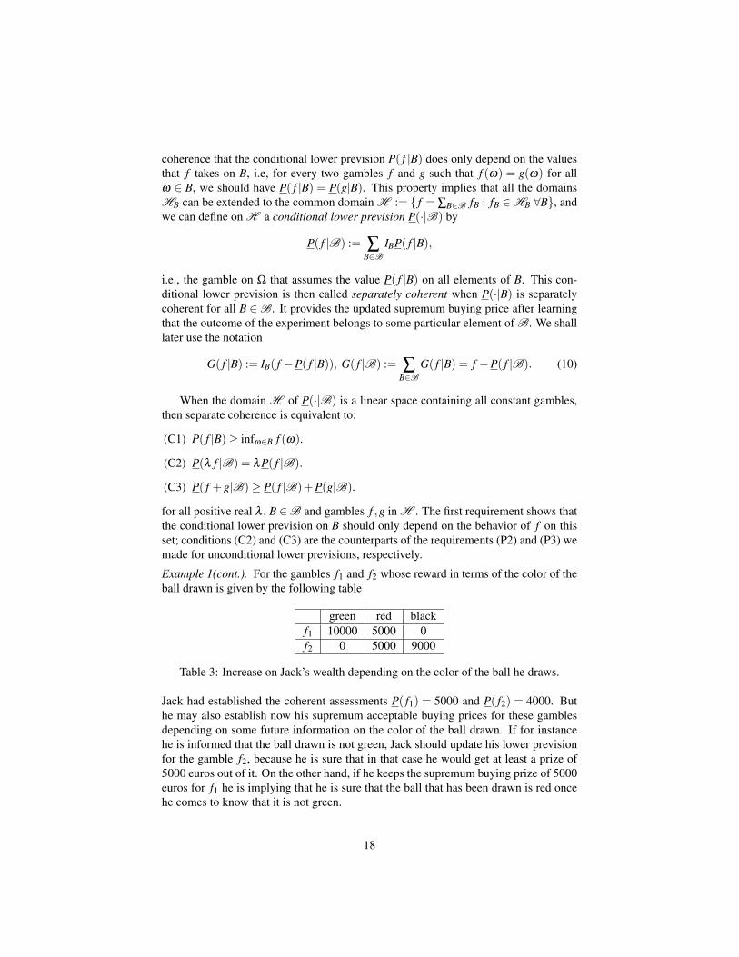
Example 1(cont.). For the gambles f1 and f2 whose reward in terms of the color of theball drawn is given by the following table

green red blackf1 10000 5000 0f2 0 5000 9000

Table 3: Increase on Jack’s wealth depending on the color of the ball he draws.

Jack had established the coherent assessments P( f1) = 5000 and P( f2) = 4000. Buthe may also establish now his supremum acceptable buying prices for these gamblesdepending on some future information on the color of the ball drawn. If for instancehe is informed that the ball drawn is not green, Jack should update his lower previsionfor the gamble f2, because he is sure that in that case he would get at least a prize of5000 euros out of it. On the other hand, if he keeps the supremum buying prize of 5000euros for f1 he is implying that he is sure that the ball that has been drawn is red oncehe comes to know that it is not green.

18

If for instance he considers as possible models the ones in Table 2 and updates themusing Bayes’s rule, then the updated supremum buying prices he should give by takinglower envelopes would be P( f1| not green ) = 0 and P( f2| not green ) = 5000.5

3.2 Coherence of a finite number of conditional lower previsionsIn practice, it is not uncommon to have lower previsions conditional on different parti-tions B1, . . . ,Bn of Ω. We can think for instance of different sets of categories, or ofinformation provided in a sequential way. We end up then with a finite number of con-ditional lower previsions P(·|B1), . . . ,P(·|Bn) with respective domains H1, . . . ,Hn ⊆L (Ω), which we shall assume are separately coherent.

As it was the case with unconditional lower previsions, before making any infer-ence based on these assessments we have to verify that they are consistent with eachother. And again, by ‘consistent’ we shall mean that a combination of acceptable buy-ing prices should neither lead to a sure loss, nor to an increase of the supposedly supre-mum acceptable buying price for a gamble f .

To see which form coherence takes now, we need to introduce the second pillarof Walley’s theory of conditional previsions (the other is the updating principle): theconglomerative principle. This rationality principle requires that if a gamble is B-desirable for every set B in a partition B of Ω, then f is also desirable. Taking intoaccount the updating principle, this means that if IB f is desirable for every B in B, thenf should be desirable.

It follows from this principle that for every gamble f in the domain of P(·|B),the gamble G( f |B) given by Equation (10) should be almost-desirable. This is thebasis of the following definition of coherence. For simplicity, we shall assume thatthe domains H1, . . . ,Hn are linear spaces of gambles. A possible generalization tonon-linear domains can be found in [46]. Given fi ∈Hi, we shall denote by Si( fi) :=B ∈Bi : IB fi 6= 0 the Bi-support of fi. It is the set of elements of Bi where fi is notidentically zero. It follows from the separate coherence of P(·|Bi) that P(0|Bi) = 0 forall i = 1, . . . ,n, and as a consequence the gamble P( f |Bi) (or G( f |Bi), for that matter)is identically zero outside Si( fi).

We say that P(·|B1), . . . ,P(·|Bn) are (jointly) coherent when for all fi ∈Hi, i =1, . . . ,n and all f0 ∈H j,B0 ∈B j for some j ∈ 1, . . . ,n,

supω∈B

[n

∑i=1

G( fi|Bi)−G( f0|B0)

](ω)≥ 0 (11)

for some B ∈ B0∪⋃n

i=1 Si( fi).Assume that Equation (11) does not hold. Then, there is some δ > 0 such that

G( f0|B0)+ IB0δ dominates the almost-desirable gamble ∑ni=1 G( fi|Bi) on every B ∈

B0 ∪⋃n

i=1 Si( fi). As a consequence, the gamble G( f0|B0) + IB0δ should also bealmost-desirable, and this means that P( f |B0)+δ should be an acceptable buying pricefor f , contingent on B0. This is an inconsistency.

5This is an instance of a procedure called regular extension, that can sometimes be used to coherentlyupdate beliefs; see [71, Appendix J] for more details.

19

Remark 1. The sum ∑ni=1 G( fi|Bi)−G( f0|B0)] in the left-hand side in Equation (11)

is identically zero outside the union of the sets in the family B0∪⋃n

i=1 Si( fi). Hence,if in Equation (11) we consider the supremum over all Ω (a condition called weakcoherence by Walley [71, Section 7.1.4]) instead of over the sets in the family B0∪⋃m

i=1 Si( fi), the condition will be automatically satisfied whenever the union of thesesets is not equal to Ω, no matter how inconsistent these assessments are with eachother. This is one of the reasons to consider this stronger version as our definition ofcoherence. See [71, Example 7.3.5] for other undesirable properties of weak coher-ence.

3.2.1 Natural extension of conditional lower previsions

Assume then that our subject has provided a finite number of (separately and jointly)coherent lower previsions P(·|B1), . . . ,P(·|Bn) defined on respective linear subsetsH1, . . . ,Hn of L (Ω). Then he may wish to see which are the behavioural implicationsof these assessments on gambles which are not in the domain. The way to do this isthrough the notion of natural extension. Given f ∈ L (Ω) and B0 ∈Bi, E( f |B0) isdefined as the supremum value of µ for which there are fi ∈Hi such that

supω∈B

[n

∑i=1

G( fi|Bi)− IB0( f −µ)

](ω)< 0 (12)

for all B in the class B0∪∪ni=1Si( fi).

In the particular case where we only have an unconditional lower prevision, i.e.,when n = 1 and B1 = Ω, this notion coincides with the unconditional natural exten-sion we introduced in Section 2.4. If we have a number of conditional lower previsionsP(·|B1), . . . ,P(·|Bn), we can calculate their natural extensions E(·|B1), . . . ,E(·|Bn)to all gambles using Equation (12). If the partitions B1, . . . ,Bn are finite, then thesenatural extensions share some of the properties of the unconditional natural extension:

1. They coincide with P(·|B1), . . . ,P(·|Bn) if and only if these conditional lowerprevisions are coherent.

2. They are the smallest coherent extensions of P(·|B1), . . . ,P(·|Bn) to all gambles.

3. They are the lower envelope of a family of coherent conditional linear previsions,Pγ(·|B1), . . . ,Pγ(·|Bn) : γ ∈ Γ.

Hence, when the partitions are finite, the notion of natural extension of a number ofconditional lower prevision also provides us with the consequences of the assessmentspresent on these previsions and the notion of (joint) coherence, to all gambles in thedomain, and it can also be given a Bayesian sensitivity analysis interpretation. This isinteresting for many applications, where we must deal with finite spaces only; however,there are also interesting situations, such as parametric inference, where we must dealwith infinite spaces and where we end up with partitions that have an infinite numberof different elements. In that case, it is easy to see that in order to achieve coherence,P( f |B0) must be at least as large as the supremum µ that satisfies Equation (12) for

20

some fi ∈Hi, i = 1, . . . ,n. However, and unlike the case of finite partitions, we cannotguarantee that these values provide coherent extensions of P(·|B1), . . . ,P(·|Bn) to allgambles: in general these will only be lower bounds of all the coherent extensions.Indeed, when the partitions are infinite, we can have a number of problems:

1. There may be no coherent extensions, and as a consequence the natural exten-sions may not be coherent [71, Sections 6.6.6 and 6.6.7].

2. Even if the smallest coherent extensions exist, they may differ from the naturalextensions, which are not coherent [71, Section 8.1.3].

3. The minimal coherent extensions, and as a consequence also the natural ex-tensions, may not be lower envelopes of coherent linear collections [71, Sec-tions 6.6.9 and 6.6.10].

The natural extensions are the minimal coherent extensions of the lower previsionsP(·|B1),. . . ,P(·|Bn) if and only if they are jointly coherent themselves. But we needsome additional conditions to guarantee the joint coherence of E(·|B1),. . . ,E(·|Bn).One of these conditions is that all the partitions Bi are finite. But even when thepartitions are infinite it may happen that we are able to characterize the minimal co-herent extensions, but they differ from the natural extensions. One of the reasons forthis defective behaviour of the natural extension in the conditional case is the notion ofconglomerability, that we shall treat in detail in the following section, and that becomestrivial in the case where the partitions are finite.

Example 3. An example where the natural extension fails to provide the minimal co-herent extensions is given in [48, Example 1]. Let us consider the possibility spaceΩ =X1×X2, where X1 =X2 = [0,1], and the partition B = Bx1 : x1 ∈X1, whereBx1 := x1×X2. Let K = λπ1 : λ ∈ R and H = gπ2 : g ∈L (X1), where thegamble λπ1 is defined by λπ1(x1,x2) = λx1, and the gamble gπ2 by gπ2(x1,x2) =g(x1)x2. Let us define the linear (and therefore coherent lower) prevision P on K by

P(λπ1) = λ ,

and the conditional linear prevision P(·|B) on H by

P(gπ2|Bx1) = g(x1)

for all x1 in X1. Then it can be checked that P and P(·|B) are coherent. Given thegamble f on Ω, given by

f (x1,x2) =

0 if (x1,x2) = (1− 1

n ,1−1n ) for some n > 0

1 otherwise,

it can be checked that the natural extension E of P, P(·|B) provides E( f ) = 0. How-ever, in this case the smallest coherent extensions M,M(·|B) of P,P(·|B) can be cal-culated, and we obtain M( f ) = 1. The reason for this discrepancy is that E only givesan extension of P which is coherent with P(·|B); if we also want to extend P(·|B) toall gambles the natural extension may not guarantee coherence.

21

This example provides an instance of the marginal extension of a number of con-ditional and unconditional lower previsions. When these previsions are conditioningon a sequence of increasingly finer partitions, the marginal extension can be used todetermine the smallest coherent extensions to all gambles. See [71, Section 6.7.2] and[48] for more information.

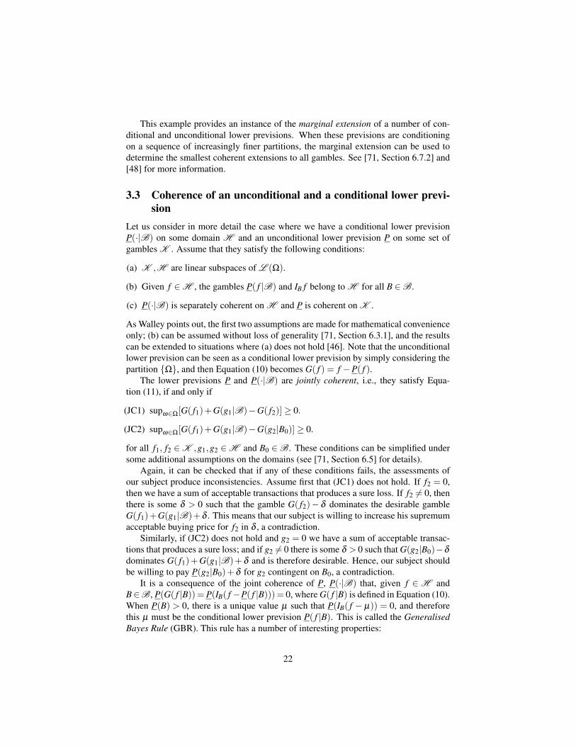
3.3 Coherence of an unconditional and a conditional lower previ-sion

Let us consider in more detail the case where we have a conditional lower previsionP(·|B) on some domain H and an unconditional lower prevision P on some set ofgambles K . Assume that they satisfy the following conditions:

(a) K ,H are linear subspaces of L (Ω).

(b) Given f ∈H , the gambles P( f |B) and IB f belong to H for all B ∈B.

(c) P(·|B) is separately coherent on H and P is coherent on K .

As Walley points out, the first two assumptions are made for mathematical convenienceonly; (b) can be assumed without loss of generality [71, Section 6.3.1], and the resultscan be extended to situations where (a) does not hold [46]. Note that the unconditionallower prevision can be seen as a conditional lower prevision by simply considering thepartition Ω, and then Equation (10) becomes G( f ) = f −P( f ).

The lower previsions P and P(·|B) are jointly coherent, i.e., they satisfy Equa-tion (11), if and only if

(JC1) supω∈Ω[G( f1)+G(g1|B)−G( f2)]≥ 0.

(JC2) supω∈Ω[G( f1)+G(g1|B)−G(g2|B0)]≥ 0.

for all f1, f2 ∈K ,g1,g2 ∈H and B0 ∈B. These conditions can be simplified undersome additional assumptions on the domains (see [71, Section 6.5] for details).

Again, it can be checked that if any of these conditions fails, the assessments ofour subject produce inconsistencies. Assume first that (JC1) does not hold. If f2 = 0,then we have a sum of acceptable transactions that produces a sure loss. If f2 6= 0, thenthere is some δ > 0 such that the gamble G( f2)− δ dominates the desirable gambleG( f1)+G(g1|B)+δ . This means that our subject is willing to increase his supremumacceptable buying price for f2 in δ , a contradiction.

Similarly, if (JC2) does not hold and g2 = 0 we have a sum of acceptable transac-tions that produces a sure loss; and if g2 6= 0 there is some δ > 0 such that G(g2|B0)−δ

dominates G( f1)+G(g1|B)+δ and is therefore desirable. Hence, our subject shouldbe willing to pay P(g2|B0)+δ for g2 contingent on B0, a contradiction.

It is a consequence of the joint coherence of P, P(·|B) that, given f ∈H andB∈B, P(G( f |B)) =P(IB( f −P( f |B))) = 0, where G( f |B) is defined in Equation (10).When P(B) > 0, there is a unique value µ such that P(IB( f − µ)) = 0, and thereforethis µ must be the conditional lower prevision P( f |B). This is called the GeneralisedBayes Rule (GBR). This rule has a number of interesting properties:

22

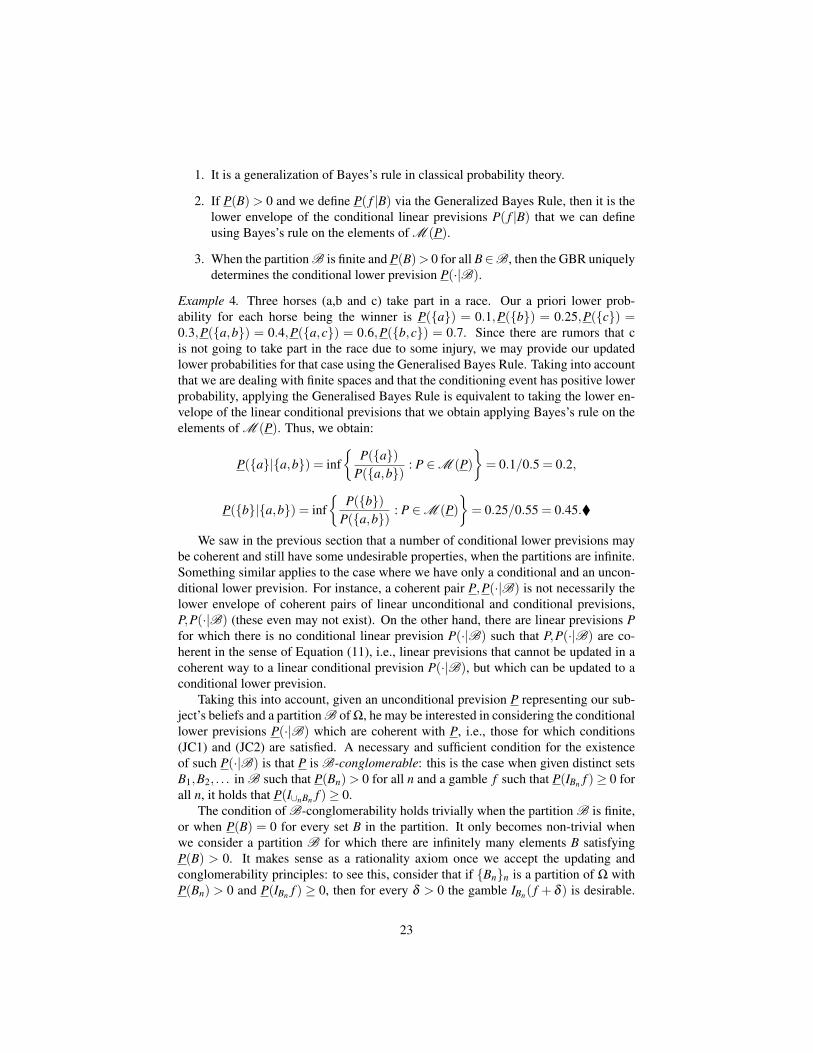
1. It is a generalization of Bayes’s rule in classical probability theory.

2. If P(B)> 0 and we define P( f |B) via the Generalized Bayes Rule, then it is thelower envelope of the conditional linear previsions P( f |B) that we can defineusing Bayes’s rule on the elements of M (P).

3. When the partition B is finite and P(B)> 0 for all B∈B, then the GBR uniquelydetermines the conditional lower prevision P(·|B).

Example 4. Three horses (a,b and c) take part in a race. Our a priori lower prob-ability for each horse being the winner is P(a) = 0.1,P(b) = 0.25,P(c) =0.3,P(a,b) = 0.4,P(a,c) = 0.6,P(b,c) = 0.7. Since there are rumors that cis not going to take part in the race due to some injury, we may provide our updatedlower probabilities for that case using the Generalised Bayes Rule. Taking into accountthat we are dealing with finite spaces and that the conditioning event has positive lowerprobability, applying the Generalised Bayes Rule is equivalent to taking the lower en-velope of the linear conditional previsions that we obtain applying Bayes’s rule on theelements of M (P). Thus, we obtain:

P(a|a,b) = inf

P(a)P(a,b)

: P ∈M (P)= 0.1/0.5 = 0.2,

P(b|a,b) = inf

P(b)P(a,b)

: P ∈M (P)= 0.25/0.55 = 0.45.

We saw in the previous section that a number of conditional lower previsions maybe coherent and still have some undesirable properties, when the partitions are infinite.Something similar applies to the case where we have only a conditional and an uncon-ditional lower prevision. For instance, a coherent pair P,P(·|B) is not necessarily thelower envelope of coherent pairs of linear unconditional and conditional previsions,P,P(·|B) (these even may not exist). On the other hand, there are linear previsions Pfor which there is no conditional linear prevision P(·|B) such that P,P(·|B) are co-herent in the sense of Equation (11), i.e., linear previsions that cannot be updated in acoherent way to a linear conditional prevision P(·|B), but which can be updated to aconditional lower prevision.

Taking this into account, given an unconditional prevision P representing our sub-ject’s beliefs and a partition B of Ω, he may be interested in considering the conditionallower previsions P(·|B) which are coherent with P, i.e., those for which conditions(JC1) and (JC2) are satisfied. A necessary and sufficient condition for the existenceof such P(·|B) is that P is B-conglomerable: this is the case when given distinct setsB1,B2, . . . in B such that P(Bn)> 0 for all n and a gamble f such that P(IBn f )≥ 0 forall n, it holds that P(I∪nBn f )≥ 0.

The condition of B-conglomerability holds trivially when the partition B is finite,or when P(B) = 0 for every set B in the partition. It only becomes non-trivial whenwe consider a partition B for which there are infinitely many elements B satisfyingP(B) > 0. It makes sense as a rationality axiom once we accept the updating andconglomerability principles: to see this, consider that if Bnn is a partition of Ω withP(Bn) > 0 and P(IBn f ) ≥ 0, then for every δ > 0 the gamble IBn( f + δ ) is desirable.

23

The updating and conglomerative principles imply then that f +δ is desirable, whenceP( f +δ )≥ 0. Since this holds for all δ > 0, we deduce that P( f )≥ 0.

More generally, Walley says that a coherent lower prevision P is fully conglomer-able when it is B-conglomerable for every partition B. A full conglomerable coherentlower prevision can be coherently updated to a conditional lower prevision P(·|B) forany partition B of Ω. Again, full conglomerability can be accepted as an axiom ofrationality provided we accept the updating and conglomerability principles, and alsoprovided that when we define our coherent lower prevision we want to be able to up-dated for all possible partitions of our set of values.

There is an important connection between full conglomerability and countableadditivity: given a linear prevision P on L (Ω) taking infinitely many values, it isfully conglomerable if and only for every countable partition Bnn of Ω it satisfies∑n P(Bn) = 1.

Full conglomerability is one of the points of disagreement between Walley’s and deFinetti’s work, that we shall present in more detail in Section 5.1. De Fintetti rejects theassumption of countable additivity on probabilities, and taking into account the aboverelationship also the property of full conglomerability. One key observation here is thatde Finetti does not assume the conglomerative principle as a rationality axiom, and fullconglomerability can be seen as a consequence of it.

When P is B-conglomerable and B ∈B, the conditional lower prevision P( f |B) isuniquely determined by the Generalised Bayes Rule if P(B)> 0. If P(B) = 0, however,there is not a unique value for P( f |B) for which we achieve coherence. The smallestconditional lower prevision P(·|B) which is coherent with P is the vacuous conditionalprevision, given by P( f |B) = infω∈B f (ω), and if we want to have more informativeassessments we may need some additional assumptions. Indeed, the approach to con-ditioning on sets of probability zero is one of the differences in the approach to condi-tioning by Walley (and also by de Finetti and Williams) and that by Kolmogorov. InKolmogorov’s approach, conditioning is made on a σ -field A , and a conditional pre-vision P( f |A ) is any A -measurable gamble which satisfies P(gP( f |A )) = P(g f ) forevery A -measurable gamble g. In particular, if we consider an event B of probabilityzero, Kolmogorov allows the prevision P(·|B) to be completely arbitrary. Walley’s co-herence condition is more general because it can be applied on previsions conditionalon partitions, and is more restrictive when dealing with sets of probability zero thanKolmogorov’s (although it may be argued that it also makes more sense). In particular,for a given linear prevision P there may not exist linear conditional previsions whichare coherent with P.

One interesting approach to conditioning on sets of probability zero in a coherentsetting is the use of zero-layers by Coletti and Scozzafava [8, Chapter 12], which alsoappears in some earlier work by Krauss [38]. Their approach to conditioning is nev-ertheless slightly different from Walley, since they consider conditional previsions asprevisions whose domain is a class of conditional events. See [6, 7, 8] for further infor-mation on Coletti and Scozzafava’s work, and [71, Section 6.10] and [78, Section 1.4]for further details on Walley’s approach to conditioning on events of lower probabilityzero.

24

4 IndependenceNext, we see how we can define the concept of independence in the context of coherentlower previsions. Let us consider two random variables X1,X2 taking values in respec-tive sets X1,X2. In the classical setting, we call the two variables (stochastically)independent when, given the probability measure P that models the value that (X1,X2)assume jointly, any of the following conditions holds6

(a) P(X1 = x1,X2 = x2) = P(X1 = x1) ·P(X2 = x2) for all x1 ∈X1,x2 ∈X2 [decom-position].

(b) P(X1 = x1|X2 = x2) = P(X1 = x1) for all x1 ∈X1,x2 ∈X2 [marginalization].

Remark 2. These two conditions are equivalent provided the marginal distributionsare everywhere non-zero, that is, provided we are not conditioning on sets of probabilityzero. But if P(X2 = x2) = 0 for instance, then condition (a) holds trivially, while thereare many values of P(X1 = x1|X2 = x2) for which condition (b) may not hold, and thiseven under the more restrictive treatment of conditioning of sets of probability zerothat we presented in the previous section. To simplify this section, we shall assumethroughout that the conditioning events have all positive lower probability.

Provided we are conditioning on sets of positive probability, independence is asymmetrical notion: if (b) holds, then we also have

P(X2 = x2|X1 = x1) = P(X2 = x2)

for all x1 ∈X1,x2 ∈X2.When our knowledge about the value that (X1,X2) assume jointly is represented by

means of a coherent lower prevision P on L (X1×X2), there is no unique way ofextending the notion of independence. The properties of decomposition and marginal-ization are no longer equivalent, and moreover symmetry is not immediate anymore,meaning that we must distinguish between irrelevance (an asymmetrical notion) andindependence (its symmetric counterpart). On the other hand, all our definitions mustbe made in terms of variables and not of events, since events do not keep all the infor-mation about the coherent lower prevision P.

In this section, we shall present some of the generalizations proposed in the lit-erature and the relationships between them. To fix things, consider a coherent lowerprevision P on L (X1×X2) representing our knowledge about the value that X1,X2assume jointly. 7 We shall assume throughout that these two variables are logicallyindependent, meaning that the joint variable (X1,X2) can assume any value in the prod-uct space X1×X2. Our information about the random variable X1 is given by themarginal lower prevision P1, where

P1( f ) = P( f )6In this definition we assume that the sets X1,X2 are finite in order to simplify the notation; in the

infinite case we would simply consider density functions instead of probability mass functions. We also useX1 = x1 for denoting the event X−1

1 (x1) to simplify the notation.7Although here we are assuming for simplicity that the domain of P is L (X1×X2), all the developments

we shall make in this section can be generalized to the case where the domain of P is some subset K ofL (X1×X2).

25

for all f ∈L (X1), where f is the gamble given by f (x1,x2) = f (x1) for all (x1,x2)in X1×X2 (such a gamble is called X1-measurable). Similarly, we can express ourinformation about the outcome of X2 by means of a coherent lower prevision P2 onL (X2), given by

P2(g) = P(g)

for all g ∈ L (X2), where g is the gamble given by g(x1,x2) = g(x2) for all (x1,x2)in X1×X2. We shall also assume that we have conditional lower previsions P(·|X1),P(·|X2) on L (X1×X2) such that P,P(·|X1) and P(·|X2) are jointly coherent (i.e., theysatisfy Equation (11)). These conditional lower previsions represent our beliefs aboutthe outcome of one of the experiments provided we observe the outcome of the other.P(·|X1) is a lower prevision conditional on the partition X1 = x1 : x1 ∈X1 of Ω, andsimilarly P(·|X2) is a lower prevision conditional on the partition X2 = x2 : x2 ∈X2of Ω. To simplify the notation we shall sometimes use P(·|x1) to denote P(·|X1 = x1)and P(·|x2) to denote P(·|X2 = x2) for any x1 ∈X1,x2 ∈X2.

In the examples we shall consider in this section we shall deal with finite spacesonly, and the conditioning events shall always have positive lower probability; this willsimplify the calculations of the conditional lower probabilities, because (i) they willbe uniquely determined by the Generalised Bayes Rule and (ii) they will also be thelower envelope of the conditional precise probabilities that can be obtained by applyingBayes’s rule to the set of compatible (precise) models.

4.1 Epistemic irrelevanceThe first generalization of the concept of independence to imprecise probabilities isbased on the marginalization property, and is called epistemic irrelevance. We say thatthe experiment X1 is epistemically irrelevant for X2 when our beliefs about the valuethat X2 takes do not change after we learn the value that X1 has taken. Formally, thisholds if and only if

P( f |X1 = x1) = P2( f )

for all X2-measurable gambles f , and all x1 ∈X1.The notion of epistemic irrelevance can also be defined in terms of sets of linear

previsions [10, 11]: we say that X1 is epistemically irrelevant for X2 when

P2(·|x1) : P2 ∈M (P)= M (P2),

for all x1 in X1, i.e., when learning the outcome about the first experiment does notchange our uncertainty (the set of possible precise models) about the second experi-ment. Similarly, this notion can also be expressed in terms of sets of desirable gam-bles: epistemic irrelevance means that the set of acceptable gambles for X2 should notchange after learning the outcome of X1 [49].

Example 5. We consider three urns with green and red balls. The first urn has one redball and one green ball. In the second urn, we have two green balls, one red ball andtwo other balls of unknown color (they may be red or green). In the third urn, we haveone green ball, two red balls and two other balls of unknown color.

26

We select a ball from the first urn. If it is green, then we select a ball from thesecond urn; if it is red, we select a ball from the third urn. Let X1 be the color of thefirst ball selected and X2 the color of the second ball. We have

P( the second ball is green | the first ball is green) = 2/5P( the second ball is green | the first ball is red) = 1/5,

and thus the first experiment is not epistemically irrelevant to the second.

4.2 Epistemic independenceThe notion of epistemic irrelevance is an asymmetric notion, meaning that X1 can beepistemic irrelevant for X2 while X2 is not epistemic irrelevant for X1. When X1 and X2are epistemically irrelevant to each other, we say that the two experiments are epistem-ically independent. This holds if and only if

P( f |X1 = x1) = P2( f ) and P(g|X2 = x2) = P1(g)

for all X2-measurable gambles f , X1-measurable gambles g, x1 ∈X1, and x2 ∈X2.In terms of sets of linear previsions, the notion of epistemic independence means

that, for every x1 ∈X1 and x2 ∈X2,

P2(·|x1) : P2 ∈M (P)= M (P2) and P1(·|x2) : P1 ∈M (P)= M (P1).

The behavioural interpretation of these definitions is that our sets of desirable gam-bles for either experiment do not change after we learn the outcome of the other exper-iment.

Example 5(cont.). Assume now that in the third urn we also have 2 green balls, 1 redball and 2 balls of unknown color. We have

P( the second ball is green | the first ball is green) = 2/5 andP( the second ball is green | the first ball is red) = 2/5,

and similarly

P( the second ball is red | the first ball is green) = 1/5 andP( the second ball is red | the first ball is red) = 1/5.

Hence, the first variable is epistemically irrelevant for the second. However,

P( the first ball is green | the second ball is green) = 1/3;

(use the composition where we have 2 green balls in the second urn and 4 in the thirdone) while P( the first ball is green ) = 0.5. We conclude that the second variable isnot epistemically irrelevant to the first, and therefore they are not epistemically inde-pendent.

27

This example provides an instance of the phenomena of dilation, where by updatingour beliefs we make them more imprecise. We indeed have

P( the first ball is green | the second ball is green) = 2/3 andP( the first ball is green | the second ball is green) = 1/3,

so knowing the color of the second ball makes our beliefs about the probability ofdrawing a red ball in the first urn change from being precise in 0.5 to belong to theinterval [ 1

3 ,23 ]. See [54] for more information about dilation.

4.3 Independent envelopesAs we said before, in the classical case, if all the marginals are everywhere non-zero,then independence can be expressed equivalently through the decomposition and themarginalization notions. These two properties, however, are no longer equivalent in theimprecise case, and we can have two epistemically independent experiments for whichP(x1,x2) 6= P1(x1) ·P2(x2) for some x1 ∈X1,x2 ∈X2.

The first two notions we have considered are based on extending the marginaliza-tion property to the imprecise case. Next, we introduce two conditions of independencewhich are based on the decomposition property. These conditions are only applied tothe extreme points of the set M (P), because these keep all the information about Pand moreover it can be checked that a decomposition property cannot hold for all theelements of the convex set M (P).

We say that P is an independent envelope when every extreme point P of M (P)factorizes as P = P1×P2, where P1 is the marginal distribution of P on X1 and P2 is themarginal distribution of P on X2. This concept is called independence in the selectionin [10] and type-2 independence in [14].

It is easier to understand the ideas behind this notion if we consider the Bayesiansensitivity analysis interpretation of our beliefs. Assume then that we have two exper-iments X1, X2, and that the probability modelling the first experiment belongs to someset M (P1), while the probability modelling the second experiment belongs to anotherset M (P2). Let M (P) be the set of possible models for the behavior of the two exper-iments, taken together. This set of models can be characterized by its set of extremepoints. Independence in the selection means that each of these extreme points satisfiesthe classical notion of independence, in the sense that it can be written as a product ofits marginals.

Example 5(cont.). Assume now that in the first urn we have one red ball, one greenball and one ball of unknown color, and that in the second and third urns we have twogreen balls, one red ball and two balls of unknown color. Then the variables X1 and X2are epistemically independent: reasoning as in the example in Section 4.2 we deducethat the color of the first ball drawn is irrelevant for the second; conversely, we havethat P( the first ball is green ) = P(the first ball is red ) = 1

3 , and we deduce from thesame example that the color of the second ball is epistemically irrelevant for the first.

Let P be the probability distribution associated with the following composition orthe urns:

28

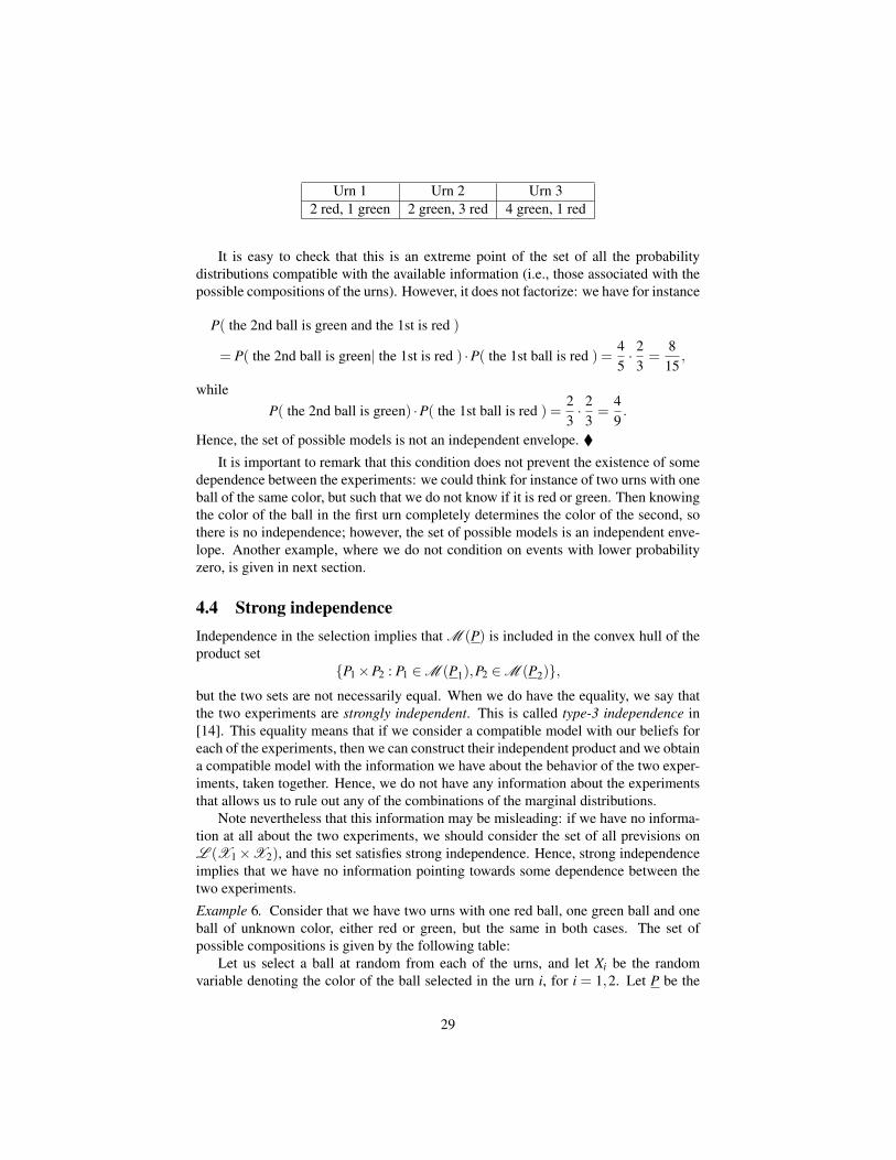
Urn 1 Urn 2 Urn 32 red, 1 green 2 green, 3 red 4 green, 1 red

It is easy to check that this is an extreme point of the set of all the probabilitydistributions compatible with the available information (i.e., those associated with thepossible compositions of the urns). However, it does not factorize: we have for instance

P( the 2nd ball is green and the 1st is red )

= P( the 2nd ball is green| the 1st is red ) ·P( the 1st ball is red ) =45· 2

3=

815

,

whileP( the 2nd ball is green) ·P( the 1st ball is red ) =

23· 2

3=

49.

Hence, the set of possible models is not an independent envelope.

It is important to remark that this condition does not prevent the existence of somedependence between the experiments: we could think for instance of two urns with oneball of the same color, but such that we do not know if it is red or green. Then knowingthe color of the ball in the first urn completely determines the color of the second, sothere is no independence; however, the set of possible models is an independent enve-lope. Another example, where we do not condition on events with lower probabilityzero, is given in next section.

4.4 Strong independenceIndependence in the selection implies that M (P) is included in the convex hull of theproduct set

P1×P2 : P1 ∈M (P1),P2 ∈M (P2),but the two sets are not necessarily equal. When we do have the equality, we say thatthe two experiments are strongly independent. This is called type-3 independence in[14]. This equality means that if we consider a compatible model with our beliefs foreach of the experiments, then we can construct their independent product and we obtaina compatible model with the information we have about the behavior of the two exper-iments, taken together. Hence, we do not have any information about the experimentsthat allows us to rule out any of the combinations of the marginal distributions.

Note nevertheless that this information may be misleading: if we have no informa-tion at all about the two experiments, we should consider the set of all previsions onL (X1×X2), and this set satisfies strong independence. Hence, strong independenceimplies that we have no information pointing towards some dependence between thetwo experiments.

Example 6. Consider that we have two urns with one red ball, one green ball and oneball of unknown color, either red or green, but the same in both cases. The set ofpossible compositions is given by the following table:

Let us select a ball at random from each of the urns, and let Xi be the randomvariable denoting the color of the ball selected in the urn i, for i = 1,2. Let P be the

29

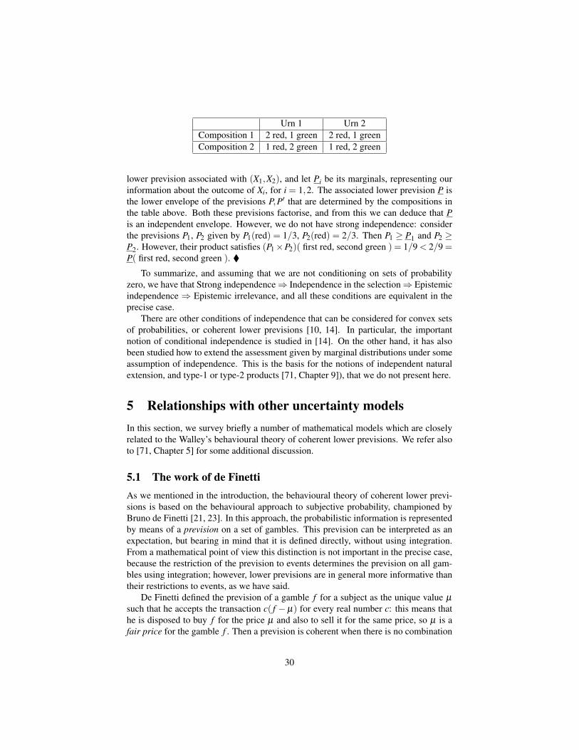
Urn 1 Urn 2Composition 1 2 red, 1 green 2 red, 1 greenComposition 2 1 red, 2 green 1 red, 2 green

lower prevision associated with (X1,X2), and let Pi be its marginals, representing ourinformation about the outcome of Xi, for i = 1,2. The associated lower prevision P isthe lower envelope of the previsions P,P′ that are determined by the compositions inthe table above. Both these previsions factorise, and from this we can deduce that Pis an independent envelope. However, we do not have strong independence: considerthe previsions P1, P2 given by P1(red) = 1/3, P2(red) = 2/3. Then P1 ≥ P1 and P2 ≥P2. However, their product satisfies (P1×P2)( first red, second green ) = 1/9 < 2/9 =P( first red, second green ).

To summarize, and assuming that we are not conditioning on sets of probabilityzero, we have that Strong independence⇒ Independence in the selection⇒ Epistemicindependence ⇒ Epistemic irrelevance, and all these conditions are equivalent in theprecise case.

There are other conditions of independence that can be considered for convex setsof probabilities, or coherent lower previsions [10, 14]. In particular, the importantnotion of conditional independence is studied in [14]. On the other hand, it has alsobeen studied how to extend the assessment given by marginal distributions under someassumption of independence. This is the basis for the notions of independent naturalextension, and type-1 or type-2 products [71, Chapter 9]), that we do not present here.

5 Relationships with other uncertainty modelsIn this section, we survey briefly a number of mathematical models which are closelyrelated to the Walley’s behavioural theory of coherent lower previsions. We refer alsoto [71, Chapter 5] for some additional discussion.

5.1 The work of de FinettiAs we mentioned in the introduction, the behavioural theory of coherent lower previ-sions is based on the behavioural approach to subjective probability, championed byBruno de Finetti [21, 23]. In this approach, the probabilistic information is representedby means of a prevision on a set of gambles. This prevision can be interpreted as anexpectation, but bearing in mind that it is defined directly, without using integration.From a mathematical point of view this distinction is not important in the precise case,because the restriction of the prevision to events determines the prevision on all gam-bles using integration; however, lower previsions are in general more informative thantheir restrictions to events, as we have said.

De Finetti defined the prevision of a gamble f for a subject as the unique value µ

such that he accepts the transaction c( f − µ) for every real number c: this means thathe is disposed to buy f for the price µ and also to sell it for the same price, so µ is afair price for the gamble f . Then a prevision is coherent when there is no combination

30

of acceptable transactions which leads to a sure loss. Mathematically, this is expressedby

supn

∑i=1

λi( fi−P( fi))≥ 0

for every natural number n, real λ1, . . . ,λn and gambles f1, . . . , fn in K . It is easy tosee that this condition is equivalent to the coherence condition we have given in Eq. (2)for linear previsions.

Even if most of de Finetti’s work on coherent previsions can be embedded in Wal-ley’s theory of coherent lower and upper previsions, Walley’s work is not a generaliza-tion of de Finetti’s work, because there are substantial differences between the two:

• The most fundamental one is that Walley does not require our subject to de-termine a fair price for all gambles f in the domain. See [71, Section 5.7] forWalley’s arguments against the assumption of precision.

• Although he did not provide a detailed theory of conditional previsions, his in-terpretation for them is slightly different from Walley’s: he regards them as pre-visions defined on a family of conditional events E|H, where E|H is a logicalentity which is true if both E and H are true, false if H is true and E is false, andvoid if H is false.

• Another difference between the two approaches is their regard towards the con-dition of conglomerability, which is rejected by de Finetti in [23, Section 4.19]:he gives two examples where conglomerability is not satisfied. One argumenthere is that full conglomerability rules out linear previsions which are not count-ably additive (see Section 3.3 for a more precise formulation). The key of thematter, as Walley says in [71, p. 327] is that

“Those who insist on additivity and linearity must either reject con-glomerability or the possibility of extensions to larger domains.”

5.2 The work of WilliamsA first approach to generalizing de Finetti’s work taking into account the presence ofimprecision was considered by Peter Williams in [84, 85, 86] (see also [67] for a recentreview of Williams’ work). It was also motivated by the treatment of conditional pre-visions in de Finetti’s work. Williams defines a coherent conditional lower previsionby means of a set of acceptable gambles, in the sense that P( f |B) is defined as thesupremum value of µ such that IB( f −µ) is an acceptable transaction for our subject.In particular, if we consider B = Ω, P( f |Ω) agrees with Walley’s behavioural interpre-tation of a lower prevision (see [86] for a more detailed account of the unconditionalcase). Similarly, P( f |B) is defined as the infimum value of µ such that the gambleIB(µ − f ) is acceptable for our subject, which in the case of unconditional lower pre-visions (B = Ω) becomes the infimum selling price for f .

31

In order to define coherence, he requires the set of acceptable gambles to satisfyconditions which are slightly weaker than (D0)–(D3).8 He proves then that a necessarycondition for coherence is that

supx∈∪n

i=0Bi

[n

∑i=1

λiIBi( fi−P( fi|Bi))−λ0IB0( f0−P( f0|B0))](x)≥ 0, (13)

for every natural number n, Bi included in Ω, non-negative real λi and fi in the domainof P(·|Bi) for i = 0, . . . ,n. This condition is sufficient if we require the set of acceptablegambles to satisfy (D0)–(D3).

Let us compare this Condition, that we shall call W -coherence, with Walley’s no-tion of coherence for conditional lower previsions (11). We see that, under Walley’sterminology (see Section 3.2), Condition (13) corresponds to the particular case ofEquation (11) where the sets Si( fi) are finite for all i. Hence, if we consider a num-ber of conditional lower previsions P(·|B1), . . . ,P(·|Bn) where B1, . . . ,Bn are finitepartitions of Ω, then they are coherent in the sense of Walley if and only if they areW-coherent. However, for arbitrary (not necessarily finite) partitions B1, . . . ,Bn, Wal-ley’s notion of coherence is stronger than that of Williams.

The use of W-coherence for conditional lower previsions has a number of technicaladvantages over Walley’s condition:

• W-coherent conditional lower previsions are always lower envelopes of sets ofW-coherent conditional linear previsions ([85, Theorem 2], see also [71, Sec-tion 8.1]), and as a consequence they can be given a Bayesian sensitivity analysisinterpretation.

• We can always construct the smallest W-coherent extension of a W-coherentconditional lower prevision [85, Theorem 1]. Moreover, this result can be gen-eralised towards unbounded gambles [63].

There are also, however, a number of drawbacks:

• If we express the condition using Walley’s terminology, it assumes the finite-ness of the sets Si( fi) involved, whereas for many statistical applications it isimportant to consider non-finite spaces and partitions.

• It does not satisfy in general the conglomerability condition, as a consequencewhen we consider infinite partitions we may end up with acceptable transactions(W-coherent) which incur in a sure loss [71, Example 6.6.9].

As a summary, Williams’ definition of coherence is a valid and interesting alter-native to Walley, that avoids some of the drawbacks of Walley’s approach to condi-tional lower previsions. Moreover, it seems to be better suited for extending the theoryto unbounded gambles. The choice between the two is based in whether we acceptfull conglomerability as a rationality requirement, which means essentially that weassume countable additivity of the involved previsions (but without measurability re-quirements): see Section 3.3 and [71, Section 6.9] for more details.

8The difference is that he does not require a gamble f 6= 0 with infx∈supp( f ) f (x) = 0 to be accepted, nora gamble f 6= 0 with supx∈supp( f )(x) = 0 to be rejected, where supp( f ) = ω ∈Ω : f (ω) 6= 0 is the supportof f . This is related also to Walley’s discussion of really desirable gambles [71, Appendix F].

32

5.3 Kuznetsov’s work on interval-valued probabilitiesIn a relatively unknown book on interval valued probabilities [40], the Russian math-ematician V. Kuznetsov established, in parallel to Walley, a theory of interval-valuedprobabilities and previsions which has many things in common with the behaviouraltheory we have presented. Starting from some axioms which are equivalent to Walley,he deduces many of the properties that can also be found in Walley’s book. He also ob-tains some interesting limit results for coherent lower and upper previsions. The maindifferences between both theories are:

• Kuznetsov does not consider the behavioural interpretation for coherent lowerand upper previsions in terms of buying and selling prices.

• He makes some assumptions in the domains, and therefore we cannot considerprevisions with arbitrary domains as is the case with Walley’s theory.

• His theory is valid for unbounded gambles, and the domain of his upper previ-sions contains at least those gambles which are bounded above (and similarly, thedomain of his lower previsions includes at least the gambles which are boundedbelow).

• When conditioning on a set B of lower probability zero and positive upper prob-ability, he suggests taking the limit on conditional dominating previsions, whichgive positive probability to B. This is related to the notion of regular extensionin Walley [71, Appendix K].

See [41, 42] for two short papers in English presenting Kuznetsov’s work, and[12, 66] for some works derived from his theory.

5.4 Weischelberger’s F- and R-probabilitiesRecently, Kurt Weischleberger and some of his colleagues have also established a the-ory of interval-valued probabilities [79, 80, 81] that is more statistically oriented thanWalley’s. This theory considers two non-additive measures L ≤ U determining thelower and upper bounds for our probabilities. The set of (finitely additive) probabili-ties M that lie between L and U are called the structure determined by L,U .

L and U are said to determine an R-probability with structure M when M 6= /0, andan F-probability when L,U are the infimum and the supremum of the probabilities inM , respectively. Hence, these concepts are equivalent to the notions of avoiding sureloss and coherence for imprecise probabilities.

Weischleberger’s theory is more related to the classical works on probability theory,in the sense that it focuses on probabilities instead of previsions and that it also makessome measurability assumptions that are not present in Walley’s theory. Another dif-ference is that Weischelberger’s work does not use a subjective interpretation of lowerand upper probabilities, and it allows to connect the notions of avoiding sure loss andcoherence with a frequentist interpretation of probability (see also [69] for another pa-per in this direction). The treatment of conditional lower and upper probabilities andof the notion of independence is also different [82].

See [2, 82] for some recent work based on this theory.

33

5.5 The Dempster-Shafer theory of evidenceNext, we outline the main features of the Dempster-Shafer theory of evidence [57]. Theorigin of this theory is in Dempster’s work on random sets, or measurable multi-valuedmappings [24, 25].

Let A be a field of subsets of Ω, and consider a lower probability P : A → [0,1]that satisfies P( /0) = 0,P(Ω) = 1. P is said to be completely monotone if it is monotoneand for any events A1, . . . ,An in A and n≥ 2,

P(∪ni=1Ai)≥ ∑

I⊆1,...,n(−1)|I|+1P(∩i∈IAi), (14)

where |I| denotes the cardinality of the set I. A lower probability that satisfies Equa-tion (14) for all k ≤ p is called p-monotone. A complete monotone lower probabilityis then one that is n-monotone for every natural number n. When Ω is a finite space,and the field A is the class of all subsets of Ω, a completely monotone lower proba-bility is called a belief function. A belief function is determined by its so-called basicprobability assignment m, which is given by

m(A) = ∑B⊆A

(−1)|A−B|P(B).

Then P is given, for all A ⊆ X , by P(A) = ∑B⊆A m(B). The upper probability that wecan generate from a completely monotone lower probability using conjugacy is said tobe completely alternating, and, in the particular case where Ω is finite, a plausibilityfunction. The relationship between a plausibility function P and the basic probabilityassignment m of its conjugate belief function P is P(A) = ∑B∩A 6= /0 m(B). The basicprobability assignment of a set A can be interpreted as the measure of belief that iscommitted exactly to A. Then P(A) would be our subject’s belief that the result ofthe experiment belongs to the set A, while P(A) is the measure of his belief that theoutcome of the experiment may belong to A (or, perhaps more clearly, the measure ofbelief that does not rule out that the outcome is in A). This is the so-called evidentialinterpretation.

From the behavioural point of view, multi-valued mappings have been studied in[71, Section 4.3.5] and in [47]. On the other hand, 2- (and in particular completely-)monotone functions were studied by Walley in [68]. Some of his results generalize tothe case where the domain is a lattice of events instead of a field [18]. It can be checked[68] that a 2-monotone lower probability is in particular coherent, and therefore so aren- and completely monotone capacities. More generally, we can consider n-monotonelower previsions, which appeared in [5, Chapter 3] as functionals between an Abeliansemigroup and an Abelian group, and were studied from a behavioural point of view in[17, 18]. Hence, from a static point of view (without considering updating or combi-nation of information) Dempster-Shafer theory can be embedded into Walley’s theoryof coherent lower previsions.

One of the main features of the evidential theory, and Walley’s main point of crit-icism (see [71, Section 5.13] and [74]) is Dempster’s Rule of Combination [24, 57].It is used to combine several belief functions which are based on different sources ofinformation into one belief function. Let P1,P2 be two belief functions with basic

34

probability assignments m1,m2, respectively. The combined belief function P is theone related to the basic probability assignment

m(C) = ∑A∩B=C

m1(A)m2(B), (15)

where, if necessary, we normalize it by multiplying by[1− ∑

A∩B= /0m1(A)m2(B)

]−1

,

which is a measure of the extent of the conflict between P1 and P2.This rule of combination is only reasonable for Walley provided we make some ad-

ditional assumptions on the relationship between the experiments that underlie P1,P2([71, Section 5.13.7]). In particular, the conditioning rule that we may derive from itmay fail to produce conditional lower previsions which are coherent with the uncondi-tional ones. We may have to make some extra assumptions of conditional independenceif we want it to satisfy coherence, and this requirement may be unreasonable in somecases. See also [44, 50, 87] for further criticism of this rule.

5.6 The game-theoretic approach to imprecise probabilitiesWe would like to conclude this section by making a brief summary of recent work byShafer and Vovk [59], where a connection is established between probability and fi-nance through a game-theoretic approach to coherent lower previsions. The ideas ofthis approach are roughly similar to the ones behind the behavioural theory we haveoutlined: we also have here acceptable transactions and study whether they can lead toa sure loss. There are, however, a number of important differences between the two:Shafer and Vovk consider a game between two players, whereas Walley’s theory is fo-cused on one subject who establishes buying and selling prices;9 there is no assumptionof boundedness of the variables involved; and they focus on the consequences and notso much on probability.

Let us make a short summary of the main ideas in this work. We refer to [60, 59]for more details. Consider a game between two players, called World and Skeptic, whoplay according to a certain protocol. The first player (World) can make a number ofmoves, where the next move may depend on his previous moves, but not on the onesmade by Skeptic. These moves can be represented in a tree, and we call a situationsome connected path in the tree that starts at the root of the tree.

In each situation t, Skeptic has a number of possible moves, and a gain functionassociated with the move he makes and World’s next move, representing the change inSkeptic capital associated with these two moves. A strategy is then a function deter-mining Skeptic next move for each non-final situation in the tree representing World’smoves, and the associated capital if he starts the game with zero capital is his capitalprocess.

9A two player model is already present in [61].

35

Under this interpretation, Shafer and Vovk define upper and lower prices for realvariables. The upper price for a variable f in a non-final situation t is the lowest priceat which Skeptic can buy the variable f at the end of the game, no matter what movesWorld makes, using some strategy. The lower price for a variable f in a non-finalsituation t can be given an analogous interpretation using conjugacy.

A gambling protocol is called a probability protocol when the following two con-ditions are satisfied:

(PP1) The set of possible moves for Skeptic in any situation t is a convex cone.

(PP2) For each non-final situation, Skeptic’s gain function is linear with respect toSkeptic’s moves, for any move of World fixed.

It is called coherent when for each non-final situation and each possible move s ofSkeptic there is another move w of World such that the gain associated with (s,w) isnon-positive.

For many of their developments Shafer and Vovk decompose World into multipleplayers. They consider for instance Reality and Forecaster, where Forecaster deter-mines for each non-final situation the set of possible moves and the gain function forSkeptic, while Reality determines the move of World. Shafer and Vovk establish anumber of limit results, such as weak and strong laws of large numbers, for coherentprobability protocols.

Under the terminology we have considered throughout this survey, our subjectwould take the role of Forecaster, in the sense that he establishes the supremum buyingprices for all gambles in the domain. Then, we check the coherence of these pricesusing the roles of Skeptic (selecting some gambles in the domain) and Reality (deter-mining the outcome of the experiment, that is, the value ω in Ω). Walley’s notion ofcoherence means that the buying prices established by Forecaster should not be ex-ploitable by Skeptic in order to assure himself a gain, no matter how World moves.

We see then that, although some of the concepts used by Shafer and Vovk aresimilar to the ones in Walley’s theory of coherent lower previsions (the behaviouralinterpretation, the notion of coherence, etc), there are also differences between the twoapproaches, like the use of two players and the extension to unbounded gambles. Itis therefore interesting that Shafer and Vovk’s work on coherent probability protocolshas been recently connected to Walley’s theory of coherent lower previsions in [19]. Ithas been proven that for every coherent probability protocol there exists an immediateprediction model such that both lead to identical buying prices, and vice versa. See[19] for more information. In this sense, in spite of some of their differences, theresults from one theory can be embedded into the other.10

6 ApplicationsLet us give some comments now on the use of the theory of coherent lower previsionsin other contexts. Since the origins of subjective probability are in decision making, it

10The (possible) unboundedness of the variables in the models is overcome in the case of coherent lowerprevisions by working with sets of (really) desirable gambles, instead of almost-desirable ones ([19, Sec-tions 3 and 4]).

36

is not really surprising that much of the work made on practical uses of coherent lowerprevisions, which stem from subjective probability theory, is related to decision theory.Indeed, imprecise probabilities can be seen as a more realistic model for practical deci-sion problems, because they allow us to treat some of the most common problems thatappear in practice: lack of available information, conflicting sources of beliefs, anddifficulties in eliciting expert’s opinions.

The theory of coherent lower previsions, in different forms, has been employed in anumber of applications, in different frameworks such as the environmental [70] or thebio-medical [64, 72, 90]. One of the consequences of the use of sets of probabilitieswill be that sometimes we cannot decide which of two alternatives must be preferred,something which is to be expected on the other hand in the case of little information.Another feature is that there are many possible ways of generalizing the principle ofmaximum expected utility to coherent lower previsions, such as E-admissibility, inter-val dominance, Γ-maximinity and maximality, etc. We refer to [65] for an overview ofthe different criteria, and to [56] for a comparison of E-admissibility and Γ-maximinity.

There have also been several studies connecting the behavioural theory of coherentlower previsions with different aspects of statistics [73, 75]. One of the most importantis the work in [73], where Walley defined the so-called Imprecise Dirichlet Model.This is a model for inference which relates past and future observations about somevariables. See also [3, 76] for additional information about this model. The ImpreciseDirichlet Model has been applied in different contexts, such as classification [1, 91, 90],reliability analysis [9] or game theory [52]. See also [16, 89] for further theoreticaldevelopments on this subject.

Finally, coherent lower previsions have also been used for dealing with uncertaintyscenarios in climate change [39] and forestry [28].

7 Strengths and challengesThe results mentioned in this paper constitute an attempt to overview the main featuresof the behavioural theory of coherent lower previsions. As a summary, the main virtuesof this theory are:

1. It is better suited for situations where the available information does not justifythe use of a precise probability distribution.

2. It encompasses most of the other generalizations considered in the literature (be-lief functions, 2-monotone capacities, coherent lower probabilities). This is donemainly in two ways:

• By focusing on the behavior towards variables (gambles), and therefore onthe notion of expectation, without going through the behavior on eventsfirst.

• By moving away from the measurability requirements on classical proba-bility theory and considering previsions for arbitrary sets of gambles.

37

3. It provides a behavioural interpretation that leads naturally to decision making,and it can at the same time be given a sensitivity analysis representation in somecases.

Nevertheless, the theory of coherent lower previsions has a number of challengesthat need to be studied in more detail:

1. The concept of coherence, although a reasonable rationality requirement, maybe too weak to produce informative inferences.

2. The theory is established for bounded random variables, or gambles, and thegeneralization towards unbounded random variables is not straightforward.

3. It assumes the linearity of the utility scale, something which may not be reason-able in practice.11

4. Walley’s notion of natural extension of conditional lower previsions has someundesirable properties, which do not seem to be resolvable without giving up onconglomerability.

5. Computing with coherent lower previsions in practice means often solving non-linear problems, whence for big problems the computational costs may be high.

6. There have been until now relatively few applications, and more are needed inorder to effectively compare the applicability of this theory with classical tools.

7. More generally, we need to develop tools to be able to compare the effectivenessof precise and imprecise approaches in a number of situations.

8. There are several notions of independence as well as different optimality criteria,and it is not always clear which of them is better suited for each situation.

9. From the theoretical point of view there are a number of notions and results fromclassical probability theory which have not been generalized, such as ergodictheorems.

These problems constitute the main avenues for future research in the theory.

AcknowledgementsI would like also to express my gratitude to Gert de Cooman, Marco Zaffalon, RomanEffremov and the anonymous referees for some very helpful comments that improvedsubstantially earlier versions of this paper. I also acknowledge the financial support ofthe projects MTM2004-01269 and TSI2004-06801-C04-01.

11But see [51] for an interesting solution to this problem.

38

References[1] A. Antonucci, A. Salvetti, and M. Zaffalon. Credal networks for hazard assess-

ment of debris flows. In J. Kropp and J. Scheffran, editors, Advanced Methodsfor Decision Making and Risk Management in Sustainability Science, pages 237–256. Nova Science, 2007.

[2] T. Augustin and F. Coolen. Non parametric predictive inference and intervalprobability. Journal of Statitical Planning and Inference, 124:251-272, 2004.

[3] J. M. Bernard. An introduction to the imprecise Dirichlet model for inferencewith multinomial data. International Journal of Approximate Reasoning, 39(2–3):123–150, 2005.

[4] E. Borel. Probabilities and life. Dover, New York, 1962.

[5] G. Choquet. Theory of capacities. Annales de l’Institut Fourier. Universite deGrenoble, 5:131–295, 1953.

[6] G. Coletti. Coherent numerical and ordinal probability assessments. IEEE Trans-actions on Systems, Man and Cybernetics, 24:1747–1754, 1994.

[7] G. Coletti and R. Scozzafava. Zero probabilities in stochastic independence. InR.R. Yager, B. Bouchon-Meunier and L.A. Zadeh, editors, Information, Uncer-tainty, Fusion, pages 185–196. Kluwer, 2000.

[8] G. Coletti and R. Scozzafava. Probabilistic logic in a coherent setting. Kluwer,New York, 2002.

[9] F. Coolen. An imprecise Dirichlet model for Bayesian analysis of failure dataincluding right-censored observations. Reliability Engineering and System Safety,56:61–68, 1997.

[10] I. Couso, S. Moral, and P. Walley. A survey of concepts of independence forimprecise probabilities. Risk, Decision and Policy, 5(2):165–181, 2000.

[11] F. Cozman. Irrelevance and independence relations in Quasi-Bayesian networks.In G.F. Coopen and S. Moral, editors, Proceedings of the 14th conference onUncertainty in Artificial Intelligence, pages 89–96, 1998.

[12] F. Cozman. Constructing sets of probability measures through Kuznetsov’s in-dependence condition. In Proceedings of the 2nd International Symposium onImprecise Probabilities and Their Applications, pages 104–111, 2001.

[13] F. Cozman and P. Walley. Graphoid properties of epistemic irrelevance and inde-pendence. Annals of Mathematics and Artificial Intelligence, 45(1–2):173–195,2005.

[14] L. M. de Campos and S. Moral. Independence concepts for convex sets of prob-abilities. In Proceedings of 11th Conference on Uncertainty in Artificial Intelli-gence, pages 108–115, 1995.

39

[15] G. de Cooman. Possibility theory I-III. International Journal of General Systems,25(4):291–371, 1997.

[16] G. de Cooman and M. Zaffalon. Updating beliefs with incomplete observations.Artificial Intelligence, 159(1–2):75–125, 2004.

[17] G. de Cooman, M. C. M. Troffaes, and E. Miranda. n-Monotone lower previ-sions and lower integrals. In Proceedings of the 4th International Symposium onImprecise Probabilities and Their Applications, pages 145–154. 2005.

[18] G. de Cooman, M. C. M. Troffaes, and E. Miranda. n-Monotone lower previsions.Journal of Intelligent and Fuzzy Systems, 16(4):253–263, 2005.

[19] G. de Cooman and F. Hermans. On coherent immediate prediction: connectingtwo theories of imprecise probability. In Proceedings of the 5th InternationalSymposium on Imprecise Probabilities and Their Applications, pages 97–106,2007.

[20] G. de Cooman and E. Miranda. Symmetry of models versus models of symmetry.In W. L. Harper and G. R. Wheeler, editors, Probability and Inference: Essays inHonor of Henry E. Kyburg, Jr., pages 67–149. King’s College Publications, 2007.

[21] B. de Finetti. La prevision: ses lois logiques, ses sources subjectives. Annales del’Institut Henri Poincare, 7:1–68, 1937.

[22] B. de Finetti. Teoria delle Probabilita. Einaudi, Turin, 1970.

[23] B. de Finetti. Theory of probability. John Wiley and Sons, Chichester, 1974–1975. English translation of [22].

[24] A. P. Dempster. Upper and lower probabilities induced by a multivalued mapping.Annals of Mathematical Statistics, 38:325–339, 1967.

[25] A. P. Dempster. Upper and lower probabilities generated by a random closedinterval. Annals of Mathematical Statistics, 39:957–966, 1968.

[26] D. Denneberg. Non-additive measure and integral. Kluwer Academic Publishers,Dordrecht, 1994.

[27] D. Dubois and H. Prade. Possibility theory. Plenum Press, New York, 1988.

[28] M. Ducey. Imprecision in a timber asset sale model: motivation, specification,and behavioural implications. In Proceedings of 2nd International Symposium onImprecise Probabilities and Their Applications, pages 162–170, 2001.

[29] S. Ferson, V. Kreinovich, L. Ginzburg, D. Myers, and Kari Sentz. Constructingprobability boxes and Dempster-Shafer structures. Technical Report SAND2002–4015, Sandia National Laboratories, January 2003.

[30] T. Fine. Theories of Probability. Academic Press, New York, 1973.

40

[31] I. J. Good. Subjective probability as the measure of a non-measurable set. InE. Nagel, P. Suppes, and A. Tarski, editors, Logic, Methodology and Philosophyof Science, pages 319–329. Stanford University Press, Stanford, 1962.

[32] M. Grabisch, H. T. Nguyen, and E. A. Walker. Fundamentals of uncertaintycalculi with applications to fuzzy inference. Kluwer Academic Publishers, Dor-drecht, 1995.

[33] J. M. Keynes. A Treatise on Probability. McMillan, London, 1921.

[34] F. H. Knight. Risk, Uncertainty and Profit. University of Chicago Press, 1971.First published in 1921.

[35] B. Koopman. The axioms and algebra of intuitive probability. Annals of Mathe-matics, 41:269–292, 1940.

[36] B. Koopman. The bases of probability. Bulletin of the American MathematicalSociety, 46:763–774, 1940.

[37] B. Koopman. Intuitive probabilities and sequences. Annals of Mathematics,42:169–187, 1941.

[38] P. H. Krauss. Representation of conditional probability measures on Booleanalgebras. Acta Mathematica Academiae Scientiarum Hungaricae, 19:229–241,1968.

[39] E. Kriegler. Utilizing belief functions for the estimation of future climate change.International Journal of Approximate Reasoning, 39(2–3):185–209, 2005.

[40] V. Kuznetsov. Interval statistical models. Radio and communication, 1991. InRussian.

[41] V. Kuznetsov. Interval methods for processing statistical characteristics. Reli-able Computing, supplement on Extended Abstracts of APIC’95, pages 116–122,1995.

[42] V. Kuznetsov. Auxiliary problems of statistical data processing: interval ap-proach. Reliable Computing, supplement on Extended Abstracts of APIC’95,pages 123–129, 1995.

[43] H. E. Kyburg and H.E. Smokler. Studies in subjective probability. Wiley, NewYork, 1964.

[44] H. E. Kyburg. Bayesian and non-Bayesian evidential updating. Artificial Intelli-gence Journal, 31:271–294, 1987.

[45] I. Levi. The enterprise of knowledge. MIT Press, Cambridge, 1980.

[46] E. Miranda and G. de Cooman. Coherence and independence on non-linearspaces. Technical Reports on Statistics and Decision Sciences, TR05/10, May2005. http://www.deio.urjc.es/publicaciones.php

41

[47] E. Miranda, G. de Cooman, and I. Couso. Lower previsions induced by multi-valued mappings. Journal of Statistical Planning and Inference, 133:173–197,2005.

[48] E. Miranda and G. de Cooman. Marginal extension in the theory of coherentlower previsions. International Journal of Approximate Reasoning, 46(1): 188-225, 2007.

[49] S. Moral. Epistemic irrelevance on sets of desirable gambles. Annals of Mathe-matics in Artificial Intelligence, 45(1-2):197–214, 2005.

[50] J. Pearl. Reasoning with belief functions: an analysis of compatibility. Interna-tional Journal of Approximate Reasoning, 4:363–390, 1990.

[51] R. Pelessoni and P. Vicig. Uncertainty modelling and conditioning with conveximprecise previsions. International Journal of Approximate Reasoning, 39 (2–3):297–319, 2005.

[52] E. Quaeghebeur and G. de Cooman. Game theoretic learning using the impreciseDirichlet model. In Proceedings of the 3rd International Symposium on ImpreciseProbabilities and Their Applications, pages 452–466, 2003.

[53] D. Rıos Insua and F. Ruggieri. Robust Bayesian Analysis. Springer, 2000.

[54] T. Seidenfeld and L. Wasserman. Dilation for sets of probabilities. Annals ofStatistics, 21(3):1139–1154, 1993.

[55] T. Seidenfeld, M. Schervisch and J. Kadane. A representation of partially orderedpreferences. Annals of Statistics, 23(6):2168–2217, 1995.

[56] T. Seidenfeld. A contrast between two decision rules for use with (convex) setsof probabilities: Gamma-maximin versus E-admisibility. Synthese, 140(1–2):69–88, 2004.

[57] G. Shafer. A mathematical theory of evidence. Princeton University Press, NewJersey, 1976.

[58] G. Shafer. Non-additive probabilities in the work of Bernoulli and Lambert.Archive for History of Exact Sciences, 19(4):309–370, 1978.

[59] G. Shafer and V. Vovk. Probability and finance: it’s only a game! John Wileyand Sons, New York, 2001.

[60] G. Shafer, P. Gillett, and R Scherl. A new understanding of subjective probabilityand its generalization to lower and upper prevision. International Journal ofApproximate Reasoning, 33:1–49, 2003.

[61] C. A. B. Smith. Consistency in statistical inference and decision (with discus-sion). Journal of the Royal Statistical Society, 23:1–37, 1961.

42

[62] M. Troffaes and G. de Cooman. Extensions of coherent lower previsions to un-bounded random variables. In B. Bouchon-Meunier, L. Foulloy, and R. Yager,editors, Intelligent systems for information processing: from representation toapplications, pages 277–288. North-Holland, Amsterdam, 2003.

[63] M. Troffaes. Conditional lower previsions for unbounded random quantities.In J. Lawry, E. Miranda, A. Bugarin, S. Li, M.A. Gil, P. Grzegiorzewski, andO. Hryniewicz, editors, Soft Methods in Integrated Uncertainty Modelling, pages201–210. Springer, 2006.

[64] M. Troffaes. Efficient and robust global amino acid sequence alignment with un-certain evolutionary distances. In B. Bouchon-Meunier, G. Coletti, and R. Yager,editors, Modern Information Processing: from Theory to Applications, pages371–381. Elsevier, 2006.

[65] M. Troffaes. Decision making under uncertainty using imprecise probabilities.International Journal of Approximate Reasoning, 45(1):17–29, 2007.

[66] L. Utkin and I. Kozine. Different faces of the natural extension. In Proceed-ings of the 2nd International Symposium on Imprecise Probabilities and TheirApplications, pages 316–323, 2001.

[67] P. Vicig, M. Zaffalon, and F. Cozman. Notes on ‘Notes on conditional previsions’.International Journal of Approximate Reasoning, 44(3):358–365, 2007.

[68] P. Walley. Coherent lower (and upper) probabilities. Statistics Research Report,University of Warwick (Coventry), 22, 1981.

[69] P. Walley and T. Fine. Towards a frequentist theory of upper and lower probability.Annals of Statistics, 10:741–761, 1982.

[70] P. Walley and F. Campello de Souza. Uncertainty and indeterminacy in assessingthe economic viability of energy options: a case study of solar heating systems inbrazil. Energy, Systems and Policy, 14:281–304, 1990.

[71] P. Walley. Statistical reasoning with imprecise probabilities. Chapman and Hall,London, 1991.

[72] P. Walley, L. Gurrin, and P. Burton. Analysis of clinical data using imprecise priorprobabilities. The Statistician, 45:457–485, 1996.

[73] P. Walley. Inferences from multinomial data: learning about a bag of marbels.Journal of the Royal Statistical Society, B, 58:3–57, 1996.

[74] P. Walley. Measures of uncertainty in expert systems. Artifical Intelligence, 83:1–58, 1996.

[75] P. Walley. A bounded derivative model for prior ignorance about a real-valuedparameter. Scandinavian Journal of Statistics, 24:463–483, 1997.

43

[76] P. Walley and J. M. Bernard. Imprecise probabilistic prediction for categoricaldata. Technical Report CAF9901, Universite Paris 8, 1999.

[77] P. Walley. Towards a unified theory of imprecise probability. International Jour-nal of Approximate Reasoning, 24:125–148, 2000.

[78] P. Walley, R. Pelessoni, and P. Vicig. Direct algorithms for checking consistencyand making inferences from conditional probability assessments. Journal of Sta-tistical Planning and Inference, 126:119–151, 2004.

[79] K. Weischelberger. Axiomatic foundations of the theory of interval probability.In Proceedings of the 2nd Gauss Symposium, pages 47–64, 1995.

[80] K. Weischelberger. The theory of interval probability as a unifying model foruncertainty. International Journal of Approximate Reasoning, 24:149–170, 2000.

[81] K. Weichselberger. Elementare Grundbegriffe einer allgemeineren Wahrschein-lichkeitsrechnung I: Intervallwahrscheinlichkeit als umfassendes Konzept, in co-operation with T. Augustin and A. Wallner. Physica, Heidelberg, 2001.

[82] K. Weischleberger. The logical concept of probability: foundation and interpre-tation. In Proceedings of the 5th International Symposium on Imprecise Proba-bilities and Their Applications, pages 455–464, 2007.

[83] P. Whittle. Probability via expectation. Springer, 2000. 4th edition.

[84] P. Williams. Coherence, strict coherence and zero probabilities. In Proceedingsof the Fifth International Congress on Logic, Methodology and Philosohy of Sci-ence, pages 29–33, 1975.

[85] P. Williams. Notes on conditional previsions. Technical report, University ofSussex, 1975. Reprinted in a revised form in the International Journal of Approx-imate Reasoning, 44(3):366-383, 2007.

[86] P. Williams. Indeterminate probabilities. In M. Przelecki, K. Szaniawski, andR. Wojcicki, editors, Formal methods in the methodology of empirical sciences,pages 229–246. D. Reidel Publishing Company, 1976.

[87] P. Williams. On a new theory of epistemic probability. British Journal for thePhilosphy of Science, 29(4):375–378, 1978.

[88] L. A. Zadeh. Fuzzy sets as a basis for a theory of possibility. Fuzzy Sets andSystems, 1(1):3–28, 1978.

[89] M. Zaffalon. Exact credal treatment of missing data. Journal of Statistical Plan-ning and Inference, 105(1):105–122, 2002.

[90] M. Zaffalon, K. Wesnes, and O. Petrini. Reliable diagnoses of dementia by thenaive credal classifier from incomplete cognitive data. Artificial Intelligence inMedicine, 29(1–2):61–79, 2003.

44

[91] M. Zaffalon. Credible classification for environmental problems. Environmentalmodelling and software, 20(8):1003–1012, 2005.

45