Chapter 3 Magnetohydrodynamicshow.gi.alaska.edu/ao/plasma/script/chap3.pdfChapter 3 Magnetohydrodynamics Fluid equations are probably the most widely used equations for the description

Chapter 3

Magnetohydrodynamics

Fluid equations are probably the most widely used equations for the description of inhomogeneousplasmas. While the phase fluid which is governed by the Boltzmann equation represents a first example,many applications do not require the precise velocity distribution at any point in space. Ordinary fluidequations for gases and plasmas can be obtained from the Boltzmann equation or can be derived usingproperties like the conservation of mass, momentum, and energy of the fluid. The following chapter wewill derive a single set of ordinary fluid equations for a plasma and examine properties such a equilibriaand waves for these equations.

3.1 Derivation of the Fluid Plasma Equations

3.1.1 Definitions

The equations of ordinary fluids and gases as well as those for magnetofluids (plasmas) can be obtainedfrom equation 1.23 in a systematic manner. Defining the 0th, 1st, and 2nd moment of the integral overthe distribution function

��as mass density �� , fluid bulk velocity � �

, and pressure tensor � ��

�!�"�# ��$%��(3.1)

� �� &' � � �� (�$)�!�*�#+��$,��

(3.2)

� � �� #$.- � ��/��$0- � ��!�*�# ��$%��"1

(3.3)

where the index 2 indicates the particle species (electrons and different ion species if present). Withthese definitions one also obtains number density ' �*�#+��3� � ��4!��

, charge density �6587 �"�# ��9�;:� ' � ,momentum density < �/�� =� � � � �

, current density > �/�� ?�@:� � �, and scalar pressure (the isotropic

portion of the pressure) A �/�� B�DC�E3F � � � �

where the individual particle mass�.�

and charge:�

areused. In the following section we will drop the index 2 for a more compact representation but remindthe reader that there is a separate set of fluid equations for each particle species.

The fluid equations are determined by the moments of the Boltzmann equation, i.e.,

39

CHAPTER 3. MAGNETOHYDRODYNAMICS 40

�� $�� ' ' � :�� 1 �

To account for the collision term in (1.23) we define

��!�# �� 5 (3.4)� � �# �� $0- � � � �� 5 (3.5)� �,�# �� &� � �� (��#$0- � �� 5 (3.6)

The precise form of these terms depends on the particular properties of the systems and will not bespecified at this point.

3.1.2 Fluid Moments

To provide an example for the evaluation of the moments of the Boltzmann equations let us evaluatethe 0th moment of the integral. The first term of the equation becomes

� �� (�� (�

�+�� $,��+� � ' �# �� 1The second term is

� �� (�$�� 6��

��$)�+�# ��$%��+�� (�$)�+�# ��$%��+�� #+�� ' �# ��

and the third term is

� �� 6�� !�#"6� �%$!& � ��

' &� � ��& ��$!& � ��

��( ' &� �*),+.-0/ �+.-0/ � � -1$!& � �� (�

�� ' &��&

The terms on the rhs. in the above equation are 2 because the� � 2 for �

& � 354 6- 6 for each

component �&

and in because� ' & 4 �

�& � 2 (see homework for the Lorentz force). Therefore

� �� 6�� #"��.� 2

The collision term of the Boltzmann equation reduces to� �

(see equation 3.4) such that in summarythe 0th moment of the Boltzmann equation reduces to


� ' �� 4 � �6� ' � � � &� � � 1(3.7)

This is the usual continuity equation for the particle number density with a source term on the rightside. Multiplying (3.7) with the particle mass yields the continuity equation for mass density� � �� 4 �� 6� � � � �

(3.8)

The source term describes production or annihilation of mass for instance through chemical reactionsor ionization or recombination. It is noted that (3.8) is for one species only. In the case of severalneutral constituents or ion species a corresponding continuity equation is obtained for each species.The total production rate of mass has to be zero.

Similar to the 0th moment the 1st moment of the Boltzmann equation [� � ��

$�� ' '�� :�� ' �]

and 2nd moment [ �� %�� ' '�� :�� ' �

] yield the equations for the fluid momentum(or velocity) and energy

� �6�� - � �� 6� � �)-1�� 4 : ' �� 4 �� 4 � � � 4 � � (3.9)�� & - & A 4 &� � � �� - � � � &� � � � � 4 & - & A � 4 � � � 4�� 4 : ' � �� 4 &� � � � � 4 � � � � 4 � � (3.10)

with the heat flux � �#+��3� C� � � �� #$�- � �*�#$�- � � � �+�#+��$,��

and is the ratio of specific heats,i.e., �� 4��

if a gas has 3 degrees of freedom for motion.

Elimination of �� C� � � �� in the energy equation (with the aid of (3.8) and (3.9)) yields

& - &� �� A 4 �� A � � � - � � �� -1�� 4 � � (3.11)

Notes:�As before the “fluid” Lorentz force

� 4 �� requires to solve the corresponding field equations(1.15) - (1.18) .�The Lorentz force (or any velocity dependent force now depends on the bulk velocity and ve-locity is a dependent variable in the fluid equations rather than an independent variable as in theBoltzmann equation.�The source terms for mass

� �, momentum

� �, and energy

� �depend on system properties

and need to be specified through these or through a systematic collision operator and the corre-sponding velocity integrals. The terms reflect mass generation and annihilation

� �, momentum

exchange through friction� �

, and energy exchange collisions� �

. The collisions term� �

canbe expressed in terms of an effective collision frequency

� � �

CHAPTER 3. MAGNETOHYDRODYNAMICS 42�The pressure tensor is often split into a scalar pressure and a viscous tensor � � A & 4�� , withA � C

�E F � � �

and the viscous tensor � .�Often a kinematic viscosity �

& � � � � � -� �� 4 � � �� - � 4 � � �� & � is used on the right of the momentum

equation yielding a term�� 4 � � 4�� .� � � � �

.

The fluid equations without the source terms imply the conservation of the corresponding property(mass, momentum, and energy). Consider the mass in a given volume defined by

�� 6� �The change of mass in the volume is

�� -�� $ � � � �

� -�� $ � ��where � � is the surface of � . In other words the mass in the volume � changes only if there is anonzero density flux (velocity) across the surface of the volume. Similarly momentum and energy areconserved. However, for the energy one has to include momentum and energy which is contained inthe fields as well.

Exercise: Determine the integral of the 1st order moment for the first two terms in the Boltzmannequation.

Exercise: Derive the 1st order moment force term for a gravitational force and the Lorentz force (ve-locity dependent).

Exercise: Do the same for the energy equation (i.e., multiply the Boltzmann equation (1.23) withC� � �

�and integrate).

3.1.3 Typical Fluid Approximations

Equations (3.8) - (3.10) establish the typical set of fluid equations which are used in many simulationsof fluids and gases like weather simulations, air flow around aircraft or cars, water flow in pipes orround boats, and many other research and technical applications. Using the set of equations (3.8),(3.9), and (3.11) we can derive most equations commonly used in fluid simulations:�

For a known velocity profile � and no sources� � � 2 it is sufficient to model the continuity

equation for instance to derive the evolution of density of a gas or the concentration of dust,aerosols, etc. in any medium like air water etc.:

� �� 4 �� 6� �,� 2

CHAPTER 3. MAGNETOHYDRODYNAMICS 43�If the velocity profile is incompressible

�� 2 the equation reduces to the common advectionequation:

� �� 4 � �� 2�With the total derivative along the fluid path defined as �� 4 � � � the advection equation is

� �� 2�

In the hydrodynamic case )no electric and magnetic forces):

– For no sources� � � � � � 2 , no viscosity � � 2 (scalar pressure) and gravitational acceler-

ation for the force term one obtains Euler’s equation :� �� 4 � �� -0&� � A � 4�� – With a kinematic viscosity included the momentum equation is known as the Navier-Stokes

equation:

�� 4 � �,� � � � - � A 4 �� 4 � � 4 � �� 0�� 4 � � 4 ��

Neglecting pressure and external force terms and assuming a simplified viscosity one obtainsBurger’s equation:

� �� 4 � �� -�� 2�Diffusion and heat conduction: A diffusion equation can be obtained from the continuity equationand a redefinition of the bulk velocity in the presence of several particle species. However, themore straightforward equation for diffusion is obtained for heat conduction (i.e., diffusion oftemperature). Equation (3.11) can be re-written in different forms. Defining

�� C � � yields anequation for the internal energy of a gas. More commonly used is the ideal gas law A � '�� E tore-write the energy equation into an equation for temperature. Assuming scalar pressure, constantdensity, and a heat flux driven by a temperature gradient � � -� *� E

on obtains

� E� � � -�� E

CHAPTER 3. MAGNETOHYDRODYNAMICS 44�Steady state equation are generated from the above sets by assuming

� 4 � � � 2 . For steadycondition the velocity is often determined from a potential which can be scalar if the flow is as-sumed irrotational ( � ��

) or incompressible flow is modeled sometimes by a vector potential( � �� ).

Exercise: Using the continuity equation and the stated assumptions derive Euler’s equation.

Exercise: Derive the equation for heat conduction with the stated assumptions.

Exercise: Derive the heat conduction equation for nonzero velocity � .

Exercise: Derive the continuity equation and momentum equation for irrotational flow.

Exercise: Assume a scalar pressure, � � 2 , and� � � 2 in the pressure equation (3.11). Consider

a function � � A��"�� and determine

and�

such that the resulting equation for � assumes aconservative form, i.e.,

� � 4 � � +�� 2 .

Exercise: Assume a scalar pressure, � � 2 , and� � � 2 in the pressure equation (3.11). Consider a

function � A � � � and determine

and�

such that the resulting equation for assumes a totalderivative, i.e.,

� 4 � � + � � � � 2 . For � � 4��this equation becomes a measure for entropy

because entropy is conserved for adiabatic changes.

3.2 Two Fluid Plasma Equations

In the absence of ionization and energy exchange collisions and considering a simple two component(ion and electron) plasma, one obtains the so-called two fluid equations. With � � � �� ' � one obtainsthe following continuity, momentum, and energy equation for species 2

� � �� - �� (3.12)� � � � �� - �� )-1�� 4 :� ' �*�� 4 � � �� 4 � � � (3.13)

& - &� A �� - & - & �� A � � �+- � � � �� )-1�� 4 � � � (3.14)

where� � �

describes friction between the two components and effectively describes an electric resis-tance. Effectively one can express the friction terms as

� � � � � � � �� ' �*�#$ � - $ ��where

�!� � is thecollision frequency for particles of species s to collide with particles of species t.

Specifically we have for electrons � � � � & � ' � � & - � � (3.15)

with the condition:


� � 4 � � & � 2 (3.16)

and the Coulomb collision frequency� &

as derived in section 1.4. The condition (3.16) is requiredbecause of the conservation of total momentum. For a two-component plasma with single charged ionsthe energy conservation is

�& � � � & 4 � � � � 4 � �& 4 � � � 2

or � �& 4 � �0� � �& - � � ��

Note that for many applications quasi-neutrality, i.e., ' � ' & � ' is a good assumption. The cor-responding equations are sometimes also called two fluid equations. Often it is also assumed that thepressure is scalar or gyrotropic, i.e., is different parallel and perpendicular to the magnetic field. Theheat conduction term is often neglected. Further use of these equations will be made in derivation ofthe MHD equations in the following section and in chapter 4 on two fluid properties such as waves andinstabilities.

3.3 Single Fluid or MHD Equations

3.3.1 Derivation of the MHD equations:

While considerably much simpler the two fluid equation contain still considerable complexity whichis not needed for many plasma systems. Thus it is desirable to formulate a more appropriate set ofequations which is applicable for large scale systems. This set of equations are the so-called MHDequations. Assuming electrons and single charged ions with

: & � - : � � and a charge neutral plasma' � ' & the total current density is

> � �' � �& - � �

We can also define the total mass density as � , effective mass�

, and bulk velocity or total mass densityflux �6� as

� � ' � � & 4 � �� & 4 � �6� � ' � � & � & 4 � � �

with these definitions one obtains

�� 2� �� 4 �� 6� � 2 (3.17)


Exercise: Derive the above equations.

With the above definitions we can uniquely express �&and � in terms of � and > the goal being to derive

equations which substitute the two-fluid equations for momentum (3.13) and energy (3.14) density.

�& � � 4 � � & >' ��

� � � - >' �It is also assumed that the pressure is scalar for both the electron and the ion components even thoughthis is not necessary. By taking the sum of the momentum equations and substituting �

&and � one

obtains: � �6�� 4 �� 6� � � 4 � � &� � � ��!&� >8> � � - � A 4 >�� (3.18)

with A � A& 4 A . Note that the total momentum has to be conserved such that

� � & 4 � � ?� 2 .Exercise: Derive the momentum equations.

A second equation is required for uniqueness (there are two momentum equations for the two fluids).This is obtained by multiplying the ion equation with

: & 4!� &and the electron equation with

: 4!� and

the sum of the modified equations:� 4 � � � � � &� � � � � >� � 4 �� > 4 >� �� - � � � � A 4 � &� � >�� 4 � > (3.19)

with the resistivity�� 5 4 ' � � where

� 5 is the collision frequency between electrons and ions (orneutrals). This equation is usually termed generalized Ohm’s law. In the above equation the first termon the rhs is often called the inertia term because it represents the electron inertia in this equation.

Exercise: Derive Ohm’s law from the two fluid approximation.

The second term is the electron pressure force and the third term is the Hall term.

Note that thus far there has been no approximation in our derivation (except for the pressure isotropywhich is not really required) such that the above form of Ohm’s law is fully equivalent to the two-fluidequations.

Finally one can take the sum of the electron and ion pressure equations and keep the electron pressureequation unmodified to obtain


& - &� �� A 4 �� A � � � - A �� - �� 4 � > � 4 1 1 1

(3.20)

& - &� �� A 4 �� A � � � - A �� -1�� 4 � > �

Note that the ohmic heating term is present both in the sum of the pressure equations as well as inthe electron equation. Here it is assumed that For the MHD equations we will now neglect the termsassociated with the electron pressure, and the first, second, and third term on the rhs of generalizedOhm’s law. Summarizing the equations and complementing them with the non-relativistic Maxwellequations one obtains the following set of equations termed the resistive MHD equations:

� �� 4 �� 6� � 2 (3.21)� �6�� 4 �� 6� � � � - � A 4 > �� (3.22)� 4 � �� > (3.23)& - &� �� A 4 � � A�� - A � � � 4 � > � (3.24)� �� > (3.25)� � � 4 � � � � 2 (3.26)

The above equations do not contain� � � 2 . This equation enters actually as an initial condition. If�� 2 is satisfied initially then the induction equation implies

�� 2 at all times.

Exercise: Use Ampere’s law and� � � 2 to show that the momentum equation can also be written as� �6�� - � � � �6� � 4 � A 4 � �� & - &��

In the above equation the term� � 4 � � ��

is referred to as a magnetic pressure. This terminology makessense as will be shown in simple magnetic equilibrium situations.

3.3.2 Approximations used in the MHD equations:

a) First it should be noted that the MHD equations are derived from the two fluid equations and thus aresubject to the general limitations of fluid equations, i.e., they cannot address discrete or single particleeffects. such as gyro motion. Note, however, that it is not necessary to have just two charged particlespecies to derive the MHD equations.

b) In terms of the full set of two fluid equations we have assumed exact charge neutrality


' � ' &This assumption basically removes plasma phenomena on the plasma frequency because plasma oscil-lations are an electrostatic process which requires small space charges. Thus MHD equations are validfor much lower frequencies than the plasma frequency.

c) In Maxwell’s equations the displacement current has been neglected by assuming that there are noelectromagnetic waves propagating at the speed of light. Divergence is satisfied through the initialcondition (show this) and quasi-neutrality satisfies Coulomb’s equation.

d) In the momentum equation we assumed an isotropic pressure. In general the pressure is a tensor,however in particular in a collisional environment, collision will keep a distribution function close tolocal thermal equilibrium. In the absence of collisions a strongly anisotropic pressure can cause kineticinstabilities which will also tend to isotropise the pressure. A later chapter will discuss correspondingprocesses and effects from a gyrotropic pressure, i.e„ a pressure tensor with different pressure par-allel and perpendicular to the magnetic field. Nonisotropic pressure components are also sometimesincluded in kinematic viscosity (or gyroviscosity). The momentum equation also does not include the�� - � � � �C� >8> � term. this term is small for various reasons one of which has to do with a scaling argu-ment which will be addressed in connection to Ohm’s law. In addition the magnitude of electric currentis often smaller than the magnitude of the bulk flow in the

�� 6� � �term.

e) The form of Ohm’s law in equation (3.23) is called resistive Ohm’s law and the resulting set ofMHD equation is called resistive MHD. If

� � 2 we use the term ideal MHD. The main assumptions(simplifications) in Ohm’s law can be better understood by examining general Ohm’s law (3.19) througha normalization or dimensional analysis.

Measuring all quantities in typical units, i.e., the magnetic induction in units of a typical magneticfield

� �such that � � �� where

� is now of order unity, we can examine the coefficients of thedifferent terms in Ohm’s law. Note that velocities should be measured in units of the Alfvén speed� �=�5� �"4�� , time in units of Alfvén travel time

� �=� � 4�� , and length scales in a typical scale for

gradients in the system �

. Applying this scaling yields

�� 4 �� &

�� >� � 4 �� > 4 � > �� - �

� � & � &�� A 4 �

� � & � &�� >�� 4 �� >

The terms

� 4 � � � �� (� � � 4 ' � � � C�� and

� 4 � � & �;� � & 4 � � C�� 4 � � �� 4 � � are called electron and ion inertia scales (or electron and ion skin depth because of the extinction lengthof waves in a medium). Note that all MHD quantities are measured in typical units such the the typical


values of� , �� , etc is of order unity. Thus the inertia term (first term on the right) is important only

if the typical length scales of a system

is comparable to or smaller than the electron inertia scale.Similarly, the electron pressure term and the hall term (2nd and 3rd term on the right) are importantonly if typical gradient scales are comparable to or smaller than the ion inertia scale � 4 � � & . Thus itis justified to neglect these terms if the gradients in the system are on a much larger length scale thenthese inertia scales.

Other notes on Ohm’s law�The >�� term is usually addressed as the Hall term. With �� - � - � >�� Ohm’slaw can be written as� 4 � � � � � &� � � � � >� � 4 �� > 4 >� � � - � � � � A 4 � >�If the electron inertia terms ( � 4 � � ) are neglected the corresponding set of equation are oftenaddressed as Hall MHD.�If both electron an ion inertia terms are neglected Ohm’s law is called resistive Ohm’s law

� 4� �� 4 � > and the MHD equations are addressed as resistive MHD.�If in addition resistivity

� � 2 we address Ohm’s law and the MHD as ideal Ohm’s law and IdealMHD.

Exercise: Assume a plasma density of 1 cm �� , temperature equivalent to 1 keV, and a magnetic field of

20 nT which are typical for the near Earth magnetotail. Determine electron and ion inertia scales.Assume that quasi-neutrality is violated in a sphere with the radius of the electron inertia lengthby 1 % (e.g. 1% of the ion charge is not compensated by electrons. If outside were a vacuumwhat is the electric field outside the sphere? What velocity perpendicular to the magnetic field isrequired by Ohm’s law to generate an electric field magnitude equal to that on the surface of thesphere?

Exercise: For the plasma in the prior exercise, determine the temperature in degrees Kelvin. Determinethe energy density in kW hours/m � and kW hours /

�

�

(1� � �� 2 km). For the sake of

simplicity assume that the plasma sheet is represented by a cylinder with 10� � radius and 100

� � length. How long could a power plant with an output of 1000 MW operate on the energystored in the plasma?

3.4 Properties of the MHD equations:

3.4.1 Frozen-in Condition

The MHD equations are a very commonly used plasma approximation. They conserve mass, momen-tum, and energy. As mentioned above they are valid on scales larger than the ion inertia scale. It isimportant to note that the ideal MHD equation do not have any intrinsic physical length scale. This


B

u

C(t0)

C(t0+dt)

Figure 3.1: Illustration of the frozen-in condition.

implies for instance a self-similarity in the sense that the dynamics on small physical length scales isexactly the same as for large scale systems with the only difference that the larger system evolve slower.This can be illustrated by normalizing the equations to a particular length

�which implies that the typ-

ical time scale is � � � �"4��(with

�� 4 � �� ). For a system which is identical except that isis 10 times larger the length scale is & 2 � and the time scale is & 2�� . Thus a simple re-normalizationyields exactly the same dynamics.

Ideal MHD assumes that the plasma is an ideal conductor (resistivity� � 2 ) and that terms on the ion

and electron inertia scales can be neglected. Thus Ohm’s law becomes� 4 � �� 2which implies that the magnetic flux is frozen into the plasma motion. This can be seen from thefollowing arguments. The magnetic flux through the surface

�is the surface integral

��

with � ��

being the surface element of the contour�

. The contour elements move with the fluid velocity� . The change of the magnetic flux from time� �

do� � 4 �

�is

�� 4 ��)- �� #� �"� � � ��

�� 4 ��

��

� � -��

� �� - �

� � � �� - � ��

�� - � � � � ��

where the first term on the rhs represents the contribution from the change of the shape of�

and thesecond term the contribution from the change of . It follows that

��

�� 2


t0

t1

f1

f2f1

f2

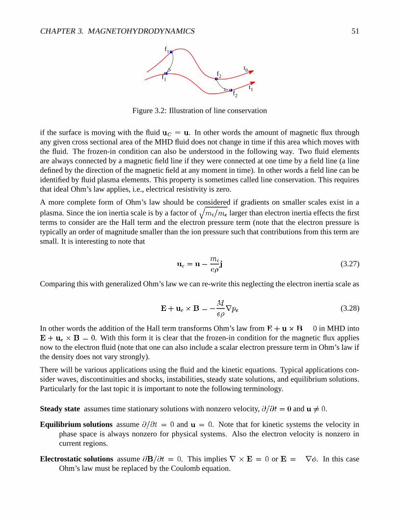
Figure 3.2: Illustration of line conservation

if the surface is moving with the fluid � � � � . In other words the amount of magnetic flux throughany given cross sectional area of the MHD fluid does not change in time if this area which moves withthe fluid. The frozen-in condition can also be understood in the following way. Two fluid elementsare always connected by a magnetic field line if they were connected at one time by a field line (a linedefined by the direction of the magnetic field at any moment in time). In other words a field line can beidentified by fluid plasma elements. This property is sometimes called line conservation. This requiresthat ideal Ohm’s law applies, i.e., electrical resistivity is zero.

A more complete form of Ohm’s law should be considered if gradients on smaller scales exist in aplasma. Since the ion inertia scale is by a factor of � � & 4 �

larger than electron inertia effects the firstterms to consider are the Hall term and the electron pressure term (note that the electron pressure istypically an order of magnitude smaller than the ion pressure such that contributions from this term aresmall. It is interesting to note that

� � � - � &� � > (3.27)

Comparing this with generalized Ohm’s law we can re-write this neglecting the electron inertia scale as� 4 � � � - � � � � A (3.28)

In other words the addition of the Hall term transforms Ohm’s law from� 4 � � � 2 in MHD into� 4 � � � 2 . With this form it is clear that the frozen-in condition for the magnetic flux applies

now to the electron fluid (note that one can also include a scalar electron pressure term in Ohm’s law ifthe density does not vary strongly).

There will be various applications using the fluid and the kinetic equations. Typical applications con-sider waves, discontinuities and shocks, instabilities, steady state solutions, and equilibrium solutions.Particularly for the last topic it is important to note the following terminology.

Steady state assumes time stationary solutions with nonzero velocity,� 4 � �,� 2 and �� 2 .

Equilibrium solutions assume� 4 � � � 2 and � � 2 . Note that for kinetic systems the velocity in

phase space is always nonzero for physical systems. Also the electron velocity is nonzero incurrent regions.

Electrostatic solutions assume� 4 � � � 2 . This implies

� � � � 2 or� � - ��

. In this caseOhm’s law must be replaced by the Coulomb equation.


3.4.2 Entropy and Adiabatic Convection

In an ordinary gas or fluid the change of heat due to pressure or temperature changes is

�#� � � ��E 4 A � �

Assuming an ideal gas (with 3 degrees of freedom)

E � A � 4 �and the specific heat and coefficients of specific heat

� � � � � � � � � ��

and the ratio � � � 4 � � � � 4��.

Thus the change in heat becomes

�#� � � � � � A 4 � � A � �� A �� AA 4 � ��

Entropy changes are defined as � �� 4 E

or

�� A � � �For adiabatic changes of the state of a system we have � �

� 2 which can also be expressed as

�� A � � � �� A�� 4 � �� A�� 2 (3.29)

with the specific volume �� & 4 � . This equation implies that the entropy of a plasma element does notchange (moving with this element). The same relation can be derived from the total pressure equation

& - &� �� A 4 �� A � � � - A ��

with the help of the continuity equation for density.

Exercise: Derive equation (3.29) from the pressure equation.


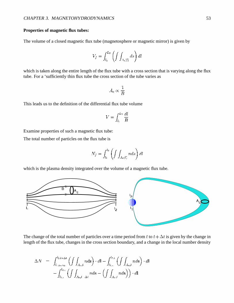
Properties of magnetic flux tubes:

The volume of a closed magnetic flux tube (magnetosphere or magnetic mirror) is given by

�� 2

��

which is taken along the entire length of the flux tube with a cross section that is varying along the fluxtube. For a ‘sufficiently thin flux tube the cross section of the tube varies as

5 � &�This leads us to the definition of the differential flux tube volume

� � � � ��

Examine properties of such a magnetic flux tube:

The total number of particles on the flux tube is

� � � � ��

' � 2�

��

which is the plasma density integrated over the volume of a magnetic flux tube.

� � �

� ��

� � �

The change of the total number of particles over a time period from�

to� 4 � �

is given by the change inlength of the flux tube, changes in the cross section boundary, and a change in the local number density

� � � � ��

� � � � � 7 � ' �� - � � ��

� � � � � 7 � ' �� 4 � � ��

� � � �� 7 �� ' � � - � � � �� 7 � ' ��


4 � � ��

� ' �#� 4 � ��)- ' �#��

��

� � � ��

� � � �� 7 � ' �� - � � � � ��

� � � �� 7 � ' �� 4 � � ��

� � � � 7 �� ' � � � � � � � � � � � 4 � � ��

� ' �#� 4 � ��+- ' ��

��

where 5 is the cross section of the flux, � � is the velocity of the boundary of the flux tube, and � � is

the line element along the flux tube boundary. The temporal change of the total number of particles inthe flux tube is

� � � � � � � � � � � � � ' �� 4 � � C � � � � � � ' ��4 � � ��

� � � 7 � ' � � � �� 4 � � �� 7 � ' �#� 4 � ��)- ' �#��

� � � ��

��

here � � C and � � � is the velocity of the flux tube boundary at the points� C and

� � . And in the limit� �� 2�

�� 7 � ' � � 4 � � C � � � � � � 7 � ' � �4 � � ��

�� 7 � ' � � � �� - � � �

�� 7 � �� ' � ��6�

F� � � � �� 5 � ��

� ' � � � - � ��

In other words the number of particle changes only as a result of a motion of the flux tube boundarydifferent from the plasma motion. In particular this implies that�

flow through the ends of the flux tube (into the ionosphere or out of a magnetic mirror configura-tion) can change the total number of particles on a flux tube�the number of particle does not change for closed ends (i.e., no flow through the ends) and idealMHD because the boundary of the flux tube are magnetic field lines and plasma elements movewith the magnetic field (= boundary of the flux tube).�using the definition of a differential flux tube

� � � ��' ��

is conserved in ideal MHD in the absence of flow at the ends of the flux tube


The above discussion considered the the total number of particles which is the integral over the numberdensity. For the derivation of the constancy of total number of particles on flux tubes we only requiredthat the number density satisfies a continuity equation. This implies that any property which satisfies acontinuity equation is conserved. In particular it can be shown that� A C�� 4 �� A C�� 2if heat flux and energy sources are negligible. For slow (adiabatic) changes the pressure is constant onmagnetic field lines such that we can define

� � A C�� A C�� Since A C�� satisfies a continuity equation the derivation for �

� 4��

follows exactly that for density suchthat �

� 4�� 2 for ideal MHD and no flux through the ends of a flux tube. Consider the specific

entropy of a flux tube as � � � �. This implies that the specific entropy satisfies

� �� A �

�� 2

This is a generalization of the local conservation of entropy

� A��

�� 2

The number of particle on flux tubes and the flux tube entropy are important to achieve insight into con-vection. Considering for instance the magnetosphere these quantities can be evaluated in the equatorialplane thus providing a two-dimensional map of flux tube entropy. Steady convection implies

� 4 � �%� 2 ,i.e., the magnetic and plasma configuration does not change. Thus steady convection can occur onlyalong contours of constant flux tube entropy.

Other equations of state:

The rigorous derivation of the MHD equations from the Boltzmann implies � � 4��. However there

are situations where it is more appropriate to assume other values for gamma to emulate a particularequation of state. We illustrate these using the equation for pressure.

& - &� �� A 4 �� A � � � - A ��

a) Adiabatic changes: The value of � � 4��corresponds to adiabatic change and we can transform the

pressure equation to an equation for adiabatic changes.

b) Isothermal changes: With A � '�� E we can re-write the pressure equation as


� E 4 � E 4 � �� E � - � - & � E �� Thus a value of � & leads to �

E 4��+� � E 4 � E 4 � �� E � 2 and implies isothermal changes.

c) Incompressible changes can be modeled in the limit of � 6 because this limit implies� � � � 2

such that � �4��+� 2 .

3.4.3 Conservation laws:

The MHD equation satisfy mass, momentum, and energy conservation.

� �� - �� 6�� 6�� - �� 6� � 4 � A 4 � �� & - &�� - �� &� � �*� 4 A - & 4 &� � � �� - � � �� 4 �� >�� with the total energy density

� � � � � &� � � � 4 A - & 4 &� �� (3.30)

Exercise: Demonstrate the validity of the energy conservation equation.

The various terms in (3.30) are the energy density of the

Bulk flow:C� � � �

3.5 MHD Equilibria

Resistive Diffusion

Before discussing equilibrium properties let us first consider effects of electric resistivity. Using theresistive form of Ohm’s law (with constant resistivity

�) and the induction equation

� � � � - � � ��

� � - �� 4 ��


In cases where the velocity is negligible one obtains� � � � �� This equation indicates that the magnetic field evolves in the presence of a finite resistivity even in theabsence of any plasma flow. This process is called resistive diffusion. Dimensional analysis yields forthe typical time scale

� �&� ��

�� i.e., diffusion is fast for large values of

�or small typical length scales. For the prior discussion of the

frozen-in condition we require that the resistivity is 0 or at least so small that the diffusion time is longcompared to the time scale for convection where the frozen-in condition is applied.

Basic equilibrium equations and properties:

Equilibrium requires� 4 � �%� 2 and � � 2 . Thus the MHD equations lead to

- � A 4 >�� 2� �� > (3.31)�� 2Taking the scalar product of the momentum equation with and > yields

�!� A � 2> �!� A � 2

In other words the pressure is constant on magnetic field lines and on current lines.

Note: There is no equation for the plasma density. Only the pressure needs to be determined. From

A � '�� Eit follows that only the product ' E is fixed and either density or temperature can be chosen arbitrarily.

The momentum equation can also be expressed as

�� A 4 � �� & - &�� 2


or

� � A 4 � �� - &� � �� 2This implies particularly simple equilibria for �.� � 2 (a simple case of this condition is a magneticfield with straight magnetic field lines). In this case the equilibrium requires total pressure balancewhere the sum of thermal and magnetic pressure are 0, i.e.,

� � A 4 � �� 2or

A 4 � �� (3.32)

A particular example of this class of equilibria is the plain current sheet with the specific example of aso-called Harris sheet with

� � � �� with

A � A �� > � � ��

with A �=� � �� 4 � � �� .

��

�

��

� ��

Note that one can add any constant to the pressure. It is also straightforward to modify the magneticfield, for instance to an asymmetric configuration. the pressure is computed from (3.32) and onlysubject to the condition that it must be larger than 0 everywhere.

The magnetic and plasma configuration also determines how important pressure relative to magneticforces are. It is common to use the so-called plasma � as a measure of the thermal pressure to magneticfield pressure (this is also a measure of the corresponding thermal and magnetic energy densities.). Theplasma � is defined as

� � � � � A� � 1


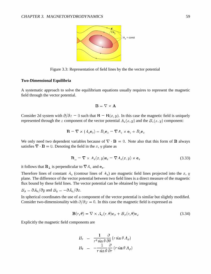
Az = const

Az

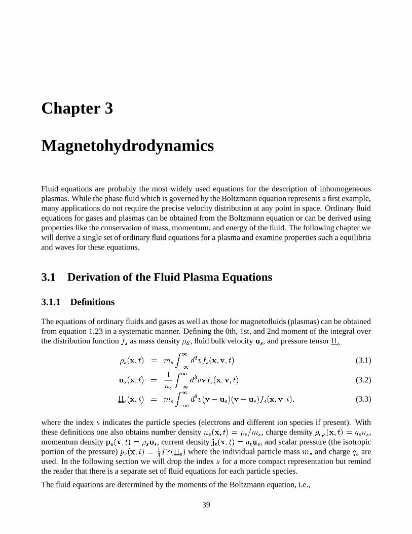
Figure 3.3: Representation of field lines by the the vector potential

Two-Dimensional Equilibria

A systematic approach to solve the equilibrium equations usually requires to represent the magneticfield through the vector potential. �� Consider 2d system with

� 4 � � � 2 such that � � � �� . In this case the magnetic field is uniquelyrepresented through the

�component of the vector potential

� � � �� and the� � � � �� component:

�%� � � �� 4 � �� 4 � ��We only need two dependent variables because of

� � � 2 . Note also that this form of alwayssatisfies

� � � 2 . Denoting the field in the � ,�

plane as

�� (3.33)

it follows that �� is perpendicular to� � and �� .

Therefore lines of constant � (contour lines of

� ) are magnetic field lines projected into the � ,�

plane. The difference of the vector potential between two field lines is a direct measure of the magneticflux bound by these field lines. The vector potential can be obtained by integrating� � � � � 4 � � and

� � - � � 4 � � .

In spherical coordinates the use of a component of the vector potential is similar but slightly modified.Consider two-dimensionality with

� 4 �� 2 . In this case the magnetic field is expressed as

� F �� %� � � � F �� 4 � � F �� (3.34)

Explicitly the magnetic field components are

��

� &F � �� F �� D� - &F �� F � F ��


Remembering that the gradient in theF,

plane is defined as

� �� F � � 4 &F � �� one can choose

�.� F �� such that � � � � 2 . It follows that magnetic field lines are determined

by

F �� ' 2 � (3.35)

Exercise: Consider the magnetic field� � � � �� 4

,� �

��

. Compute the equations for magneticfield lines.

Exercise: Repeat the above formulation for cylindrical coordinates with� 4 �� 2 .

With� � � � � � � � � �� )- � �� 4 � �� - � � �� the current density becomes

> � &�� 4 � � �� - &�� 4 &��

such that the�

component of the current density is

� � � - &� � � �

Substituting the current density in the force balance equation and using � � � � � �?� � � � � � -� � � � �

2 � - � A 4 > � � - � A 4 &�� - � � �� 4 � � � � �� 4 � �� - � A 4 &�� - � � � � - �� - � � � � �� - � A 4 &�� - � � � � - � � � � � 4 � � � � � ��

Here the term� � � � � � has only a

�component because

� � � and� � are both in the � ,

�plane.

Since it is the only term in the�

it follows that� � � � � � � 2 or

� � �� . Thus we can in generalexpress

� � �5� � � � � . This can be used to express


� � � � � � &� � � �� &� ��

� ��

In summary the force balance condition leads to� A � �� - &� ��

��

Since the pressure gradient is along the gradient of � the pressure must be a function of

� . It followsthat

� � � -�� A � � � 4 � � � � � ��

In this equation p represents the thermal pressure and� �� 4 � �� is the magnetic pressure due to the�

component of the magnetic field. In other words in two dimensions the magnetic field along theinvariant direction acts mostly as a pressure to maintain an equilibrium. Defining

�A � � �,� A 4 � �� we have to seek the solution to

� � � - � � ��

�A � � �"1 (3.36)

Usually�A � � � is defined as a relatively simple form. Most convenient for traditional solution methods is

to define�A � � � as a linear function of

� . More realistic is a definition which requires a kinetic back-ground. We will later show that local thermodynamic equilibrium implies A � � � � �� - � � 4 5 �where

5 is a constant which follows from the later kinetic treatment of the equilibrium.

Exercise: Consider A � � � � A � �� - � � 4 5 � and� � � 2 . Show that a one-dimensional (

� 4 � � � 2and

� 4 � � � 2 ) solution of equation (3.36) has the form � � 5 � � �� 4 ,�

and that themagnetic field in this case is the Harris sheet field.

Exercise: Consider one-dimensional solutions with� 4 � � �� 2 . Obtain the first integral of the equation

(3.36) by multiplying the equation with � � 4 � � and integration. The resulting equation is the

equation of total pressure balance. Interpret the term in the first integral in this manner.

Exercise: Consider a two-dimensional plasma� 4 � � � 2 with

� � � 2 and use the representation ofthe magnetic field through the vector potential. Replace the magnetic field in resistive Ohm’s law� 4 � ��

� � through the vector potential and show for� � ��

that this yields forthe z component

� � 4 � � 4 � � � � � �� . For

�0� 2 this equation directly demonstratesthe frozen-in condition. Explain why.

Note that the above discussion can be generalized to coordinate systems other than Cartesian. ForLaboratory plasmas with an azimuthal invariance it is often convenient to use cylindrical coordinateswith

� 4 � �.� 2 . If there is invariance along a cylinder axis one can also use� 4 � � � 2 .


▼α

▼β

α=const

β=const

B

Figure 3.4: Sketch of the field interpretation of Euler potentials.

Three-Dimensional Equilibria:

In three dimensions we cannot make the simplification of using a single component of the vector po-tential. However there is a formulation which lends itself to a similar treatment.

Introducing so-called Euler potentials � and � : � �� 4 �� =>

�� 4 ��

� � � � (3.37)

Note that Euler potentials imply � � � 2 which is not generally satisfied but it is always possible tofind a gauge such that is perpendicular to � .

Using Euler potentials the magnetic field is perpendicular to�� and

� � or - in other words - magneticfield lines are the lines where isosurfaces of � and � intersect. The prior two-dimensional treatment isactually a special case of Euler coordinates with �

� � and � � �.

The current density is now given by� � � � �� )- �� 4 � �� - � � �!� � > � &��

� � � � �� &�� - �

�� 4 � � ��@��

��)-1�

��,�@� � � ��

Force balance: � � � � � � � � � � � � - � � � � �

2 � - � A 4 > � � - � A 4 &��

� � � � �� - � A 4 &�� !� � ��

� � � � � � � �- � ��

� � � � � � � � �


This yields the basic dependencies of A � A �� and the equilibrium equations

� � �� A �

��

(3.38)��

� � � � �� -�� A �� (3.39)

Note that in cases with a gravitational force the force balance equation is modified to

- � A 4 > � - � �� 2where

�is the gravitational potential. This is for instance important for solar applications of the

equilibrium theory. In this case the pressure has to be also a function of � and the equilibrium equationsbecome

� � �!� � �� A �

��

��!� � ��

� � � � �� -�� A ��

� � - � A ��

These equation are often referred to as the Grad Shafranov equations and they are commonly used tocompute three-dimensional equilibrium configurations. While there are some analytic solutions theseequations are mostly used with computational techniques. A numerical procedure to find solutionusually starts with a straightforward initial solution. For instance, a vacuum magnetic field is alwaysa solution to equations (3.38) and (3.39) for constant pressure (vacuum field refers to a magnetic fieldfor which the current density is 0, i.e., there are no current carriers). Examples are constant magneticfields, dipole or higher multipole fields or any magnetic field which is derived through a scalar potential � - � � . Note that � has to satisfy

� � � 2 otherwise�� 2 is violated.

Magnetic dipole in spherical coordinates� F ��

:

� � - �� F � (3.40)

Noting that

� � � � �� F � � 4 &F � �� 4 &F �� the dipole magnetic field components become


��

� - �� F��D� - ��

�� F�

The formalism derived for spherical coordinates in two dimensions can then be used to derive Eulerpotentials for the start solution. In the course of the numerical solution of (3.38) and (3.39) the pressureis increased as a specified function of � and � . Also any changes in terms of boundary conditions etc.are applied in the iterative solution of the equations. Note that a nontrivial point of the system (3.38)and (3.39) is the existence of solution or possible multiple branches of solutions for the same boundaryconditions.

Exercise: Determine the vector potential component

� for the dipole field and derive the equationsfor the magnetic field lines in spherical coordinates.

3.6 MHD Stability

The stability of plasmas both in laboratory and in the natural environment is of central importance tounderstand plasma systems. It is worth noting, however that the interest of laboratory plasma researchis usually the stability of a configuration (for instance the stable confinement of plasma in a fusiondevice) while the interest in space plasma is clearly more in the instability of such systems. Either wayplasma instability is a central issue in both communities.

A priory it is clear that a homogeneous plasma with all particle species moving a the same bulk velocityand all species having equal temperatures with Maxwell particle distributions is the ultimate stablesystem because it is in global thermal equilibrium. However, any deviation from this state has thepotential to cause an instability. In this section we are interested in the stability of fluid plasma such thatdetail of the distribution function such as non-Maxwellian anisotropic distributions cannot be addressedhere and will be left for later discussion.

In the case of fluid plasma the main driver for instability is spatial inhomogeneity, such as spatiallyvary magnetic field, current, and bulk velocity distributions. Most of the following discussion willassume that the bulk velocity is actually zero and the plasma is in an equilibrium state as discussed inthe previous section.

There are several methods to address plasma stability/instability. First, modern numerical methodsallow to carry out computer simulation if necessary on massive scales. Numerical studies have advan-tages and disadvantages. For instance, a computer simulation can study not only small perturbationsbut also nonlinear perturbations of the equilibrium and the basic formulation is rather straightforward.However, a simulation can test only one configuration, one set of boundary conditions, and one typeof perturbation at a time. thus it may be cumbersome to obtain a good physical understanding of howstability properties change when system parameter change.

There are two basic analytic methods to study stability and instability of a plasma. The first methodsuses a small perturbation and computes the characteristic evolution of the system. If all modes are have


constant or damped amplitudes in time the plasma system is stable, if there are (exponentially) growingmodes the system is unstable. This analysis is called the normal mode analysis. The second approachalso uses small perturbations but considers a variational or energy principle. This is similar to a simplemechanical system where the potential has a local maximum or minimum. Thus this method attemptsto formulate a potential for the plasma system which can be examined for stability. It will soon be clearthat although the basic idea is the same, plasma systems are considerably more complex than simplemechanical examples.

3.6.1 Small oscillations near an equilibrium

Consider a configuration which satisfies the equilibrium force balance condition. For conditions- � A 4> � � 2 . Equilibrium quantities are denoted by an index 0, i.e., A � , � , and > � � C

� � � � . All

equilibrium plasma properties are a function of space only.

In the following we assume small perturbations from the equilibrium state. For these perturbations weuse the index 1. The coordinate of a fluid element is

� �#��. Considering a small displacement of the

plasma coordinate in the frame moving with the plasma (Lagrangian displacement) such that the newcoordinate is

,�#�� #�� 4�� # �/��which satisfies � �� 2 � � 2 . A Taylor expansion of the fluid velocity yields

� C �#+�� C �# � �� 4 � �� C �# �� 4 1 1 1with

�� 4 � � . However, since both � and � C are perturbation quantities (and hence small) we can

neglect the terms of the Taylor expansion except for the 0th order implying:

� C �# �� C �� Here � C ��

represent the Eulerian velocity at the location

and � C �# � �� the Lagrangian descriptionin the co-moving frame. Since � C �#�� # �/��4 � � . Therefore we can replace replace the Eulerianvelocity in the plasma equations by the Lagrangian by

� � �# � ��4 � � .We now linearize the ideal MHD equations around the equilibrium state and substitute � C with

� � 4 � � .� � C� � � - � � � � � ��

� � � � �� - � A C 4 &�� C � � � 4 &�� C� C� � � � � � �� A C� � � - �� A �%- A � ��


We can now integrate the continuity equation, the induction equation, and the pressure equation in time(assuming that the initial perturbation is zero) which yields

� C � - � �6� � � � � C � � � � � ��

A C � - � �� A �%- A � �� and substitute � C with

�� . Take the time derivative of the momentum equation and replace the perturbed

density, magnetic field, and pressure in the momentum equation.

� � � � �� @� � �� A � 4 A � �� 4 &�� 4 � � ��

To solve this equation it is necessary to provide initial conditions for � � �� C , and boundaryconditions for � .

Boundary Conditions

Frequently used conditions for a laboratory systemare that the plasma is confined to a region whichis embedded in a vacuum which in turn is boundedby an ideal conducting wall. This is an assumptionseldom realized but suitable for the mathematicaltreatment.

�

�

� ��

��

In the case of space plasma systems boundary conditions are even more difficult to formulate becausethey are not confined to a particular region. However, if the volume is taken sufficiently large surfacecontributions to the interior are small such that for instance an assumption that the perturbations arezero at the boundary is a suitable choice. In the case of solar prominences the field is anchored in thesolar photosphere which is an almost ideal conductor which implies that the foot points of prominencesare moving with the photospheric gas.

i) Conducting wall

If the boundary to the plasma system is an ideal conducting wall the boundary condition simplifiesconsiderably. In this case it is necessary that the tangential electric field is zero because the wall has aconstant potential:

�� C � 2where �� is the unit vector of the outward normal direction to the wall. With Ohm’s law

� C � ��

we obtain�� ;� �� - � �� =� 2


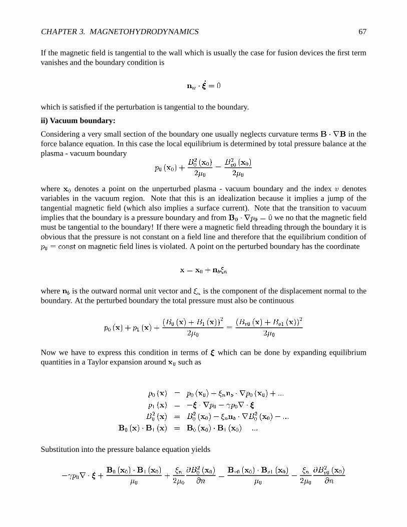
If the magnetic field is tangential to the wall which is usually the case for fusion devices the first termvanishes and the boundary condition is

�� 2which is satisfied if the perturbation is tangential to the boundary.

ii) Vacuum boundary:

Considering a very small section of the boundary one usually neglects curvature terms � � in theforce balance equation. In this case the local equilibrium is determined by total pressure balance at theplasma - vacuum boundary

A � �� "� 4 � �� + � �# �"�� where

�denotes a point on the unperturbed plasma - vacuum boundary and the index � denotes

variables in the vacuum region. Note that this is an idealization because it implies a jump of thetangential magnetic field (which also implies a surface current). Note that the transition to vacuumimplies that the boundary is a pressure boundary and from � �� A � � 2 we no that the magnetic fieldmust be tangential to the boundary! If there were a magnetic field threading through the boundary it isobvious that the pressure is not constant on a field line and therefore that the equilibrium condition ofA �?� ��

on magnetic field lines is violated. A point on the perturbed boundary has the coordinate

� �� 4 � � ��

where � � is the outward normal unit vector and �� is the component of the displacement normal to theboundary. At the perturbed boundary the total pressure must also be continuous

A � �# � 4 A C �# � 4 �� # � 4 � C �# �� + �+�� 4 � + C �# �� Now we have to express this condition in terms of � which can be done by expanding equilibriumquantities in a Taylor expansion around

�such as

A � �# � � A � �# � � 4 �� !� A � �# �"� 4 1 1 1A C �# � � - � �� A �,- A � � � �� # � � � �� # � � 4 �� 4 1 1 1 � �# � � C �# � � � �# �"� � C � �"� 4 1 1 1

Substitution into the pressure balance equation yields

- A � �� 4 � �# �"� � C �� "�� 4 �� ' � + �)�# � � � + C �#�� 4 �� + � �#�� '


where we have made use of �� being along� A � .

A second boundary condition can be obtained from the fact that the electric field in a frame movingwith the plasma velocity is zero

� C 4 � C � � � 2 and the tangential component must be continuousinto the vacuum region, i.e.

� � � �� + C 4 � C �� + �"� � 2This condition can be expressed as

� � � � + C � � � � � � C � + �=�5�� + �

Introducing the vector potential for the perturbation in the vacuum region � the electric and magneticfields are

� + C � - � �� C �%� � �which yields

� � �� - �� + �on the conducting wall the boundary condition for � is

�� 2i.e., the vector potential has only a component along the normal direction of the wall

3.6.2 Energy principle

We have derived an partial differential equation of the form

� � � � �� -�� where

�is the differential operator

� � � � - �@� � �� A � 4 A � �� )- &�� 4 �� %� � � � � � �

Assuming


� �� the PDE becomes an Eigenvalue equation for � � :

� � � � � � � � �and stability depends on the sign of � � . In the MHD case the operator

�is self-adjoint, i.e.,

� � � � � � � � 0� � � � � � � � � where the integrals are carried out over the plasma volume. The eigenvalues of a self-adjoint operatorare always real that means either positive or negative. Explicitly the Eigenvalues are given by

� �%� � � � � � � � � � � � � � � � � For � �� 2 the values for � are real and the solution is oscillating but not growing in time, i.e., thesolution is stable. However if there are negative eigenvalues � �� 2 there are solutions which aregrowing exponentially in time and are therefore unstable!

In the following it is demonstrated that�

is self-adjoint:

� � � � � � � � � � � � � -�� @� � �!� A � 4 A � � � � � � - &�� 4 � � �� Identities to be used:

�� !� � 4 � �� )- � �6� � �� 4 �� 4 �� %� � � � � � �

which yields

� � � � � � �� A � 4 A � ��


4 &�� - &��

-�� !� A � 4 A � � � � �)- &�� "� � ��

� � � � A � � � � �� 4 &��

4 � � � � �� A � � � � - &��

-�� A � 4 A � �� - &��

� � 2where we have used Gauss theorem for the surface integrals with

��

� 2 on the plasma boundary.

With the boundary conditions derived in the prior section

- A � �� 4 � �� "� � C �# �"�� 4 �� # �"�� ' � + � �# �"� � + C �#��"�� 4 �� + � �� ' � � &�� C � � � � �

For the surface terms we can use the boundary conditions

�� 7 � � � -�� A � 4 A � �� - &�� 2� - � � �� A � 4 � � �� - + � � � + �� 4 �� +- � �+ � �# �"�� ' � �

� � 2- � � �� - &��

� � 2� - � � �� A �� ' - + � � � + �� 4 �� )- � �+ � �# � �� ' � �

� � 2and the field terms in the vacuum region can be treated as follows

�� 7 � � � � �� + � � �� 2

� � �� 2� � ��

��

��

��

��

��


such that the sum of the surface terms can be written as

� � 7 � � � - � � �� A �� ' 4 &� �� #��"�)- � �+ � �� "�� ' � �� 2 4 &��

��

��

Here it is clear that the surface contributions are symmetric in � and�.

Finally we have to demonstrate the symmetry of the remaining non-symmetric terms

�� A � �� - &��

Consider decomposition of

� � � � 4 � � � � � � ��

� � � � 4 � � � � � � � � �Considering that � � �� A � �

� � �� A � � 2 and�� 2 the non-symmetric parts

of the integral reduce to

�� A � �� - &�� The contributions from � � � � � can also be symmetrized. The algebra is somewhat more tedious andwe note that the integrand for the � � may be reduced to a form

� � � � �!� A � � � . This give a contributionof � � 7 � � � � � � � � � �

�

� 2 but for typical boundary conditions it is assumed that the normal magneticfield is 0 (i.e. the magnetic field is aligned with the boundary).

To show the symmetry of the perpendicular components it is necessary to decompose the perpendic-ular displacement into components along the equilibrium current and along the equilibrium pressuregradient:

� � � � C �� > � 4 � � �� C �� > � 4 � � �� A �� A � �

With these definitions consider the term

- � � � � > � � � � � � � - � � � � � > � � � � � �� C �� > � 4 � � � � �� - � � � � � > � � � � � � � C �� A � 4 � � � �� - � � � � � > � � � �� C � � A � 4 � C �� A � � �- � � � � � > � � � � � � � � � � � � 4 � � � � � � ��


� -�� > � �� A � � � � C - � > � �� C � � A � �- � � � � � > � �� - � > � �� 4 � � > � � � � � � � � � �� A �"� � > � �� C �� A � � � � �� )- � � � � � � > � � � � � � �� A � �� - � � � � � � > � � � � � � �� Thus the sum of the non-symmetric integrands becomes

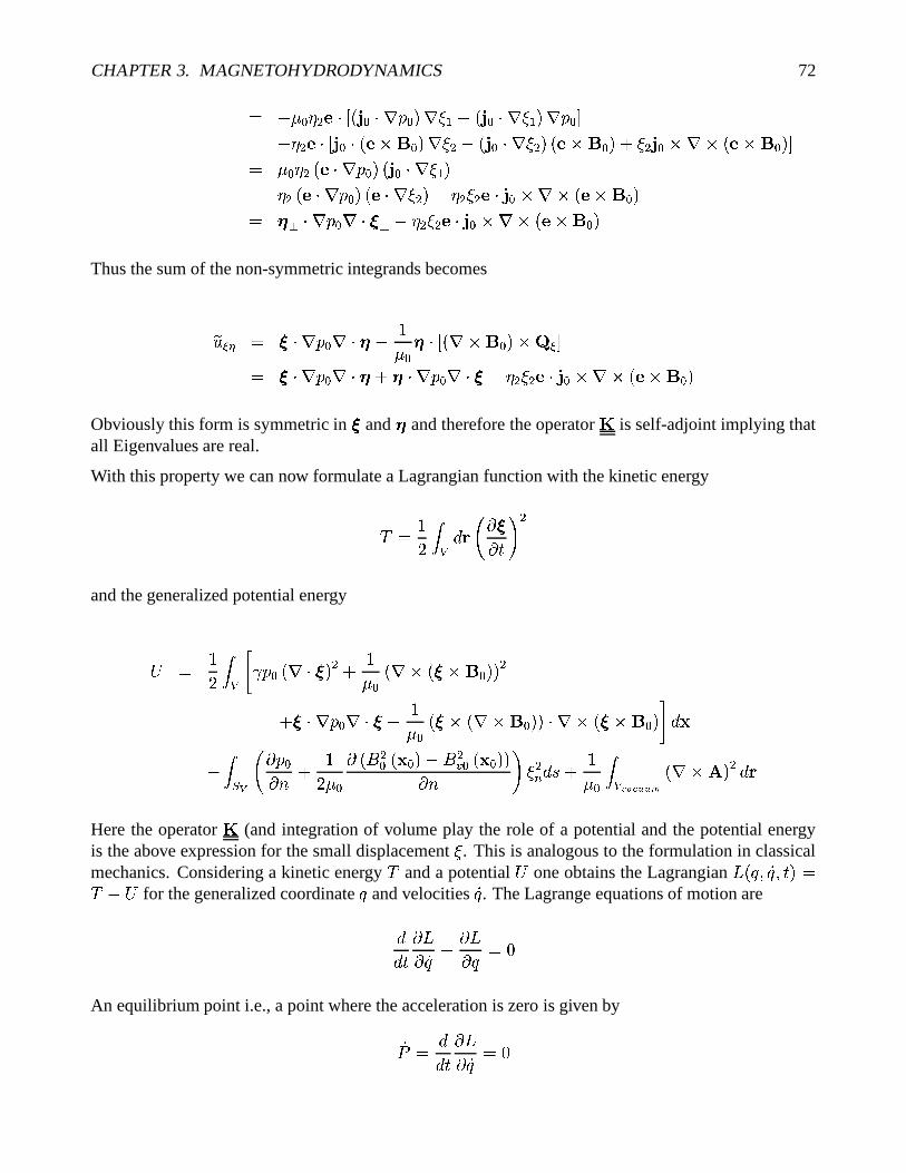
�� A � �� - &�� A � �� 4 � �� A � �� - � � � � � � > � � � � � � � � �Obviously this form is symmetric in � and � and therefore the operator

�is self-adjoint implying that

all Eigenvalues are real.

With this property we can now formulate a Lagrangian function with the kinetic energy

E � &� � � � � � ��

and the generalized potential energy

� � &� � � � A � � �� 4 &�� 4 � �� A � �� - &�� "� � �

- � � �

� � A �� ' 4 &� �� #�� )- � �+ � �� ' � � �� 2 4 &��

��

Here the operator�

(and integration of volume play the role of a potential and the potential energyis the above expression for the small displacement � . This is analogous to the formulation in classicalmechanics. Considering a kinetic energy

Eand a potential

�one obtains the Lagrangian

3�#: ��: �� E - �for the generalized coordinate

:and velocities

�:. The Lagrange equations of motion are

�� : - � � : � 2

An equilibrium point i.e., a point where the acceleration is zero is given by

�� : � 2


which implies � � : � - � �� : �� / � � 2We now define the coordinates as � � : - : �

and assume the � to be small displacements from theequilibrium point. The potential can be expanded in terms of the displacement at the equilibrium pointi.e.

� � � � � � �#: �"� 4 � � �#: �"�� : � 4 &� � � � � : �"�� : � � � 4 1 1

Substituting � and in the Lagrangian with the kinetic energy� � �� yields the equation of motion

�� 4 � � � �#: �"�� : � � � 2with the solutions

� � �� &� � � � � : �"�� : � � � F � � � � : �"�� : � � 2� � � �� ?� - &� � � � � : �"�� : � � � F � � � � : �"�� : � � 2

Thus the solution is oscillatory and therefore stableif the potential has a local minimum and the solu-tion is exponentially growing if the potential has alocal maximum. ��

ξ �

ξξ1

Stability: d2V/dξ2>0 ��

ξ �

ξξ1

Instability: d2V/dξ2<0

��ξ�

ξ

��

Equilibrium: dV/dξ=0

ξ1 ξ3ξ2

The energy principle for the MHD equations has to be interpreted in a similar way. An equilibriumis stable if the potential energy is positive for all small perturbations � and it is unstable if there areperturbations for which the potential energy can become negative (Note that the equilibrium value ofthe potential is 0.


3.6.3 Applications of the energy principle

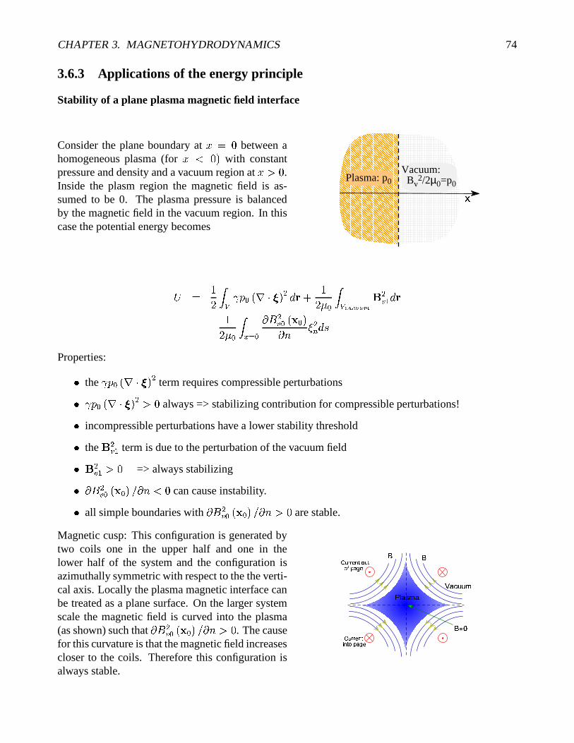
Stability of a plane plasma magnetic field interface

Consider the plane boundary at � � 2 between ahomogeneous plasma (for � � 2 � with constantpressure and density and a vacuum region at � � 2 .Inside the plasm region the magnetic field is as-sumed to be 0. The plasma pressure is balancedby the magnetic field in the vacuum region. In thiscase the potential energy becomes

�

Plasma: p0Vacuum: Bv

2/2µ0=p0

� � &� � � A � � �� 4 &� �� + C � 4 &� �� / �

� � �+ � �#��"�� ' � �� 2Properties:�

the A � �� term requires compressible perturbations� A � � �� 2 always => stabilizing contribution for compressible perturbations!�incompressible perturbations have a lower stability threshold�the �+ C term is due to the perturbation of the vacuum field� �+ C � 2 => always stabilizing� � � �+ � �� 4 � ' � 2 can cause instability.�all simple boundaries with

� � �+ � �# � ��4 � ' � 2 are stable.

Magnetic cusp: This configuration is generated bytwo coils one in the upper half and one in thelower half of the system and the configuration isazimuthally symmetric with respect to the the verti-cal axis. Locally the plasma magnetic interface canbe treated as a plane surface. On the larger systemscale the magnetic field is curved into the plasma(as shown) such that

� � �+ � �# � ��4 � ' � 2 . The causefor this curvature is that the magnetic field increasescloser to the coils. Therefore this configuration isalways stable.

��

� � ��

� ��

�� "!$#$%��

�� & �� '!$#$%��


A similar result is obtained for the interchange instability. This is an instability where a flux tube fromthe plasma region is bulging out into the vacuum region and vice versa vacuum flux tube enters theplasma region. This instability also requires a magnetic field line curvature opposite to that shown forthe cusp configuration.

The plasma can be unstable if� � �+ � �# � ��4 � ' � 2 . Consider the same simple plane plasma vacuum

boundary as before with � �� , and + �?�%� + � �� .

Consider a test function for the displacement and the vacuum perturbation field of the form

� � �

� � �� 4 � � 4 � � � � � �� 4 � � 4 � � ��where we dropped the indices � because we discuss exclusively the perturbed field in the vacuumregion. The normal component of the perturbation field is given by� C � � � � � � �� + �The perturbed field in the vacuum region satisfies

� � � �� C � � � � �� C � 2�� C � �� C � 2which yields

� �?� 2or � � � � � � � 4 � �� . Since the current density in the vacuum region is zero we can use

� C � � �� C � - � � � C � � 2or� C � �;� � � 4 � � � C in

�� C � 2 to obtain the y and�

components of the perturbed field� C � - � � � � � 4 � �� C �� C � � - � � � � � 4 � �� C �Thus we obtain � C � � � � C � � � 4 � � C � � 4 � � C � � � �

� � & 4 � � �� 4 � �� C � � � � � � � C � � � � � � � �� - � � � � 4 � ��


Since the Magnetic field is exponetially decreasing the perturbation � � has to take the also form

� � � �

� � � �� - � � � 4 � �� 4 � � � �such that

� C � � � �� + � � �� - � � � � 4 � �� and integration over the entire vacuum region from � � 2 to 6 yields

� �� + C � � � � / � �

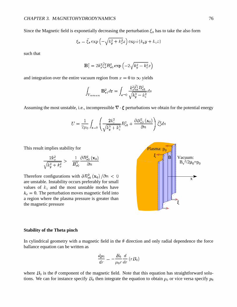
�� + �� 4 � �� 2Assuming the most unstable, i.e., incompressible

�%� � perturbations we obtain for the potential energy

� � &� �� / �� 4 � �� + � 4

� � �+ � �� ' ��

� �� 2This result implies stability for� � ��

� � � 4 � �� - &� �+ �� + � �� "�� '

Therefore configurations with� � �+ � �� "� 4 � ' � 2

are unstable. Instability occurs preferably for smallvalues of � � and the most unstable modes have� � � 2 . The perturbation moves magnetic field intoa region where the plasma pressure is greater thanthe magnetic pressure

Plasma: p0

Vacuum: Bv

2/2µ0=p0

x

ξ

ξ

Β

Stability of the Theta pinch

In cylindrical geometry with a magnetic field in the

direction and only radial dependence the forceballance equation can be written as

� A�

�F � - � �� F ��

F � F � � �where

� �is the

component of the magnetic field. Note that this equation has straightforward solu-

tions. We can for instance specify� �

then integrate the equation to obtain A � or vice versa specify A �


to integrate and obtain� �

. This is similar to the case of straight field lines in cartesian coordinates,however, for the

pinch field lines are curved and � � �� 2 . A straightfarward solution for this case

can be found by assuming the current density (along�) to be constant up to a radius

for which the

pressure drops to 0. forF �

the current density has to be 0 otherwise the pressure would be reuirednegative which is unphysical.

Exercise: Assume a constant current� �

along the�

direction in a cylindrical coordinate system. Com-pute the magnetic field

�� F �and integrate the force balance equation to obtain A � F �

. The pres-sure at

F � 2 is A � . Determine the critical radius for which the pressure decreases to 0.

The resulting configuration is a column or cylinder in wich the current is flowing along the cylinder axisin the

�direction and the magnetic field is in the azimuthal

direction. An equilibrium configuration

which has somesimilarity with the

pinch is the � pinch in which the magnetic field is along the zdirection and the perturbations of this configuration have the form

� � F �� F � �� where m is the wave number in the

direction.

In cylindrical coordinates the perturbations contributing to the potential energy are

�� &F �� F � F � � � 4 &F � � �� 4 � � �� "� � - � � � &F � � �� - � &� � �� F �� 4 � � �� 4 &F � � �� "� � &F �� F � F � � � � � � � � - � � � � �

We will assume that the boundary is a conducting wall at which the displacement is 0. With theserelations the potential becomes

� � &� � � � A �)�� 4 � A� F � � �� 4 � �� &� � �� F � � � � � � 4 � � �� 4 &F � � � � �� 4 &F � � � � ��

4 � �� F �� F � F � � � � � �F � � �� 4 � � � &� � �� F � � � � � � 4 � � ��


Azimuthally symmetric perturbations

In this case�

is zero and all

derivatives are 0. To evaluate the stability we bring the potential into thequadratic form

� � &� � � � C C � �� 4 � C � � �F � � � 4 �.� � ��F � � �

where the coefficients are

C C � � 4 � � � � �� A �� C � � �� =F 4 � � �

� � A �� =F - & �.� � �

�� =F - & � C �

and stability requires C C �.� - � C � � 2Using the force balance equation one can simplify the stability equation to

- �� A �

�� F � - F

A � � A�

�F � � � 4 �

For the

pinch the plasma pressure decreases with radial distance from the pinch axis such that at largedistances �� & . Here the rhs assumes a maximum such that stability requires

� AA � - � � FFor

A � � F � � �However to avoid plasma contact with the wall the density and pressure must be close to 0. Thus the

pinch is unstable with respect to symmetric perturbations which lead to a periodic pinching of theplasma column.


Azimuthally asymmetric perturbations

In this case the

dependence is nonzero and on can assume a displacement of the following form

� � � � � � F � �� F � �� F � ��

To simplify the analysis one usually assumes� � � � 2 . With this assumption the only change in the

potential energy is that the term A � �� is replaced by� �� F � � � �� 4 � �� Stability is obtained for

- �� A �

��?F � - F

A � � A�

�F � � �

�One can compare the stability limit for non-symmetric perturbation with that for symmetric perturba-tions. For small values of � the symmetric condition is always more unstable. For values with � � &the

� � & or even� � �

mode can be unstable even though the symmetric condition may implystability.

The� � & mode is called kink instability (or corkscrew instability because of the form of the bending

of the plasma collumn.

Stability and magnetic flux tube volume

In a plasma with a small plasma � the evolution is strongly dominated by the magnetic field such thatmagnetic flux tubes carry much of the energy. we had defined the magnetic flux tube volume as

� � � ��

The thermal energy contained in a flux tube is A � and since the flux tube volume changes duringconvection the energy associated with the flux tube changes. Using the pressure equation we have

A 4 � A � A - A �� A 4 A � ��Note that � A

4�� - A � � � and

�� - C� � �� - C� � �� which is obtained from

� �� A �

�� 2


The pressure change in the vicinity of the flux tube is

A � � 4 � � � � A 4 � A� ��

Considering a small displacement from the equilibrium: If the pressure change in the flux tube is greaterthan the pressure in the surrounding tubes then lower energy state is the equilibrium and energy has tobe brought into the system to achieve the change. In other words the configuration is stable for A � �� 4 � A� �

� � � 2or

- � A � A� ��

or - �� A

��

Note that adiabatic convection yields

- �� A

��

� For the sheet pinch this yields

- �� A

�� F � �

which is the small � approximation of our prior result.

Note, however that this is somewhat heuristic or intuitive and lacks the rigour or the prior discussion.

3.7 Magnetohydrodynamic Waves

In the following we want to examine typical waves in the single fluid plasma. The treatment is similarto for instance sound waves but clearly one expects that the magnetofluid has more degrees of freedomand wave propagation should depend on teh orientation of the magnetic field, i.e. it is not isotropic as inthe case of sound waves. Note that in the cause of waves in gravitationally stratified atmosphere wavepropagation is also nonistropic and gravity allows for a new wave mode the so-called gravity wave.

In the case of MHD we start from the full set of linearized ideal MHD equations.


� �� - � � �6�� 6�� - � �6� �6� � �)-1� A 4 &�� A� � � - � �� A - A � � �where we have already combined the induction equation and Ohm’s law. Now we linearize the equationas in the previous section, however, we do not introduce a small displace but rather keep � C as a variable.Specifically the MHD variables are expressed as

� � � � 4 � C� � � C � � 4 CA � A � 4 A C

For simplicity we assume all equilibrium quantities to be constant, i.e., we do not consider and inhomo-geneous plasma. Substitution of the perturbations into the MHD equations yields similar to the smalldisplacement treatment

� � C� � � - � � �� C� � � � C� � � - � A C 4 &�� C � � �� C� � � � � � � C �� A C� � � - A � �� C

Taking the second derivative in time of the momentum equation yields

� � � � � C� � � � - � � A C� � 4 &�� C� � � � �� A � �@� �� C � 4 � �� C � � � ��

where we used �=�5� � � � . Now dividing by � � and with the definitions for the speed of sound � � andthe Alfven speed �

�


� � � � A ��

we obtain � � � C� � � � � � � �@�� C � 4 �� C � � � ��

We will now try to find the solution as plane waves by assuming

� C � �� C � �� - � � ��which leads us to

� � � C � � � � � � � � � C �)-�� C � � � � ��

We now choose a coordinate system where the�

axis points along the equilibrium (constant) magneticfield and the

�vector is in the � ,

�plane and given by

� � � � � � 4 � � ��This leads to the following three components for the equation:

� � � - �� - � � � � 4 �

�� C � - � � � � � � � � C � � 2� � � - �� C � 2� � � - � � � � � � � � C � - � � � � � � � � C � � 2

or in matrix form � � � C � 2�� - �

�� - � � � � 4 �� 2 - � � � � � � �2 � � - �

�� 2- � � � � � � � 2 � � - � � � � � ��

�� C �� C � C �� 2

Exercise: Derive the above matrix.


These equations are linear independent and provide nontrivial solutions if the determinant is equal tozero.

a) Alfvén wave:

The first nontrivial solution is determined by the�

component of the above equations. This compo-nent separates from the other two because

� C does not appear in the first and third equation. In thedeterminant � � - �

�� appears a a common factor. The solution is

� �?��

or

� � � � � �� "� C�� The group velocity

$��

4�

�is

$�� "� C��

which is independent of�

and always along the magnetic field. The phase velocity is

� ��

where theta is the angle between�

and � . This wave is the Alf\ven wave.

A common representation of phase and groupvelocities is the Clemmov-Mullaly-Allis diagramwhich represents phase and group velocities in a po-lar plot where the radius vector represents the mag-nitude of the velocity and the angle is the propaga-tion angle theta. Note that the direction of the groupvelocity for Alfv\’en waves (which is the directionin which energy and momentum is carried) is al-ways along the magnetic field! Note also that thecase for

0�� 2�� is singular in that wave does notpropagate and the points with

�� 2 � should beexcluded from the group velocity plot.

��

θ

ω/ �

� �

Further properties of Alfvén waves:

� Velocity perturbation �� Wave is incompressible: �� "!$#&%'� �(��!*) or �(��%

CHAPTER 3. MAGNETOHYDRODYNAMICS 84�Magnetic field perturbation: C � - � � � � C �� =� - � � � C , i.e., the magnetic field perturba-tion is aligned with the velocity perturbation (and both are perpendicular to

�and � .�

Current density > C � � � � , i.e., the current perturbation is perpendicular to�

and � .�Alfvén wave also exist without steepening with nonlinear amplitudes.

Considering a localized perturbation for C along the�

vector propagation of an Alfven wave and thedeformation of the magnetic field is presented in the following figure.

��

��

�

� �

�

�

�

�� !� �#"%$ �'&(� ��

)

*

+ ,- ,

� .

The Alfvén wave is of large importance in many plasma systems. It is very effective in carryingenergy and momentum along the magnetic field. Among many space plasma applications the Alfvénwave is particulalry important for the coupling between the magnetosphere and the ionosphere. Hereperturbations (convection) from the magnetosphere are carried into the ionosphere and depending onionospheric conditions cause convection in the high latitude ionosphere.

A coomon diagnostic to identify Alfvén waves in space physics is the use of the so-called the Walenrelation.

� � � � � $ �.� � � � �� This relation is valid for linear and nonlinear Alfvén waves, and can also be used to identify the corre-sponding (nonlinear) discontinuities.

b) Fast and slow mode:

The other nontrivial solution is given by� � � � � 2 or

� � � -�� - � � � � 4 �

�� - � � � � � � � - � / � � � � � �� 2This is the dispersion relation for 4 additional solutions which are given by the roots of the equation.Since the equation is double quadratic, i.e., depends only on � � there are two different solutions for � � .Abbreviating � � � � � � � 4 �

��(where the

�stands for fast mode - the reason for this will be clear in a

moment) one can re-write the equation as

� / - � � � � � � � 4 �� =� 2 (3.41)


with the solutions

� �D� � ��

� / � - �� C��

� � �� 3�� 4 � � � � ( � � �� 4 � � � � � - � � �� ,) C��

Here the solution with the 4 sign is called the fast mode and the solution with the-

sign the slowmode.

Fast wave:

This is the MHD wave with the fastest propagation speed, i.e., information in an MHD plasma cannottravel faster thant this velocity.�

Phase speed along the magnetic field: � � 4 � � � � � ��

Phase speed perpendicular to the magnetic field � � 4 � � � � � � � �� 4 � � ��

Limit for � � � � ��

: � � -�� 2 => the fast mode becomes the so-called compressional

Afvén wave. Note that the compressional Alfven waves has a group velocity equal to its phasevelocity (different from the regular or shear Alfven wave).�Limit for �

�� : � � - � � � � � � 2 => the fast mode becomes a sound wave.

The most prominant example of a fast wave in space physics is the Earth’s bow shock. This shockforms as a result of the solar wind velocity which is faster than the fast mode speed. The fast waveis also important in terms of transporting energy perpendicular to the magnetic field. The slow modegroup velocity is as for the Alfven wave along the magnetic feild and it is comparably small. Thus thefast wave is the only MHD wave able to carry energy perpendicular to the magnetic field.

� ��

� �� ! "# $ �&% ��! " '�(

) *+ , -�. /0 1

0 2 3 4/�5 6�78 6�9 :

; < />=8 6�9 :?�@ 6BA�CD : 5 6 0FE = E :F/

Slow wave:


The slow wave is the third of the basic MHD waves. The phase velocity is always smaller than or equalto

� �� . Basic properties:

Phase speed along the magnetic field: � � 4 � � � �� .

Phase speed perpendicular to the magnetic field � � 4 � � � 2 .In the limits of � � � � �

��and �

�� the slow wave disappears.

Applications of the slow wave are not as eye catching than those for the other MHD wave but the waveis important to explain plasma structure in the region between the bow shock and the magnetosphere,and well know for applications such as magnetic reconnection.

Concluding remarks:

There is an additional wave which in MHD which is the sound wave. This is obtained by using� � � 2

and � � � 2 such that the velocity perturbation is along the magnetic field and thus the magnetic fieldperturbation is 0. However, it is singular in that it exists only for propagation exactly along the magneticfield, i.e. the velocity is exactly parallel to � and the

�vector is also exactly parallel to � . In fact the

sound wave can be either part of the slow wave or part of the fast wave solution depending on whether� � � � �

��or � � � � �

��.

Exercise: Derive the dispersion relations for�

parallel to � . What are the three wave solutions.

It should also be remarked that similar to a sonic shock wave the MHD waves are associated withrespective shocks or discontinuities, I.e., there is a fast shock for the transition from plasma flow that issuper-fast (faster than the fast mode speed) to sub-fast (slower than the fast mode speed), a slow shock,and an intermediate shock corresponding the Alfvén wave.

Documents

Chapter 3 Magnetohydrodynamicshow.gi.alaska.edu/ao/plasma/script/chap3.pdfChapter 3 Magnetohydrodynamics Fluid equations are probably the most widely used equations for the description